Estimation of Buildings’ Energy Efficiency via a Surrogate Regression Model

Luis G. R. Santos; Ido Nevat; Jordan Ivanchev; Mathias Niffeler

doi:10.20944/preprints202401.2062.v1

Preprint

Article

Estimation of Buildings’ Energy Efficiency via a Surrogate Regression Model

This version is not peer-reviewed.

Luis G. R. Santos^*,

Ido Nevat,Jordan Ivanchev,

Mathias Niffeler^*

Luis G. R. Santos^*,

Ido Nevat,Jordan Ivanchev,

Mathias Niffeler^*

This version is not peer-reviewed.

Downloads

114

Views

Comments

Submitted:

29 January 2024

Posted:

30 January 2024

You are already at the latest version

Abstract

Building energy demand impacts a myriad of interconnected economic, societal, and environmental aspects. As a result, Buildings Energy Models (BEM) play an important role in the process of urban design and planning. While previous studies have investigated the effects of building interventions on energy efficiency, their applicability may be limited due to the BEM’s high computational complexity. This limits their ability to systematically study important aspects of energy demand on a large scale. The development of Machine Learning Models (MLM) allows to design the required detailed analysis and solutions, while reducing the computational burden, making MLM attractive for urban designers. The capability of MLM to generalize well for multiple contexts (in our case, multiple buildings) is a crucial contributor to their applicability. However, the validation process in a wider context is often overlooked, therefore its generalization capabilities are not quantified. In this paper, we present a framework to train and validate a surrogate model derived from a physics-based BEM. Our method employs a Multiple Linear Regression model to predict Energy Use Intensity (EUI) for office buildings in Singapore using 36 input parameters (covariates), based on a training dataset of 23,000 samples. Model validation is performed by comparing the results of the Surrogate Model (SM) to a widely used BEM for a sample of 120 buildings. Our results indicate that the SM has an accuracy of NRMSE of 13%, NMBE of −3.56%, and R2 of 0.92, which suggests it can effectively and accurately predict building EUI. We also conduct a sensitivity analysis, which indicates that the parameters associated with internal loads and internal space usage are the most influential. Additionally, we present a reduced order model trained with only the 11 most influential parameters, which exhibits negligible loss in accuracy compared to the full SM while providing reduced complexity. Finally, we demonstrate an application of our SM to evaluate energy efficiency under uncertainty scenarios. The analytically derived results indicate a potential reduction of EUI of offices in Singapore from 227kWh/m2 to 99kWh/m2 by altering the building parameters that were identified as most influential.

Keywords:

Surrogate Model

;

Multiple Linear Regression

;

Energy Efficiency

;

Machine Learning

;

Energy use Intensity

;

Building Energy

;

Data Generation.

Subject:

Engineering - Civil Engineering

1. Introduction

According to the International Energy Agency (IEA), buildings account for about 40% of global energy consumption and about one-third of global greenhouse gas emissions, with greater energy consumption occurring in developed nations [1]. Moreover, countries that experience extreme weather conditions tend to present higher building energy consumption than countries with mild climates, due to the additional energy required for heating and cooling [2]. As the world experiences the impact of climate change, temperatures are projected to increase, leading to a higher demand for mitigation strategies and improved energy efficiency, particularly in warmer countries [3].

Building energy demand has wide-ranging effects on different aspects, such as the economy, society, and environment, which are all interconnected. Examples range from a localized scale, in which business- and home-owners may have their behaviour shifted according to utility tariffs [4] to the mesoscale (city/country level), in which energy generation and energy security must be guaranteed for the well-being of its citizens. Additionally, building design and operation has impacts on the air quality [5] and thermal comfort [6], both indoors and in its surroundings. On a larger scale, buildings are key contributors to the intensification of urban heat islands and climate change due to their greenhouse gas emissions [7].

According to future projections, total energy consumption of this sector has a tendency to increase significantly over the years due to population growth and an increase in the number of buildings [8]. Nonetheless, improvements in efficiency contribute to decelerate the projected growth and pose as a key strategy to achieve more optimistic scenarios [3]. Higher efficiency can usually be achieved through technological advancements (e.g., more efficient systems and appliances) [9], better building design (e.g., better insulation and adoption of passive strategies) [10], and appropriate building operation with occupant awareness (e.g., appropriate setpoint temperatures and conscious energy usage)[11]. Although those strategies may work individually, it is only through a combination of all those factors that quasi-optimal energy efficiency can be achieved [1].

1.1. Literature Review

Building Energy Efficiency

During the past decades, several works have been developed in order to better understand the impact of building interventions on its energy efficiency. In [12], Building Energy Simulation (BES) was used to create and calibrate a model for a mixed-use building in Ireland, containing offices and laboratory spaces. Adjustments in the heat pump schedules were estimated to reduce between 20% and 27% of its consumption, on a monthly basis. In [13], smart building energy management systems were modeled, dynamically updating set-point temperatures. Numerical experiments for a case study in Spain indicate a potential to reduce space heating demand and CO2 emissions by 20%. Several strategies can be tested in combination accounting for future projections. For China, it is estimated that building energy use can range from 10% to 80% higher in 2050, depending on the strategies that are implemented [14]. Those studies portray the importance of looking for long-term energy efficient solutions. Nonetheless, given the computational expenses of physics-based BES, most of the studies concentrate on a handful of selected case studies and tested strategies. Although it might offer more reliable insight regarding what happens in those particular situations, the results can rarely be extended to different design problems. Our contribution aims to provide a framework such that a Surrogate Model (SM) can be developed, reducing computational expenses so that a wider space of design problems can be covered. Furthermore, we aim to evaluate the impact of different building interventions via model sensitivity, providing insights into the most influential parameters.

Surrogate Models in the context

In order to circumvent the computational burden of physics-based models and enable a wider exploration of the problem space, some works concentrated on using surrogate modeling or other machine learning techniques. In [15,16], Multiple Linear Regression (MLR) [17] was used to predict the energy consumption based on weather data (temperature, humidity, radiation), and information from weather stations and commercial buildings in Singapore to train the model. An Artificial Neural Network (ANN) was used to predict energy consumption for commercial buildings in Hawaii, United States, using as input climatic variables [18] and building properties [19], reaching satisfactory correlation levels. In [20], an MLR model was developed to predict energy consumption in offices of seven different shapes for distinct climate regions in the United States. Ten thousand Monte Carlo simulations were performed in a BES tool for each shape to be used as training (80%) and testing (20%), presenting

R^{2}

results of around 0.94 for each model. A standardized regression of the 17 input parameters, which are all related to building properties, was also used to indicate which parameters are more effective in explaining the model. In [21], a surrogate model based on EnergyPlus was created to predict annual cooling demand for a medium office building in Brazil. Multiple surrogate modeling techniques were tested, including MLR, ANN, Random Forest, and Support Vector Machines. All models reached satisfactory results, with the ANN indicating the best performance. MLR was also used to integrate agent-based modeling in a BES tool in order to account for the high uncertainty of building performance related to human behaviour [22].

The development of machine learning models provides more general solutions while reducing computational burden. During its development, parameter sensitivity is often analyzed to get model interpretability. Additionally, it can help to indicate which strategies will bring more benefits if implemented. Mathematical tractability can also be obtained through regression-based models. Optimization problems of high complexity can possibly be solved analytically, providing instantaneous results. Overall, studies have focused on developing and validating a surrogate model for a very particular context (e.g., a single building), lacking interpretability of how the model developed would perform if applied to a more general framework. As the testing dataset is not representative of the entire population, interpretation is limited when it comes to real urban contexts beyond the ones accounted for for each study. Our research aims at training and validating samples representative of a wide population, quantifying the generalization capabilities of such model.

1.2. Applications

The developed model is suitable for a wide range of applications and enjoys both mathematical tractability and low computational burden, including:

Early stage designs or situations where data is scarce or not available:

In situations such as this, input parameters are often assumed by modeller expertise. However, due to the high uncertainty and variability of those parameters, these assumptions can present a drastic deviation from reality [23,24]. A simpler, less computationally expensive model would allow modellers to do further exploration of the parameter space while quantifying uncertainty.
Large scale simulations:

BEM simulate complex interactions between a building and the external environment. However, the computational complexity of this process can pose challenges when modeling large areas, such as large districts or city scales. In such cases, SMs can be a more suitable solution due to their simplified structure and reduced computational expenses. These SMs can effectively emulate the behavior of the original models, allowing for meso-scale simulations at a fraction of the computational cost.
Optimization and analytical solutions:

Very often, optimal solutions are sought after in the building design process. Whenever physics-based models are used, those processes become computationally intensive due to the number of interactions required to converge to a meaningful solution. With a mathematically tractable model, we are able to define such solutions analytically for different constraints posed.

1.3. Contributions

This paper adds the following contributions to the field of surrogate modelling of building energy efficiency:

A novel framework for SM training and validation is presented. The validation quantifies the generalization capabilities so that the model is applicable in a wider context (e.g., all offices in Singapore).
A SM for energy efficiency of offices in Singapore is presented. The SM, based on an MLR, estimates EUI of individual buildings with reduced computational burden.
A Generator-Discriminator algorithm is presented. This algorithm provides steps to generate modelled data that converges to real life data, as a calibration procedure.
Model Sensitivity analysis is performed for 36 parameters of a physics-based BEM, the City Energy Analyst (CEA) [25], in the context of Singapore. The sensitivity is based on a normalized regression model, indicating which variables are more influential, in the context of Singapore.

1.4. Paper organisation

This paper is organized as follows: In Section 2 we present the methodology, divided into three parts: Training Dataset (Section 2.1), Surrogate Model (Section 2.2), and Validation Dataset (Section 2.3). In Section 3, we present the results of the validation (Section 3.1) and analysis in regard to the model sensitivity (Section 3.2). In Section 4, we illustrate an application of the SM. Finally, in Section 5, we present the conclusions and future work.

Figure 1 represents the main processes and related sections via a workflow.

2. Methodology

The methodology is divided into three parts: Section 2.1 explains the process of generating data used as training for the SM. Section 2.2 describes the architecture and structure of the SM. Section 2.3 presents the process of model validation.

A workflow that summarizes the training process is described in Figure 2. A set of parameters which are predefined (

x^{P}

) and variable (

x^{w}

) are defined as inputs of a physics-based urban building model, the City Energy Analyst (CEA). The model produces as output the building’s EUI for a given input dataset. This process is repeated stochastically by sampling different variable parameters (

x^{w}

) from a given distribution via Monte Carlo sampling technique and running the model until sufficient data is obtained to train the SM, as described in the following subsection. We use the data developed to train an MLR model (

g (x^{w})

2.1. Training Dataset generation

This section describes the process to generate the SM’s training data. We start by presenting the structure of the inputs of the original (physics-based) model, CEA. We divide CEA inputs into a vector of predefined variables (

x^{P} \in X^{P}

), which remain fixed throughout the design of experiments and a vector of what-if variables (

x^{w} \in X^{W}

) which can vary, such that

X^{P} \cap X^{W} = ⌀

The true EUI, denoted y, is generated as a response (i.e., output) of a deterministic function f given the inputs,

(x^{P}, x^{w})

, and an additive error component, denoted

ω

which represents the deviation of the model from reality and is assumed an unbiased (zero-mean random variable) error:

\begin{matrix} y = f (x^{P}, x^{w}) + ω . \end{matrix}

(1)

An input/output dataset

D

is generated by running the CEA model n times:

D = {\{x_{i}^{P}, x_{i}^{w}, f (x_{i}^{P}, x_{i}^{w})\}}_{i = 1}^{n}

(2)

Algorithm 1 presents the process to generate an n-sized dataset of inputs and outputs of CEA, used as training data for the SM. At every instance, each of the K variable inputs (

x^{w}

) generates a value stochastically via Monte Carlo sampling technique, each based on its unique probability density function and its parameters (

h (Ψ)

). The set of the generated inputs is then simulated by CEA, generating EUI as an output (

f (x^{P}, x_{i}^{w})

). The process is repeated until the full size of the dataset is achieved.

Algorithm 1 Dataset generator

1:: Inputs: predefined inputs $x^{p}$ , a density $h (\cdot, Ψ)$ (for each $x^{w}$ ), number of samples n.
2:: Outputs: dataset $D$ with model’s corresponding inputs/ outputs.
3:: Set initial parameters ${Ψ_{j}}_{j = 1}^{K}$ .
4:: for $i = 1, \dots, n$ do
5:: for $j = 1, \dots, K$ do
6:: Generate inputs of the synthetic sample via Monte Carlo simulations, conditional on $Ψ_{i}$ :

$\begin{matrix} x_{j}^{w} \sim h (x_{j}^{w}; Ψ_{j}), \end{matrix}$
7:: end for
8:: Set $x_{i}^{w} = [x_{1}^{w}, \dots, x_{K}^{w}] .$
9:: Generate EUI using the CEA: $f (x^{P}, x_{i}^{w})$ .
10:: end for
11:: Collect the input/ output dataset $D$

$D = {\{x^{P}, x_{i}^{w}, f (x^{P}, x_{i}^{w})\}}_{i = 1}^{n}$

The predefined variables (

x^{P}

) encompass parameters which are normally not in control of the user in energy efficiency systems, thus considered fixed. In general, those studies are targeted for developed buildings (i.e., retrofit) or in the late stages of planning. In those cases, the building location, footprint and usage type is defined. For this study, we assumed as predefined variables:

Weather data (8760 hourly values for 29 parameters): Singapore’s Changi airport weather station is used for reference weather.
Building location and footprint: A square building footprint ( $110 m \times 110 m$ ) for the simulated and surrounding buildings (which provide shading) is assumed.
Building schedules (24 hourly values for 3 periods - weekday, Saturday, Sunday - for 5 types of schedules): the default office schedules provided by the CEA database are used.

The changes in weather data for the current Singapore climate and building footprint are estimated to have little impact on EUI, which will be further tested during this work’s validation. Changes in the building schedules may cause significant changes in EUI and therefore, for this study, only a single schedule (typical office) will be evaluated in both training and validation. The same framework can be applied to build new models for other building types (e.g., residential, hotel) by fixing the variables related to schedules to distinct usage patterns.

A total of 36 what-if variables (

x^{w}

) input parameters are considered, encompassing the information about the building’s thermal properties (e.g., roof albedo), internal space usage (e.g., fraction of conditioned spaces), systems (e.g., cooling efficiency), and internal loads (e.g., peak load for appliances).

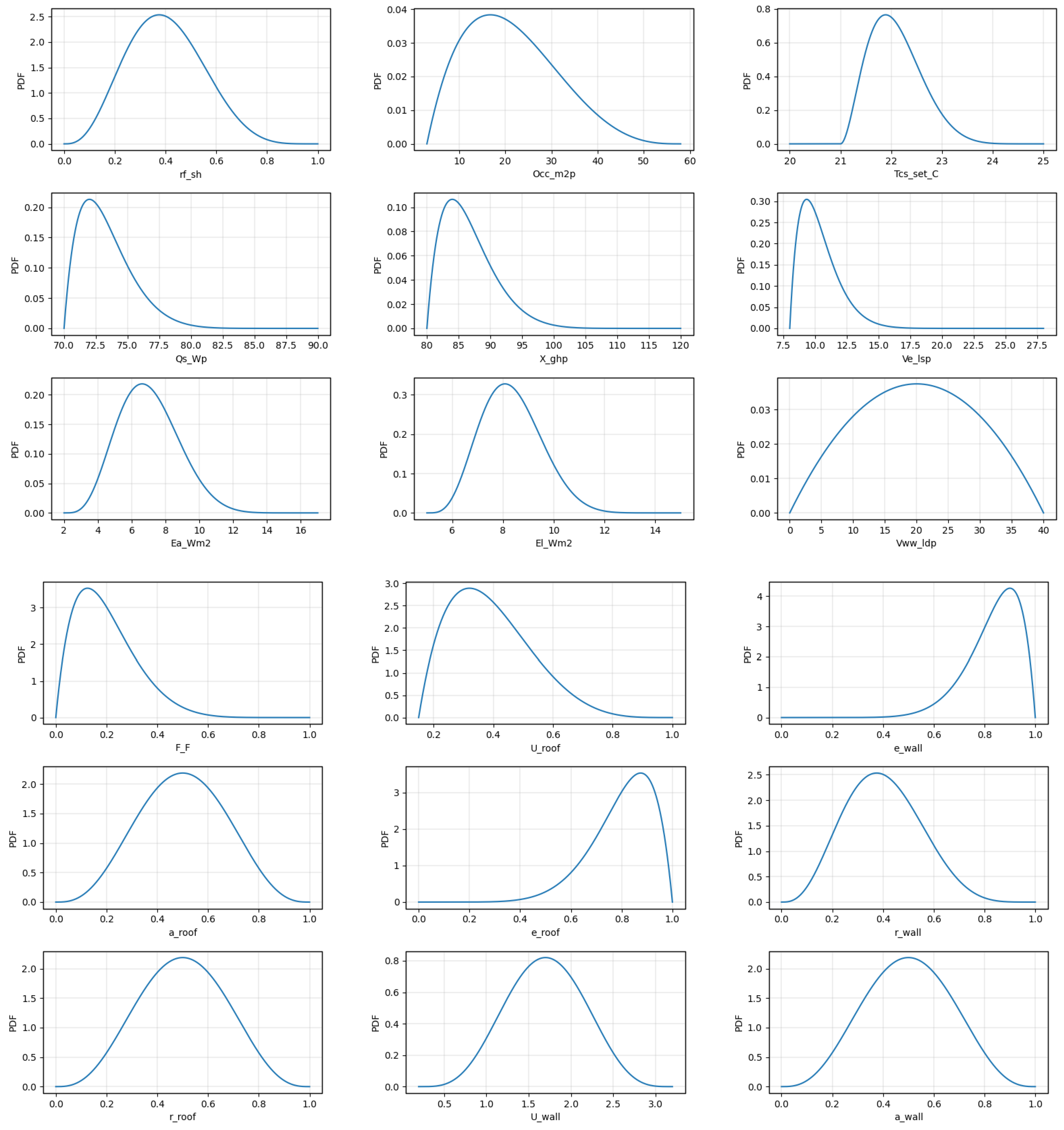
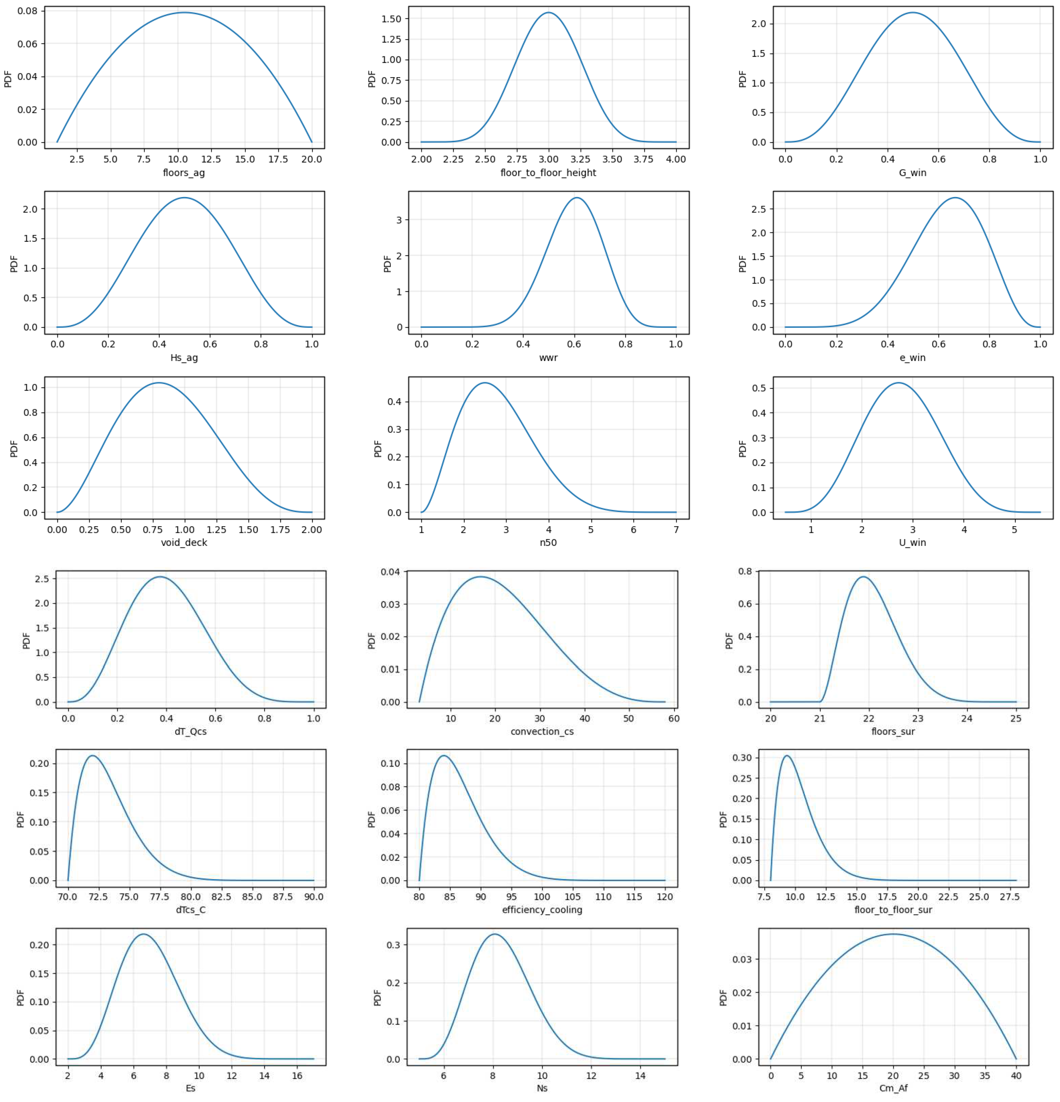
Each

x^{w}

parameter is considered as a realization of a random variable, according to a predefined Probability Density Function (PDF). We adopt a four-parameter (or generalized) beta distribution [26] based on distinct parameters for each input to steer the algorithm to explore the full expected range of parameter values while providing more samples for the section of values that is considered more likely to be observed. Appendix A indicates the distributions chosen for the 36 parameters.

A training dataset is generated by running the model for n times (in this study, 23,000 instances are used). At every instance, each one of the 36 variable inputs (

x^{w}

) generates a value stochastically via Monte Carlo technique, each based on their unique density and density parameters. The set of the generated inputs is then simulated by CEA, generating EUI as an output (

f (x^{P}, x_{i}^{w})

). The process is repeated in an automated manner until the full size of the dataset is achieved. With an input and output dataset, generated stochastically via the Monte Carlo method, we proceed with the implementation of the SM and estimation of its coefficients.

2.2. Surrogate Model development

This section introduces the principles of the SM, represented by

g (x^{w})

, such that:

\begin{matrix} f (x^{P}, x^{w}) = g (x^{w}) + ϵ, \end{matrix}

(3)

where

f (x^{P}, x^{w})

is the original (physics-based) model and

ϵ

is the discrepancy between

f (x^{P}, x^{w})

and

g (x^{w})

Given that

x^{P}

are static parameters, they are not encompassed by the SM, being interpreted as constants. While

g (x^{w})

can assume any form, we aim to propose one which is simple and provides mathematical tractability. Therefore, an MLR is proposed as the basis function for

g (x^{w})

\begin{matrix} g (x^{w}) & = β_{0} + β_{1} x_{1}^{w} + \dots + β_{K} x_{K}^{w} \end{matrix}

(4)

The MLR containing all the dataset

D

generated in the training phase can be formulated in a matrix form as follows:

[f = X β + ϵ,]

(5)

such that

f = [\begin{matrix} f_{1} \\ ⋮ \\ f_{n} \end{matrix}], X = [\begin{matrix} 1 & x_{11}^{w} & \dots & x_{1 K}^{w} \\ 1 & x_{21}^{w} & \dots & x_{2 K}^{w} \\ ⋮ & ⋮ & ⋱ & ⋮ \\ 1 & x_{n 1}^{w} & \dots & x_{n K}^{w} \end{matrix}], β = [\begin{matrix} β_{0} \\ ⋮ \\ β_{K} \end{matrix}], ϵ = [\begin{matrix} ϵ_{1} \\ ⋮ \\ ϵ_{n} \end{matrix}]

where:

$f \in R^{n}$ is a vector of observed values (dependent variable).
$X \in R^{n \times (K + 1)}$ is a matrix of row-vectors $x_{i}^{w}$ , which indicate the covariates (independent variables).
$β \in R^{K + 1}$ is a vector of regression coefficients.
$ϵ \in R^{n}$ is the error term vector.
$K \in N$ is the number of parameters.
$n \in N$ is size of the dataset.

In order to estimate the model coefficients, the Least Squares (LS) method is applied. This statistical technique aims to find the best fitting line (or plane, or hyperplane) for a set of data points by minimizing the sum of the squared differences of the error term vector (i.e., the difference between the observed values and the predicted values) of a linear regression model [27]. The optimal set of coefficients,

\hat{β}

, is calculated by solving the following objective:

\hat{β} = \underset{β}{arg min} {(f - X β)}^{T} (f - X β) .

(6)

The linear LS estimator is given by:

\hat{β} = {(X^{T} X)}^{- 1} X^{T} f .

(7)

The following algorithm summarizes the process to derive an MLR, given a training dataset:

Algorithm 2 Surrogate Model

1:: Inputs: $D$
2:: Outputs: model parameters $\hat{β}$
3:: Construct the design matrix:

$\begin{matrix} X = [\begin{matrix} 1 & x_{11}^{w} & \dots & x_{1 K}^{w} \\ 1 & x_{21}^{w} & \dots & x_{2 K}^{w} \\ ⋮ & ⋮ & ⋱ & ⋮ \\ 1 & x_{n 1}^{w} & \dots & x_{n K}^{w} \end{matrix}] \end{matrix}$
4:: Estimate model parameters:

$\hat{β} = {(X^{T} X)}^{- 1} X^{T} f$

With the model coefficients estimated, the model is now able to predict outputs based on a new set of inputs. In the next session, the accuracy of the SM developed is tested by comparing its performance with the original physics-based model (CEA), using a validation sample.

2.3. Validation Dataset generation

To guarantee generalization capabilities, the SM proposed is developed to be applicable to a whole population (i.e., all offices in Singapore). Therefore, the SM should be validated against a representative sample of this population, by comparing the outputs of the SM with CEA (Figure 3). The validation must be conducted on a dataset that has not been used during the training process, in order to prevent any potential biases and training contamination.

The training dataset consists of 25,000 samples and was generated by sampling the variable inputs (

x^{w}

) from four-parameter beta distributions and running CEA using those parameters as input.

In contrast, the validation dataset consists of 120 samples generated by running CEA on real-life buildings using calibrated values for the variable inputs and real-life data for the pre-defined variables (

x^{P}

). Figure 4 summarizes the differences between the training and the validation datasets.

The 120 office buildings used in the validation dataset are distributed over 5 commercial districts in Singapore. There is no available measured dataset that describes all inputs needed for those buildings, which would be required for this process. To address this limitation, we develop synthetic samples, generated artificially via computational modelling using CEA. The generated samples aim to "mimic" the real data.

The variable inputs for the modeled buildings (

x^{w}

) are calibrated to match the distribution of measured EUI data from 300 real office buildings in Singapore.

Pre-defined variables (

x^{P}

) for existing buildings are incorporated by extracting building footprints as described in Open Street Maps. Annual weather data is extracted from the closest available weather station from the study region. While those variables don’t have any impact on a trained SM, they are incorporated so that their variation and their possible impact on the outputs are still captured by the physics-based model (CEA).

After calibration, the EUI outputs for both the CEA model (assumed as ground truth value) and the SM are compared.

The calibration procedure consists of a Generator-Discriminator algorithm, inspired by Generative Adversarial Networks. The following algorithm indicates the process to generate the validation dataset:

Algorithm 3 Generator-Discriminator dataset generator

1:: Inputs: sample $y_{s} = {y_{s}^{i}}_{i = 1}^{M}$ , initial parameters $Φ$ , summary metric $S (\cdot)$ , distance metric $ρ (\cdot, \cdot)$ , threshold T.
2:: Outputs: set of calibrated inputs $x^{W}$
3:: Generate outputs $y_{s s}$ based on initial parameters $Φ$ .
4:: while $ρ (S (y_{s}), S (y_{s s})) \geq T$ do
5:: Generate inputs $x$ of the synthetic sample via Monte Carlo simulations, conditional on $Φ$ .
6:: Generate EUI for N synthetic samples ( $y_{s s} = {y_{s s}^{i}}_{i = 1}^{N}$ ) using the CEA ( $f (x^{P}, x^{w})$ ).
7:: Calculate non-parametric summaries (e.g., histograms) of the EUI for the sample ( $S (y_{s})$ ) and synthetic sample ( $S (y_{s s})$ ).
8:: Compare the summary statistics via a distance metric (e.g, Wasserstein metric) and obtain $ρ (S (y_{s}), S (y_{s s}))$ .
9:: Update the synthetic sample parameters by adding noise to the initial set of parameters $Φ = K Φ$ .
10:: end while
11:: The set of ${y_{s s}, x^{W}}$ is applied to the Surrogate Model ( $g (x^{w})$ ) and its error is compared to ( $f (x^{P}, x^{w})$ ).

The Generator model creates new candidate samples by changing the inputs of the model, which generates a distribution of EUI for the synthetic sample (

X_{s s}

) .

Meanwhile, the Discriminator model evaluates the quality of the generated samples by comparing the distribution of the model-generated outputs with observed sample data (

X_{s}

) from real office buildings in Singapore. The process is repeated until the convergence reaches a satisfactory threshold, evaluated via the Wasserstein distance.

The Wasserstein distance, commonly referred to also as the earth mover’s distance, is a distance metric which can be used to compare two probability distributions, including histograms. This method aims to find the least amount of work (i.e., "cost") required to move probability mass from one distribution to the other [28]. We adopt this method since it accounts for distances, which is represented as the bands on the EUI histogram. Therefore, a building with EUI closer to its expected value has lower cost than one with an EUI that is far from it. For one-dimensional metrics, the Wasserstein metric of the first order [29] is defined as:

\begin{matrix} W (S (y_{s s}), S (y_{s})) = \frac{1}{N} \sum_{i = 1}^{N} | | y_{s s_{i}} - {y_{s}}_{i} | |, \end{matrix}

(8)

where

N \in N^{+}

is the number of samples,

S (y_{s s})

is a vector composed of measurements from the synthetic samples

{y_{s s_{i}}, . . ., y_{s s_{N}}}

, and

S (y_{s})

is a vector composed of measurements from observations

{y_{s_{i}}, . . ., y_{s_{N}}}

We define as a threshold T for the Wasserstein distance the value of

22 k W h / m 2

, which, corresponds to

10 %

of the average of measured EUI. This value serves as a reference only and can be adjusted depending on how close the synthetic sample should be to the measurements, increasing the computational complexity as T decreases.

The result of the calibration, achieved after five iterations, is presented in Figure 5.

With a calibrated synthetic sample, the inputs from the validation dataset (

x^{w}

) are applied to the SM (

g (x^{w})

) and the output generated is compared to the one produced by CEA (

f (x^{P}, x^{w})

), measuring the error for each building. The results are presented in Section 3.

3. Results and Discussion

The model is trained (Section 2.1) with 23,000 instances of inputs/outputs by sampling 36 variable inputs according to distributions (Appendix A). The estimated coefficients of the linear regression (Section 2.2) are validated (Section 2.3) by comparing the SM with CEA for 120 calibrated buildings, assumed to be representative of all offices in Singapore.

In this section, we present and discuss the validation of the SM (Section 3.1). Furthermore, we analyse the model sensitivity through a normalized SM in order to perform variable selection (Section 3.2).

3.1. Validation Results

The error metrics obtained from the validation are presented in Table 1.

The error metrics provide an indication of how satisfactorily the SM is able to predict EUI when compared to the physics-based (CEA) model. The model is able to explain around 92.4% of the variation of data (

R^{2}

= 0.924). The mean absolute error (MAE = 7.38) is one to two orders of magnitude below the range of EUI predictions and, therefore, considerably small. A small normalized mean bias error is observed (NMBE = -3%), possibly due to the limitations of the SM to account for shading. The root mean squared error and its normalization (RMSE = 27.2, NRMSE = 13%, respectively) also indicate small uncertainties for the high ranges of EUI expected to be observed in office buildings.

In Figure 6 we present the goodness of fit between modeled and predicted EUI, and in Figure 7 we present the histogram of error, predominantly near zero.

The SM indicates a good prediction for offices according to the validation performed for 120 synthetically sampled buildings in Singapore. Although it was trained with limited interpretability about building footprint geometry and shading, this had little impact on the EUI, considering it is an annualized metric, normalized by gross floor area. Furthermore, it was able to perform well under distinct weather conditions, provided Singapore is a small country, with relatively homogeneous climate conditions, from a buildings’ energy perspective.

The SM is presented in Appendix B. A model sensitivity analysis is conducted (Section 3.2) to obtain interpretability about the most influential parameters and perform variable selection.

3.2. Model Sensitivity

A model sensitivity is conducted to analyse which inputs cause more variation of the outputs. The performance of a reduced order SM, based only on the most influential parameters, is analysed. For that, a normalized model is required, since each variable is expressed in different units and has different orders of magnitude. Therefore, we standardize (

μ = 0, σ = 1

) each variable of the training data in order to analyse the SM coefficients (

\hat{β}

) [20]:

Z = \frac{x - μ}{σ}

(9)

where: Z is the standardized variable, x is the original value of the variable,

μ

is the average value of a respective variable (in the dataset) and

σ

is the standard deviation (in the dataset).

The sensitivity of the parameters is evaluated according to the weights of the standardized MLR, presented in Table 2. The lowest values (blue) indicate the most influential with inverse correlation to EUI, while the highest values (red) indicate the most influential which are correlated to EUI.

The variables with the most influence are the internal loads, including: appliances and lighting (

E_{a}

and

E_{l}

, respectively), occupancy (

O c c

) and daily hot water consumption per person (

V_{w w}

Internal space usage also presents high influence, including the fraction of electrified (

E_{s}

), conditioned (

H_{s}

), and useful GFA spaces (

N_{s}

). HVAC properties such as its all-in-one efficiency (Eff) and temperature set points (

T_{c s}

) also have considerable effect.

Buildings’ thermal properties include most of the parameters, but most of them were revealed to have a small/ negligible impact on energy efficiency. Window-to-wall ratio (

w w r

) and thermal transmittance of the roof (

U_{r o o f}

) were the variables found to have a greater influence on the energy efficiency.

The original MLR with 36 parameters is compared to the reduced order SM, in which only the 11 most influential parameters are used in its training. The results are presented in Table 3.

The reduction in the number of parameters does not impact model performance, probably due to reduced influence and high correlation from some of the variables, such that the remaining variables are able to capture behaviour which would be explained for the eliminated ones. Therefore, the reduced order SM is recommended as a suitable option to represent the EUI of a generic office building. The reduced order SM is presented below:

\begin{matrix} \begin{matrix} E U I = & - 21.927 + 56.625 H_{s} + 126.190 E_{s} + 79.030 N_{s} + 28.589 w w r + 29.991 U_{r o o f} \\ - 1.628 O c c + 4.620 E_{a} + 4.868 E_{l} + 1.029 V_{w w} - 4.274 T_{c s} - 13.527 E f f \\ + ε_{S M} + ε_{C E A}, \end{matrix} \end{matrix}

(10)

where:

H_{s}

: fraction of conditioned spaces

E_{s}

: fraction of electrified spaces

N_{s}

: fraction of useful GFA

w w r

: window-to-wall ratio

U_{r o o f}

: Thermal transmittance of the roof (

W / m^{2} K

)

O c c

: Peak occupancy ratio (

m^{2} / p

)

E_{a}

: Peak electrical load from appliances (

W / m^{2}

)

E_{l}

: Peak electrical load from lighting (

W / m^{2}

)

V_{w w}

: Volume of hot water (

l d p

)

T_{c s}

: Temperature set point for cooling (

ˆ \circ

E f f

: Overall efficiency of the cooling system

ε_{S M}

: surrogate model error (in relation to CEA)

ε_{C E A}

: CEA error (in relation to reality).

This simple, yet comprehensive, model is considered suitable for all existing office buildings in Singapore. Hypothetical offices, such as the ones resulting from retrofitting of current offices or newly developed sites can also be tested with no foreseen impact on the accuracy of the model. In line with that, we present an example of application for the SM in Section 4.

4. Application of the Surrogate Model

In this section, we use an illustrative example to demonstrate how the SM can be used to evaluate practical problems that presents additional computational challenges when evaluated via physics-based models.

In this particular example, we take uncertainty into account while evaluating assumed current and hypothetical future scenarios in the context of Singapore. In Singapore, the energy efficiency landscape is closely related to a Super Low Energy (SLE) programme, which requires buildings to provide at least 60% energy savings over the 2005 building code or to have EUIs under specific benchmark values. For office spaces, the benchmark for SLE buildings is defined by

E U I \leq

100

k W h / m^{2} y r

(small offices) and

E U I \leq

115

k W h / m^{2} y r

(large offices) [30], therefore 100

k W h / m^{2} y r

is used as the threshold for this analysis.

For an observed building, with inputs that follow a given distribution, we aim to determine:

What is the probability it meets the SLE criteria? (Baseline scenario)
How may a roadmap of improvements change this probability? (What-if scenario)

We assume each building parameter to be a random variable which follows a normal distribution with a known mean and variance. For the baseline case, this information can be derived from on-site energy audits and building surveys with the owners, developers and tenants. Given practical constraints, those values could not be obtained. Therefore, assumptions which use professional expertise are carried out to enable this illustration exercise. For the what-if scenario, we assume a series of measures is implemented, which improves, on average, how buildings are designed and operated. The provided inputs for the baseline case and what-if scenario are indicated in Table 4. For this case, the uncertainty (error) caused by the SM (

ε_{S M}

) is derived from the validation (Section 3.1), assuming the mean error to be zero (non-bias) and variance to be the previously calculated MSE (

μ = 0, σ = 729

). In this example, the uncertainty from the physics-based model (

ε_{C E A}

) is not considered (

μ = 0, σ = 0

Therefore, the probabilities of the EUI are the result of applying the observed properties into the reduced order SM. The results for each scenario can be analysed via probability density functions (PDF) and cumulative distribution functions (CDF), as presented in Figure 8.

For the baseline case, the EUI has an expected mean of 227

k W h / m^{2}

and standard deviation of

42.3

k W h / m^{2}

. In this distribution, the probability of a given sampled building to meet the benchmark (

E U I \leq 100 k W h / m^{2} y r

) is 0.14%. For the what-if case, after measures have been implemented, the EUI has an expected mean of 99

k W h / m^{2}

and standard deviation remained

42.3

k W h / m^{2}

, since the uncertainty for each input parameter was not changed. In this distribution, the probability of a given sampled building to meet the benchmark (

E U I \leq 100 k W h / m^{2} y r

) is 51%, significantly increasing the likelihood of SLE buildings to be observed.

While this analysis is merely for illustrative purposes, to highlight the surrogate model’s capabilities, this analysis may assist to provide a possible roadmap for the increase of energy efficiency in office buildings, applied to the Singaporean context. Nonetheless, more thorough data collection and analysis is suggested to extend the conclusions of this example to the real world.

5. Conclusions

We developed a Multiple Linear Regression (MLR) Surrogate Model (SM) of a physics-based model, City Energy Analyst (CEA), to predict office buildings’ Energy Use Intensity (EUI) in the context of Singapore. The SM is based on 36 independent input parameters, which encompass thermal properties of building materials, internal space usage, properties of the HVAC system, and internal loads.

The SM is trained with

23, 000

input/output samples, which are obtained by running CEA stochastically. For each instance, a set of inputs is generated via Monte Carlo simulations based on four-parameter beta distributions. This set is then applied in a building energy simulation, with predefined weather, building footprint, and schedules, accounting for computational and model limitations.

The trained model is then validated against a wide range of office buildings in Singapore, representative of the population. The validation dataset is based on synthetic samples, generated by a Generator-Discriminator algorithm, which calibrates 120 buildings observed in Singapore to reported EUI data. Although the SM was trained with limited interpretability about building footprint geometry, shading and weather conditions, the validation aimed to account for all those in a more realistic manner, exploring all the complexity and heterogeneity observed in this population. This ensures the model can be used for more general uses, without expecting further decrease in its accuracy.

The results indicate a good agreement of the predictions of the surrogate when compared to the outputs provided by the physics-based model. The validation indicated an

R^{2}

of 0.924, an NMBE of -3% and an NRMSE of 13%.

Model sensitivity indicates that the internal loads and overall internal space usage are the categories that have the largest influence on the energy efficiency. When evaluating a reduced order SM, accounting for only the 11 most influential parameters, the impact on performance was negligible. This can possibly be explained due to the reduced influence of variables removed and high correlation between variables. Therefore, the reduced order SM is recommended as a suitable option to represent the EUI of generic office buildings.

The proposed SM can be applied to all existing and hypothetical offices (e.g., planned retrofits and new developments) in Singapore. It is suitable for analysis where wide exploration of the parameter space is often required (e.g., design optimization, sensitivity analysis and what-if analysis). Furthermore, it is useful whenever computational costs need to be minimized (e.g., large-scale simulations) or when uncertainty should be considered (e.g., early-stage design).

A new SM should be trained for different climate conditions (e.g., other countries or Singapore in 50 years) and different building usages (e.g., residential, offices with atypical hours). Although the model was developed for a specific context (Office buildings for the current climate of Singapore), the framework can easily be adapted to consider other climates, building types, and physics-based models.

Future work expects to test wider implementation of the SM in different setups (e.g., different countries and for different building types). Different SM structures besides the statistical MLR developed, such as machine learning techniques (e.g., artificial neural network), can be tested to explore the capability of achieving even higher performance. Finally, given the flexibility and low-computational expenses of the SM, more complex applications can be explored, which would not be suitable for physics-based models.

Author Contributions

Conceptualization, L.G.R.S. and I.N.; methodology, L.G.R.S., I.N, J.I., M.N.; software, L.G.R.S.; validation, L.G.R.S., I.N., J.I.; formal analysis, L.G.R.S., I.N.; investigation, L.G.R.S.; resources, I.N.; data curation, L.G.R.S.; writing—original draft preparation, L.G.R.S., I.N.; writing—review and editing, I.N., J.I., M.,N.; visualization, L.G.R.S.; supervision, I.N., J.I.; project administration, I.N., J.I.; funding acquisition, I.N. All authors have read and agreed to the published version of the manuscript.

Funding

This research was funded by Singapore’s National Research Foundation (NRF) under its Virtual Singapore programme.

Institutional Review Board Statement

Not applicable

Informed Consent Statement

Not applicable

Data Availability Statement

Data and codes related to this work can be found at: https://github.com/cooling-singapore/EnergyEfficiency. Please contact authors for additional information regarding data availability.

Acknowledgments

The research was conducted under the Cooling Singapore project, funded by Singapore’s National Research Foundation (NRF) under its Virtual Singapore programme. Cooling Singapore is a collaborative project led by the Singapore-ETH Centre (SEC), with the Singapore-MIT Alliance for Research and Technology (SMART), TUMCREATE (established by the Technical University of Munich), the Cambridge Centre for Advanced Research and Education in Singapore (CARES), the National University of Singapore (NUS), the Singapore Management University (SMU), and the Agency for Science, Technology and Research (A*STAR).

Conflicts of Interest

The authors declare no conflict of interest.

Appendix A

Here we present the (generalized) beta distribution for each input parameter, used to generate data to train the model in Section 2.1. The description of each variable and their units is presented Appendix B.

Appendix B

Here we present the full order Surrogate Model (SM), evaluated in Section 3.1:

\begin{matrix} \begin{matrix} E U I = & - 128.163 - 0.116 n_{f l o o r : r e f} + 3.922 h_{f l o o r : r e f} + 0.007 n_{f l o o r s : s u r} - 0.699 h_{f l o o r : s u r} \\ + 57.115 H s + 119.518 E s + 72.369 N s + 0.531 v o i d_d e c k + 24.266 w w r \\ + 1.73 \times 10^{- 6} C m_A f + 0.410 n 50 + 3.159 U_{w i n} - 0.218 e_{w i n} + 11.673 F_F \\ + 26.024 U_{r o o f} + 2.784 a_{r o o f} - 0.801 e_{r o o f} - 0.373 r_{r o o f} + 2.275 U_{w a l l} + 7.295 G_{w i n} \\ + 2.050 a_{w a l l} - 2.410 e_{w a l l} - 0.051 r_{w a l l} + 8.829 r f_{s h} - 1.626 O c c + 0.720 Q s \\ + 0.353 X + 5.032 E a + 5.284 E l + 1.015 V w w - 4.809 T_{c s} + 1.624 V e \\ - 1.940 d T_{Q c s} - 4.647 c o n v - 1.861 d T c s_{C} - 13.825 E f f + ε_{S M} + ε_{C E A} \end{matrix} \end{matrix}

Where:

Table A1. Parameters of CEA incorporated into the SM

Parameter	Units	Description
n_floor_ref	-	Number of floors (ref. building)
h_floor_ref	m	Floor height (ref. building)
n_floors_sur	-	Number of floors (surrounding buildings)
h_floor_sur	m	Floor height (surrounding buildings)
Hs	-	Percentage of conditioned spaces
Es	-	Percentage of electrified spaces
Ns	-	Percentage of useful gross floor area
void_deck	-	Number of floors which are void decks
wwr	-	Window to wall ratio
Cm_Af	J/km2	Internal heat capacity per unit of air conditioned area
n50	1/h	Air exchanges per hour at a pressure of 50 Pa
U_win	W/m2.K	Thermal transmittance of windows
G_win	-	Solar heat gain coefficient
e_win	-	Emissivity for windows
F_F	-	Frame fraction for windows
U_roof	W/m2.K	Thermal transmittance of the roof
a_roof	-	Solar absorption coefficient for roof
e_roof	-	Emissivity for roof
r_roof	-	Thermal reflectance for roof
U_wall	W/m2.K	Thermal transmittance of walls
a_wall	-	Solar absorption coefficient for walls
e_wall	-	Emissivity for walls
r_wall	-	Thermal reflectance for walls
rf_sh	-	Shading coefficient
Occ	m2/p	Occupancy density
Qs	W/p	Peak sensible heat load of people
X	ghp	Moisture released by occupancy at peak conditions
Ea	W/m2	Peak electricity for appliances
El	W/m2	Peak electricity for lighting
Vww	l/d/p	Peak specific daily hot water consumption
T_cs	C	Temperature set point for cooling
Ve	l/s/p	Minimum outdoor air ventilation rate for Air Quality
dT_Qcs	C	Correction temperature of emission losses
conv	-	Convective ratio in relation to the total power
dTcs_C	C	Set-point correction for space emission systems
Eff	-	Efficiency of the all-in-one cooling system

References

IEA. Buildings. Technical report, IEA, Paris, 2022. https://www.iea.org/reports/buildings, License: CC BY 4.0.
Berardi, U. A cross-country comparison of the building energy consumptions and their trends. Resources, Conservation and Recycling 2017, 123, 230–241. [CrossRef]
Li, D.H.; Yang, L.; Lam, J.C. Impact of climate change on energy use in the built environment in different climate zones – A review. Energy 2012, 42, 103–112. 8th World Energy System Conference, WESC 2010. [CrossRef]
Hu, S.; Yan, D.; Azar, E.; Guo, F. A systematic review of occupant behavior in building energy policy. Building and Environment 2020, 175, 106807.
Jones, A. Indoor air quality and health. Atmospheric Environment 1999, 33, 4535–4564. [CrossRef]
Nicol, J.F.; Humphreys, M.A. Adaptive thermal comfort and sustainable thermal standards for buildings. Energy and buildings 2002, 34, 563–572.
Kleerekoper, L.; van Esch, M.; Salcedo, T.B. How to make a city climate-proof, addressing the urban heat island effect. Resources, Conservation and Recycling 2012, 64, 30–38. Climate Proofing Cities. [CrossRef]
Cabeza, L.F.; Palacios, A.; Serrano, S.; Ürge Vorsatz, D.; Barreneche, C. Comparison of past projections of global and regional primary and final energy consumption with historical data. Renewable and Sustainable Energy Reviews 2018, 82, 681–688. [CrossRef]
Lam, J.C.; Hui, S.C. Sensitivity analysis of energy performance of office buildings. Building and Environment 1996, 31, 27–39. [CrossRef]
Sozer, H. Improving energy efficiency through the design of the building envelope. Building and Environment 2010, 45, 2581–2593. [CrossRef]
Gaetani, I.; Hoes, P.J.; Hensen, J.L. Estimating the influence of occupant behavior on building heating and cooling energy in one simulation run. Applied Energy 2018, 223, 159–171. [CrossRef]
Mustafaraj, G.; Marini, D.; Costa, A.; Keane, M. Model calibration for building energy efficiency simulation. Applied Energy 2014, 130, 72–85. [CrossRef]
Rocha, P.; Siddiqui, A.; Stadler, M. Improving energy efficiency via smart building energy management systems: A comparison with policy measures. Energy and Buildings 2015, 88, 203–213. [CrossRef]
Guo, S.; Yan, D.; Hu, S.; Zhang, Y. Modelling building energy consumption in China under different future scenarios. Energy 2021, 214, 119063. [CrossRef]
Dong, B.; Lee, S.E.; Sapar, M.H. A holistic utility bill analysis method for baselining whole commercial building energy consumption in Singapore. Energy and Buildings 2005, 37, 167–174. [CrossRef]
Dong, B.; Cao, C.; Lee, S.E. Applying support vector machines to predict building energy consumption in tropical region. Energy and Buildings 2005, 37, 545–553. [CrossRef]
Casella, G.; Berger, R. Statistical Inference; Cengage Learning, 2021.
Yalcintas, M.; Akkurt, S. Artificial neural networks applications in building energy predictions and a case study for tropical climates. International Journal of Energy Research 2005, 29, 891–901, [https://onlinelibrary.wiley.com/doi/pdf/10.1002/er.1105]. [CrossRef]
Yalcintas, M. An energy benchmarking model based on artificial neural network method with a case example for tropical climates. International Journal of Energy Research 2006, 30, 1158–1174, [https://onlinelibrary.wiley.com/doi/pdf/10.1002/er.1212]. [CrossRef]
Mottahedi, M.; Mohammadpour, A.; Amiri, S.S.; Riley, D.; Asadi, S. Multi-linear Regression Models to Predict the Annual Energy Consumption of an Office Building with Different Shapes. Procedia Engineering 2015, 118, 622–629. Defining the future of sustainability and resilience in design, engineering and construction. [CrossRef]
Melo, A.; Versage, R.; Sawaya, G.; Lamberts, R. A novel surrogate model to support building energy labelling system: A new approach to assess cooling energy demand in commercial buildings. Energy and Buildings 2016, 131, 233–247. [CrossRef]
Papadopoulos, S.; Azar, E. Integrating building performance simulation in agent-based modeling using regression surrogate models: A novel human-in-the-loop energy modeling approach. Energy and Buildings 2016, 128, 214–223. [CrossRef]
Norford, L.; Socolow, R.; Hsieh, E.; Spadaro, G. Two-to-one discrepancy between measured and predicted performance of a ‘low-energy’ office building: insights from a reconciliation based on the DOE-2 model. Energy and Buildings 1994, 21, 121–131. [CrossRef]
Ryan, E.M.; Sanquist, T.F. Validation of building energy modeling tools under idealized and realistic conditions. Energy and Buildings 2012, 47, 375–382. [CrossRef]
Fonseca, J.A.; Nguyen, T.A.; Schlueter, A.; Marechal, F. City Energy Analyst (CEA): Integrated framework for analysis and optimization of building energy systems in neighborhoods and city districts. Energy and Buildings 2016, 113, 202–226.
McDonald, J.B.; Xu, Y.J. A generalization of the beta distribution with applications. Journal of Econometrics 1995, 66, 133–152. [CrossRef]
Åke Björck. Least squares methods. In Handbook of Numerical Analysis; Elsevier, 1990; Vol. 1, Handbook of Numerical Analysis, pp. 465–652. [CrossRef]
Vallender, S.S. Calculation of the Wasserstein Distance Between Probability Distributions on the Line. Theory of Probability & Its Applications 1974, 18, 784–786, [https://doi.org/10.1137/1118101]. [CrossRef]
Villani, C. Topics in Optimal Transportation; Graduate studies in mathematics, American Mathematical Society, 2003.
BCA. Green Mark SLE: Super Low Energy Buildings. Building Construction Authority, 2021.

Figure 1. Workflow of development (Section 2) and evaluation (Section 3.1) of the proposed SM, evaluation of the model sensitivity (Section 3.2) and case study analysis (Section 4).

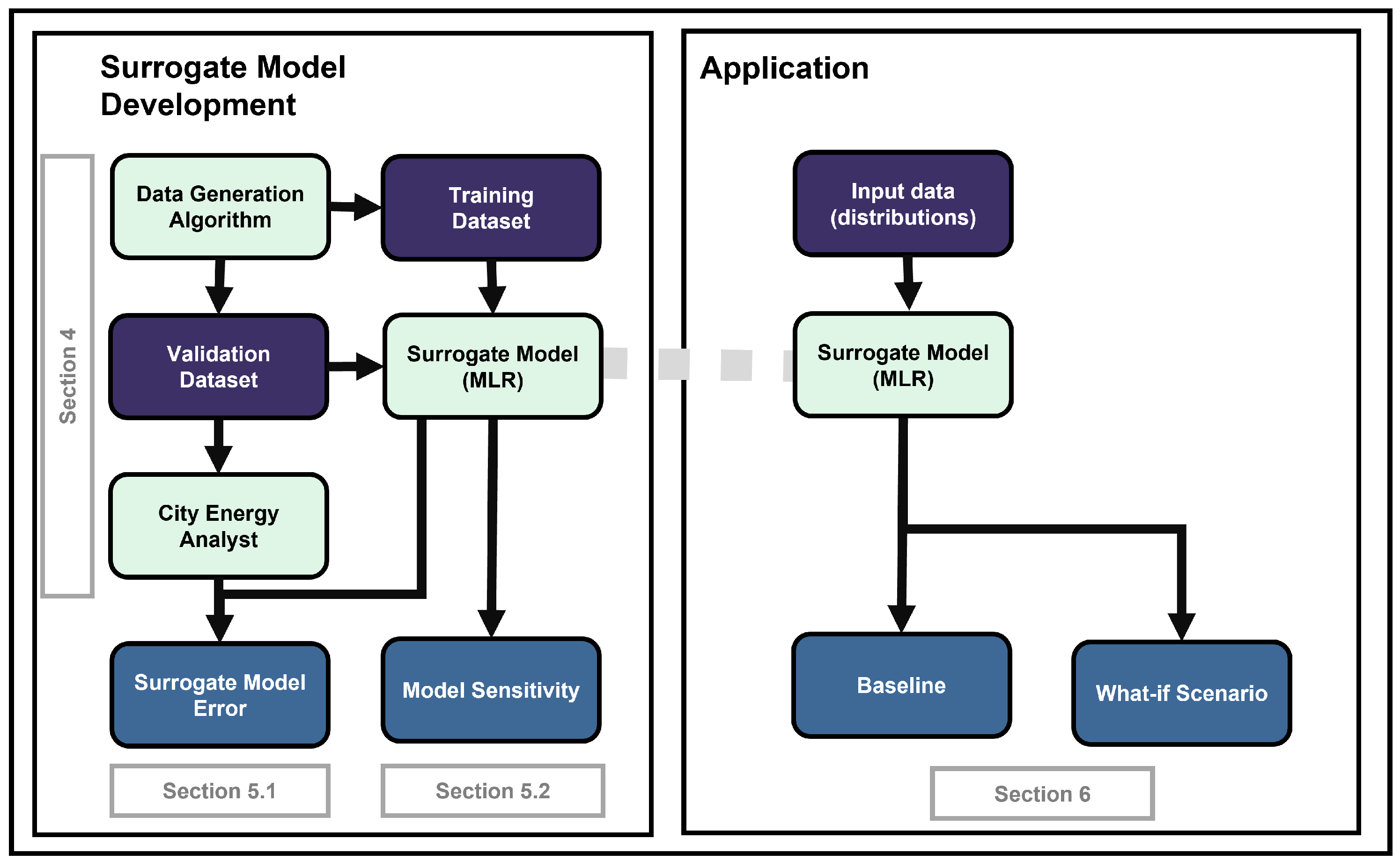
Figure 2. Summary of the training process to develop the SM

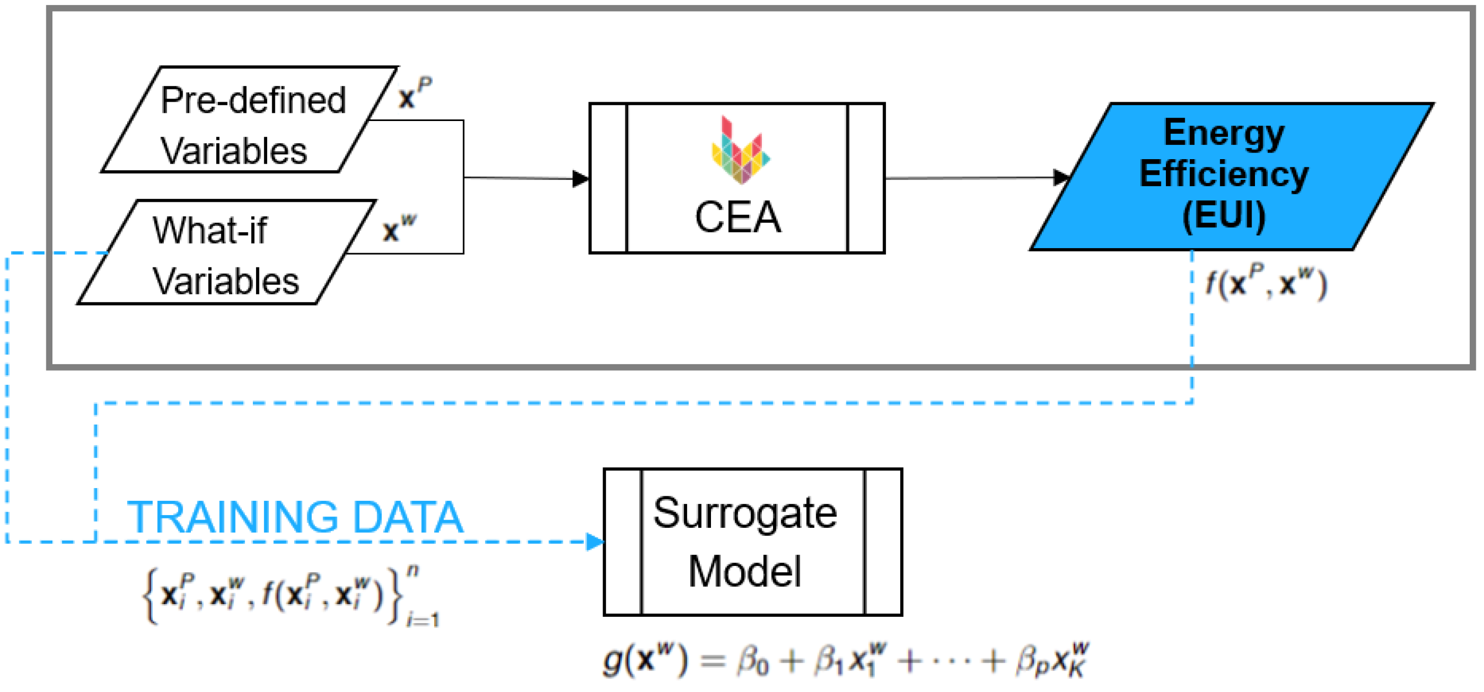
Figure 3. Summary of the validation process to estimate the error of the SM

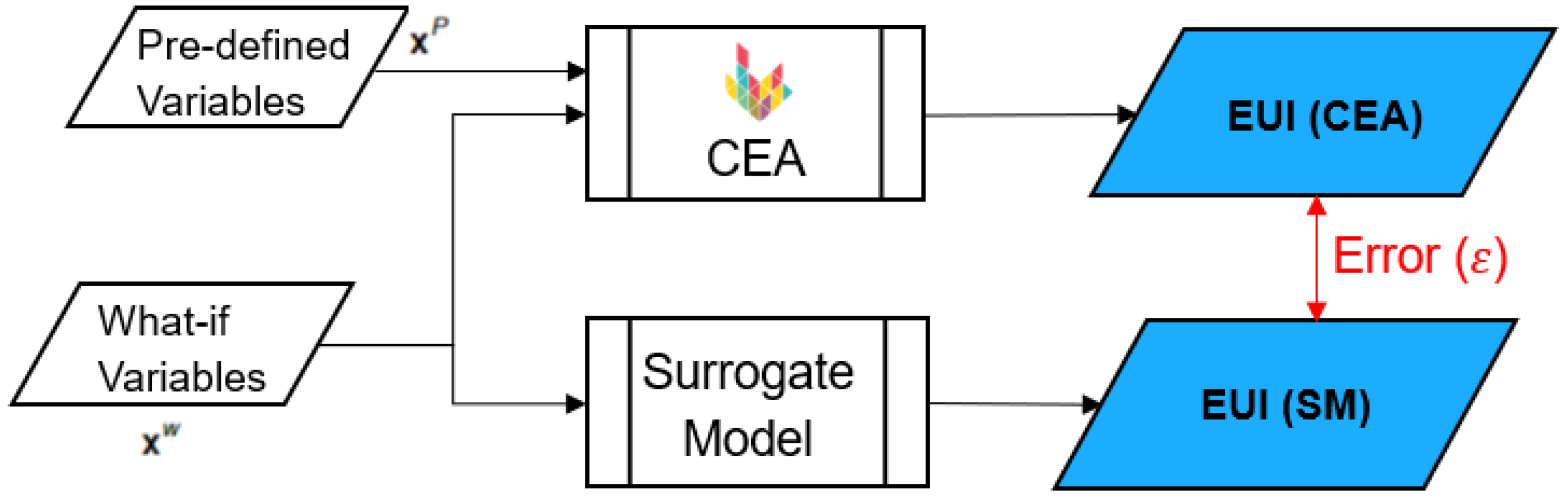
Figure 4. Summary of the training and validation dataset. Red indicated unchanged parameters, while blue indicates changed parameters.

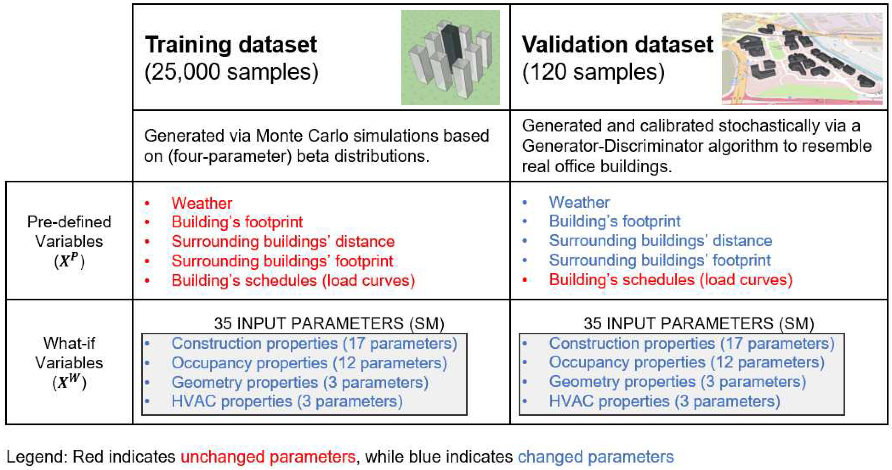
Figure 5. Histogram of calibrated modeled buildings from the synthetic sample (left) compared to reported data from a population sample (right).

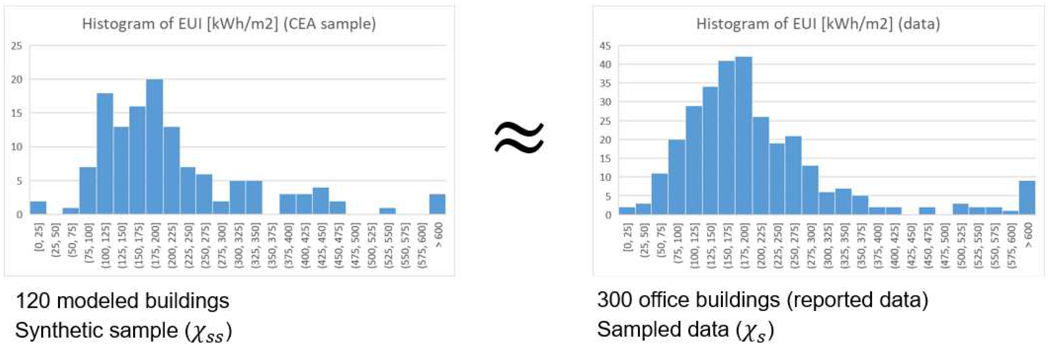
Figure 6. The x-axis indicates the expected "true" values (modeled and simulated by CEA), while the y-axis indicates the simulated values (from the SM).

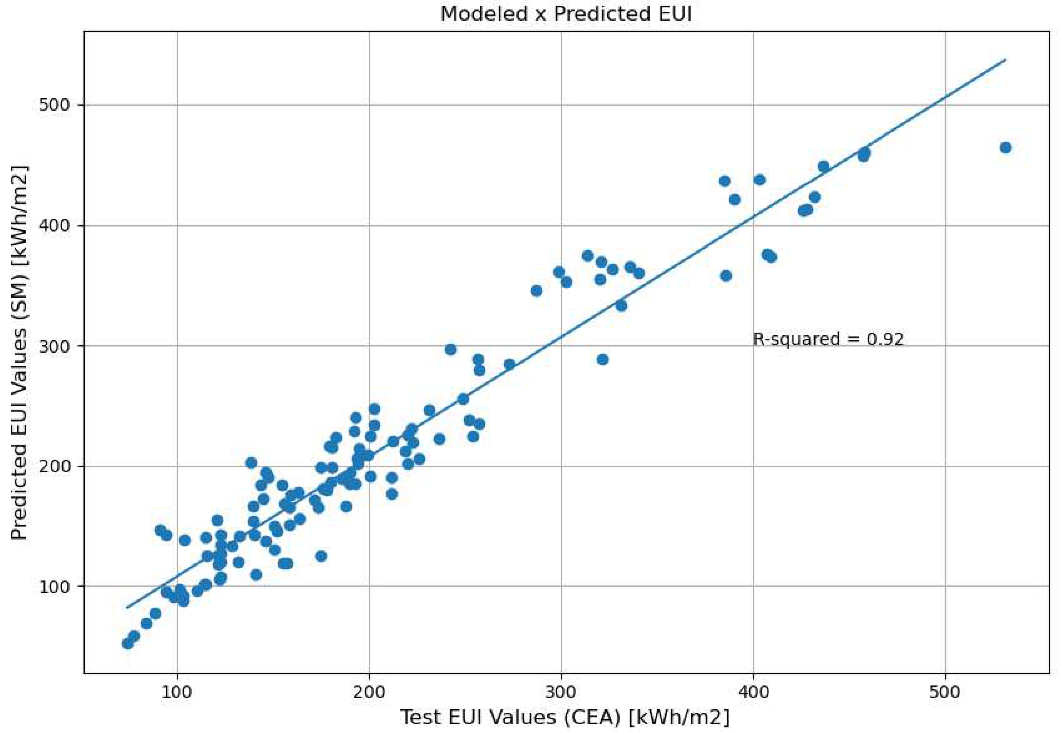
Figure 7. Histogram of the error, which is measured by the relative difference of the SM and the CEA model.

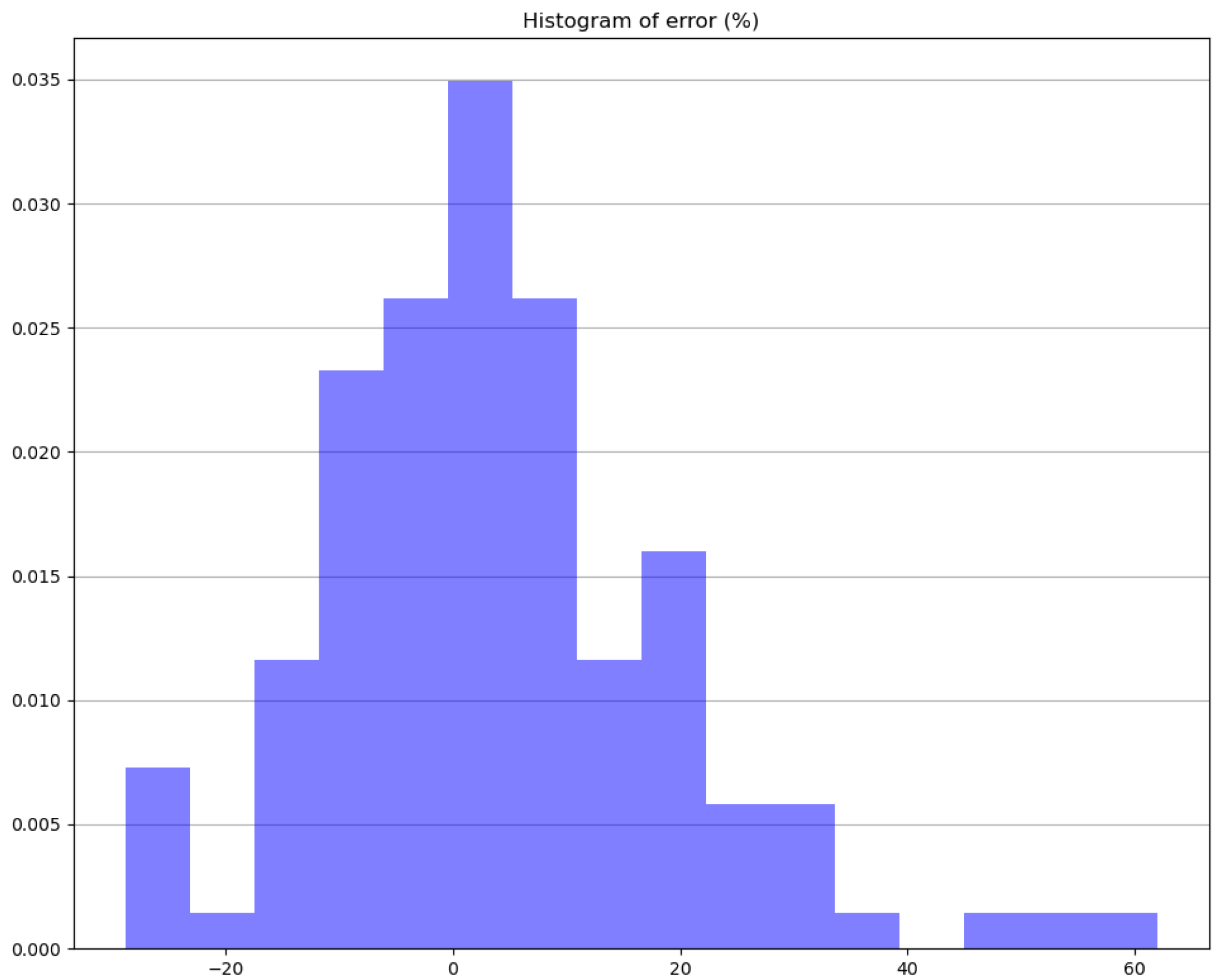
Figure 8. Probability density functions (left) and cumulative distribution functions (right) for the baseline (top, blue) and what-if scenario (bottom, green)

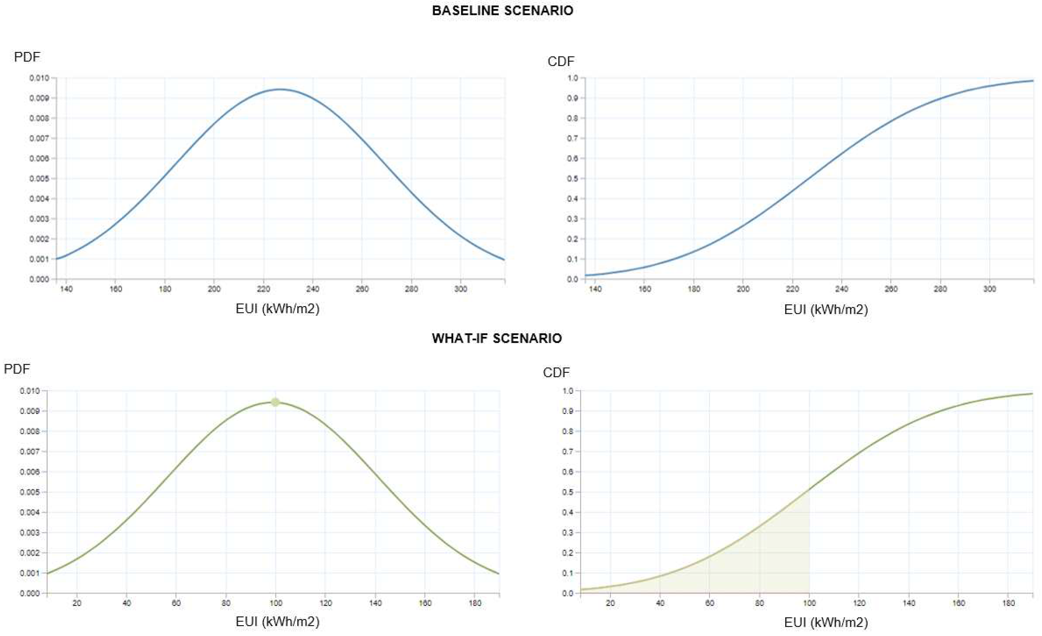
Table 1. Error metrics for surrogate model validation

$R^{2}$	MAE	NMBE	RMSE	NRMSE
0.924	7.38	-3.56%	27.2	13.13%

Table 2. Model sensitivity is evaluated by the weights of a standardized model.

Variable Name	Coefficient	Variable Name	Coefficient	Variable Name	Coefficient
Occ	-13.1642	Intercept	0	Qs_Wp	2.4557
Eff	-6.4138	surrounding_floors	0.0278	Ve_lsp	2.4675
Tcs	-5.4897	Cm_Af	0.0473	U_win	2.556
dT_Qcs	-0.5894	void_deck	0.2294	wwr	3.2396
convection	-0.5031	a_wall	0.342	Ns	6.6854
floors	-0.4946	n50	0.3578	U_roof	7.0703
e_wall	-0.2487	a_roof	0.4649	Vww_ldp	9.3365
surroundings_floor_height	-0.1697	floor_height	0.9547	Hs_ag	9.6704
e_roof	-0.0967	U_wall	0.9976	Es	13.2444
dTcs_C	-0.0706	G_win	1.2137	El_Wm2	22.8745
r_roof	-0.0621	rf_sh	1.3	Ea_Wm2	25.1245
e win	-0.0302	FF	1.4631
r_wall	-0.0076	X_ghp	1.8171

Table 3. Comparison of full and reduced order models.

Number of parameters	$R^{2}$	MAE	NMBE	RMSE	NRMSE
Full model (36 parameters)	0.924	7.38	-3.56%	27.2	13.13%
Reduced order model (11 parameters)	0.925	5.36	-2.59	26.9	12.99%

Table 4. Derived distribution for each parameter for the baseline (left) and what-if (right) scenarios. Blue indicate the changes.

Baseline		What-if Scenario
$H_{s} \sim N (0.8, 0.01)$	$E_{l} \sim N (15, 16)$	$H_{s} \sim N (0.6, 0.01)$	$E_{l} \sim N (7, 16)$
$E_{s} \sim N (0.9, 0.0025)$	$V_{w w} \sim N (7, 4)$	$E_{s} \sim N (0.9, 0.0025)$	$V_{w w} \sim N (4, 4)$
$N_{s} \sim N (1, 0)$	$T_{c s} \sim N (23, 1)$	$N_{s} \sim N (1, 0)$	$T_{c s} \sim N (24, 1)$
$w w r \sim N (0.7, 0.01)$	$E f f \sim N (3.5, 1)$	$w w r \sim N (0.5, 0.01)$	$E f f \sim N (5, 1)$
$U_{r o o f} \sim N (0.4, 0.04)$	$ε_{S M} \sim N (0, 729)$	$U_{r o o f} \sim N (0.15, 0.04)$	$ε_{S M} \sim N (0, 729)$
$O c c \sim N (15, 9)$	$ε_{C E A} \sim N (0, 0)$	$O c c \sim N (15, 9)$	$ε_{C E A} \sim N (0, 0)$
$E_{a} \sim N (15, 16)$		$E_{a} \sim N (7, 16)$

Disclaimer/Publisher’s Note: The statements, opinions and data contained in all publications are solely those of the individual author(s) and contributor(s) and not of MDPI and/or the editor(s). MDPI and/or the editor(s) disclaim responsibility for any injury to people or property resulting from any ideas, methods, instructions or products referred to in the content.

© 2024 by the authors. Licensee MDPI, Basel, Switzerland. This article is an open access article distributed under the terms and conditions of the Creative Commons Attribution (CC BY) license (http://creativecommons.org/licenses/by/4.0/).

Copyright: This open access article is published under a Creative Commons CC BY 4.0 license, which permit the free download, distribution, and reuse, provided that the author and preprint are cited in any reuse.

Downloads

114

Views

Comments

Subscription

Notify me about updates to this article or when a peer-reviewed version is published.

MDPI Initiatives

Important Links

Choose an area of interest and we will send you notifications of new preprints at your preferred frequency.

Disclaimer

Estimation of Buildings’ Energy Efficiency via a Surrogate Regression Model

Abstract

Keywords:

Subject:

1. Introduction

1.1. Literature Review

1.2. Applications

1.3. Contributions

1.4. Paper organisation

2. Methodology

2.1. Training Dataset generation

2.2. Surrogate Model development

2.3. Validation Dataset generation

3. Results and Discussion

3.1. Validation Results

3.2. Model Sensitivity

4. Application of the Surrogate Model

5. Conclusions

Author Contributions

Funding

Institutional Review Board Statement

Informed Consent Statement

Data Availability Statement

Acknowledgments

Conflicts of Interest

Appendix A

Appendix B

References

MDPI Initiatives

Important Links

Subscribe