
Submitted:
18 January 2024
Posted:
19 January 2024
You are already at the latest version
Abstract
This research paper presents a comprehensive study on the gasification of wheat straw pellets in a 10-kW fixed bed gasifier through a combination of Computational Fluid Dynamics (CFD) simulation and experimental validation. The developed 2D CFD model in ANSYS meshing simulates the gasification process in ANSYS Fluent software. The investigation evaluates key parameters such as equivalence ratio, higher heating value, and temperature distribution within the gasifier to enhance syngas production efficiency. The simulated results exhibit a noteworthy agreement with experimental data obtained from gasification. The impact of the equivalence ratio on gas production and lower heating value (LHV) is systematically explored, revealing that an equivalence ratio of 0.35 is optimal for syngas production. The resulting producer gas composition at this optimum condition includes CO (~27.67%), CH4 (~3.29%), CO2 (~11.09%), H2 (~11.09%), and N2 (~51%). The study further investigates the positive influence of reactor temperature on increasing syngas quantity while considering the uneven shape of the reactor and various thermal reactions affecting temperature, static pressure, velocity, and density. The findings contribute valuable insights to improve the efficiency of fixed-bed gasifiers, offering essential information on performance parameters for sustainable and optimized syngas production.
Keywords:
biomass
; downdraft gasifier
; syngas
; computational fluid dynamics
; simulation
; wheat straw pellets
1. Introduction
Biomass is a reliable source of alternative energy used in both developed and developing countries, playing a significant role in global power generation [1]. However, directly using biomass for energy production is often inefficient. So, a preferred method is to convert biomass into the desired fuel [2,3]. Various technologies, like combustion, gasification, and pyrolysis, have been developed for this purpose [4]. Gasification, in particular, is a common method with a high efficiency of up to 50% [5]. Downdraft gasification is a promising technology for turning compacted biomass into energy, especially suitable for smaller to medium-scale power generation [6].
Gasification is more complex than combustion and pyrolysis because it involves a series of chemical reactions in a pyrolytic process [7]. As a result, findings from laboratory-scale gasification experiments are often inconclusive. Additionally, designing appropriately sized gasifiers is a challenging task that demands significant effort and resources. Moreover, the process is time-consuming and requires substantial experimental facilities [2]. However, employing a numerical method proves to be an efficient way to gain insights into the gasification process and understand the fundamental physics involved. Modeling approaches are cost-effective, saving time, budget, and resources, while also facilitating repeatability and justifiable modifications when needed. Various numerical models and simulation tools, including thermodynamic equilibrium, kinetics, computational fluid dynamics (CFD), artificial neural networks (ANN), and ASPEN plus, have been utilized for gasification in downdraft reactors [6,8,9,10,11].
Among various modeling techniques, Computational Fluid Dynamics (CFD) is considered the most suitable for simulating and predicting the gasification process in fixed-bed gasifiers due to its ease of operation [11,12]. Many prefer CFD for both scientific research and engineering applications because of its versatility [13]. The CFD model utilizes mass-energy balance and dynamic chemical reactions, enabling it to predict the temperature distribution profile within the gasification zone [14,15]. One significant advantage of CFD models is their ability to provide accurate estimations of temperature and gas yield throughout the entire reactor [16]. Additionally, CFD models are well-suited for handling dense particulate matter, such as pellets [17]. Researchers have created two-dimensional (2D) CFD simulations for both updraft and downdraft gasifiers in the gasification process [1,14,18,19]. A review by Patra and Sheth [9] highlighted the challenges of CFD modeling specifically in downdraft gasifiers, indicating that additional effort is needed to address these issues. Therefore, more effort is required to solve the problems. Baruah and Baruah [8] in their literature review, emphasized the significance of CFD simulations for biomass gasification, noting that challenges include handling dense particulate flow and the unique chemistry of gasification.
Researchers have found that using Computational Fluid Dynamics (CFD) modeling can predict kinetic reactions, mass-heat transfer, thermodynamic behavior, and temperature profiles inside gasifiers with fewer resources and in less time [20]. However, the versatility of CFD simulations is limited by the fundamental physics and characteristics of the gasification process [21]. In a study by Meenaroch, Kerdsuwan [22] a 2D dynamic model for each zone of the downdraft gasifier was developed using CFD. The research focused on understanding how airflow velocity affects temperature and syngas composition. Another study by Ngamsidhiphongsa, Ponpesh [23] created a 2D CFD model for the Imbert downdraft gasifier, investigating the effects of throat-to-gasifier diameter relation and the height of the air input nozzle above the throat. Their findings showed variations in tar concentration and maximum temperature based on throat diameter. Recently, Pandey, Prajapati [2], studied a 2D axisymmetric CFD model of an Imbert downdraft gasifier for Ecoshakti biomass pellets. Their results indicated that increases in equivalence ratio (ER) tended to raise the temperature inside the gasifier. Also, Wu, Zhang [16] used ANSYS Fluent software in a 2D CFD model for highly preheated air and steam biomass gasification, employing the Euler-Euler multiphase approach with chemical reactions. They concluded that an external heat source requires a high-temperature gasification system. In another simulation, Gupta, Jain [1] modeled a 10-kW biomass downdraft gasifier for woody biomass. They found that the average gasification temperature was 800 K, with the maximum temperature occurring in the char reduction zone. Additionally, they reported variations in pressure with gasifier height.
According to the literature mentioned above, most of the approaches to downdraft gasification technology primarily use wood as the feedstock [24,25,26]. Some studies have extended to include crop residue gasification, as seen in the work of Pandey, Prajapati [2]. However, there has been very limited research on numerical models specifically focused on the gasification process of wheat straw pellets [20]. Different types of biomass have distinct chemical structures and compositions. During the thermochemical process, these compositions degrade at different rates and through various mechanisms, impacting each other [18]. Consequently, developing a gasification model for wheat straw pellets (WSPs) is crucial for understanding their burning characteristics.
Moreover, existing CFD models for gasifiers have limitations, as they only investigate a small number of characteristics and features [2,23]. To improve the accuracy and reliability of these models, it is essential to assess the outlet producer gas yield and the impact of the equivalence ratio during CFD model validation. Since the equivalence ratio influences the gas composition, validation should encompass a range of equivalence ratio values.
In this study, we created a Computational Fluid Dynamics (CFD) model to simulate the gasification of wheat straw pellets (WSPs) in a downdraft fixed-bed reactor. Additionally, we explored the best operational conditions to maximize the syngas yield and conversion efficiency during pellet gasification. The research delved into various operating factors, including temperature, pressure, and the distribution of produced gas. The findings from this study can be valuable not only for WSPs but also for other types of biomass and gasifiers.
2. Materials and Methods
2.1. Fuel parameters
In this research, a Computational Fluid Dynamics (CFD) model was developed for a 10-kW downdraft gasifier. The model was specifically applied to simulate the gasification processes of wheat straw pellets (WSPs). These pellets were made using additive mixtures, consisting of 70% wheat straw (WS), 10% sawdust (SD), 10% bagasse (BC), and 10% biochar (BioC). The characteristics of the WSPs were thoroughly examined through ultimate and proximate analysis, as detailed in Nath, Chen [27]. Additionally, the research utilized Thermal Gravimetric Analysis (TGA) with NETZSCH STA 449F3 Jupiter for the kinetic analysis of WSPs, providing E_α and lnA values listed in Table 1.
2.2. Reactor - the central part of the gasifier
Gasifiers are tools used to convert solid biomass material into gaseous fuel [28]. Two widely employed configurations for fixed bed gasifiers are the downdraft (co-current flow) and updraft (cross-current flow) approaches, distinguished by the relative movement of the feedstock and gasifying agent [29]. In the downdraft gasifier, three main actions occur: (i) biomass flows on top of the reactor, (ii) air flows from the side into the reactor, and (iii) combustion/gasification takes place inside the reactor [30].
The reactor, a central component of the gasifier, is built-in and has an overall height and diameter of 660 mm and 375 mm, respectively. For the gasification process, feedstock is introduced into the reactor from the top, while air is injected through nozzles from both sides. The bottom of the reactor releases outlet syngas and char-rich ash. A diagram of the reactor, illustrating zones and immediate production formation, is presented in Figure 1.
2.2. Modelling theory - thermochemical conversion of solid fuel
In gasification modeling, the key focus is on understanding the movement of particles in two phases: gas and solid [31]. In a downdraft gasifier, solid particles and gases move in the same direction. The combined surface areas of solids and gases equal the total surface area. However, the total particle area changes with the height of the bed. Additionally, the composition of gases and solids shifts throughout the bed. Consequently, the model's reactor bed experiences the movement of both solid and gas phases. Figure 2 illustrates the particles involved in the plug flow regime.
2.3. CFD model development
The downdraft gasifier model was created using a 2D planar configuration with ANSYS Fluent 2021 R2. The process of the Computational Fluid Dynamics (CFD) simulations is illustrated in Figure 3.
To develop the model, it is essential to follow the five steps outlined by Nørregaard, Bach [33]. The initial step is pre-processing, involving the definition of the geometry. Meshing requirements are then established to ensure the geometry's independence is tested. Simultaneously, Probability Density Functions (PDFs) are constructed to represent the mixture of products in the syngas. Following this, the primary boundary conditions are defined, designating wheat straw pellets (WSP) as the fuel input and air as the gasification agent. Lastly, the analysis and interpretation phase outlines the post-processing technique.
- A.
- Geometry construction
Geometry is a crucial and fundamental aspect of the simulation process [34]. Initially, the geometry was constructed to replicate an in-built downdraft gasifier reactor. For this purpose, the Design Modeler Program (DMP) within the ANSYS Workbench 2021.1R2 was employed to establish the geometry domain. The 2D planar representation of the geometry is illustrated in Figure 4a.
- B.
- Mesh generation
The creation of high-quality meshes is crucial for achieving accurate and rapidly converging Computational Fluid Dynamics (CFD) simulations [35]. The ANSYS Meshing package was utilized to generate and optimize the mesh, employing a global tool to obtain an unstructured grid. Several tests were conducted on local sizing parameters to ensure favorable mesh quality. Figure 4b displays the generated model mesh. In general, it is recommended to maintain a minimum orthogonal quality of >0.10 and a maximum skewness <0.95 for good mesh quality. However, these values may vary based on the physics and location of all cells.
Refinement is a beneficial technique for capturing steep flow gradients, especially in highly turbulent regions [36]. Consequently, the mesh in the combustion, reduction, and air nozzle outlet areas was refined.
- C.
- Model setting
- -
- Model selection
Throughout the gasification process, various physicochemical phenomena, primarily decomposition-related, take place. These decomposition factors encompass the release of water, volatile flammable gases, heat conduction, fissuring, shrinkage, and the fragmentation of solid particles [37]. Inside the reactor, there is interaction between the input biomass and air, involving different activities as outlined in various models (Table 2). Additionally, there is interaction between heat and particle mass within the reactors, resulting in different chemical kinetic reactions as specified by the governing equations.
- -
- Model simplifications
Gasification encompasses numerous intricate processes that involve both homogeneous and heterogeneous reactions. To develop a suitable model for a downdraft gasifier, several simplifications were necessary. The extent of simplification relies on the specific goals of the model. Several general assumptions were made to simplify the model, as guided by the work of [1,32,38].
The flow within the system is characterized by symmetry in a two-dimensional space. It maintains a steady state, and the governing equations for numerical calculations involve nonlinear partial differential equations. The reactor wall surfaces and the materials constituting the separator/insulation adhere to the no-slip condition. Chemical reactions within the system occur at a rate faster than the time scale of turbulence eddies. To model small particle sizes and compare them to the reactor volume, a discrete phase model is employed. All chemical reactions are assumed to take place within the inner shell of the gasifier. The particles in the system exhibit a uniform distribution and spherical shapes, with a size considerably smaller, measuring at 0.1 mm. The oxidizer utilized in the process is air.
2.3. Solution of model-based equations
The ANSYS Fluent CFD software package employs in-house C coding through a User Defined Function (UDF) [39]. This allows for the straightforward transformation of partial differential equations into a discrete form using CFD, facilitating the solution of conservation equations. CFD operates on a simultaneous calculation set for governing equations and species conservation. On the other hand, Finite Element Method (FEM) can be utilized for discretization, with ANSYS Fluent customizing the Finite Volume Method [40]. The solution process also involves the implementation of a pressure-velocity coupling technique to address the governing equation.
- i.
- Governing equation: pressure velocity coupling method
The CFD model includes governing equations for species transfer within the fluid flow. The species are categorized into two phases: gas (representing the primary flow) and solid (representing the secondary flow). An Euler-Euler multiphase technique is employed to solve for the phases, incorporating exchange terms [41]. The equations are numerically solved under steady-state and turbulent flow conditions, with finite-rate reaction kinetics, as outlined by Pandey, Prajapati [2].
The standard - turbulence model was applied in the gas phase. The kinetic turbulence energy (k) and its dissipation rate () were obtained from the following equations [42].
denotes the kinetic turbulence energy production, which is linked to the average velocity gradient and = Turbulence viscosity (or eddy) is obtained from the product of k and :
The constants of the experimental model are equal to = 1:44, = 1:92, = 0:09, = 1:0, =1:3 [43].
- ii.
- Energy and species transport equation
The species model serves as a tool to explore the chemical reactions occurring within the gasifier, providing insights into the composition of different species like CO, CO2, N2, H2, and CH4 [44]. Consequently, the species transport equations and enthalpy formations are employed to calculate the chemical reactions, following the approach outlined by Magnussen and Hjertager [45].
- iii.
- Particle combustion model
Both Euler-Lagrange and Euler-Euler approaches are capable of addressing particle interaction [46]. The Euler-Euler approach, identified as multiphase, contrasts with the Euler-Lagrange system, also known as the Discrete phase [47]. This study specifically utilized the Discrete phase. Experimental data on WSPs, denoted as E_α and A, were incorporated into the model to anticipate their decomposition rate. The investigation involved considerations of the particle force balance equation, heat balance equation, and the devolatilization law balance equation, as delineated by Pandey, Prajapati [2].
- -
- Force balance equation
- -
- Particleheatbalance equation
- -
- Heattransferduring the devolatilisation process
Upon reaching the vaporization temperature ( the devolatilization law is applied to the mass of the combusting particle () [30]. It is written as:
- -
- Heat transfer during the char conversion process
Convection, radiation and heat loss contribute to heat transfer to the particle during devolatilisation [48]. It is written as:
- iv.
- Radiation model
The P-1 model is generally more effective in combustion applications characterized by large optical thickness, intricate geometries with curved coordinates, and radiation heat transfer considerations [49]. The calculation of the radiation flux is based on the P-1 model, as expressed by the equation outlined by Wang and Yan [15]:
- v.
- Chemical Reaction model
Devolatilization stands out as the key decomposition process in biomass gasification [50]. This process encompasses both homogeneous and heterogeneous approaches, incorporating a chemical reaction model outlined by Gupta, Jain [1]. The reaction model, applied to downdraft gasification, involves four stages: drying, pyrolysis, combustion, and reduction [51]. Modeling the feedstock pyrolysis rate employs a straightforward one-step reaction model, as proposed by Di Blasi and Branca [52]. Meanwhile, combustion in the three primary oxidation zones (Rg2, Rg3, and Rs8, as detailed in Table 3) is considered according to the work of Janajreh and Al Shrah [38]. The products from oxidation and pyrolysis zones are transformed into non-condensable gases within the reduction zone through both heterogeneous and homogeneous processes (Rg4, Rs5, Rs6, Rs7, Rs8, and Rs9, as shown in Table 3).
2.3. Boundary and operating conditions setup
In this study, the delineation of primary and secondary steps was contingent upon the two-phase flow pattern, with the solid phase identified as primary and the gas phase as secondary. Ensuring reliable simulations necessitated careful consideration of operating and boundary conditions, beginning with the selection of the reaction phase. The boundary and operating conditions for the gasification of WSPs in downdraft reactors were derived from a combination of experimental operations and literature data [2,30]. A summary of these operating conditions is provided in Table 4.
2.3. Input data for simulations
The simulation input data were derived from both experimental results and prior literature, as presented in Table 4 and Table 5. Initially, the combustion characteristics of pellet fuels were defined through ultimate and proximate analyses, conducted previously [27]. Additionally, the pellet's apparent density was specified as the particle density and incorporated into the material input. Moreover, a shrinkage coefficient of 0.6, extrapolated from experimental findings on empty fruit bunch pellets, was applied in the downdraft gasifier [55]. Notably, the ANSYS Fluent template utilized the swelling coefficient as the counterpart to the shrinkage coefficient.
In the simulation of downdraft gasification, air injection occurred through a side nozzle, characterized by its velocity (m/s). Conversely, the feedstock fuel mass was introduced from the top, and the feedstock material, in the form of cylindrical pellets, deviated from a spherical shape. As a result, the equivalent diameter was computed based on the pellet volume, following the approach outlined by Erlich and Fransson [55]:
where: = Particle diameter (m)
= Average volume of a particle (m3)
The equivalence ratio (ER) is the proportion of the gasification model () air-to-fuel ratio to the stoichiometric air-fuel ratio for complete combustion () [56].
The can be calculated based on the empirical formula, which is based on the ultimate fuel analysis data.
where: 𝑘 = number of moles of oxygen for complete combustion
ℎ = mole fraction of hydrogen in fuel
𝑂 = mole fraction of oxygen in a fuel
In gasification, the oxidising agent was air to supply oxygen, while the mole ratio was 4.76 of air to oxygen [57]. Then, the stoichiometric air-to-fuel ratio () is than determine as:
where: k = the number of moles of oxygen for complete combustion
= molecular weight of oxygen in the air (g/mol)
= molecular weight of fuel (g/mol)
2.3. Numerical calculation
Within the ANSYS Fluent solver program, two approaches exist: pressure-based and density-based. This study employed the pressure-based technique, which serves as the default solver in the non-premix combustion model, as indicated in Table 6 (ANSYS 2019).
3. Results and discussion
3.1. Grid sensitivity analysis
A grid dependency or sensitivity test was conducted to determine the optimal number of mesh elements, as outlined by Pandey, Prajapati [2]. This test assesses the impact of mesh density on simulation results and aids in estimating computational resource consumption [58]. While ANSYS Fluent allows the generation of both tetrahedral and hexahedral meshes, this study opted for a hexahedral mesh, chosen for its superior quality and faster computation times.
Five distinct computational grid sets were generated, comprising 5000, 10000, 25000, 50000, and 100000 cells for the dependency test. For grid generation, the test considered a single boundary condition. The initial conditions assumed the gasifier interior as a porous medium without chemical reaction. Air served as the gasification agent, with a mass flow of 54 kg/hr and a pressure outlet to account for the boundary condition (Table 4). The grid dependency test focused on velocity measurements at various reactor planes. Figure 5 illustrates the velocity distribution along the reactor at a distance of 660 mm from the top for the five mesh element variations. As depicted in Figure 6, all mesh cells exhibited a consistent trend, with velocity increasing along the shifted position.
Figure 6 illustrates a marginal velocity difference between 25000 and 50000 mesh cells, averaging less than 2%. It is evident that there was no substantial alteration in velocity as the mesh number exceeded 50000. Consequently, the optimal number of mesh elements was determined to be 50000, representing the gasification phenomena with the most effective combination, as noted by Murugan and Sekhar [59]. Table 7 presents the details of simulated model statistics.
3.2. Model validation and comparison
Validation of the developed model is imperative for assessing its accuracy. Numerous researchers have validated the model using experimental data and published results. In this study, validation was conducted by comparing the model predictions with relevant experimental data.
3.2.1. Experimental details on gasification
To validate the model in this study, a gasification experiment involving WSPs was conducted using a GEK 10 kW downdraft gasifier located at UniSQ, Australia (http://www.allpowerlabs.com). A corresponding Computational Fluid Dynamics (CFD) model was developed for the same gasifier reactor, designed to accommodate various fuels with users inputting the fuel (feedstock) property data.
The experimental results were utilized for model validation, focusing on the temperature within the combustion zone and the gas composition. Two thermocouples were strategically placed to record temperatures within the reactor bed. The thermocouple Tred was positioned in the higher portion of the reactor concentric space to represent the temperature of the combustion zone, while Tbred was placed in the lower part to represent the temperature of the reduction zone. Additionally, an online gas infrared analyzer was installed on the gas output pipe to monitor CO, CO2, and total hydrocarbon contents (HC).
Figure 7 illustrates the gas composition and temperature data. After 70 minutes of gasification running time, the experiment reached a stable state, revealing a combustion zone (Tred) temperature was around 1200~1250K, and the reduction zone (Tbred) temperature was about 1000~1083K. At steady-state operation, the obtained gas composition comprised approximately 9% CO2 and 23% CO (Figure 7).
Figure 8 illustrates the simulation output within the vertical iso-surface of the reactor at Y=1.5 mm, positioned near the central axis of symmetry. The model simulation incorporated an air/fuel ratio of 1.3 (v/m) and an equivalence ratio (ER) of 0.25. The baseline temperature for the simulation was found at 1413.22 K.
The summary of experimental data and modeling results is presented in Table 8. The simulated temperature and volume of gas species closely resembled the experimental measurements. While the values for CO2 and CH4 were slightly higher than the experimental data, the concentration of CO was relatively underestimated. However, the prediction of high hydrogen concentration remained uncertain. Despite these minor discrepancies, the simulations aligned satisfactorily with previous experimental data in terms of temperature patterns and gas composition. Therefore, the overall accuracy of the model was deemed acceptable.
3.2. Prediction profile and gas distribution
In the gasification process, biomass initially enters the pyrolysis zone before moving into the combustion zone, as illustrated in Figure 9. The combustion zone extends to the neck of the concentric area from beneath the air inlet. Eventually, the pressure outlet releases the gas, while the remaining particles (char and ash) descend down the grate. These residual char and ash particles continue to participate in oxidation and reduction processes, as described by Pandey, Prajapati [2].
The initial step in gasification involves the input of biomass, initiating the production of syngas that is subsequently distributed throughout the gasifier. As biomass enters the gasifier, it undergoes a breakdown into volatile and char components. According to the volatile disintegration scheme, the volatile fraction decomposes into CO, H2, CH4, CO2, and H2O. Upon release, these volatiles (CO, H2, and CH4) come into contact with oxygen, leading to reactions that produce CO2 and H2O. However, not all of the CO, H2, and CH4 partake in oxidation reactions due to the regulated oxygen supply. Devolatilization also produces char, which reacts with O2, CO, CO2, H2O, and H2 gas species. The effectiveness of the char reaction (heterogeneous reaction) with oxygen is not as pronounced as that of CO, H2, and CH4, given that homogeneous reactions are significantly faster than heterogeneous ones. Nevertheless, char reactions with CO2 and H2O play a significant role in the production of CO and H2.
- -
- Velocity profile
According to the velocity profile pattern, the particles with the highest speed (see Figure 9) were found in the central zone of the concentric area. This occurred because the middle concentric area had a higher particle velocity. On the contrary, particles with the lowest speed were observed in the devolatilization (pyrolysis) zone. The center of the pyrolysis zone displayed a slightly brighter blue color, indicating lower velocity in this area. The highest turbulence influenced particle velocities within the reduction zone in the concentric center. Consequently, particles in the center moved faster than those along the wall. This suggests that particles introduced into the gasifier from the center moved more quickly than those closer to the sides. The variation in particle velocity inside the reactor ranged from 0.16 to 3 m/s.
- -
- Temperature profile
Figure 10 displays the temperature distributions for the vertical sections of the reactor. The temperature distribution in the vertical section was not uniform, primarily because of the uneven fluid field. Additionally, while the air inlet and gas outlet were geometrically symmetrical, the overall shape of the reactor was irregular.
The developed model utilized the non-premix combustion technique as the source term for reacting particles. This technique focused on the area of the diffusive flame, where the highest turbulence in the fuel-oxidizer mixture occurred. The mixture fraction was hottest in this zone, and temperature increased with proximity to the flame. Consequently, a rich flame region emerged due to the highest concentration of the fuel-oxidizer mixture during gasification. To assess the temperature profile inside the reactor, a central line along the bed was selected (see Figure 10).
In Figure 10, a specific temperature curve is depicted. The flame appeared dark yellow across the combustion and reduction zones. Even though particles existed in the combustion zone, their temperature varied, indicating rich flames. The flame temperature was approximately 2100K (1827°C) in both the reduction and combustion zones. The cooler region corresponded to the pyrolysis area, with a temperature range of 400 to 750K (117 to 470°C) at the beginning of devolatilization [38]. The results of this study were consistent with Gerun, Paraschiv [51], who developed a 2D axisymmetric CFD model for the oxidation zone in a downdraft gasifier.
In Figure 10b, the centerline temperature inside the reactor is presented, where point A marks the end of the pyrolysis zone, and B is the end point of the combustion zone. Table 9 indicates that the maximum temperature occurred in the combustion zone due to the exothermic reaction initiation [60]. In contrast, lower temperatures were observed in drying and pyrolysis, ranging from 300 to 856K due to an endothermic reaction. A similar endothermic reaction also occurred in the bottom zone (reduction zone) [61]. Janajreh and Al Shrah [38] studied a different model (the Species Transport Reaction model) for the same gasifier design and found a reduction temperature of 1273k, consistent with the present study's results.
- -
- Model limitation for temperature
This model had limitations in predicting temperatures in specific areas, such as the middle section of the ash residue beneath the grate and the pressure outlet zone (see Figure 10). While the flame and predicted temperature in the char ash residual area suggested the possibility of further reactions, this couldn't be accurately forecasted. This uncertainty could lead to a significant increase in temperature in the gas crawling area beneath the pressure exit. In reality, the char and ash are typically removed from the gasifier automatically, but the model did not simulate this feature.
Another drawback of the current model was that it inaccurately projected continuous burning, causing high turbulence in the gas crawling space. In real situations, this doesn't happen; instead, a vacuum pump draws the gas products with a moderate temperature of less than 600K, contrasting with the model's prediction of over 1273K.
- -
- Gas density profile
In this model, as mentioned earlier, the Probability Density Function (PDF) was used, relying on a scalar parameter called the mixing fraction to particle density. This density represents the proportion of unburned fuel to the mixture species. In areas with high turbulence, known as high-temperature circumstances, the density of unburned fuel is lower compared to regions with low turbulence.
According to this concept, the flame is characterized by the lowest density and the most turbulence, while denser particles tend to move closer to the wall. Figure 11 illustrates the density contour (a) and centerline mass fraction (b) of the T5 pellet during the gasification simulation. In the pyrolysis zone (dark yellow), the mass fraction of solid particles was higher compared to the reduction and char regions (yellow color). However, the outer wall had the maximum portion of unburned carbon. The mass fraction of unburnt carbon gradually decreased towards the concentric space. Inside the reactor, the particle density varied from 0.156 to 1.17 kg/m3 (Figure 11). This outcome aligns with a study on coal gasification by Patel, Shah [62], which used a a similar non-premix combustion model for the chemical processes.
Janajreh and Al Shrah [38] developed a a computer model for a downdraft gasifier, which is a larger version. They used a method that considers the movement of different chemical substances. According to their findings, the amount of solid char significantly decreased immediately after the combustion zone and continued to decrease all the way to the bottom of the gasifier. They also observed a similar pattern for the profiles of unburned carbon, even though they used a different method to model the chemical reactions compared to the approach used in the current study.
- -
- Pressure profile
The pressure profile contour in Figure 12 displays how pressure is distributed inside a downdraft gasifier under specific operating conditions. Although the gasifier operates at normal atmospheric pressure, the pressure within its inner shell changes as it produces a gaseous combustion product. The static pressure (pressure without motion) ranged from 0.766 to 3.53 Pascal as you move up the height of the gasifier.
Figure 12b specifically shows how the pressure varies along the centerline. At the biomass input point (660 mm from the bottom), the pressure is low. As the biomass descends into the reactor, the pressure increases and reaches 2.75 Pascal at the bottom. Finally, the generated gas exits through the outlet at a reduced pressure. This means that pressure changes at different heights in the gasifier, aligning with findings from Gupta, Jain [1] , who simulated a 10kW electric biomass downdraft gasifier for woody biomass using a 2D model.
- -
- Gas species profile
During the complex process of turning biomass into gas, three main parts are formed: light gases, ashes (chars), and condensates. In a specific type of gasifier called a downdraft gasifier, where the amount of air supplied is fixed at a certain ratio (ER 0.35), Figure 13 and Figure 14 illustrate how these gas fractions are distributed. The most important fraction among these is the light gases, making up more than 70% by weight. These light gases include carbon monoxide (CO), hydrogen (H2), methane (CH4), carbon dioxide (CO2), and nitrogen (N2), as mentioned in a study by Monteiro, Ismail [63].
- -
- CO2 and O2 profile
The Figure 13 displays the contours (patterns) of CO2 and O2. It indicates that there's a slightly higher amount of CO2 in the pyrolysis region, peaking in the flame zone. On the other hand, O2 is more concentrated near the flash combustion zone and increases at the bottom of the reduction zone. The concentration of O2 is highest near the air inlet (shown in red), while CO2 is lowest there. Additionally, the burning of certain substances produces CO2.
In the gasifier, higher regions use up O2, producing the heat needed for certain chemical processes. This observation might apply specifically to a type of gasification process called downdraft gasification that uses air as the oxidizing agent. The behavior of CO2 and O2 contours is similar, but their concentrations differ. These findings align with a previous study by Zhou, Jensen [64].
- -
- H2O and N2 mole fraction profile
Figure 14 illustrates the contours for H2O and N2. In both profiles, the concentration was higher at the bottom of the gasifier. The mole fraction of H2O inside the reactor was almost consistent. However, the movement of N2 was notably higher (about 0.82%) in the pyrolysis zone. Air entered through the air inlet where the N2 concentration was lower (Figure 14). Comparatively, Janajreh and Al Shrah [38] reported N2 concentrations of 25.76% for nonadiabatic and 37.29% for adiabatic equilibrium reactions. The current study's results were higher, possibly due to the use of different feedstock (WSP).
3.2. Performance study
The performance of the gasifier is directly affected by the operating conditions. The following study specifically investigated how temperature and Equivalence Ratio (ER) impact gas production.
3.2.1. Effect of ER on gas composition
The Equivalence Ratio (ER) plays a important role in shaping the behavior of oxidation and reduction reactions in gasification processes [63]. In reduction reactions, a smaller amount of char is involved, while oxidation reactions involve a larger amount of char, leading to a decrease in CO and H2 production. ER also influences the distribution of mole fractions within the gasifier. Higher ER values result in increased delivery of O2 and N2 inside the gasifier, elevating the nitrogen concentration and reducing the mole fraction of producer gas. The mole fraction of gases determines the gas quality in the producer gas, and ER significantly impacts this.
Figure 15 illustrates the mole fraction of producer gas at various ER values, ranging from 0.25 to 0.60 with a step value of 0.05. Lower ER values may occasionally result in incomplete gasification or produce producer gas with a low heating value and substantial char formation. Conversely, higher ER values could push gasification into complete combustion, yielding gas with a high percentage of CO2 and a low amount of CO and hydrogen. The observations in Figure 15 support the notion that CO, H2, and CH4 levels decrease as ER increases due to the favoring of oxidation reactions [65]. A slight decrease in hydrocarbons (CH4) was also observed for a similar reason.
3.2.1. Gas production and gas efficiency
In theory, the concentration of carbon-containing gases such as CO, CH4, and CO2 tends to increase with higher carbon content in the feedstock during air gasification processes. Table 10 offers predictions for the average gas species fraction generated. The heating value and produced gas efficiency were calculated as follows:
where: = Production gas conversion efficiency (%)
= Heating value of fuel (MJ/m3)
= Lower heating value of gas (MJ/m3)
= Production gas – fuel feed ratio (m3/kg)
Y = Mole fraction of the gas
When calculating gas conversion efficiencies, consider a gas yield (Fgas) of approximately 1.6 to 2.5 m3/kg of fuel pellet. This reference value was derived from experimental data on the gasification of different biomass pellets in a downdraft gasifier with air-to-fuel ratios ranging from 1.1 to 1.4, as reported by Erlich and Fransson [55]. Additionally, note that the heating value of WSP is 19.06 MJ/m3 (Table 1).
Table 10 illustrates the Lower Heating Value (LHV) values obtained from CFD simulations at different Equivalence Ratios (ER). The LHV values ranged from 4.38 to 7.65. These findings align with prior research [58,68] even though they employed a 3D CFD model with Miscanthus briquettes. The gas conversion efficiencies during WSP gasification varied from 51 to 80%, closely resembling the results of experimental hardwood pellet gasification conducted by Brar, Singh [69]. The authors used the same gasifier (GEK 10 kW) for hardwood pellet gasification, recording a combustion temperature of approximately 1473K (1200°C). Their findings indicated that 21% of the mixture was CO, while 11%, 16%, and 2% were CO2, H2, and CH4, respectively. Overall, this model provides a reasonably accurate prediction of WSP gasification efficacy in the GEK 10 kW gasifier.

Table 10.
Species gas composition for ER=0.35.
| Items | Value | |||||||
|---|---|---|---|---|---|---|---|---|
| ER, % | 0.25 | 0.30 | 0.35 | 0.40 | 0.45 | 0.50 | 0.55 | 0.60 |
| LHV, MJ/m3 | 7.65 | 6.86 | 6.09 | 5.74 | 5.57 | 5.39 | 5.18 | 4.38 |
| , % | 64~100 | 58~90 | 51~80 | 48~75 | 47~73 | 45~71 | 43~68 | 37~57 |
Note; ER= Equivalence ratio; LHV = Lower heating value of gas and. = Production gas conversion efficiency
3.2.1. Effect of temperature on syngas species concentration
In this CFD model, incorporated theoretical aspects like devolatilization rate, volatile decomposition scheme, oxidation, and reduction reactions, drawing from previous studies [70,71]. The model also considered gas phase and solid particle reactions driven by temperature variations in the gasifier (Table 3) [53].
This study to predict the gas composition in a downdraft gasifier with an Equivalence Ratio (ER) of 0.35. Utilizing the CFD model, calculated gas composition across a temperature range of 1073 to 473K for WSPs on a dry basis. Notably, the N2 content remained constant, while CO concentration increased at higher temperatures (Figure 16). Simultaneously, concentrations of H2 and CO2 decreased with rising temperatures. Furthermore, CH4 concentration dropped to zero beyond 1173K. These findings align with observations in the literature, as reported by Antonopoulos, Karagiannidis [72] and Mathieu and Dubuisson [73].
4. Conclusions
This study utilized a 2D CFD model to simulate the gasification process of wheat straw pellets (WSP) in a fixed-bed downdraft gasifier. The simulation incorporated a discrete phase particle model, a non-premix combustion process, and a k-ε turbulence model. Additionally, the Probability Density Function (PDF) was employed in non-premix combustion to calculate temperature and gas profiles.
The ANSYS Fluent 2021R2 tool was used to investigate the impact of Equivalence Ratio (ER) and temperature on gas composition. The model results were initially compared and validated against experimental data. The mathematical model demonstrated good agreement with the experimental results concerning temperature and syngas composition.
The study explored into predicting variations in temperature, pressure, and velocity within the reactor. Based on the numerical predictions, several conclusions were drawn:
- ▪
- A higher temperature zone prevails beneath the air injection zone.
- ▪
- Changes in the Equivalence Ratio influenced the heating value of gas and gas production efficiency.
- ▪
- An ER of 0.35 appeared optimal for syngas production, resulting in CO at 27.67% and H2 at 11.09%. Increased ER led to a decrease in CO and H2 composition, accompanied by an increase in CO2 concentration.
- ▪
- A higher equivalence ratio (0.25~0.6) is responsible for the high nitrogen content (42~67.3%) in producer gas.
- ▪
- The proposed CFD model offered an initial estimation of producer gas composition, aiding in controlling operating parameters during real experiments.
- ▪
- Simulation work proved beneficial for improve the gasifier's design parameters and enhancing the performance of the gasifier.
Nomenclature
|
density of the fluid mixture mass fraction of species K in the fluid mixtures = fluctuation dilation in compressible turbulence volume force acting on species k in the j direction coordinates axes = dynamic viscosity of the mixture the i-component of the diffusion velocity of species K energy flux in the mixture total energy from chemical, potential and kinetic energies = energy flux from the outer heating source = source term for the ith (x, y, z) momentum equation = specific heat at constant pressure = net rate of production of species, i = net rate of production of species “i” by chemical reaction = specific heat = turbulence kinetic energy due to buoyancy C = linear-anisotropic phase function coefficient = latent heat of evaporation = Stefan constant, respectively. (- ) = drag force per unit particle mass. |
t = time pressure velocity components the viscus stress tensor = the tensor unit. the reaction rate of species k = user-defined source terms for k = user-defined source term for ϵ = turbulent Prandtl numbers for k = turbulent Prandtl numbers for h = sensible enthalpy H = latent heat enthalpy = reference enthalpy = reference temperature species i's average mass = volatile fraction = initial mass = absorption coefficient, = Stefan-Boltzmann constant, G = incident radiation, and A = particle surface area |
Author Contributions
Bidhan Nath: Conceptualization, Software, Methodology, Investigation, Writing – original draft. Guangnan Chen: Supervision, Conceptualization, Writing – review & editing. Les Bowtel: Supervision, Writing – review & editing. Raid Ahmed Mahmood: Data curation.
Funding
This research received no external funding.
Acknowledgments
The authors thank the University of Southern Queensland (UniSQ), QLD, Australia, for its research facility. The National Agricultural Technology Program Phase-II, Bangladesh Agricultural Research Council (BARC), Farmgate, Dhaka 1215, Bangladesh, financially supported this work.
Data Availability Statement
Data are contained within the article.
Conflicts of interest
The authors declare that they have no known competing financial interests or personal relationships that could have appeared to influence the work reported in this paper.
References
- Gupta, R., P. Jain, and S. Vyas, CFD modeling and simulation of 10 kWe Biomass Downdraft gasifier. Int. J. Curr. Eng. Technol. 2017, 7, 1446–1452. [Google Scholar]
- Pandey, B.; Prajapati, Y.K.; Sheth, P.N. CFD analysis of biomass gasification using downdraft gasifier. Mater. Today: Proc. 2020, 44, 4107–4111. [Google Scholar] [CrossRef]
- Ahrenfeldt, J.; Thomsen, T.P.; Henriksen, U.; Clausen, L.R. Biomass gasification cogeneration – A review of state of the art technology and near future perspectives. Appl. Therm. Eng. 2013, 50, 1407–1417. [Google Scholar] [CrossRef]
- Bahng, M.-K.; Mukarakate, C.; Robichaud, D.J.; Nimlos, M.R. Current technologies for analysis of biomass thermochemical processing: A review. Anal. Chim. Acta 2009, 651, 117–138. [Google Scholar] [CrossRef] [PubMed]
- Caputo, A.C.; Palumbo, M.; Pelagagge, P.M.; Scacchia, F. Economics of biomass energy utilization in combustion and gasification plants: effects of logistic variables. Biomass- Bioenergy 2005, 28, 35–51. [Google Scholar] [CrossRef]
- Jahromi, R.; Rezaei, M.; Samadi, S.H.; Jahromi, H. Biomass gasification in a downdraft fixed-bed gasifier: Optimization of operating conditions. Chem. Eng. Sci. 2020, 231, 116249. [Google Scholar] [CrossRef]
- Susastriawan, A.; Saptoadi, H. ; Purnomo Small-scale downdraft gasifiers for biomass gasification: A review. Renew. Sustain. Energy Rev. 2017, 76, 989–1003. [Google Scholar] [CrossRef]
- Baruah, D. Modeling of biomass gasification: A review. Renew. Sustain. Energy Rev. 2014, 39, 806–815. [Google Scholar] [CrossRef]
- Patra, T.K.; Sheth, P.N. Biomass gasification models for downdraft gasifier: A state-of-the-art review. Renew. Sustain. Energy Rev. 2015, 50, 583–593. [Google Scholar] [CrossRef]
- Dhanavath, K.N. , et al., Oxygen–steam gasification of karanja press seed cake: Fixed bed experiments, ASPEN Plus process model development and benchmarking with saw dust, rice husk and sunflower husk. J. Environ. Chem. Eng. 2018, 6, 3061–3069. [Google Scholar] [CrossRef]
- La Villetta, M.; Costa, M.; Massarotti, N. Modelling approaches to biomass gasification: A review with emphasis on the stoichiometric method. Renew. Sustain. Energy Rev. 2017, 74, 71–88. [Google Scholar] [CrossRef]
- Ahmed, T.Y.; Ahmad, M.M.; Yusup, S.; Inayat, A.; Khan, Z. Mathematical and computational approaches for design of biomass gasification for hydrogen production: A review. Renew. Sustain. Energy Rev. 2012, 16, 2304–2315. [Google Scholar] [CrossRef]
- Liu, H.; Elkamel, A.; Lohi, A.; Biglari, M. Computational Fluid Dynamics Modeling of Biomass Gasification in Circulating Fluidized-Bed Reactor Using the Eulerian–Eulerian Approach. Ind. Eng. Chem. Res. 2013, 52, 18162–18174. [Google Scholar] [CrossRef]
- Chogani, A.; Moosavi, A.; Sarvestani, A.B.; Shariat, M. The effect of chemical functional groups and salt concentration on performance of single-layer graphene membrane in water desalination process: A molecular dynamics simulation study. J. Mol. Liq. 2020, 301, 112478. [Google Scholar] [CrossRef]
- Wang, Y.; Yan, L. CFD Studies on Biomass Thermochemical Conversion. Int. J. Mol. Sci. 2008, 9, 1108–1130. [Google Scholar] [CrossRef] [PubMed]
- Wu, Y.; Zhang, Q.; Yang, W.; Blasiak, W. Two-Dimensional Computational Fluid Dynamics Simulation of Biomass Gasification in a Downdraft Fixed-Bed Gasifier with Highly Preheated Air and Steam. Energy Fuels 2013, 27, 3274–3282. [Google Scholar] [CrossRef]
- Pepiot, P., C. J. Dibble, and T.D. Foust, Computational Fluid Dynamics Modeling of Biomass Gasification and Pyrolysis, in Computational Modeling in Lignocellulosic Biofuel Production. 2010. p. 273-298.
- Fernando, N.; Narayana, M. A comprehensive two dimensional Computational Fluid Dynamics model for an updraft biomass gasifier. Renew. Energy 2016, 99, 698–710. [Google Scholar] [CrossRef]
- El-Shafay, A.; Hegazi, A.; Zeidan, E.; El-Emam, S.; Okasha, F. Experimental and numerical study of sawdust air-gasification. Alex. Eng. J. 2020, 59, 3665–3679. [Google Scholar] [CrossRef]
- Chaney, J.; Liu, H.; Li, J. An overview of CFD modelling of small-scale fixed-bed biomass pellet boilers with preliminary results from a simplified approach. Energy Convers. Manag. 2012, 63, 149–156. [Google Scholar] [CrossRef]
- Pandey, B.; Prajapati, Y.K.; Sheth, P.N. CFD analysis of the downdraft gasifier using species-transport and discrete phase model. Fuel 2022, 328, 125302. [Google Scholar] [CrossRef]
- Meenaroch, P.; Kerdsuwan, S.; Laohalidanond, K. Development of Kinetics Models in Each Zone of a 10kg/hr Downdraft Gasifier using Computational Fluid Dynamics. Energy Procedia 2015, 79, 278–283. [Google Scholar] [CrossRef]
- Ngamsidhiphongsa, N.; Ponpesh, P.; Shotipruk, A.; Arpornwichanop, A. Analysis of the Imbert downdraft gasifier using a species-transport CFD model including tar-cracking reactions. Energy Convers. Manag. 2020, 213, 112808. [Google Scholar] [CrossRef]
- Zainal, Z.; Rifau, A.; Quadir, G.; Seetharamu, K. Experimental investigation of a downdraft biomass gasifier. Biomass- Bioenergy 2002, 23, 283–289. [Google Scholar] [CrossRef]
- Vidian, F.; Sampurno, R.D.; Ail, I. CFD SIMULATION OF SAWDUST GASIFICATION ON OPEN TOP THROATLESS DOWNDRAFT GASIFIER. J. Mech. Eng. Res. Dev. 2018, 41, 106–110. [Google Scholar] [CrossRef]
- Hsi, C.-L.; Kuo, J.-T. Estimation of fuel burning rate and heating value with highly variable properties for optimum combustion control. Biomass- Bioenergy 2008, 32, 1255–1262. [Google Scholar] [CrossRef]
- Nath, B.; Chen, G.; Bowtell, L.; Mahmood, R.A. Assessment of densified fuel quality parameters: A case study for wheat straw pellet. J. Bioresour. Bioprod. 2023, 8, 45–58. [Google Scholar] [CrossRef]
- Mahinpey, N.; Gomez, A. Review of gasification fundamentals and new findings: Reactors, feedstock, and kinetic studies. Chem. Eng. Sci. 2016, 148, 14–31. [Google Scholar] [CrossRef]
- Warnecke, R. Gasification of biomass: comparison of fixed bed and fluidized bed gasifier. Biomass- Bioenergy 2000, 18, 489–497. [Google Scholar] [CrossRef]
- Siripaiboon, C.; Sarabhorn, P.; Areeprasert, C. Two-dimensional CFD simulation and pilot-scale experimental verification of a downdraft gasifier: effect of reactor aspect ratios on temperature and syngas composition during gasification. Int. J. Coal Sci. Technol. 2020, 7, 536–550. [Google Scholar] [CrossRef]
- Dupont, C.; Boissonnet, G.; Seiler, J.-M.; Gauthier, P.; Schweich, D. Study about the kinetic processes of biomass steam gasification. Fuel 2007, 86, 32–40. [Google Scholar] [CrossRef]
- Souza-Santos, M.L.d. Solid Fuels Combustion and Gasification: Modeling, Simulation, and Equipment Operations Second Edition. 2010.
- Nørregaard, A.; Bach, C.; Krühne, U.; Borgbjerg, U.; Gernaey, K.V. Hypothesis-driven compartment model for stirred bioreactors utilizing computational fluid dynamics and multiple pH sensors. Chem. Eng. J. 2018, 356, 161–169. [Google Scholar] [CrossRef]
- Abele, E.; Fujara, M. Simulation-based twist drill design and geometry optimization. CIRP Ann. 2010, 59, 145–150. [Google Scholar] [CrossRef]
- ANSYS, I. , ANSYS fluent theory guide. 2015, Southpointe, 2600 ANSYS Drive, Canonsburg, PA 15317: ANSYS, Inc.
- Yang, Q.; Cheng, K.; Wang, Y.; Ahmad, M. Improvement of semi-resolved CFD-DEM model for seepage-induced fine-particle migration: Eliminate limitation on mesh refinement. Comput. Geotech. 2019, 110, 1–18. [Google Scholar] [CrossRef]
- Kumar, A.; Jones, D.D.; Hanna, M.A. Thermochemical Biomass Gasification: A Review of the Current Status of the Technology. Energies 2009, 2, 556–581. [Google Scholar] [CrossRef]
- Janajreh, I.; Al Shrah, M. Numerical and experimental investigation of downdraft gasification of wood chips. Energy Convers. Manag. 2013, 65, 783–792. [Google Scholar] [CrossRef]
- Barone, G. and D. Martelli, Validation of the coupled calculation between RELAP5 STH code and Ansys FLUENT CFD code. 2014.
- Wu, C.-C.; Völker, D.; Weisbrich, S.; Neitzel, F. The finite volume method in the context of the finite element method. Materials Today: Proceedings, 2022.
- ANSYS, I. , ANSYS fluent theory guide. 2018, Southpointe, 2600 ANSYS Drive, Canonsburg, PA 15317: ANSYS, Inc.
- Lu, D.; Yoshikawa, K.; Ismail, T.M.; El-Salam, M.A. Assessment of the carbonized woody briquette gasification in an updraft fixed bed gasifier using the Euler-Euler model. Appl. Energy 2018, 220, 70–86. [Google Scholar] [CrossRef]
- Launder, B. and D. Spalding, Lectures in mathematical models of turbulence. 1972: Academic Press, London, England.
- Keshtkar, M.; Eslami, M.; Jafarpur, K. A novel procedure for transient CFD modeling of basin solar stills: Coupling of species and energy equations. Desalination 2020, 481, 114350. [Google Scholar] [CrossRef]
- Magnussen, B.; Hjertager, B. On mathematical modeling of turbulent combustion with special emphasis on soot formation and combustion. Symp. (International) Combust. 1977, 16, 719–729. [Google Scholar] [CrossRef]
- Zhang, J.; Li, T.; Strom, H.; Lovas, T. Grid-independent Eulerian-Lagrangian approaches for simulations of solid fuel particle combustion. Chem. Eng. J. 2020, 387, 123964. [Google Scholar] [CrossRef]
- Zhu, M.; Chen, X.; Zhou, C.-S.; Xu, J.-S.; Musa, O. Numerical Study of Micron-Scale Aluminum Particle Combustion in an Afterburner Using Two-Way Coupling CFD-DEM Approach. Flow, Turbul. Combust. 2020, 105, 191–212. [Google Scholar] [CrossRef]
- Lian, G.; Zhong, W. CFD-DEM modeling of oxy-char combustion in a fluidized bed. Powder Technol. 2022, 407, 117698. [Google Scholar] [CrossRef]
- Luan, Y.-T.; Chyou, Y.-P.; Wang, T. Numerical analysis of gasification performance via finite-rate model in a cross-type two-stage gasifier. Int. J. Heat Mass Transf. 2013, 57, 558–566. [Google Scholar] [CrossRef]
- Basu, P. , Biomass Gasification, Pyrolysis and Torrefaction - Practical Design and Theory. 2018, Academic Press: United State of America.
- Gerun, L.; Paraschiv, M.; Vîjeu, R.; Bellettre, J.; Tazerout, M.; Gøbel, B.; Henriksen, U. Numerical investigation of the partial oxidation in a two-stage downdraft gasifier. Fuel 2008, 87, 1383–1393. [Google Scholar] [CrossRef]
- Di Blasi, C.; Branca, C. Modeling a stratified downdraft wood gasifier with primary and secondary air entry. Fuel 2013, 104, 847–860. [Google Scholar] [CrossRef]
- Di Blasi, C. <Dynamic behaviour of stratified downdraft gasifiers.pdf>. Chemical engineering science, 2000. 55(15): p. 2931-2944.
- Muilenburg, M.; Shi, Y.; Ratner, A. Computational Modeling of the Combustion and Gasification Zones in a Downdraft Gasifier. in ASME 2011 International Mechanical Engineering Congress and Exposition. 2011.
- Erlich, C.; Fransson, T.H. Downdraft gasification of pellets made of wood, palm-oil residues respective bagasse: Experimental study. Appl. Energy 2011, 88, 899–908. [Google Scholar] [CrossRef]
- Hwang, I.S.; Sohn, J.; Lee, U.D.; Hwang, J. CFD-DEM simulation of air-blown gasification of biomass in a bubbling fluidized bed gasifier: Effects of equivalence ratio and fluidization number. Energy 2020, 219, 119533. [Google Scholar] [CrossRef]
- Barco-Burgos, J.; Carles-Bruno, J.; Eicker, U.; Saldana-Robles, A.; Alcántar-Camarena, V. Hydrogen-rich syngas production from palm kernel shells (PKS) biomass on a downdraft allothermal gasifier using steam as a gasifying agent. Energy Convers. Manag. 2021, 245, 114592. [Google Scholar] [CrossRef]
- Maya, D.M.Y.; Lora, E.E.S.; Andrade, R.V.; Ratner, A.; Angel, J.D.M. Biomass gasification using mixtures of air, saturated steam, and oxygen in a two-stage downdraft gasifier. Assessment using a CFD modeling approach. Renew. Energy 2021, 177, 1014–1030. [Google Scholar] [CrossRef]
- Murugan, P.C.; Sekhar, S.J. Species – Transport CFD model for the gasification of rice husk (Oryza Sativa) using downdraft gasifier. Comput. Electron. Agric. 2017, 139, 33–40. [Google Scholar] [CrossRef]
- Fang, Y.; Paul, M.C.; Varjani, S.; Li, X.; Park, Y.-K.; You, S. Concentrated solar thermochemical gasification of biomass: Principles, applications, and development. Renew. Sustain. Energy Rev. 2021, 150, 111484. [Google Scholar] [CrossRef]
- Li, Z.; Xu, H.; Yang, W.; Zhou, A.; Xu, M. CFD simulation of a fluidized bed reactor for biomass chemical looping gasification with continuous feedstock. Energy Convers. Manag. 2019, 201, 112143. [Google Scholar] [CrossRef]
- Patel, K.D.; Shah, N. ; Patel CFD Analysis of Spatial Distribution of Various Parameters in Downdraft Gasifier. Procedia Eng. 2013, 51, 764–769. [Google Scholar] [CrossRef]
- Monteiro, E.; Ismail, T.M.; Ramos, A.; El-Salam, M.A.; Brito, P.; Rouboa, A. Assessment of the miscanthus gasification in a semi-industrial gasifier using a CFD model. Appl. Therm. Eng. 2017, 123, 448–457. [Google Scholar] [CrossRef]
- Zhou, H.; Jensen, A.; Glarborg, P.; Jensen, P.; Kavaliauskas, A. Numerical modeling of straw combustion in a fixed bed. Fuel 2005, 84, 389–403. [Google Scholar] [CrossRef]
- Sheth, P.N.; Babu, B. Experimental studies on producer gas generation from wood waste in a downdraft biomass gasifier. Bioresour. Technol. 2009, 100, 3127–3133. [Google Scholar] [CrossRef] [PubMed]
- Couto, N.; Monteiro, E.; Silva, V.; Rouboa, A. Hydrogen-rich gas from gasification of Portuguese municipal solid wastes. Int. J. Hydrogen Energy 2016, 41, 10619–10630. [Google Scholar] [CrossRef]
- Gungor, A.; Yildirim, U. Two dimensional numerical computation of a circulating fluidized bed biomass gasifier. Comput. Chem. Eng. 2013, 48, 234–250. [Google Scholar] [CrossRef]
- Sharma, T.; Maya, D.M.Y.; Nascimento, F.R.M.; Shi, Y.; Ratner, A.; Lora, E.E.S.; Neto, L.J.M.; Palacios, J.C.E.; Andrade, R.V. An Experimental and Theoretical Study of the Gasification of Miscanthus Briquettes in a Double-Stage Downdraft Gasifier: Syngas, Tar, and Biochar Characterization. Energies 2018, 11, 3225. [Google Scholar] [CrossRef]
- Brar, J.S.; Singh, K.; Zondlo, J.; Wang, J. Co-gasification of Coal and Hardwood Pellets: Syngas Composition, Carbon Efficiency and Energy Efficiency. 2012 Dallas, Texas, July 29 - August 1, 2012. 2012. American Society of Agricultural and Biological Engineers.
- Pandey, A.; Bhaskar, T.; Stöcker, M.; Sukumaran, R.K. Recent Advances in Thermo-Chemical Conversion of Biomass; Elsevier BV: Amsterdam, NX, Netherlands, 2015. [Google Scholar]
- Kumar, U.; Paul, M.C. CFD modelling of biomass gasification with a volatile break-up approach. Chem. Eng. Sci. 2019, 195, 413–422. [Google Scholar] [CrossRef]
- Antonopoulos, I.-S.; Karagiannidis, A.; Gkouletsos, A.; Perkoulidis, G. Modelling of a downdraft gasifier fed by agricultural residues. Waste Manag. 2012, 32, 710–718. [Google Scholar] [CrossRef]
- Mathieu, P.; Dubuisson, R. Performance analysis of a biomass gasifier. Energy Convers. Manag. 2002, 43, 1291–1299. [Google Scholar] [CrossRef]
Figure 1.
Reactor zone and transitional product formation.
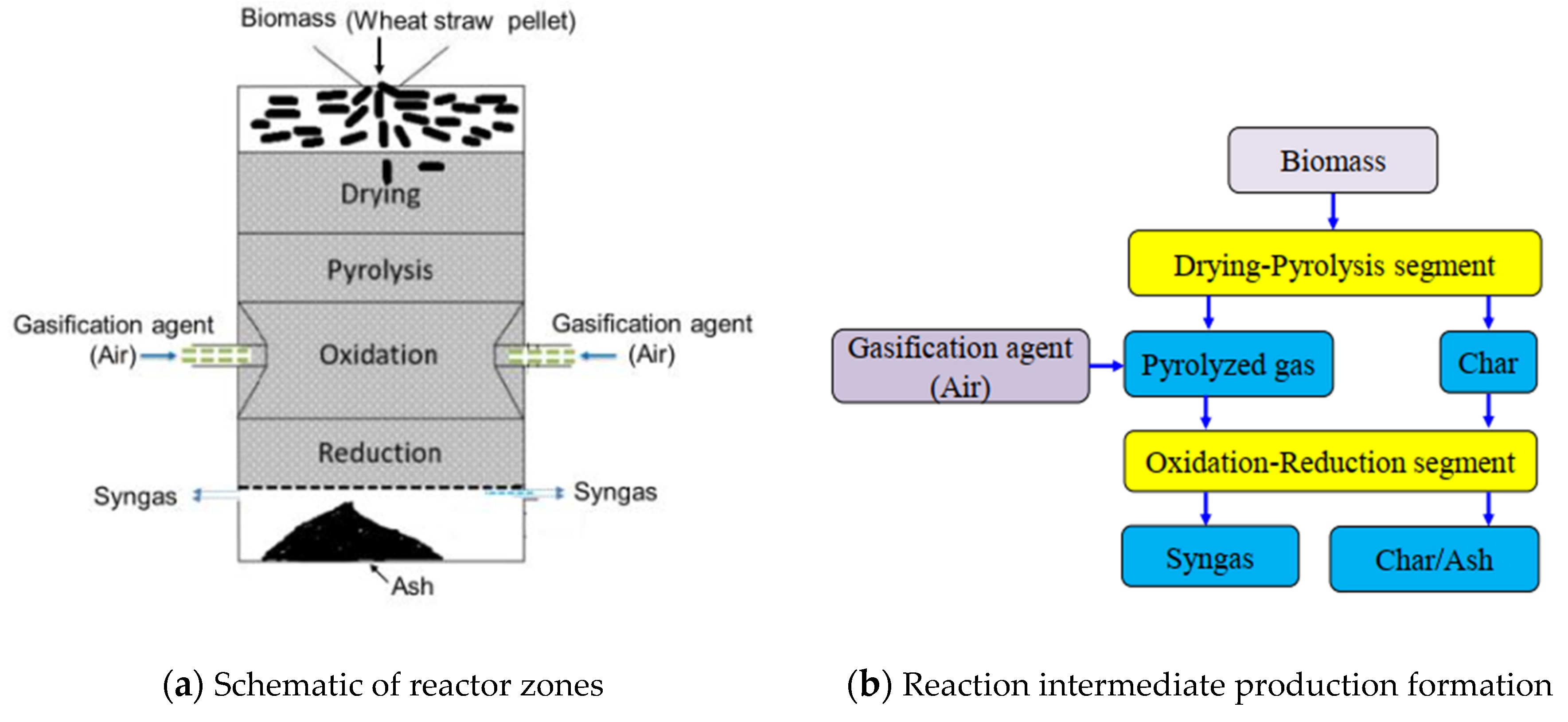
Figure 2.
Modelling scheme of solid fuel in a fixed bed downdraft gasifier [32].
Figure 2.
Modelling scheme of solid fuel in a fixed bed downdraft gasifier [32].
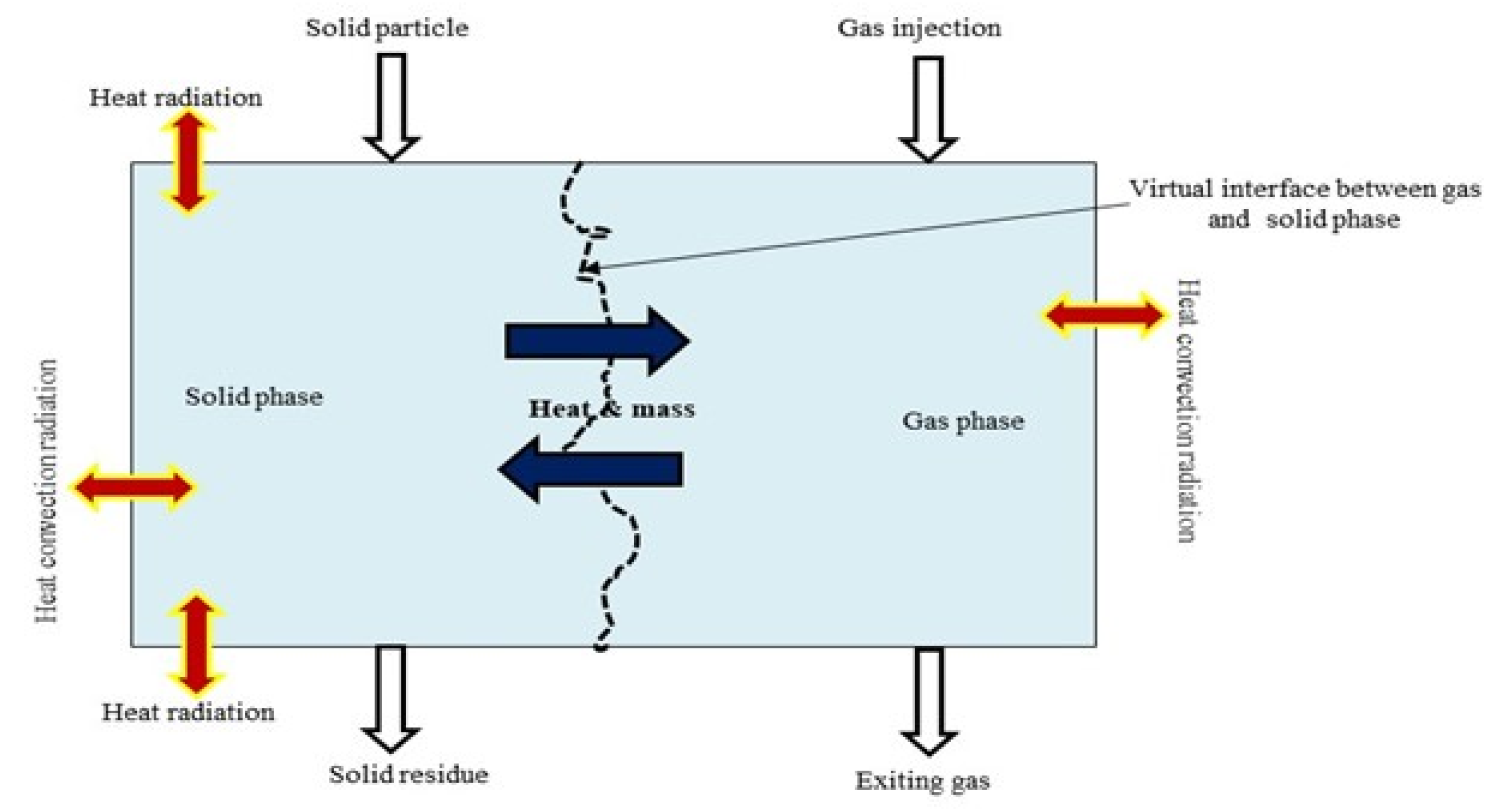
Figure 3.
Flowchart for numerical simulation of gasification using Computational Fluid Dynamics.
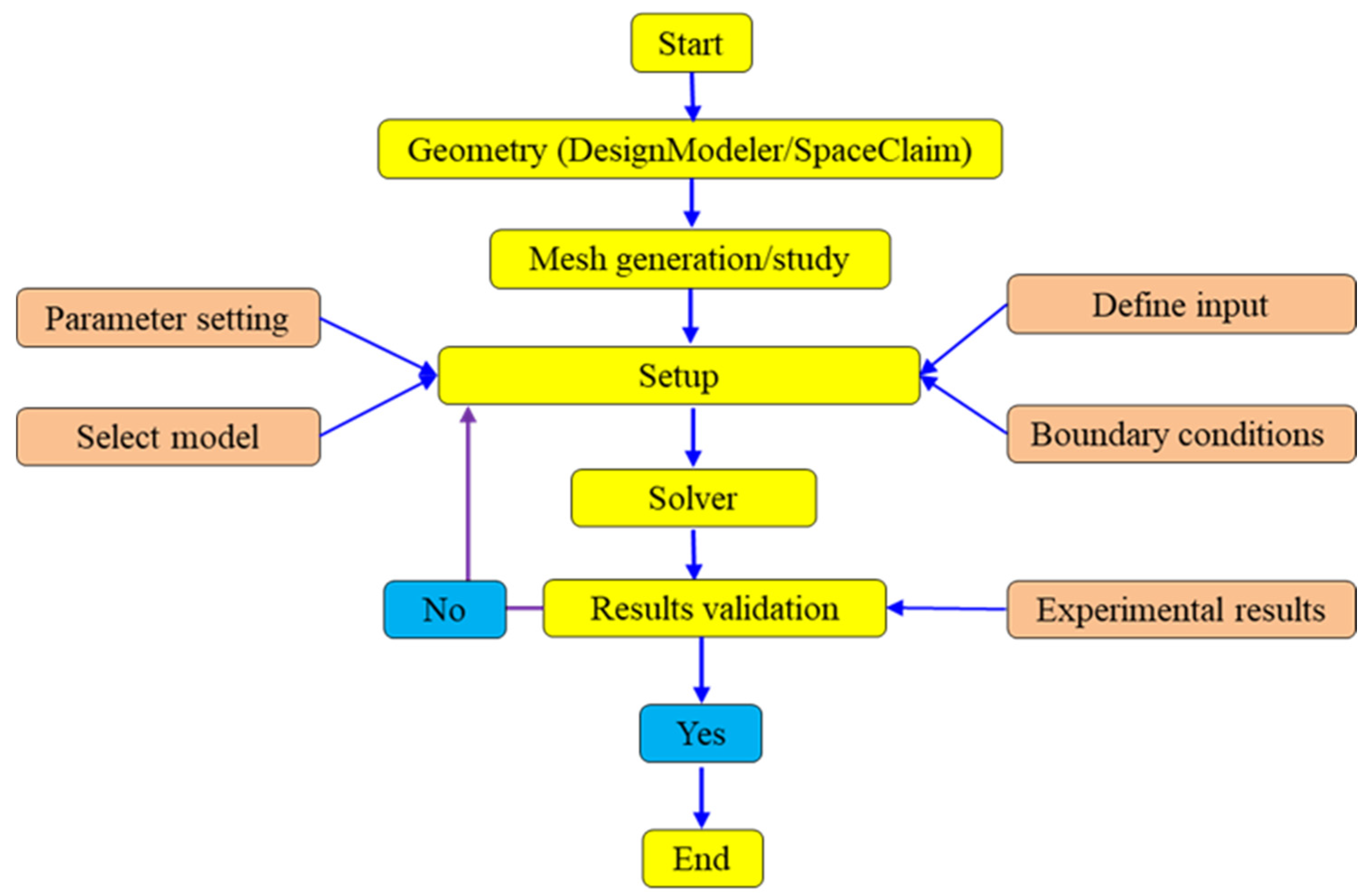
Figure 4.
Visualization of geometry and mesh details.
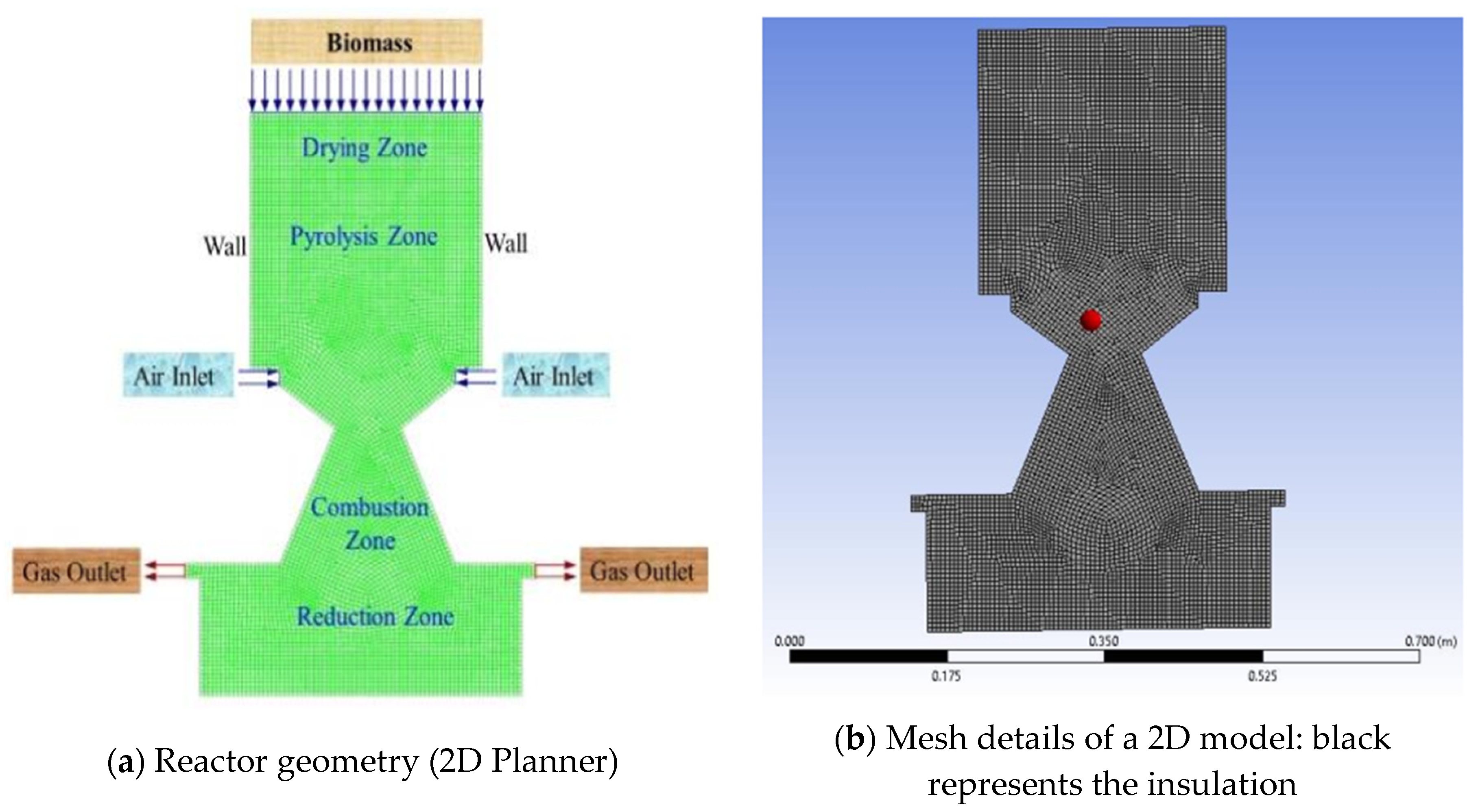
Figure 5.
Relation between velocity and vertical position of reactor regarding mesh elements.
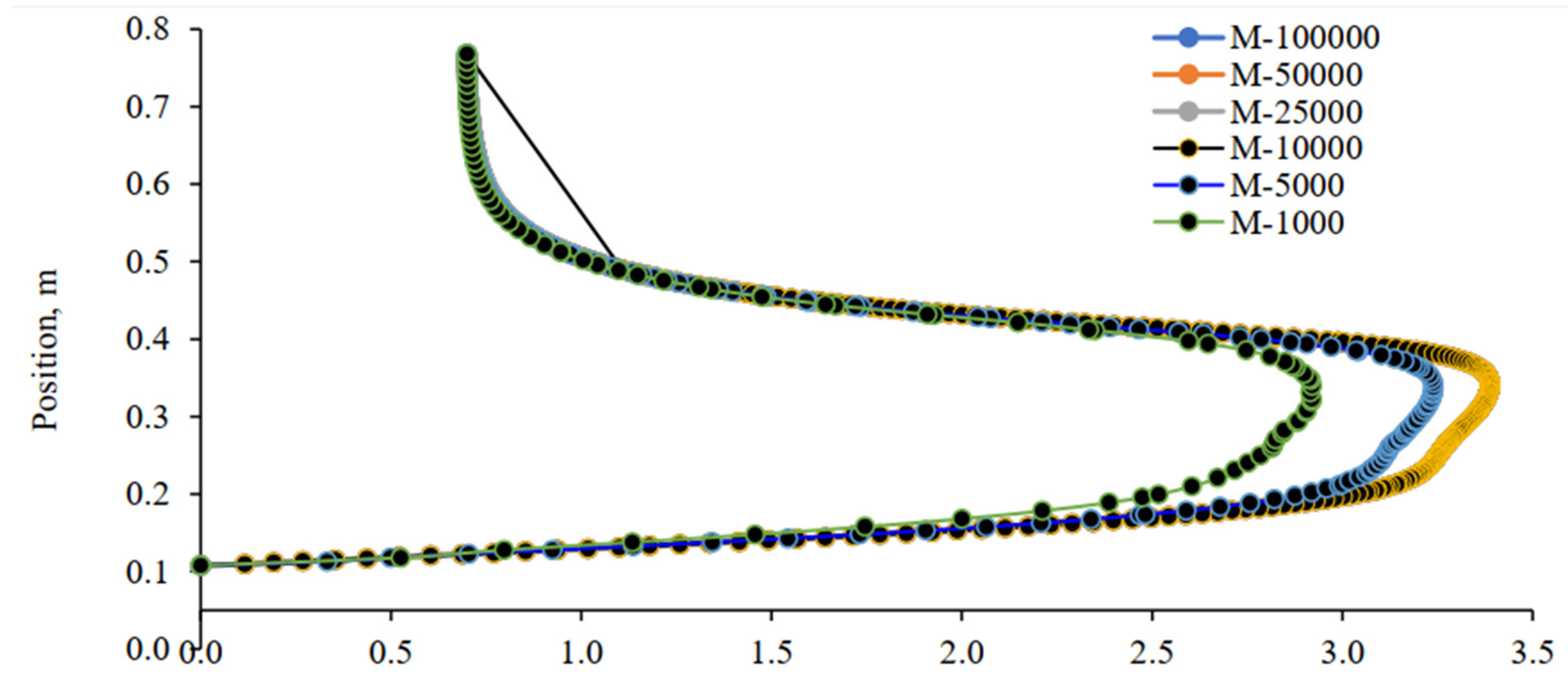
Figure 6.
Velocity comparison between the grid cells.
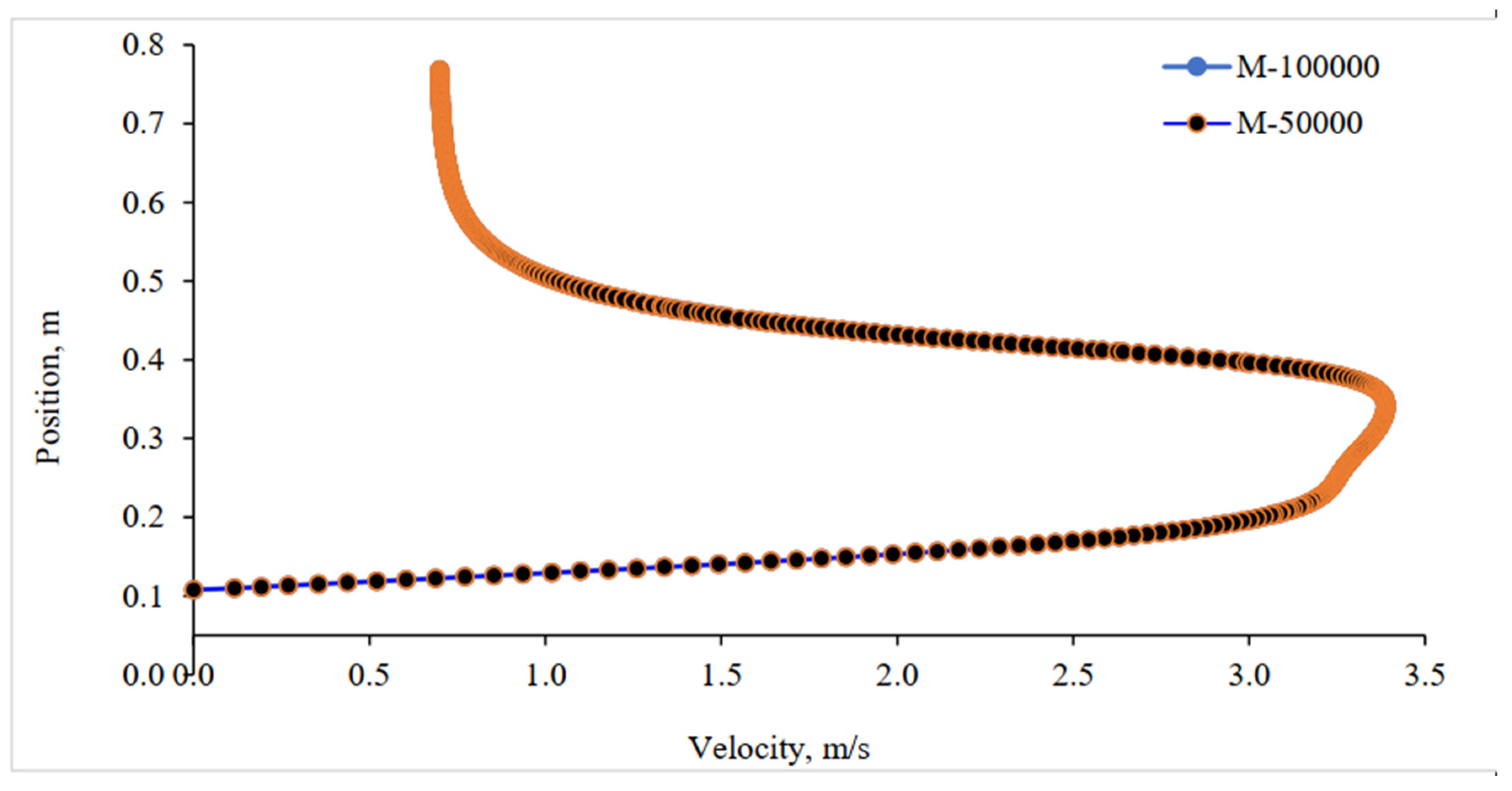
Figure 7.
Gasification experimental results.
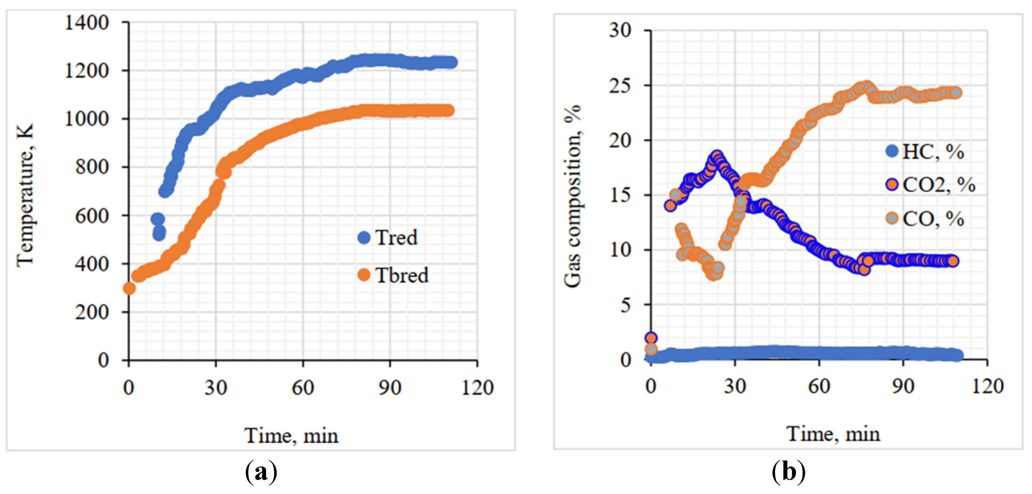
Figure 8.
Iso-surface representing the temperature in the CFD model results for gasification.
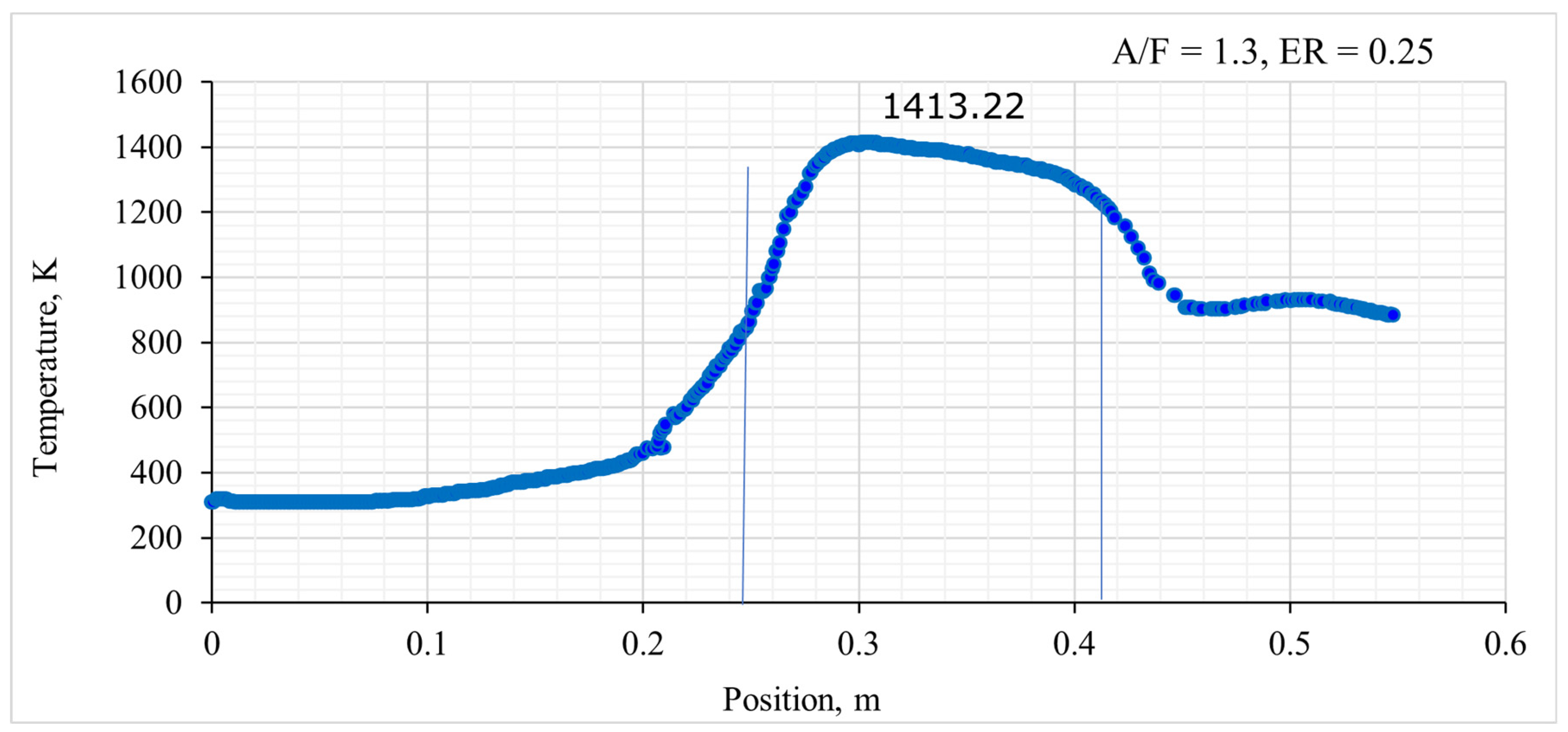
Figure 9.
Model interpretation of velocity contour.
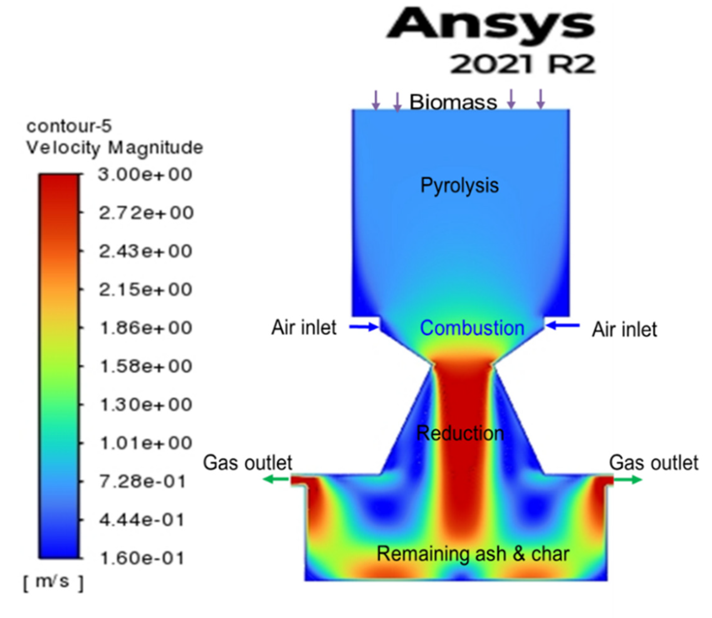
Figure 10.
Temperature profile: (a) Contour and (b) Centreline.
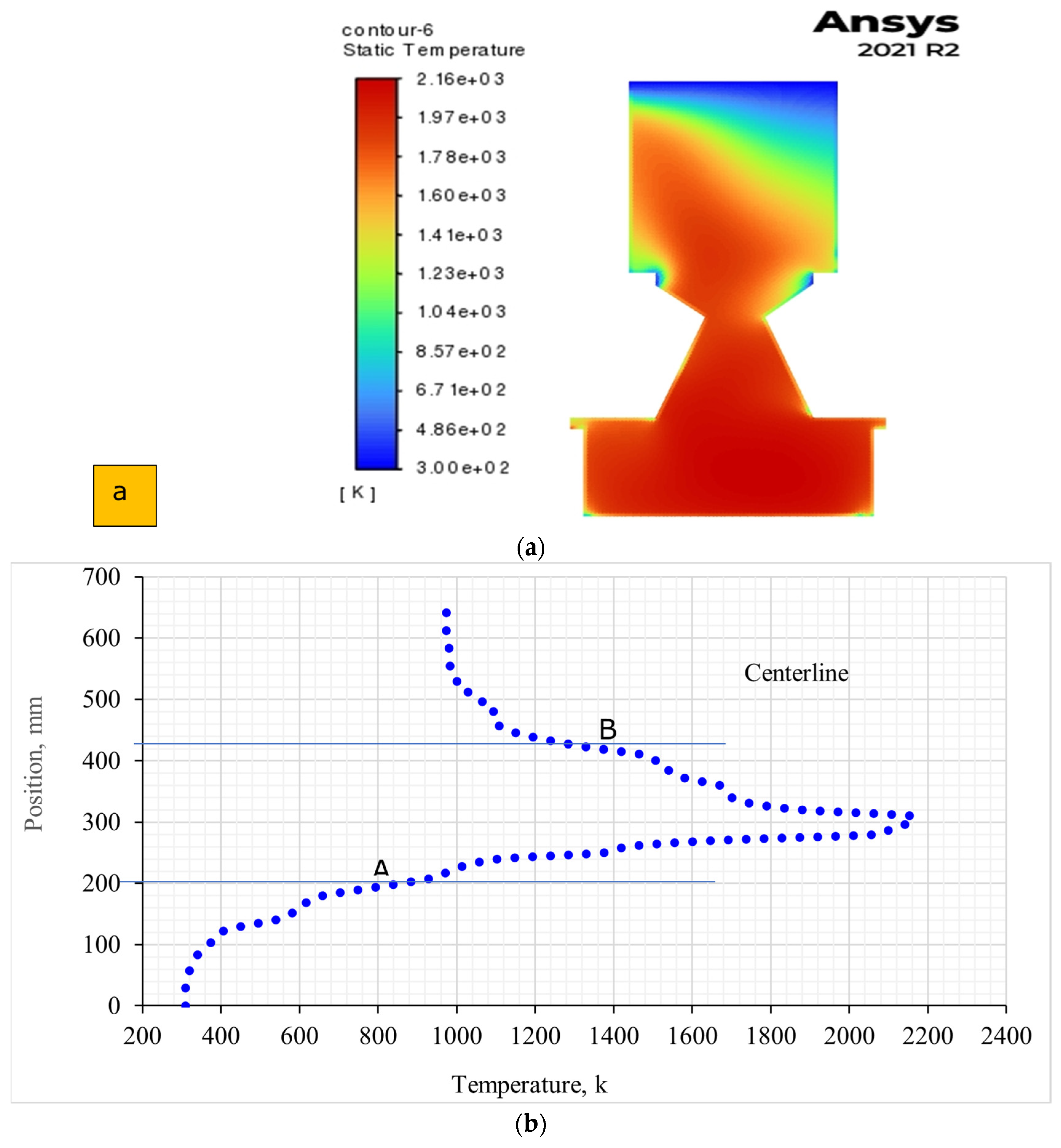
Figure 11.
Density profile: (a) Contour and (b) Centreline.
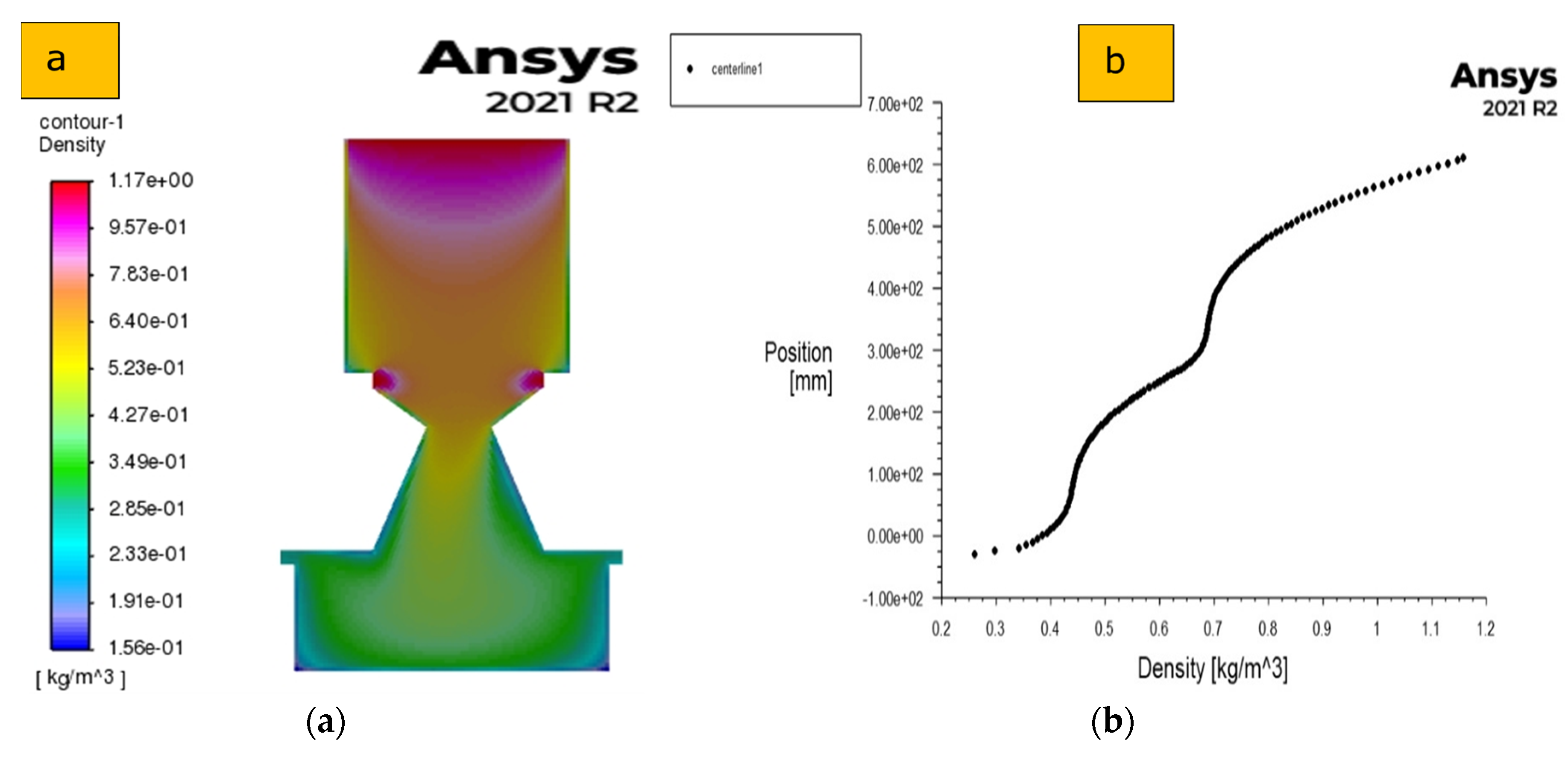
Figure 12.
Static pressure profile: (a) Contour and (b) Centreline.
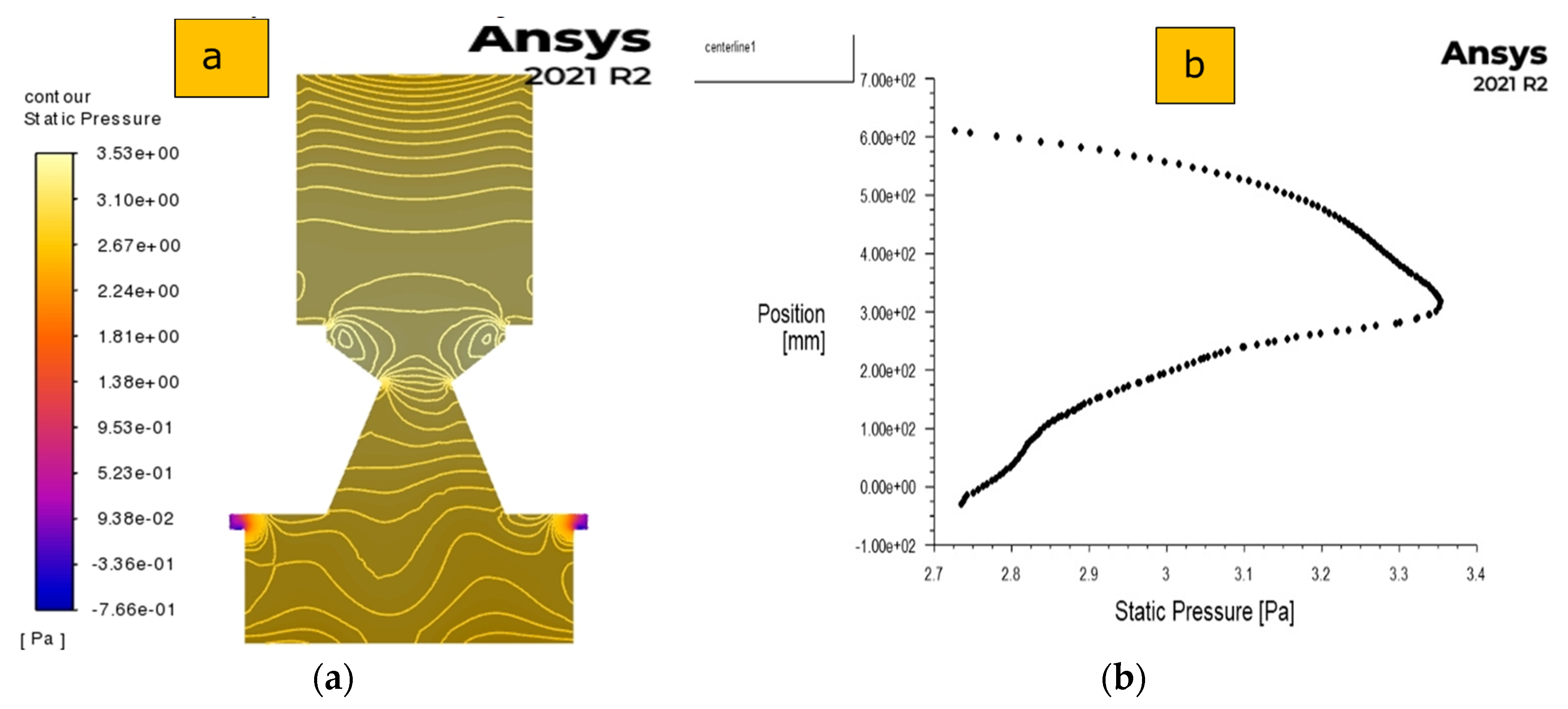
Figure 13.
Gas species contour: (a) CO2 and (b) O2 mole fraction.
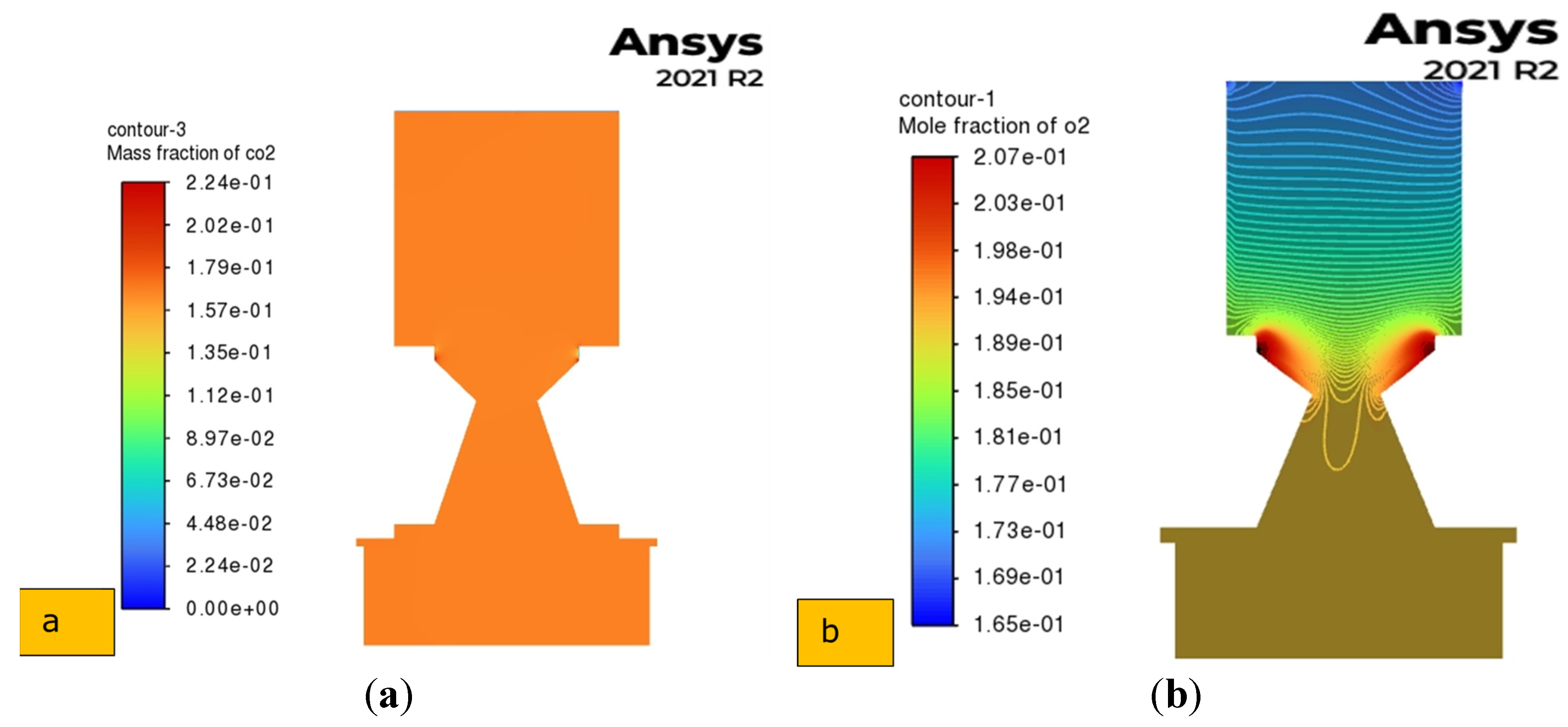
Figure 14.
Gas species contour: (a) H2O and (b) N2 mole fraction.
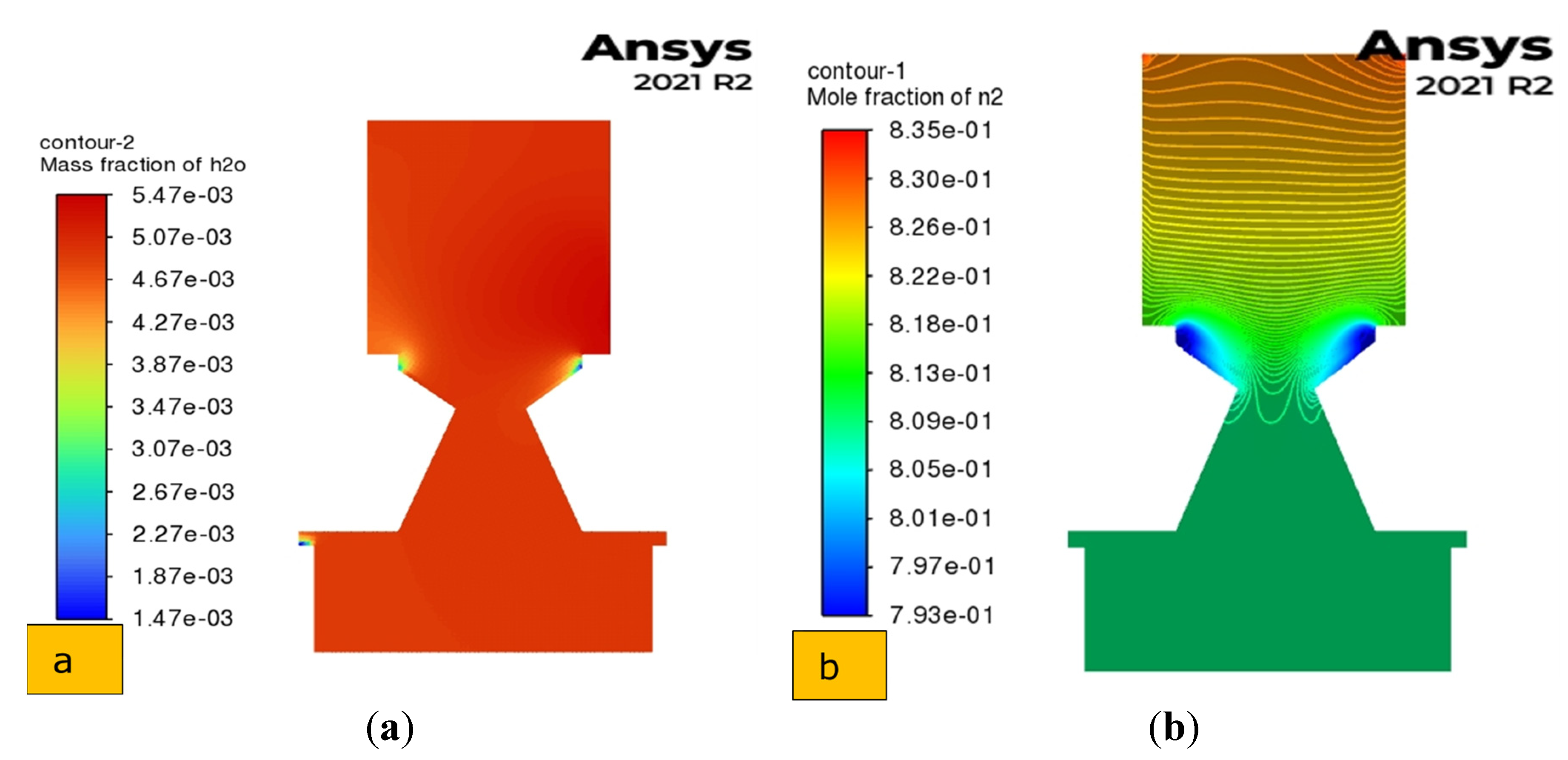
Figure 15.
Gas composition at different equivalence ratios.
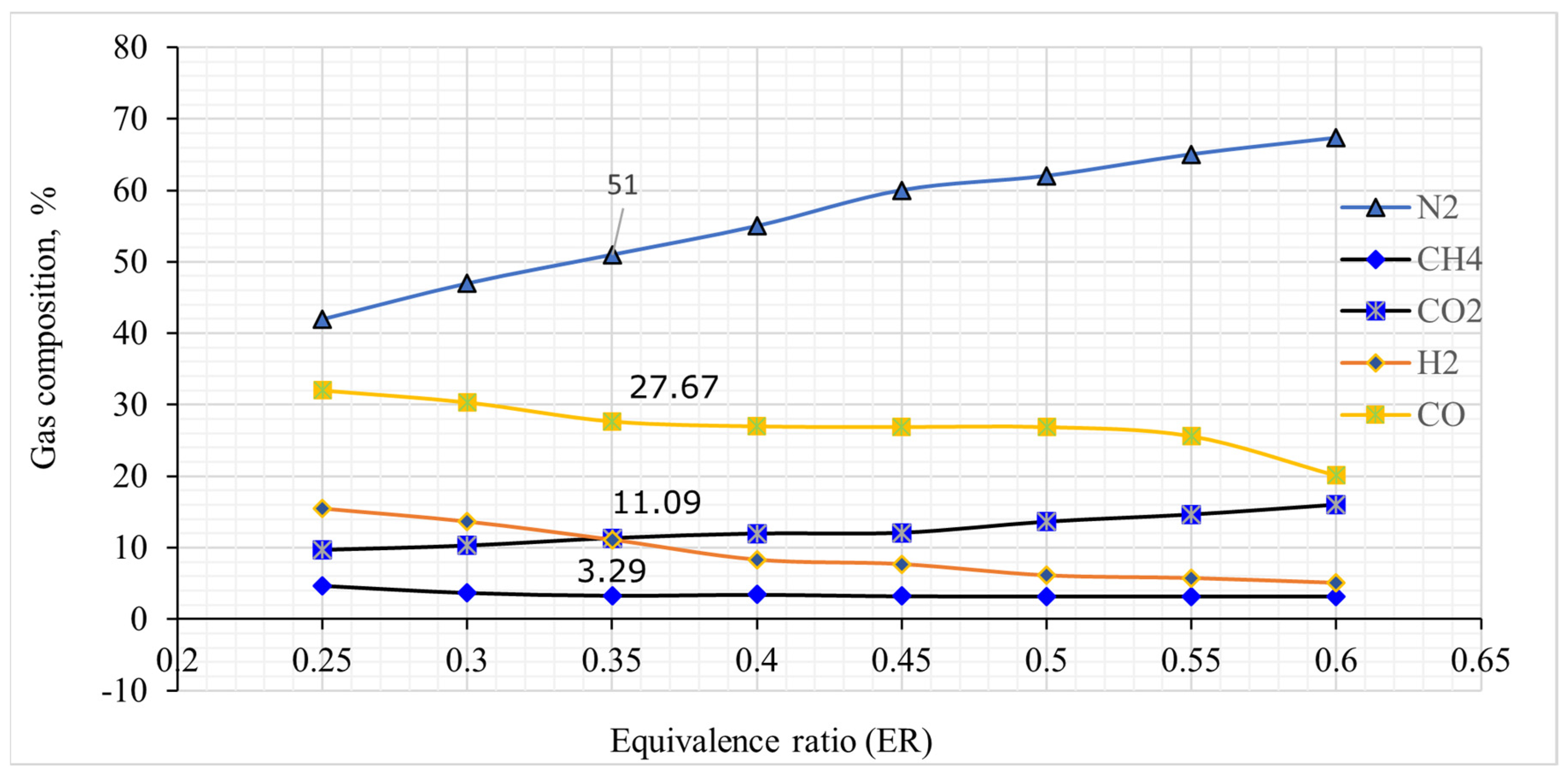
Figure 16.
Effect of temperature on gas species.
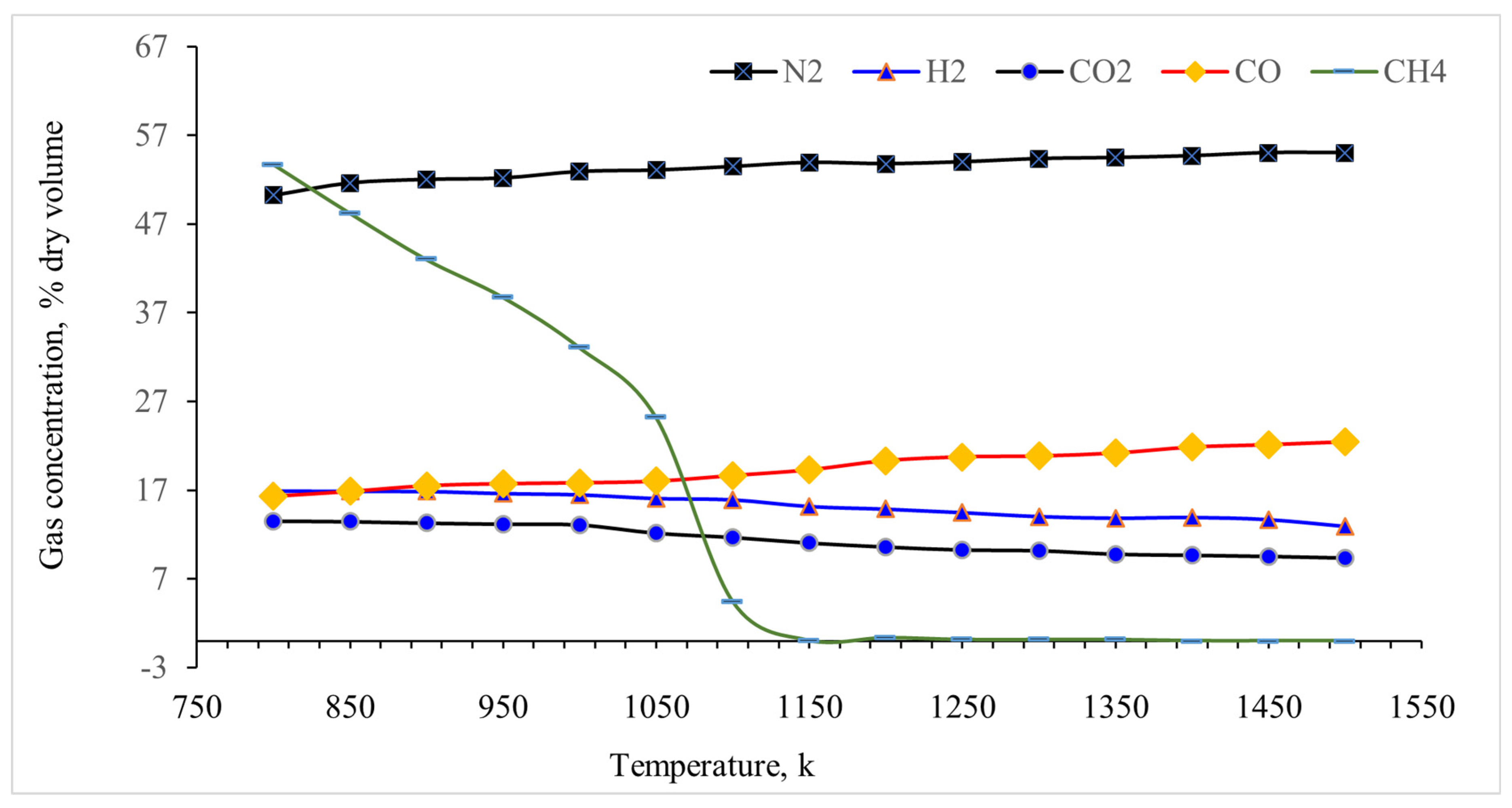
Table 1.
Biomass feedstock physiochemical characteristics.
| Pellet features | Value | |
|---|---|---|
| Proximate analysis (wt % as received, db) |
Moisture | 3.50 |
| Volatile matters | 44.51 | |
| Fixed carbon | 36.99 | |
| Ash | 15.00 | |
| Calorific value, HHV (MJ/kg) | 19.06 | |
| Ultimate analysis (wt % as received, db) |
Carbon | 45.97 |
| Hydrogen | 5.22 | |
| Nitrogen | 0.72 | |
| Sulphur | 0.21 | |
| Oxygen (by difference) | 47.88 | |
| Density | Apparent density (kg/m3) | 817.71 |
| Bulk density (kg/m3) | 427.45 | |
| Thermokinetic properties* | In combustion | |
| Activation of energy, (kJ/mol) | 418.935 | |
| Pre-exponential factor, (1/sec) | 1.76E+16 | |
| In pyrolysis | ||
| Activation of energy, (kJ/mol) | 132.868 | |
| Pre-exponential factor, (1/sec) | 2.4E+4 | |
Note; * = devolatilisation phase and heating rate 20 °C/min.
Table 2.
Representation of the model, including air, biomass, and reactor, during the gasification process.
Table 2.
Representation of the model, including air, biomass, and reactor, during the gasification process.
| Components | Computational model |
|---|---|
| Biomass |
|
| Air |
|
| Gasification |
|
Table 4.
Boundary and operating conditions of the biomass CFD model to ensure accurate simulations.
| Parameter | References | |
|---|---|---|
| Gasification agent (air) | Air flow rate: 54 kg/hr (37.87 Nm3/hr) | - |
| Air velocity: 3.2 ~7.2 m/s (average 5.2) | [1] | |
| Air fuel ratio: 6:1 v/m | [38] | |
| Air inlet temperature: 300K | [1] | |
| Pressure | Gasification pressure: 1 atm = 101325 pascal | [6] |
| Outlet gauge pressure: 0 | [30] | |
| Pressure outlet: 249 pascals (min) and 747 pascals (max) | - | |
| Biomass | Input: Biomass (WSP) inject (Gravity feed) | - |
| Gravitational acceleration: - 9.8 m/sec2 | - | |
| Biomass inlet temperature: 300°K | [2] | |
| Biomass flow rate: 9 kg/hr | [1] | |
| Biomass moisture content: 3.5% | - | |
| Temperature | Temperature-Atmospheric condition: 300K | [30] |
| Operating temperature: 300 ~ 2500K | - | |
| Reactor wall | Motion: stationary | [30] |
| Wall shear condition: No slip | ||
| Wall roughness: standard | ||
| Inlet species mass fraction of O2: 0.23 | [30] | |
| Inlet velocity magnitude: 0.056 m/sec | - | |
| Wall (interior and exterior walls): Stainless steel | - | |
| Wall thickness: 3 mm | - | |
| Others | Equivalence ratio: 0.2 ~ 0.6 | [24] |
| Turbulence intensity: 5% | [30] | |
| Particle-specific heat: 2.5 kJ/kgK | [30] | |
| Particle size in the discrete phase: 0.1 mm | [2] | |
| Uniform porosity: 0.5 | [54] | |
| For simulation time setup: 10 sec | [30] | |
| Model run: 0 to 7200 sec | ||
Table 5.
Summary of the model used for the gasification of wheat straw pellets.
|
Conditions/Assumptions |
|
|
|
P1: Radiation reflection at the surface is isotropic |
|
-intermittency: Include the effect of share stress transport, kinetic and its dissipation rate and the change in velocity |
|
Nonpremix combustion-non-adiabatic |
|
Euler-Lagrange (discrete phase)Particle devolatilisation model: Single kinetic rate Particle combustion: Kinetic/diffusion-limited rate |
Table 6.
Particulars of the biomass CFD model solver.
| Variable | Discretisation Scheme | Information |
|---|---|---|
| Pressure staggering option | PRESTO! | Pressure-based Navier-Stokes solution algorithm (the default) |
| Pressure velocity coupling | SIMPLE | Governing equation |
| Gradient option | Least Squares Cell-based | - |
| Pressure | Second Order Upwind | Spatial discretisation |
| Momentum | Second Order Upwind | Spatial discretisation |
| Turbulent Kinetic Energy | Second Order Upwind | Spatial discretisation |
| Turbulent Dissipation Rate | Second Order Upwind | Spatial discretisation |
| Energy | Second Order Upwind | Spatial discretisation |
| Mean mixture fraction | First Order Upwind | Spatial discretisation |
| Mixture fraction variance | Second Order Upwind | Spatial discretisation |
| Soot | Second Order Upwind | Spatial discretisation |
| Others | First order Upwind | - |
| Discrete ordinates | Second Order Upwind | Spatial discretisation |
| Formulation | Implicit | - |
| Velocity formulation | Absolute | default setting |
| Porous formulation | Superficial velocity | - |
| Initialisation | Hybrid | - |
Table 3.
Solid particle surface reactions [53].
Table 3.
Solid particle surface reactions [53].
| Gas phase reaction | Solid particle surface reactions | ||
|---|---|---|---|
| Reaction | Reaction order | Reaction | Reaction order |
| Volatile decomposition | Char decomposition | ||
| CO Combustion: | |||
| H2 Combustion: O | |||
| Water-gas shift: | |||
Table 7.
Simulated mesh cells, and mesh statistics of developed model.
| Particulers | Value | |
|---|---|---|
| Mesh element size (average) | : | 1 mm |
| No of nodes | : | 172677 |
| No of elements | : | 171558 with a rectangular shape |
| Minimum orthogonal quality | : | 0.38916 |
| Maximum aspect ratio | : | 5.27929. |
Table 8.
Result comparison: CFD gasification model and gasification.
| Particulars | Results | ||
|---|---|---|---|
| Model | Experiments | ||
| Temperature (k) | Combustion (Upper concentric at x = 0.25 to 0.3 m) |
900~1413 | 1250 |
| Reduction (Bottom reduction at x = 0.425 m) |
1100 | 1080 | |
| Gas species (% v/v) |
CO2 | 9.99 | 9.4 |
| CO | 21.60 | 23.3 | |
| CH4 | 0.13 | 0.051 | |
| H2 | 16.81 | N/A | |
Table 9.
CFD simulation temperature at air-fuel ratio 6:1 and ER =0.35.
| Zone | Temperature range, k |
|---|---|
| Drying and pyrolysis | 300~856 |
| Combustion | 856~1356 (Max temp. 2160) |
| Reduction | 1356~974 |
Disclaimer/Publisher’s Note: The statements, opinions and data contained in all publications are solely those of the individual author(s) and contributor(s) and not of MDPI and/or the editor(s). MDPI and/or the editor(s) disclaim responsibility for any injury to people or property resulting from any ideas, methods, instructions or products referred to in the content. |
© 2024 by the authors. Licensee MDPI, Basel, Switzerland. This article is an open access article distributed under the terms and conditions of the Creative Commons Attribution (CC BY) license (http://creativecommons.org/licenses/by/4.0/).
Copyright: This open access article is published under a Creative Commons CC BY 4.0 license, which permit the free download, distribution, and reuse, provided that the author and preprint are cited in any reuse.


