A Modified Aeromagnetic Compensation Method Robust to In-Cabin OBE Interferences

Yuxin Liu; Wen Li; Dongyan Wei; Ge Shen

doi:10.20944/preprints202401.1460.v1

Preprint

Technical Note

A Modified Aeromagnetic Compensation Method Robust to In-Cabin OBE Interferences

This version is not peer-reviewed.

Wen Li^*,

Wen Li^*,

This version is not peer-reviewed.

Downloads

189

Views

Comments

Submitted:

19 January 2024

Posted:

19 January 2024

You are already at the latest version

Abstract

Aeromagnetic compensation plays a vital role in geomagnetic navigation and has received considerable attention throughout last few decades. Classical aeromagnetic compensation methods based on the Tolles–Lawson (T-L) model are mainly aimed at permanent, induced, and eddy-current magnetic interferences of aircraft platform, which ignores other stray magnetic field interference on the platform including the interferences caused by on-board electronic (OBE) systems. In order to cooperate with TL model, magnetometers are usually required to be installed on the extension rod outside the cabin, which is widely applied to geophysical magnetic survey. In order to ensure safety and reduce the cost of platform modification in geomagnetic navigation, it’s necessary to place magnetometers inside the cabin. It also further exacerbates the magnetic interferences and improves the difficulty of magnetic compensation. In this paper, a modified aeromagnetic compensation method is proposed, and the in-cabin OBE interferences are respectively modelled to be proportional to the currents and their temporal variations of different electronic devices. To ensure that modified model adapts to strong OBE interference in the cabin, a cut-off frequency determination method based on curvature calculation and a feature selection method based on correlation calculation are proposed. The cut-off frequency determination method helps to select passband filter which suitable for in-cabin OBE interference. The feature selection method can help to effectively select current and voltage inputs for modified model. In addition, principal component analysis (PCA) is adopted to reduce multicollinearity which is intensified by the extension of OBE interferences in coefficient-estimating. Experiments on public dataset are conducted to illustrate the effectiveness of the proposed method, and the best compensation result achieved 1.71nT of root mean square error (RMSE).

Keywords:

aeromagnetic compensation

;

magnetic survey

;

magnetic interference

;

on-board electronic systems

;

geomagnetic navigation

Subject:

Environmental and Earth Sciences - Remote Sensing

1. Introduction

The geomagnetic navigation has the benefits of being passive, globally available at any time and in any weather, and not reliant on satellites or other external communications, which has shown promise as a viable alternative to the Global Positioning System (GPS) [1]. The basic principle of geomagnetic navigation is the matching of the real-time magnetic field data collected by the magnetometers with ready-made magnetic maps of the earth. However, the desired magnetic signal for geomagnetic navigation will be disrupted by the aircraft platform. Besides, the magnetometers are required to be placed inside the cabin in consideration of safety and practicality. Therefore, elimination of magnetic interferences inside the cabin is always a challenging problem in geomagnetic navigation [2,3].

For decades, much work has been carried out for aeromagnetic compensation. The classical aeromagnetic compensation model was proposed by Tolles and Lawson in the 1950's [4], which identifies three types of magnetic interferences as permanent, induced, and eddy-current fields. Then the classical 21st-order linear model, Tolles–Lawson (T-L) model, which models the magnetic interference as a function of the aircraft orientation with respect to the geomagnetic field was established. And a lot of related research have been conducted including modelling evaluation and error analysis [5,6,7,8,9,10]. The estimated coefficients of the Tolles–Lawson model are used to calculate and remove the magnetic interference caused by aircraft. However, the incomplete sampling and the multicolinearity of the system of linear equations always constrain the accuracy of the coefficients. Therefore, much research on the improvement of parameter estimation method due to multicollinearity or other factors are conducted [11,12,13,14,15,16,17]. In addition, there are also researches on the extension and modification of the model due to other interference sources, such as the influences of geomagnetic gradient, on-board electronic (OBE) systems [18,19,20,21,22,23,24], etc.

When the magnetometer is installed outside the cabin, the existing aeromagnetic compensation methods based on TL model can achieve good compensation effects. However, the in-cabin installation of magnetometers will result in more severe OBE interferences, which cannot be effectively eliminated yet. According to the Biot-Savart Law, the OBE interferences are modeled as a component proportional to the electric current [20]. Another compensation algorithm could remove any ON/OFF effects in the magnetic data while recovering the original data to its normal trend [21]. In addition, a real-time dynamic compensation method is proposed to eliminate the OBE interferences, and designs two compensation modes for constant current draw and slow-varying current [22]. In terms of the interference of specific electronic device, an improved aeromagnetic compensation method is proposed and the OBE interferences are modelled to be proportional to the currents of strobe and beacon lights [23]. The above researches provide potential solutions for eliminating the OBE interferences on the external mounting magnetometers, whose vast majority of applications is geophysical magnetic surveying. Aimed at the in-cabin aeromagnetic data for navigation, a neural network-based model is proposed [24], but it lacks generalization ability on other test set.

It's clear that the OBE interferences are non-ignorable for in-cabin geomagnetic compensation, but there is no systematic solution so far. In contrast to the interferences of external mounting magnetometers, the process of in-cabin OBE interferences faces more severe impact of more interference sources. The challenges include model extension for more interference terms, determination of the optimal cutoff frequency for bandpass filters, the selection of effective interference sources, reduction of multicollinearity’s impact and so on. These challenges make existing compensation methods for OBE interferences can’t be applied to in-cabin magnetic compensation directly.

The contribution of this paper is a modified compensation method for in-cabin interferences caused by on-board electronic systems. The direct impact of OBE current and the indirect impact of the induced and eddy-current effect caused by its variations are taken into consideration. The OBE interferences are modelled to be proportional to the currents and their temporal variations, which are merged to the classical aeromagnetic compensation model finally. To ensure that extended model adapts to strong OBE interference in the cabin, a cut-off frequency determination method based on curvature calculation and a feature selection method based on correlation calculation are proposed. The cut-off frequency determination method helps to select passband filter which suitable for in-cabin OBE interference. The feature selection method can help to effectively select current and voltage inputs for extended model. Finally, the principal component analysis (PCA) is adopted as preprocessing step in coefficient-estimating to reduce the effect of multicollinearity caused by model extension.

The paper is organized as four sections. Section 2 introduces the modified aeromagnetic compensation method including cut-off frequency determination, feature selection and principal component analysis. Section 3 includes the experiment results on public dataset and related discussion. Section 4 is the conclusion of this research.

2. Proposed Aeromagnetic Compensation Method

2.1. Overall Method Framework

The overall method framework is shown in Figure 1. The inputs of the model include scalar magnetic field, vector magnetic field, and a series of voltage and current measurements. Firstly, the classical TL model is used for the compensation of in-cabin magnetic measurements. Then, FFT is performed on TL model compensated data, which can reflect the frequency domain distribution of TL model compensation residuals. According to FFT discrete points, curve fitting based on exponential function is performed and the maximum curvature point of the fitted curve is the optimal cutoff frequency of bandpass filtering.

After the bandpass filtering process, the correlation coefficients between electrical measurements and magnetic data are calculated, and the contribution of different electrical features can be evaluated by the softmax function. Then select useful features based on their contribution percentage.

The selected features will be used as inputs to the model. Before the calculation of model coefficients, PCA is adopted to reduce multicollinearity caused by model extension. Finally, the model coefficients are calculated using the least squares method and the magnetic interference of the aircraft can be calculated. After the compensation process, compensated data can be obtained, and clean magnetic field signals can be used for geomagnetic navigation.

2.2. The Classical Aeromagnetic Compensation Model

In classical aeromagnetic compensation theory, the magnetometer measurement

{\vec{B}}_{t}

is the superposition of the geomagnetic field

{\vec{B}}_{e}

and the magnetic interference

{\vec{B}}_{a}

caused by the aircraft.

{\vec{B}}_{t} = {\vec{B}}_{e} + {\vec{B}}_{a}

(1)

The magnitude of

{\vec{B}}_{e}

is the desired signal for geomagnetic navigation. According to the Tolles–Lawson model, the magnetic interference caused by the aircraft is comprised of permanent, induced, and eddy current magnetic interferences.

{\vec{B}}_{a} = {\vec{B}}_{p e r m} + {\vec{B}}_{i n d u} + {\vec{B}}_{e d d y}

(2)

The permanent magnetic interference terms stem from the nearly permanent magnetization of various ferromagnetic aircraft components. It will not change significantly in a short period of time, and it is not related to the excitation magnetic source, which is usually considered as geomagnetic field. The induced magnetic interference stems from the changeable magnetization of magnetically susceptible aircraft components. The induced magnetization will be affected by the relative orientation of the aircraft and the excitation magnetic source. The eddy current terms stem from the electrical current loops caused by the time-varying magnetic field relative to the aircraft interacting with electrically conductive aircraft components. The eddy currents depend on the time rate of variation of the excitation magnetic field flux through these aircraft components.

When the magnetometer is installed outside the cabin, the excitation source is considered to be geomagnetic field since the magnitude of other stray magnetic interference is far smaller. Based on this assumption, the magnitude of magnetic measurement can be approximated by

|{\vec{B}}_{t}| \approx |{\vec{B}}_{e}| + \frac{{\vec{B}}_{a} \cdot {\vec{B}}_{t}}{|{\vec{B}}_{t}|}

(3)

where

\frac{{\vec{B}}_{a} \cdot {\vec{B}}_{t}}{|{\vec{B}}_{t}|}

represent the effect of the aircraft interference field projected onto the total magnetic field, which uses the total field direction cosines

\vec{u} = \frac{{\vec{B}}_{t}}{|{\vec{B}}_{t}|} = {[\begin{matrix} \cos α & \cos β & \cos γ \end{matrix}]}^{T} = \vec{i} \cos α + \vec{j} \cos β + \vec{k} \cos γ

(4)

where

\vec{i}

\vec{j}

\vec{k}

represent the three axes of the aircraft coordinate system, and

α

β

γ

represent the angle between the geomagnetic vector measurement and the three axes of the aircraft coordinate system. Then the standard Tolles-Lawson model can be summarized as

|{\vec{B}}_{t}| \approx |{\vec{B}}_{e}| + ({\vec{u}}^{T} [\begin{matrix} x_{1} \\ x_{2} \\ x_{3} \end{matrix}] + |{\vec{B}}_{t}| {\vec{u}}^{T} [\begin{matrix} x_{4} & x_{5} & x_{6} \\ \cdot & x_{7} & x_{8} \\ \cdot & \cdot & x_{9} \end{matrix}] \vec{u} + |{\vec{B}}_{t}| {\vec{u}}^{T} [\begin{matrix} x_{10} & x_{11} & x_{12} \\ x_{13} & x_{14} & x_{15} \\ x_{16} & x_{17} & x_{18} \end{matrix}] \dot{\vec{u}})

(5)

The above equation can be rewritten into matrix form as

|{\vec{B}}_{t}| - |{\vec{B}}_{e}| = A \vec{x}

(6)

A bandpass finite impulse response filter (bpf) is applied to remove the earth magnetic field while remaining the aircraft magnetic interference field. Then the equation can be rewritten as

b p f (|{\vec{B}}_{t}|) = b p f (A) \vec{x}

(7)

In existing research, the cutoff frequency range of the bandpass filter is 0.1-0.9 Hz[24]. Data for model coefficients calculation comes from a calibration flight at a high altitude, which contains a specific set of roll, pitch, and yaw aircraft maneuvers. Then the Tolles-Lawson coefficient vector can be calculated by linear least squares regression.

\vec{x} = {(A_{f}^{T} A_{f})}^{- 1} A_{f}^{T} \vec{y}

(8)

where

\vec{y} = b p f (|{\vec{B}}_{t}|)

A_{f} = b p f (A)

. Finally, the earth magnetic field for navigation can be calculated as

|{\vec{B}}_{e}| = |{\vec{B}}_{t}| - A \vec{x}

(9)

2.3. The Modified Model for OBE Interferences

According to Biot-Savart's Law, the OBE interferences are caused by the current flowing through on-board electronic systems, so it’s reasonable to evaluate the interference magnetic fields by monitoring the current flowing. Moreover, triaxial components of OBE interferences should be proportional to the current flowing measurements, which can be calculated as follows

{\vec{B}}_{I_k} = I_{k} (a_{1} \vec{i} + a_{2} \vec{j} + a_{3} \vec{k})

(10)

where

I_{k}

represents the electric current observation of the k-th electronic device in the cabin.

a_{1}

a_{2}

a_{3}

represent the different influence of airborne electronic systems on the magnetic field in the three axes’ direction of the magnetometer.

In order to obtain the magnitude of OBE interferences, it should also be projected onto the direction of the total magnetic field as equation (3)

|{\vec{B}}_{I_k}| = \frac{{\vec{B}}_{I_k} \cdot {\vec{B}}_{t}}{|{\vec{B}}_{t}|} = a_{1} I_{k} \cos α + a_{2} I_{k} \cos β + a_{3} I_{k} \cos γ

(11)

In T-L model, the excitation magnetic sources of the induced and eddy current magnetic field are considered to be the geomagnetic field. When the magnetometer is installed inside the cabin, the close installation distance of electrical devices makes the scale of OBE interference’s variation have comparability with the variation of geomagnetic field. It means that OBE interferences should be considered to be a part of the excitation source. The induced magnetic field caused by OBE interferences can be calculated as

\begin{array}{l} {\vec{B}}_{i n d u_I_k} = a_{1} I_{k} (σ_{11} \vec{i} + σ_{12} \vec{j} + σ_{13} \vec{k}) \\ + a_{2} I_{k} (σ_{21} \vec{i} + σ_{22} \vec{j} + σ_{23} \vec{k}) \\ + a_{3} I_{k} (σ_{31} \vec{i} + σ_{32} \vec{j} + σ_{33} \vec{k}) \end{array}

(12)

where

σ_{i j}, i, j = 1, 2, 3

represent the coefficient of induced magnetic intensity caused by OBE interferences.

The eddy current magnetic field caused by the temporal variation of OBE interferences can be calculated as

\begin{array}{l} {\vec{B}}_{e d d y_I_k} = a_{1} I_{k}' (μ_{11} \vec{i} + μ_{12} \vec{j} + μ_{13} \vec{k}) \\ + a_{2} I_{k}' (μ_{21} \vec{i} + μ_{22} \vec{j} + μ_{23} \vec{k}) \\ + a_{3} I_{k}' (μ_{31} \vec{i} + μ_{32} \vec{j} + μ_{33} \vec{k}) \end{array}

(13)

where

I'

represent the temporal variation of the current measurement, and

μ_{i j}, i, j = 1, 2, 3

represent the coefficient of eddy current magnetic intensity caused by OBE interferences.

Similarly, the induced and eddy current magnetic field caused by OBE interferences should also be projected onto the direction of the ambient magnetic field, and their total magnitude can be calculated as follows:

\begin{array}{l} |{\vec{B}}_{O B E_k}| = \frac{({\vec{B}}_{I_k} + {\vec{B}}_{I_i n d u_k} + {\vec{B}}_{I_e d d y_k}) \cdot {\vec{B}}_{t}}{|{\vec{B}}_{t}|} \\ = I_{k} (c_{1} \cos α + c_{2} \cos β + c_{3} \cos γ) + I_{k}' (c_{4} \cos α + c_{5} \cos β + c_{6} \cos γ) \end{array}

(14)

According to Ohm's law, the current in a wire is usually proportional to the voltage. During actual data processing, the voltage measurements can also be used to describe OBE interference characteristics, which take the place of current measurement in above equation. And the above equation can be rewritten into matrix form:

|{\vec{B}}_{O B E_k}| = I_{k} {\vec{c}}_{k}

(15)

The magnetic compensation model become

{\vec{B}}_{t} = {\vec{B}}_{e} + {\vec{B}}_{a} + \sum_{k} {\vec{B}}_{O B E_k}

(16)

\sum_{k} {\vec{B}}_{O B E_k}

represent the OBE interferences caused by k electronic equipment which have impact on magnetic measurements. In order to facilitate parameter calculation, the attitude information matrix and the current information matrix can be merged. Then the extended compensation model can be summarized as

|{\vec{B}}_{t}| - |{\vec{B}}_{e}| = A \vec{x} + \sum_{k} I_{k} {\vec{c}}_{k} = H {\vec{x}}_{t o t a l}

(17)

The bandpass finite impulse response filter should also be applied to the above equation:

\vec{y} = H_{f} {\vec{x}}_{t o t a l}

(18)

where

\vec{y} = b p f (|{\vec{B}}_{t}|)

H_{f} = b p f (H)

2.4. Cutoff Frequency Determination and Feature Selection

Due to the difference of between the internal and external environments of the cabin, the empirical filtering cutoff frequency may no longer be applicable to in-cabin magnetic compensation. Therefore, it is necessary to use appropriate methods to reselect the filtering cutoff frequency of the bandpass filter. The practice of manually selecting low cutoff frequencies from the spectrogram through fast Fourier transform has strong subjectivity. The spectral shape of the geomagnetic field signal is similar to exponential function, with many burrs doped in it. Therefore, curve fitting on the spectral curve can be performed and then the optimal cutoff frequency can be determined through curvature calculation. Assuming the selected fitting curve is

y = f (x) = a_{1} \cdot e^{b_{1} \cdot x} + a_{2} \cdot e^{b_{2} \cdot x}

(19)

where

a_{1}, a_{2}, b_{1}, b_{2}

are unknown curve fitting parameters. The calculation of curvature for discrete points is as follows

k = \frac{|y''|}{{(1 + y'^{2})}^{\frac{3}{2}}}

(20)

where

y'

and

y''

are the first and second derivatives of the curve fitting function, respectively. The first and second derivatives of discrete points are calculated as follows

y' (i) = \frac{y (i + 1) - y (i)}{x (i + 1) - x (i)}

(21)

y'' (i) = \frac{y' (i + 1) - y' (i)}{x (i + 1) - x (i)}

(22)

In addition, not every electronic device will have a significant impact on magnetic measurement. The existing research relies on experience to select useful current observations such as strobe light and beacon lights. However, magnetometers installed inside the cabin will be influenced by more electronic devices’ interference. It’s necessary to select useful inputs from a series of current and voltage measurements. Firstly, the calculation of correlation coefficients are as follows

r = \frac{\sum_{i = 1}^{n} (m_{i} - \bar{m}) (n_{i} - \bar{n})}{\sqrt{\sum_{i = 1}^{n} {(m_{i} - \bar{m})}^{2}} \cdot \sqrt{\sum_{i = 1}^{n} {(n_{i} - \bar{n})}^{2}}}

(23)

where

m

n

represent the filtered magnetic and current/voltage measurements, respectively. And

\bar{m}

\bar{n}

represent the mean of measurements. After uniformly scaling the correlation coefficients, the contribution of each measurement can be evaluated through the softmax function as follows

c_{i} = \frac{e^{r_{i}}}{\sum_{i = 1}^{n} e^{r_{i}}}

(24)

In this way, the sum of each measurement’s contribution

c_{i}

is 1. Features with high contribution after sorting can be selected as model inputs.

2.5. Estimation of Model Coefficients

Due to the introduction of current characteristics of multiple electronic devices, the multicolinearity of the model is exacerbated. The principal component analysis algorithm is adopted as a preprocessing step in coefficient-estimating. Rewrite the bandpass filtered characteristic matrix

H_{f}

in equation (18) into vector form:

H_{f} = \{h_{1}, h_{2}, ..., h_{D}\}

(25)

The centralized matrix can be calculated as:

h_{i} = h_{i} - \frac{1}{n} \sum_{j = 1}^{n} h_{j}

(26)

where n denotes the dimension of characteristic matrix

H_{f}

. Then calculate the eigenvalues and eigenvectors of covariance matrix

H_{f} {H_{f}}^{T}

, and list the eigenvalues as

λ_{1} \geq λ_{2} \geq \cdot \cdot \cdot \geq λ_{18}

. And the corresponding eigenvectors

w_{1}, w_{2}, \cdot \cdot \cdot, w_{18}

can be obtained. The characteristic matrix’s dimension can be reduced to

D'

, which must meet the following condition:

\sum_{d = 1}^{D'} λ_{d} / \sum_{d = 1}^{D} λ_{d} \geq ε

(27)

where

ε

is empirical threshold determined by experiments. Then the corresponding eigenvectors of top D’ eigenvalues constitute the dimensionality reduction matrix

W = (w_{1}, w_{2}, ..., w_{D'})

. The characteristic matrix

H_{f}

can be reduced to D’-dimention:

{\tilde{H}}_{f} = W^{T} H_{f}

(28)

Then the modified compensation model coefficients vector can be calculated by linear least squares regression

{\vec{x}}_{t o t a l} = {({\tilde{H}}_{f}^{T} {\tilde{H}}_{f})}^{- 1} {\tilde{H}}_{f}^{T} \vec{y}

(29)

3. Experiment Results

3.1. Dataset and Experiment Design

Due to the difficulty of conducting flight experiments on large fixed-wing aircraft and simultaneously monitoring the currents of multiple electronic devices, the experiments in this paper use a publicly available dataset created by Sander Geophysics Ltd. (SGL) on behalf of Massachusetts Institute of Technology (MIT) and the Department of the Air Force under Cooperative Agreement Award Number FA8750-19-2-1000 [25].

This dataset was created for the research of algorithms for deriving a clean signal for magnetic navigation from the Earth’s magnetic anomaly field corrupted by an airborne platform. It was collected overland in three locations in Canada. And it is comprised of the measurements of optically-pumped, cesium split-beam scalar magnetometer, vector fluxgate magnetometer inside and outside the cabin, as well as data from relevant flight sensors, including the accelerometer, gyroscope, barometer, voltmeter, ammeter and so on. After standard TL model compensation, the measurement of scalar magnetometer installed outside the cabin is considered to be ground truth value. It can be used as a reference value to evaluate the compensation accuracy of scalar magnetometer data in the cabin. This dataset is sufficient to validate the effectiveness of the method proposed in this article.

The experiments use the measurements of two magnetometers installed inside the cabin for compensation and data analysis. The one located at rear of cabin on floor is called MagA, and the other located at rear of cabin on ceiling is called MagB. As mentioned above, another magnetometer is located in tail stinger of aircraft, and its compensated measurement is used for accuracy evaluation of in-cabin compensation result. The experiments are conducted on two flight data segments provided in the dataset. The first flight data segment, which is called calibration flight, contains a specific set of roll, pitch, and yaw aircraft maneuvers in the four directions of east, south, west, and north. The second flight data segment is a smooth flight without complex maneuvers. The calculation of model coefficients and data analysis are conducted on the calibration flight data segment, and the verification of compensation accuracy are conducted on both flight data segments.

3.2. Experiment Results of Cutoff Frequency Determination

The original magnetic measurements are shown in Figure 2a, and the preliminary compensation results of TL model are shown in Figure 2b. It should be mentioned that the compensation results shown in the figure have been detrended and the measured diurnal magnetic variation is removed.

In Figure 2(a), it can be found that the original measurements of magnetometers suffering from serious magnetic interference. Compared to the reference value, the root mean square error (RMSE) of original measurements are calculated as 326.45nT (on MagA) and 102.37nT (on MagB). In Figure 2(b), it can be found that the deviation of in-cabin data decreased after the compensation of TL model. The root mean square error (RMSE) of in-cabin data are calculated as 27.68nT (on MagA) and 4.25nT (on MagB) after preliminary compensation of TL model. The remaining errors cannot be effectively compensated by the TL model, so it can be inferred that the remaining interference is mainly caused by the currents of various on-board electronic devices in the cabin. It can be observed that the magnitude of OBE interference variations is comparable to the magnitude of fluctuations in the geomagnetic field itself. Therefore, it is reasonable to consider OBE interference as an excitation source for induced and eddy current magnetic fields as shown in equation (12) and (13).

Before calculating the modified model coefficients, it is necessary to perform bandpass filtering on the in-cabin data. According to existing research [24], the frequency distribution range of aeromagnetic interference is approximately 0.1-0.9Hz. However, this conclusion may not be directly applicable to the compensation of OBE interference inside the cabin. In order to observe the frequency distribution of remaining OBE interference more intuitively, the fast Fourier transform (FFT) is performed on the reference values and preliminary compensated data.

In Figure 3(a), the frequency spectrum of reference value is shown and it can be found that the main frequency distribution of the geomagnetic field is within 0.02Hz. In Figure 3(b), it can be found that two distinct signal peaks distributed in 0.02-0.1Hz, which not existing in Figure 3(a). The two distinct signal peaks also exist in Figure 3(c) while the peak values are relatively smaller. The main function of bandpass filtering is to remove geomagnetic field signals and retain interference signals, and the inflection point of spectral signals can precisely achieve this goal. In order to determine the optimal cutoff frequency of bandpass filter, the exponential function is used for curve fitting with FFT discrete points, and then find the maximum curvature point as the optimal cutoff frequency.

After data scaling process, the results of curve fitting and the optimal cutoff frequency are shown in the Figure 4(a) and (b). Based on the above experimental results, the optimal low-frequency cutoff frequency of the bandpass filter falls around 0.02Hz.

3.3. Experiment Results of Feature Selection

Since current and voltage measurements are required to model the OBE interferences, it’s necessary to select useful model inputs. The dataset provides a total of 14 current and 17 voltage measurements. Based on the frequency domain analysis results, a bandpass filtering is performed on T-L model compensation results and electrical measurements. Then the correlation coefficient is calculated between electrical measurements and TL model compensated magnetic data. After uniformly scaling the correlation coefficients, the contribution of each measurement can be evaluated through the softmax function, which ensure the sum of each measurement’s contribution is 1.

Taking MagA as an example, the contribution of current and voltage measurements is calculated and ranked from large to small in Figure 5(a) and (b). Similarly, contribution calculation is also implemented on MagB in Figure 5(c) and (d). Based on the preliminary compensation result with different feature selections, we select the current features that account for more than 80% of the total contribution proportion to participate in the calculation of model coefficients. And the proposed contribution evaluation method of features provides a valuable reference for feature selection process.

3.4. Compensation Results of Proposed Method

Based on the experimental results of bandpass filtering and feature selection, the compensation results of the proposed method are shown in Figure 6.

In Figure 6(a), it can be found that proposed method obviously eliminated the remaining OBE interferences on MagA. In Figure 6(b), the remaining OBE interferences of compensation result of proposed method on MagB reduced clearly compared to TL model. The proposed method improved the compensation accuracy on two magnetometers obviously, which demonstrated its effectiveness. The difference in final compensation accuracy is believed to be caused by different installation positions of two magnetometers. Because various electronic devices are usually installed near the ground of the cabin, the magnetometer located on the ceiling are further away from various OBE interference sources and suffer from less OBE interference. When the magnetometer is close enough to the electronic device, the interference of the electronic device may not be sufficient to be modeled by a single current measurement. Therefore, the other magnetometer located on the floor usually has a larger residual compensation error. This also means that installing magnetometers inside the cabin also requires finding a relatively appropriate location which maintain a certain distance from electronic devices.

The improvement in compensation performance of the modified model is shown in Table 1.

The improvement of modified model is shown in Table 1. Specific configuration details of the model are as follows: optimal cutoff frequency of bandpass filter is 0.02-0.9Hz, features selection includes 3 current and voltage measurements (which contains the current of aircraft power, system output power, battery1 and the voltage of block, aircraft power, system output power), and the empirical threshold of PCA is 99.9%. It can be found that the compensation accuracy is constantly improving with the continuous modification of the model.

The comparison of various aeromagnetic compensation methods is shown in Table 2. The compensation result of method in reference [22] is conducted by modeling the OBE interference as proportional to voltage and current measurements. The features used here are the same as the modified model. And the compensation result of method in reference [23] is conducted by modeling the OBE interferences as proportional to the current measurements and its temporal variations. The features used here are the current measurements adopted by the modified model and the current measurement of the strobe light mentioned in the reference.

In Table 2, it can be found that the proposed method can effectively reduce compensation errors and obtained the optimal compensation result on the in-cabin magnetometer data. Using the model coefficients calculated through calibration flight, a compensation experiment was conducted on smooth flight data, and the results are shown in Figure 7.

In Figure 7, the compensation effect of the proposed method on smooth flight data is shown. Compared to TL model, the RMSE of compensation result on MagA reduced from 26.93nT to 2.67nT, and the RMSE of compensation result on MagB reduced from 4.58nT to 2.11nT. Therefore, the method proposed in this paper can accurately compensate the OBE magnetic interference in the calibration flight and performs well in the smooth flight.

4. Discussion

The modified aeromagnetic compensation method is introduced and verification experiments are conducted on calibration flight data and smooth flight data of two magnetometers. The significant advantage of this method is that it mainly focuses on the compensation of magnetic data inside the cabin, which avoiding modifications to the aircraft platform by extending rods or other means. It not only reduces the cost of modifying flight platforms, but also improves the safety of flight, which helps promote geomagnetic navigation to more flight platforms. In addition, the extension of OBE interference and the induced, eddy-current interference effect caused by its variations contributes to improving compensation accuracy. The method of determining the filtering cutoff frequency based on curvature calculation mentioned in the paper can help select appropriate bandpass filters, making the modified model more suitable for compensating in-cabin data. Compared to manually selecting features relying on experience, the feature selection method based on correlation calculation mentioned in the paper provides a more elegant and efficient operation to help select useful model inputs. Finally, the process of reducing the dimensionality of model inputs using PCA can helps reduce the multicollinearity caused by model expansion and improve the stability of model coefficients.

The limit of the research is that the proposed method is mainly applied to large aircraft platforms with cabin, which can simultaneously monitor the voltage and current characteristics of a series of onboard electronic devices. Besides, different in-cabin installation position of magnetometers can lead to a different compensation accuracy, so it requires the magnetometers fixed at a relatively appropriate in-cabin position which maintain a certain distance from electronic devices. Finally, the proposed method did not consider the effects of factors such as geomagnetic gradient and geomagnetic diurnal variation during calibration flight, which may also lead to an increase in compensation errors. In future work, these influencing factors can be considered into the compensation model to further improve compensation accuracy.

5. Conclusions

Aiming at geomagnetic navigation application, a modified aeromagnetic compensation method is proposed, which take the OBE interference and its induced and eddy-current terms into account. Besides, the strategy of determining the optimal filtering cutoff frequency of bandpass filter and feature selection is also mentioned in this paper. In addition, the PCA algorithm is adopted as preprocessing steps to reduce the multicollinearity caused by model expansion. The experimental results indicate that the proposed method significantly improved the compensation accuracy on the calibration flight data and smooth flight data, which validates its practicality and robustness. The RMSE of the best compensation result on calibration flight reduced to 1.71nT, and the RMSE of the best compensation result on smooth flight reduced to 2.11nT. Thus, the proposed method provided an effective solution for in-cabin magnetic compensation of geomagnetic navigation.

Author Contributions

“Conceptualization, Y.L. and W.L.; methodology, Y.L.; software, Y.L.; validation, Y.L.; investigation, Y.L.; writing—original draft preparation, Y.L.; writing—review and editing, W.L., D.W. and G.S. All authors have read and agreed to the published version of the manuscript.”

Funding

This work is funded and supported by Youth Innovation Promotion Association (CAS).

Acknowledgments

The dataset (Signal Enhancement for Magnetic Navigation Challenge Problem) provided by the United States Air Force pursuant to Cooperative Agreement Number FA8750-19-2-1000-2023. It was created by Sander Geophysics Ltd. (SGL) on behalf of Massachusetts Institute of Technology (MIT) and the Department of the Air Force. It was funded by the United States Air Force Research Laboratory and the USAF-MIT AI Accelerator.

Conflicts of Interest

The authors declare no conflict of interest.

References

Goldenberg, F. Geomagnetic navigation beyond the magnetic compass. IEEE/Ion Position, Location and Navigation Symposium 2006, Vols 1-3. New York: IEEE 2006: 684-694.
Canciani, A.; Raquet, J. Absolute Positioning Using the Earth’s Magnetic Anomaly Field. Navigation-Journal of the Institute of Navigation 2016, 63, 111–126. [Google Scholar] [CrossRef]
Canciani, A.; Raquet, J. Airborne Magnetic Anomaly Navigation. IEEE Transactions on Aerospace and Electronic Systems 2017, 53, 67–80. [Google Scholar] [CrossRef]
Tolles, W.E.; Lawson, J.D. Magnetic compensation of MAD equipped aircraft. Airborne Instruments Lab. Inc., Mineola, NY, Rept, 1950, 201–1.
Leliak, P. Identification and evaluation of magnetic-field sources of magnetic airborne detector equipped aircraft. IRE Transactions on Aerospace and Navigational Electronics 1961, 95–105. [Google Scholar] [CrossRef]
Bickel, S.H. Error analysis of an algorithm for magnetic compensation of aircraft. IEEE transactions on aerospace and electronic systems 1979, 620–626. [Google Scholar] [CrossRef]
Wołoszyn, M. Analysis of aircraft magnetic interference. International Journal of Applied Electromagnetics and Mechanics 2012, 39, 129–136. [Google Scholar] [CrossRef]
Wu, P.; Zhang, Q.; Chen, L.; Fang, G. Analysis on systematic errors of aeromagnetic compensation caused by measurement uncertainties of three-axis magnetometers. IEEE Sensors Journal 2018, 19, 361–369. [Google Scholar] [CrossRef]
Noriega, G. Model stability and robustness in aeromagnetic compensation. First Break 2013, 31. [Google Scholar] [CrossRef]
Noriega, G. Aeromagnetic compensation in gradiometry—Performance, model stability, and robustness. IEEE Geoscience and Remote Sensing Letters 2014, 12, 117–121. [Google Scholar] [CrossRef]
Bickel, S.H. Small signal compensation of magnetic fields resulting from aircraft maneuvers. IEEE Transactions on aerospace and electronic systems 1979, 518–525. [Google Scholar] [CrossRef]
Zhang, Y.; Zhao, Y.; Chang, S. An aeromagnetic compensation algorithm for aircraft based on fuzzy adaptive Kalman filter. Journal of Applied Mathematics 2014. [Google Scholar] [CrossRef]
Dou, Z.; Han, Q.; Niu, X. An adaptive filter for aeromagnetic compensation based on wavelet multiresolution analysis. IEEE Geoscience and Remote Sensing Letters 2016, 13, 1069–1073. [Google Scholar] [CrossRef]
Jian, Z.; Wei, L. An improved ck class estimation of the regression parameters in aircraft magnetic interference model. 2010 Second International Conference on Computational Intelligence and Natural Computing. IEEE 2010, 1, 103–106.
Gu, B.; Li, Q.; Liu, H. Aeromagnetic compensation based on truncated singular value decomposition with an improved parameter-choice algorithm. 2013 6th International Congress on Image and Signal Processing (CISP). IEEE 2013, 3, 1545–1551.
Wu, P.; Zhang, Q.; Chen, L. Aeromagnetic compensation algorithm based on principal component analysis. Journal of Sensors 2018. [Google Scholar] [CrossRef]
Yu, P.; Zhao, X.; Jiao, J. An aeromagnetic compensation algorithm based on a deep autoencoder. IEEE Geoscience and Remote Sensing Letters 2020, 19, 1–5. [Google Scholar] [CrossRef]
Dou, Z.; Han, Q.; Niu, X. An aeromagnetic compensation coefficient-estimating method robust to geomagnetic gradient. IEEE Geoscience and Remote Sensing Letters 2016, 13, 611–615. [Google Scholar] [CrossRef]
Han, Q.; Dou, Z.; Tong, X. A modified Tolles–Lawson model robust to the errors of the three-axis strapdown magnetometer. IEEE Geoscience and Remote Sensing Letters 2017, 14, 334–338. [Google Scholar] [CrossRef]
Conner, C.I.; Holmes, J.J.; Pugsley, D.E. Algorithmic reduction of vehicular magnetic self-noise. U.S. Patent 8,392,142[P]. 2013-3-5.
Abdelhamid, B.; Elkattan, M. Cancellation of dynamic ON/OFF effects in airborne magnetic survey. Sensing and Imaging 2017, 18, 1–13. [Google Scholar] [CrossRef]
Noriega, G.; Marszalkowski, A. Adaptive techniques and other recent developments in aeromagnetic compensation. First Break 2017, 35. [Google Scholar] [CrossRef]
Du, C.; Wang, H. Extended aeromagnetic compensation modelling including non-manoeuvring interferences. IET Science, Measurement & Technology 2019, 13, 1033–1039. [Google Scholar]
Gnadt, A. Machine Learning-Enhanced Magnetic Calibration for Airborne Magnetic Anomaly Navigation. AIAA SciTech 2022 Forum. 2022, 1760.
Gnadt, A.; Belarge, J.; Canciani, A.; et al. Signal Enhancement for Magnetic Navigation Challenge Problem. arXiv e-prints, 2020. [Google Scholar] [CrossRef]

Figure 1. The overall method framework of proposed method.

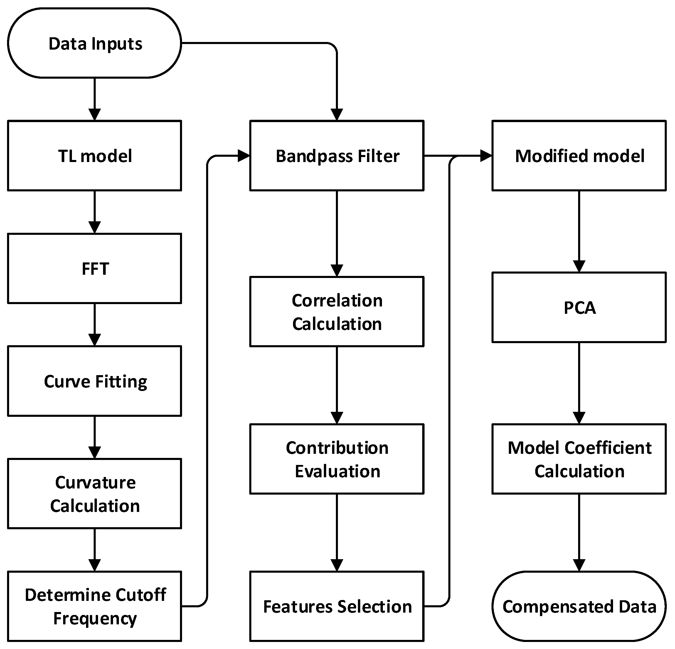
Figure 2. The original measurements and preliminary compensation results of TL model. (a) The original magnetic measurements of two magnetometers. (b) The preliminary compensation results of TL model.

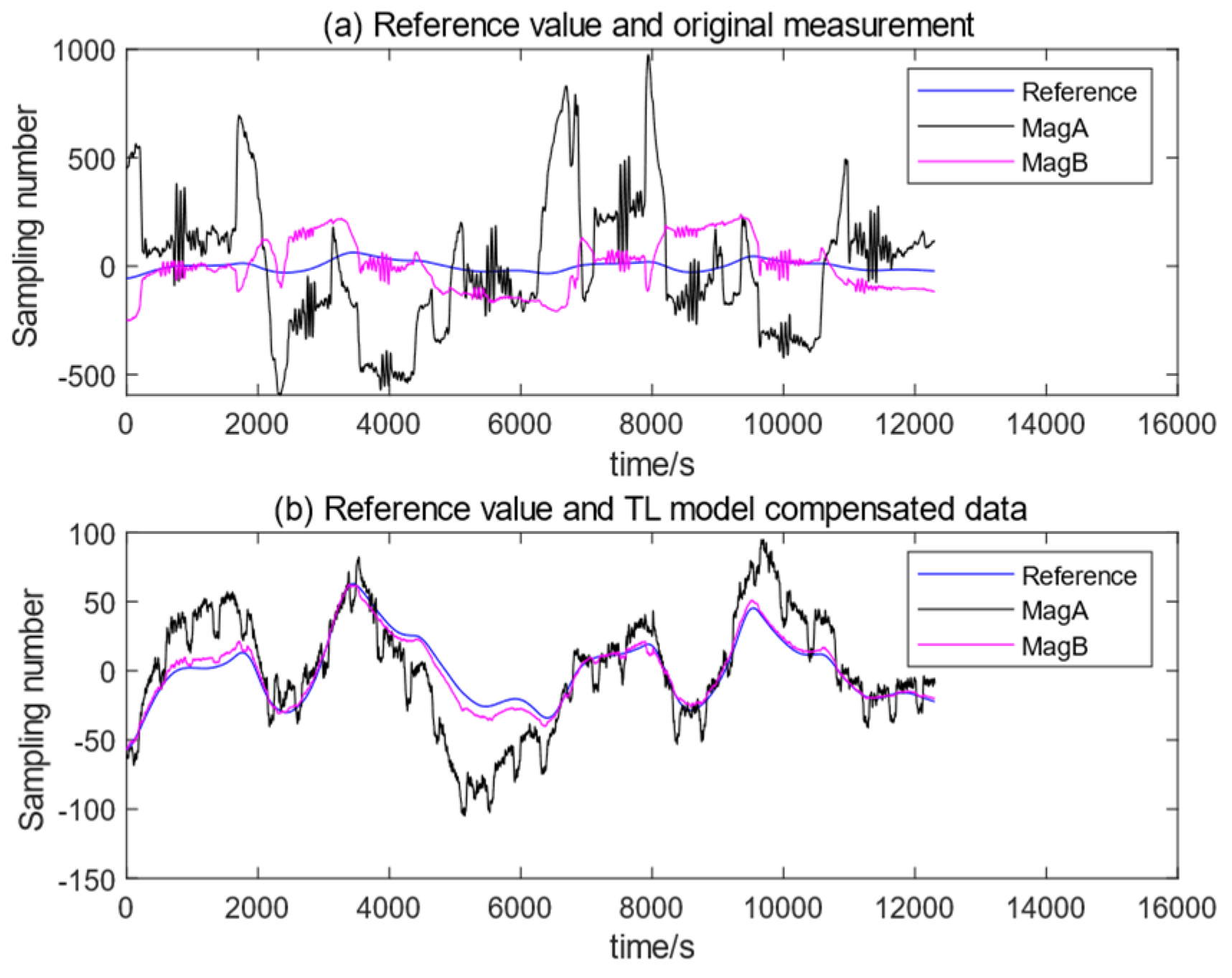
Figure 3. The frequency spectrum of reference value and T-L model compensation results. (a) The frequency spectrum of reference value. (b) The frequency spectrum of preliminary compensation results on MagA. (c) The frequency spectrum of preliminary compensation results on MagB.

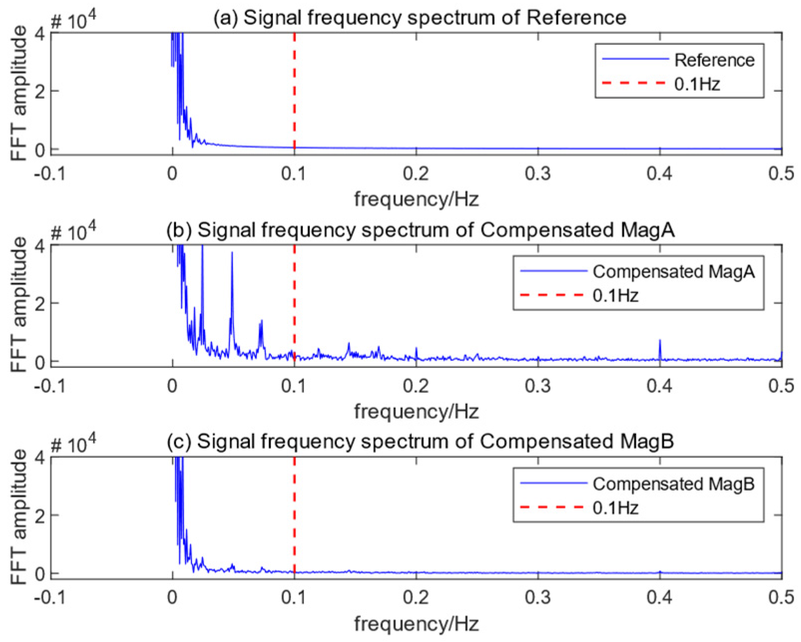
Figure 4. (a)Curve fitting of on MagA’s FFT result. (b) Curve fitting of on MagB’s FFT result.

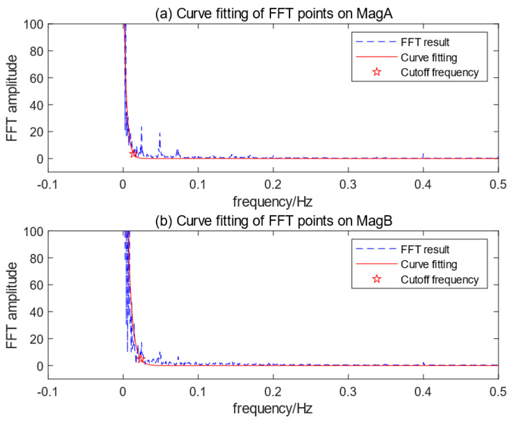
Figure 5. (a) Contribution of current on MagA. (b) Contribution of voltage on MagA. (c) Contribution of current on MagB. (d) Contribution of voltage on MagB.

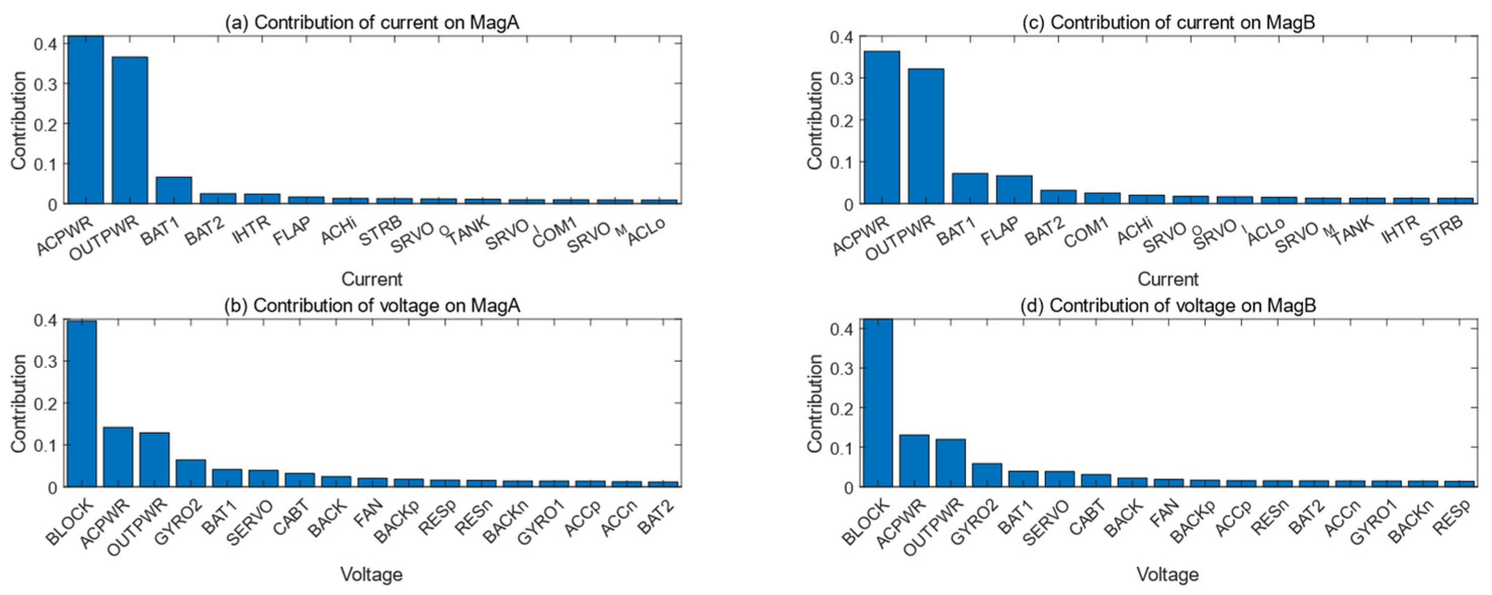
Figure 6. (a) Compensation results of MagA. (b) Compensation results of MagB.

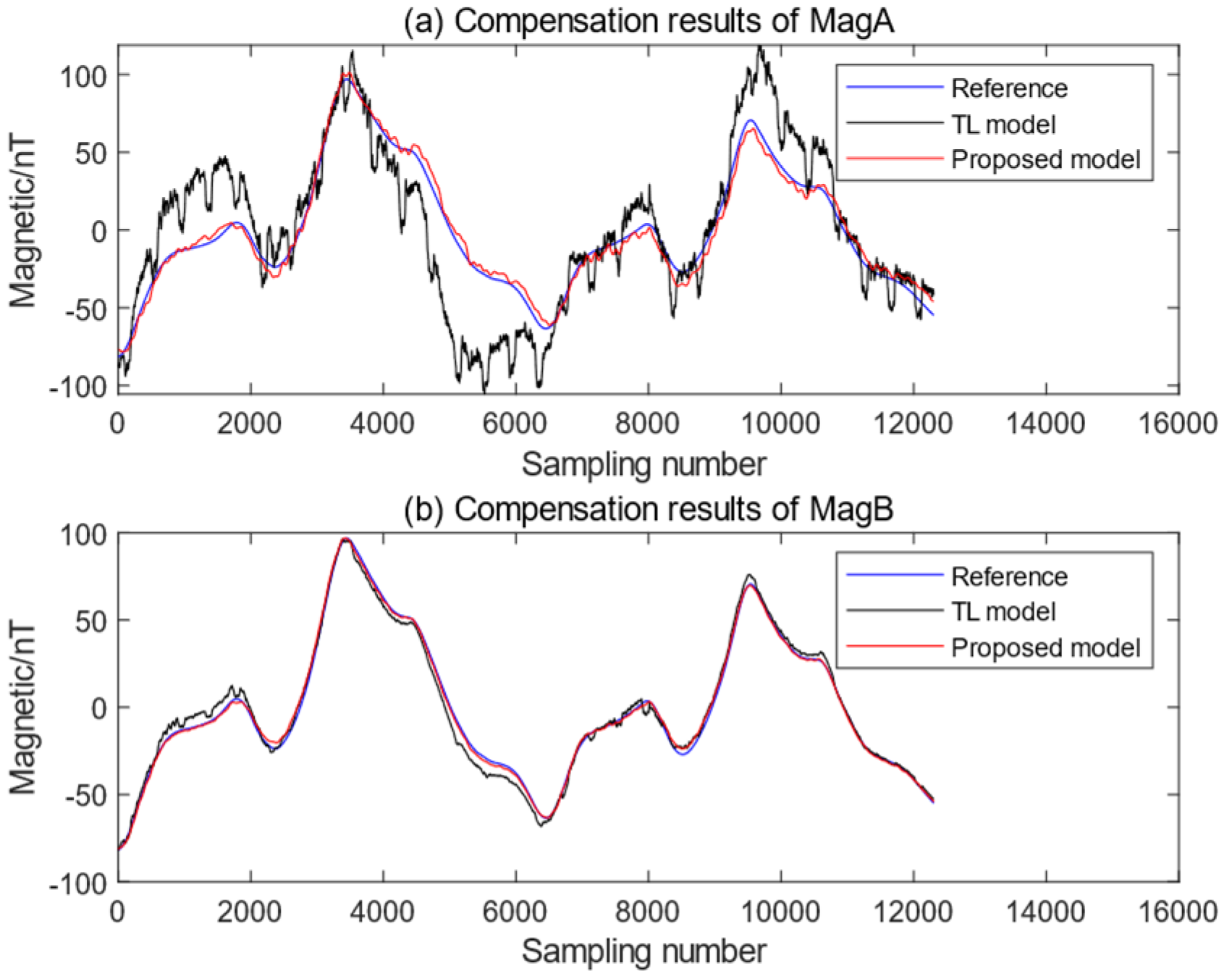
Figure 7. (a) Compensation results of smooth flight on MagA. (b) Compensation results ofsmooth flight on MagB.

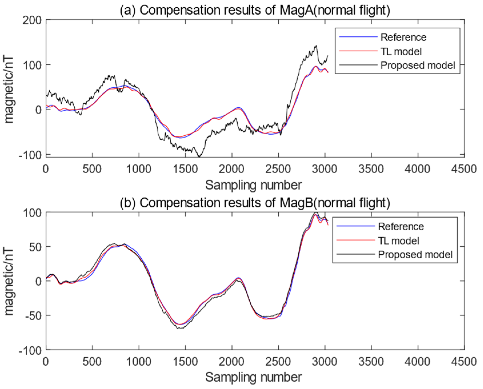
Table 1. The improvement of the modified model.

Method	MagA	MagB
Original measurements	326.45nT	102.37nT
TL model	27.71nT	4.30nT
Proposed method (model extension)	18.28nT	4.02nT
Proposed method (model extension, optimal cutoff frequency)	8.21nT	3.31nT
Proposed method (model extension, optimal cutoff frequency, features selection)	5.02nT	3.01nT
Proposed method (model extension, optimal cutoff frequency, features selection, PCA)	4.83nT	1.71nT

Table 2. The comparison of RMSE by the various methods.

Method	MagA	MagB
Original measurements	326.45nT	102.37nT
TL model	27.71nT	4.30nT
Method in reference [22]	20.01nT	3.86nT
Method in reference [23]	8.86nT	3.33nT
Proposed method	4.83nT	1.71nT

Disclaimer/Publisher’s Note: The statements, opinions and data contained in all publications are solely those of the individual author(s) and contributor(s) and not of MDPI and/or the editor(s). MDPI and/or the editor(s) disclaim responsibility for any injury to people or property resulting from any ideas, methods, instructions or products referred to in the content.

© 2024 by the authors. Licensee MDPI, Basel, Switzerland. This article is an open access article distributed under the terms and conditions of the Creative Commons Attribution (CC BY) license (http://creativecommons.org/licenses/by/4.0/).

Copyright: This open access article is published under a Creative Commons CC BY 4.0 license, which permit the free download, distribution, and reuse, provided that the author and preprint are cited in any reuse.

Downloads

189

Views

Comments

Subscription

Notify me about updates to this article or when a peer-reviewed version is published.

MDPI Initiatives

Important Links

Choose an area of interest and we will send you notifications of new preprints at your preferred frequency.

Disclaimer

A Modified Aeromagnetic Compensation Method Robust to In-Cabin OBE Interferences

Abstract

Keywords:

Subject:

1. Introduction

2. Proposed Aeromagnetic Compensation Method

2.1. Overall Method Framework

2.2. The Classical Aeromagnetic Compensation Model

2.3. The Modified Model for OBE Interferences

2.4. Cutoff Frequency Determination and Feature Selection

2.5. Estimation of Model Coefficients

3. Experiment Results

3.1. Dataset and Experiment Design

3.2. Experiment Results of Cutoff Frequency Determination

3.3. Experiment Results of Feature Selection

3.4. Compensation Results of Proposed Method

4. Discussion

5. Conclusions

Author Contributions

Funding

Acknowledgments

Conflicts of Interest

References

MDPI Initiatives

Important Links

Subscribe