
Submitted:
17 January 2024
Posted:
17 January 2024
You are already at the latest version
Abstract
To mitigate the interference of waves on offshore operation vessels, heave compensation systems find widespread application. The performance of heave compensation systems significantly influences the efficiency and safety of maritime operations. This paper establishes a mathematical model for winch-based active heave compensation system. It introduces a three-loop active disturbance rejection control (ADRC) strategy encompassing piston position control, winch speed control, and load displacement control, enabling real-time estimation and compensation of system disturbances, thereby enhancing the performance of the heave compensation system. To assess the effectiveness of this control strategy, the study employs Matlab/Simulink and AME Sim to construct a co-simulation model and conducts a comparative analysis with traditional PID control systems. The research findings indicate that the three-loop ADRC position control strategy consistently delivers superior compensation performance across various operational scenarios.
Keywords:
secondary component
; heave compensation system
; active disturbance rejection control
; position control strategy
1. Introduction
With the increasing scope and demand for ocean exploration, there is a growing demand for offshore engineering equipment. The Active Heave Compensation system (AHC) can be used to correct and compensate for the heave motion in the vertical direction that occurs during offshore operations of a vessel [1]. Applying this technology effectively avoids issues such as severe load motion, inaccurate positioning, wire rope breakage, and risks to the safety of personnel, thereby greatly improving the efficiency and safety of marine operations [2]. The actively controlled heave compensation system, consisting of a hydraulic transmission mechanism and a winch actuation mechanism, has a wide range of applications. This type of active compensation system has the advantages of a wide range of sea conditions suitable for compensation and high compensation accuracy. However, its disadvantages include a complex system structure, heavy reliance on the controller for compensation effectiveness, the requirement of an additional power source for the system itself, and high energy consumption [3].
To improve the performance of the active compensation system, scholars and companies from various countries have conducted research in areas such as mechanical structural design, control strategies, and numerical simulations [4,5,6]. Dabing et al. introduced a technology called secondary control hydraulic drive into the offshore crane system [7]. The secondary components can absorb the potential energy of the effective payload under pump conditions and convert the mechanical energy into hydraulic energy stored in an accumulator to save energy. Bosch Rexroth introduced a new type of hydraulic axial piston pump, the A4VSO and A4VSG, combined with a new secondary control HNC controller [8]. The system gives full consideration to the special characteristics of the use of the environment, driving the marine lifting winch for positive and negative rotation, so that the suspended weight can remain relatively static, to ensure that the equipment is stable and reliable when working at sea, to better meet the needs of practical applications. IHC, a company from the Netherlands, developed an active heavy compensation system [9]. This system utilizes a winch structure and can control the constant tension of the wire rope during lifting operations. The active compensation system has a compact size and improved control performance, showcasing its superiority in certain low-power conditions. However, its drawback is that it consumes a large amount of power, limiting its application in high-power working situations. Moslått integrated National Oilwell Varco's wave compensation crane and motor feedforward control technology to propose a hybrid active-passive heave compensation system [10]. This system demonstrates strong adaptability and flexibility.
To achieve high-precision compensation, effective control system schemes can be designed and appropriate control strategies can be selected [11]. There are many methods for traditional heave compensation system control, such as proportional-integral-derivative control (PID), sliding mode control (SMC), model predictive control (MPC), etc. In practical work, the AHC system is affected by external disturbances, including friction, unclear dynamic models, changes in effective payload weight, and parameter uncertainties. Using ordinary traditional controllers for complex nonlinear systems cannot achieve satisfactory control performance and accuracy [12].
Do and Pan first studied the nonlinear controller of AHC systems [13]. They designed a disturbance observer for the active heave compensation system in the electro-hydraulic system, which improved the control performance of the active heave compensation system. Küchler and Sawodny proposed a nonlinear control method consisting of feedforward and stable controllers to directly control the hydraulic drive winch of offshore cranes, decouple the load's motion from the one of the vessel, and achieve trajectory tracking of the payload in the coordinate system [14]. Hexiong Zhou proposed a robust hierarchical control scheme for a hydraulic-driven winch-based active heave compensation (AHC) system based on the combination of a nonlinear model predictive control (NMPC) strategy, to release the negative impact of the support vessels' vertical heave motion on the station-keeping and position tracking performance of TMS [15].
The Active Disturbance Rejection Controller (ADRC) can observe disturbances, which endows it with high robustness and the advantage of not depending on system models. This allows it to enhance the effectiveness of compensation and the ability to resist interferences [16,17]. As a result, ADRC is widely applied in various control systems. Zhou, R. and Neusypin, K. proposed a cascade ADRC control scheme for fixed-wing UAVs and tested the proposed control scheme through a series of simulations [18]. Even in the presence of strong disturbances, the ADRC control system demonstrates good robustness and accuracy. Messineo and Serrani proposed an adaptive controller for large offshore crane operations, relying on the use of an adaptive observer and two adaptive disturbance external models [19]. This controller effectively reduces the hydrodynamic impact load when the load enters the water. Li et al. applied the disturbance-attenuation-based control (ADRC), which is independent of mathematical models and has strong anti-interference capability, to tension control for heave compensation [20]. A newly developed second-order ADRC controller is used in the tension control strategy, leading to an improved compensation effect.
In this paper, the authors conducted research on the design and control of winch-based active heave compensation. They introduced secondary component and ADRC [21,22], then proposed a three-closed-loop ADRC position compensation strategy based on secondary component to resist external disturbances, which in turn improves the accuracy of the heave compensation system. The inner loop is the piston displacement control loop of the variable control cylinder, the middle loop is the winch rotation speed control loop, and the outermost loop is the load-displacement control loop. By properly setting the parameters of each ADRC loop, good control effects on load-displacement can be achieved. Finally, a joint simulation model is established using Matlab/Simulink and AMESim, and comparative analysis is performed with a PID control system to verify the proposed three-closed-loop ADRC position compensation strategy based on winch-type heave compensation system with a secondary component.
2. Dynamic Model of Heave Compensation System
The schematic diagram of a winch-type heave compensation system based on a secondary component is shown in Figure 1. The system consists of secondary components, a constant pressure oil source, a cable winding winch, variable control oil cylinders, and other modules. The utilization of secondary control techniques achieves significant energy recovery. This is mainly because the secondary component can switch between the operating conditions of a pump and a motor. When the output torque of the secondary component is greater than the load gravity, it operates in the motor condition, driving the load to rise and consuming energy. When the load gravity is greater than the output torque of the secondary component, it operates in the pump condition. The load drives the rotation of the secondary component, converting gravitational potential energy into hydraulic energy and storing it in the accumulator to achieve energy recovery.
2.1. Mathematical Modeling
The heave compensation system is mainly controlled through electro-hydraulic servo valves, variable control oil cylinders, secondary components, and a cable winding system. The displacement of the variable control oil cylinder piston is controlled by the electro-hydraulic servo valve, which in turn regulates hydraulic flow. The secondary component unit operates in a constant-pressure network, resulting in a proportional relationship between its output torque and displacement. By controlling the displacement of the variable control oil cylinder piston, the secondary component achieves variable displacement, thereby adjusting the winch's output torque. The balance between the load torque and the output torque is maintained through the cable winding system, ensuring controlled displacement and speed of the load. The displacement of the variable control oil cylinder piston, winch speed, and load-displacement are all regulated by the ADRC controller, with the control structure being a three-closed-loop ADRC position control, as illustrated in Figure 2.
2.1.1. The model of the electro-hydraulic servo valve
The mathematical model of the electro-hydraulic servo valve, after simplification, is typically represented as:
In the equation, Qsf represents the output flow, I is the coil input current, Kv is the flow gain, s is the Laplace operator, ωn is the natural frequency, and ξn is the damping ratio. Due to its inherent frequency generally being much higher than the system bandwidth, it can be approximated as a proportional link:
2.1.2. Variable control oil cylinder
The continuity equation for fluid flow is:
In the equation, q is the flow entering the high-pressure chamber of the cylinder, Ag is the effective piston area inside the cylinder, xg is the piston displacement, Ct is the total leakage coefficient, p is the pressure difference between the high-pressure and low-pressure chambers, Vt is the total volume of the two chambers, βe is the volumetric modulus of oil, Ci is the internal leakage coefficient, and Ce is the external leakage coefficient.
Further derivation leads to the force balance equation for the variable control oil cylinder:
In the equation, mg represents the total mass of the moving components, Bg is the viscous damping coefficient, kg is the spring stiffness, and Ffg is the resistance force acting on the piston.
2.1.3. Secondary component displacement
In the equation, Der represents the displacement, Dermax is its maximum displacement, and xgmax is the maximum displacement of the piston.
The force balance equation for the motor operating condition is:
The force balance equation for the pump operating condition is:
In the equation, ps represents the constant pressure of the oil supply, Jer is the rotational inertia converted to the output shaft, θer is the main shaft rotation angle of the secondary component, Ber is the viscous damping coefficient converted to the output shaft, and ML is the external load torque.
2.1.4. Cable winding system
The displacement equation of the cable-driven load in the vertical direction is:
In the equation, xl represents the displacement of the load in the vertical direction, xl0 is the initial position of the load, xh is the displacement due to the heave of the ship, ijt is the reduction ratio of the gearbox, R is the radius of the winch drum, ∆l is the elongation of the cable, ∆ld is the dynamic elongation of the cable, and ∆ls is the static elongation of the cable.
In the air, the kinetic equations for the motion of the load driven by the cable is:
In the equation, meq represents the equivalent mass of the load and cable, kl is the cable's elastic coefficient, and Cl is the cable's damping coefficient.
2.2. Simulation model and parameter settings
The control methods applied to practical physical systems must undergo feasibility verification based on computer simulation before being implemented in engineering applications. For the studied winch-type heave compensation system, a combined simulation model of the electro-hydraulic control system is established using Matlab/Simulink and AMESim. According to the components of the experimental platform for the winch-type heave compensation system, the constructed model is mainly divided into two parts: the hydraulic system main part is built in AMESim, and the control system part is completed in Matlab/Simulink.
Due to the uncertainty of certain time-varying parameters, there may inevitably be some deviations. Here, it is explicitly stated the assumed premises under which this simulation model is established:
- The system operates in an ideal constant temperature and constant pressure hydraulic environment. The hydraulic components and pipelines are sufficiently rigid, and there is no pressure loss along the pipeline.
- The hydraulic oil is considered to be incompressible, with constant density and viscosity.
- Friction forces at various locations such as the cable and valve spool are assumed to be constant and do not vary with operating conditions and temperature changes.
The selection of main component sub-models for the AMESim hydraulic system simulation model built in this paper is shown in Table 1 below:
The main parameters used in the simulation are listed in Table 2. Other parameters are selected conventionally for hydraulic system design.
3. Three-Closed-Loop ADRC Position Control Strategy Design
3.1. ADRC Controller Design and Composition
The Active Disturbance Rejection Control (ADRC) was invented by Jingqing Han in the direction of improving the PID controller [22]. Its basic principle is to extract real-time disturbance information from input and output signals and compensate for it through control force to achieve effective control. It has excellent disturbance rejection capabilities. The ADRC control structure is shown in Figure 3. below.
Taking the heave compensation system as the controlled object, its algorithm mainly consists of four parts: tracking differentiator, extended state observer, nonlinear state error feedback law, and disturbance estimation compensation.
3.1.1. The Track Differentiators, TD
According to the reference signal r(t) and the given transition process r₁(t), compute its derivative signal r₂(t). In discrete form, it can be expressed as follows:
Where r is the velocity factor, and a larger value approaches the speed faster; h₀ is the filtering factor; h is the integration step size, typically h0 can be equal to h, but to reduce overshoot and oscillations, h₀ is usually taken greater than h.
fhan is the maximum speed control function, which has the following form:
The expression for the fsg function is:
3.1.2. Extended State Observer, ESO
The Extended State Observer (ESO) is used to observe the state and disturbance of the controlled object. Its specific expression is as follows:
The expression for the nonlinear function fal(e, α, δ) is as follows:
The parameters β01, β02, and β03 are observer gain parameters. The setting of these parameters can be determined based on the bandwidth method given by Gao Zhiqiang [23], as follows:
Where ω is the observer bandwidth. z₁ is the estimated state signal, z₂ is the estimated state velocity signal, and z₃ is the estimated state acceleration signal.
3.1.3. Nonlinear States Error Feed-Back, NLSEF
The system's state error is determined by the difference between the outputs of ESO and TD. Then, the control law is determined based on the state error, as shown below:
The equation includes u0, which represents the error feedback control signal.
3.1.4. Disturbance Estimation Compensation
The feedback control signal for the state error is compensated using the disturbance estimation value to determine the final control input to the controlled object. The form is as follows:
In the equation, b₀ is the compensation factor. Increasing b₀ can reduce oscillations, but it will simultaneously decrease the compensation for disturbances, affecting disturbance suppression effectiveness.
3.2. Controller Design and Parameter Setting
The design of the ADRC controller follows the principle of "inner loop before outer loop" to design a three-closed-loop position controller. The inner loop is the control loop for the piston displacement of the variable control cylinder, the middle loop is for the winch rotational speed control, and the outermost loop is for the load-displacement control. The parameter tuning begins with the inner control loop. By directly comparing the input signal and the output feedback signal of the inner loop, parameter tuning of a single-loop ADRC controller is achieved. Then, the parameter tuning continues with the next loop, the rotational speed control loop. Since the inner loop has completed parameter tuning, it acts as a gain structure with a value of "1" in the control system, and its influence on the next loop can be neglected. Following the same method, parameter tuning is sequentially completed for the middle rotational speed loop and the outermost displacement loop.
Based on this, three second-order ADRC controllers are separately designed to construct the piston displacement loop, winch rotation speed loop, and load displacement loop, forming the three-closed-loop ADRC control. The control structure is illustrated in Figure 4.
Each controller structure is roughly the same. The input signal is denoted as r(t). It first undergoes processing through a Tracking-Differentiator (TD) to obtain the differential signal and smooth command signals r₁(t) and r₂(t). The second-order Extended State Observer (ESO), established for each system, observes the feedback signals. Z₁ represents the estimated state signal, Z₂ is the estimated state velocity signal, and Z₃ is the estimated state acceleration signal. The observer gain parameters β₀₁, β₀₂, and β₀₃ are adjusted through the gain scheduling method, and the tuning of these parameters can be determined using the bandwidth method provided by Gao Zhiqiang [23]. The specific control parameters are listed in Table 3. Finally, the signals r₁(t) and r₂(t) from the Tracking Differentiator (TD) and the signals Z from the Extended State Observer (ESO) are input into the Nonlinear State Error Feedback (NLSEF) controller. By adjusting the compensation factor b₀ error and disturbance are estimated and compensated.
The internal structure of the ADRC controller and the simulation model for the three-closed-loop ADRC position control are shown in Figure 5 and Figure 6, respectively. Using the bandwidth method, the parameters of each ADRC controller loop are tuned to achieve good control performance for load displacement.
4. Simulation Experiment Research and Analysis
4.1. Step Response Analysis
To compare the dynamic performance of the three-closed-loop PID control system and the three-closed-loop ADRC control system, a step signal is applied to the designed simulation system model. As shown in Figure 7, the given step signal has an amplitude of 1 meter, starting from 1 second.
Input the simulation results into MATLAB, then use the stepinfo function to extract the step response metrics for each curve. As shown in Table 4.
The parameters of the PID controller consist of two sets: one set for the no overshoot condition and another set that, with slight adjustment, introduces a small overshoot. By comparing the step response curves of the two PID sets with the step response curve of the ADRC, it is evident that the three-closed-loop ADRC control system has a faster response speed. Even when adjusting the PID parameters to induce overshoot, the system's response does not significantly accelerate. This indicates that the classical PID controller indeed faces a trade-off between speed and overshoot. In contrast, the three-closed-loop ADRC controller designed in this paper effectively addresses this trade-off.
4.2. Sine Response Analysis
Taking a condition close to sea state 3, a sine curve with an amplitude of 0.5m and a period of 10s was selected for simulation, as shown in Figure 8. The black curve represents the input desired curve, i.e., the given sine command signal. The blue solid line represents the load-displacement curve output by the three-closed-loop PID control system, while the green solid line represents the load-displacement curve under the three-closed-loop ADRC control system. The blue dashed line represents the load-displacement error curve under the three-closed-loop PID control system, and the green dashed line represents the load-displacement error curve output by the three-closed-loop ADRC control system. From the graph, it can be observed that during the startup phase, the three-closed-loop ADRC control system exhibits better dynamic performance compared to the three-closed-loop PID control system. It can quickly follow the input sine command signal, and during the subsequent tracking motion, the phase lag between the tracking curve of the three-closed-loop ADRC control system and the input desired curve is smaller compared to the three-closed-loop PID control system.
The error statistics adopt the Root Mean Square Error Compensation Rate ζ and the maximum error in heave compensation ∆ to express the efficiency and accuracy of the compensation strategy.
Define the heave compensation Root Mean Square Error Compensation Rate:
Maximum error in heave compensation:
In the equation, T is the statistical duration, x is the amplitude of the desired curve at time t, and x^ is the amplitude of the target curve at time t.
Based on the simulation results, when a sine curve with an amplitude of 0.5m and a period of 10s is input into the systems, ignoring the initial startup phase, the maximum error for the three-closed-loop PID control system is 0.061m, and for the three-closed-loop ADRC control system, it is 0.045m. The compensation rates for the three-closed-loop PID control system and the three-closed-loop ADRC control system are 83.46% and 91.52%, respectively. The designed three-closed-loop ADRC controller exhibits better compensation performance under this operating condition.
4.3. South China Sea Ship Heave Motion Curve Response Analysis
The simulation of the heave motion curve responses for the South China Sea ship is conducted for the three-closed-loop ADRC position control system and the no overshoot three-closed-loop PID position control system. The results are shown in Figure 9 and Figure 10. Each curve corresponds to the input and output signals, and they remain consistent with the sine response curves.
According to the simulation results, the maximum amplitude of the measured heave motion for the ship is 0.374m. Under the compensation of the three-closed-loop PID control system, the maximum load displacement error is ±0.079m, with a compensation rate of 75.16%. Under the compensation of the three-closed-loop ADRC control system, the maximum load displacement error is ±0.061m, with a compensation rate of 90.81%. The compensation rate has increased by 15.65%. Therefore, whether in step response, sine response, or the response to the measured heave motion of the ship, the designed three-closed-loop ADRC position control system exhibits faster dynamic characteristics and smaller tracking errors.
Figure 11 shows a local magnification of the simulation curve of the measured heave motion for the ship under the three-closed-loop control system. From the figure, it can be observed that there is a phase delay of less than 0.2s in the system. This is due to the large inertia of the winch compensation system, resulting in response delay in the system, and the presence of delay in the ship heave motion sensor, causing phase delay, thereby affecting the accuracy of position compensation. This issue can be improved by predicting the heave motion of the ship.
5. Conclusions
For the winch-based active heave compensation system, a three-closed-loop ADRC position compensation strategy based on winch-type heave compensation system with a secondary component is proposed. The ADRC controllers for each loop compensate for the total disturbance information extracted in real time from the input and output signals, achieving better control performance and excellent disturbance rejection capability. By tuning the parameters of each ADRC loop, a superior control effect on load displacement is ultimately achieved, enhancing the compensation performance.
The proposed the three-closed-loop ADRC position compensation strategy based on winch-type heave compensation system with a secondary component achieves accurate and rapid position tracking control under various sea conditions. Under the condition of the maximum amplitude of 0.374m in the measured heave motion of the ship in the South China Sea, the winch-based heave compensation system with the secondary component, using the three-closed-loop ADRC position control, achieves a maximum load displacement error of ±0.061m with a compensation rate of 90.81%, demonstrating excellent heave compensation performance.
Author Contributions
Conceptualization, S.L. and F.Y.; methodology, Q.W. and F.Y.; software, Q.W. and L.Q.; validation, Q.W., Y.L. and Z.G.; formal analysis, Q.W. and F.Y; investigation, Q.W. and F.Y; resources, S.L. and Y.L.; data curation, L.Q. and Q.W.; writing—original draft preparation, Q.W. and F.Y; writing—review and editing, S.L., Q.W. and F.Y.; visualization, Z.G.; project administration, S.L. and F.Y; All authors have read and agreed to the published version of the manuscript.
Funding
This research was funded by the National Natural Science Foundation of China (General Program, grant number 2021SDDR228), Excellent Youth Foundation of Shandong Scientific Committee (grant number B8D9B198A48D6A25E053BE07C2CAC8E8).
Institutional Review Board Statement
Not applicable.
Informed Consent Statement
Not applicable.
Data Availability Statement
Not applicable.
Conflicts of Interest
The authors declare no conflict of interest.
References
- Woodacre, J.K.; Bauer, R.J.; Irani, R.A. A Review of Vertical Motion Heave Compensation Systems. Ocean Eng. 2015, 104, 140–154. [CrossRef]
- Petillot, Y.R.; Antonelli, G.; Casalino, G.; Ferreira, F. Underwater Robots: From Remotely Operated Vehicles to Intervention-Autonomous Underwater Vehicles. IEEE Robot. Autom. Mag. 2019, 26, 94–101. [CrossRef]
- Yu, H.; Chen, Y.; Shi, W.; Xiong, Y.; Wei, J. State Constrained Variable Structure Control for Active Heave Compensators. IEEE Access 2019, 7, 54770–54779. [CrossRef]
- Woo, N.-S.; Kim, H.-J.; Han, S.-M.; Ha, J.-H.; Huh, S.-C.; Kim, Y.-J. Evaluation of the Structural Stability of a Heave Compensator for an Offshore Plant and the Optimization of Its Shape. J. Nanosci. Nanotechnol. 2020, 20, 263–269. [CrossRef]
- Xie, T.; Zou, D.; Huang, L.; Liu, D. Modelling and Simulation Analysis of Active Heave Compensation Control System for Marine Winch. In Proceedings of the 2021 IEEE 4th International Electrical and Energy Conference (CIEEC); IEEE: Wuhan, China, May 28 2021; pp. 1–6. [CrossRef]
- Jakubowski, A.; Milecki, A. The Investigations of Hydraulic Heave Compensation System. In Automation 2018; Szewczyk, R., Zieliński, C., Kaliczyńska, M., Eds.; Advances in Intelligent Systems and Computing; Springer International Publishing: Cham, 2018; Vol. 743, pp. 380–391 ISBN 978-3-319-77178-6. [CrossRef]
- Dabing, Z.; Jianzhong, W.; Xin, L. Ship-Mounted Crane’s Heave Compensation System Based on Hydrostatic Secondary Control. In Proceedings of the 2011 International Conference on Mechatronic Science, Electric Engineering and Computer (MEC); IEEE: Jilin, August 2011; pp. 1626–1628. [CrossRef]
- Busquets, E.; Ivantysynova, M. Adaptive Robust Motion Control of an Excavator Hydraulic Hybrid Swing Drive. SAE Int. J. Commer. Veh. 2015, 8, 568–582. [CrossRef]
- Liu, T.; Iturrino, G.; Goldberg, D.; Meissner, E.; Swain, K.; Furman, C.; Fitzgerald, P.; Frisbee, N.; Chlimoun, J.; Van Hyfte, J.; et al. Performance Evaluation of Active Wireline Heave Compensation Systems in Marine Well Logging Environments. Geo-Mar. Lett. 2013, 33, 83–93. [CrossRef]
- Moslått, G.-A.; Rygaard Hansen, M.; Padovani, D. Performance Improvement of a Hydraulic Active/Passive Heave Compensation Winch Using Semi Secondary Motor Control: Experimental and Numerical Verification. Energies 2020, 13, 2671. [CrossRef]
- Zinage, S.; Somayajula, A. Deep Reinforcement Learning Based Controller for Active Heave Compensation. IFAC-Pap. 2021, 54, 161–167. [CrossRef]
- Tianxiang, M.; Yi, Y.; Jianbo, C.; Guihong, Z.; Yuanpei, Y.; Jianshan, W.; Haiqin, G.; Hui, Y. Design of Heave Compensation Control System Based on Variable Parameter PID Algorithm. In Proceedings of the 2018 Chinese Control And Decision Conference (CCDC); IEEE: Shenyang, June 2018; pp. 825–829. [CrossRef]
- Do, K.D.; Pan, J. Nonlinear Control of an Active Heave Compensation System. Ocean Eng. 2008, 35, 558–571. [CrossRef]
- Kuchler, S.; Sawodny, O. Nonlinear Control of an Active Heave Compensation System with Time-Delay. In Proceedings of the 2010 IEEE International Conference on Control Applications; IEEE: Yokohama, Japan, September 2010; pp. 1313–1318. [CrossRef]
- Zhou, H.; Cao, J.; Yao, B.; Lian, L. Hierarchical NMPC–ISMC of Active Heave Motion Compensation System for TMS–ROV Recovery. Ocean Eng. 2021, 239, 109834. [CrossRef]
- Li, Z.; Ma, X.; Li, Y.; Meng, Q.; Li, J. ADRC-ESMPC Active Heave Compensation Control Strategy for Offshore Cranes. Ships Offshore Struct. 2020, 15, 1098–1106. [CrossRef]
- Shuguang, L.; Wuyang, C.; Kecheng, W.; Jia, J. An ADRC-Based Active Heave Compensation for Offshore Rig. In Proceedings of the 2020 Chinese Control And Decision Conference (CCDC); IEEE: Hefei, China, August 2020; pp. 2979–2984. [CrossRef]
- Zhou, R.; Neusypin, K.A. ADRC-Based UAV Control Scheme for Automatic Carrier Landing. In Proceedings of the 15th International Conference “Intelligent Systems” (INTELS’22); MDPI, October 9 2023; p. 66. [CrossRef]
- Messineo, S.; Serrani, A. Offshore Crane Control Based on Adaptive External Models. Automatica 2009, 45, 2546–2556. [CrossRef]
- Li, M.; Gao, P.; Zhang, J.; Gu, J.; Zhang, Y. Study on the System Design and Control Method of a Semi-Active Heave Compensation System. Ships Offshore Struct. 2018, 13, 43–55. [CrossRef]
- Röper, R. Ölhydraulik und Pneumatik. In Dubbel; Beitz, W., Küttner, K.-H., Eds.; Springer Berlin Heidelberg: Berlin, Heidelberg, 1987; pp. 597–616 ISBN 978-3-662-06779-6. [CrossRef]
- Han, J. From PID to Active Disturbance Rejection Control. IEEE Trans. Ind. Electron. 2009, 56, 900–906. [CrossRef]
- Zhiqiang Gao; Yi Huang; Jingqing Han An Alternative Paradigm for Control System Design. In Proceedings of the Proceedings of the 40th IEEE Conference on Decision and Control (Cat. No.01CH37228); IEEE: Orlando, FL, USA, 2001; Vol. 5, pp. 4578–4585. [CrossRef]
Figure 1.
Winch heave compensation system based on a secondary component.
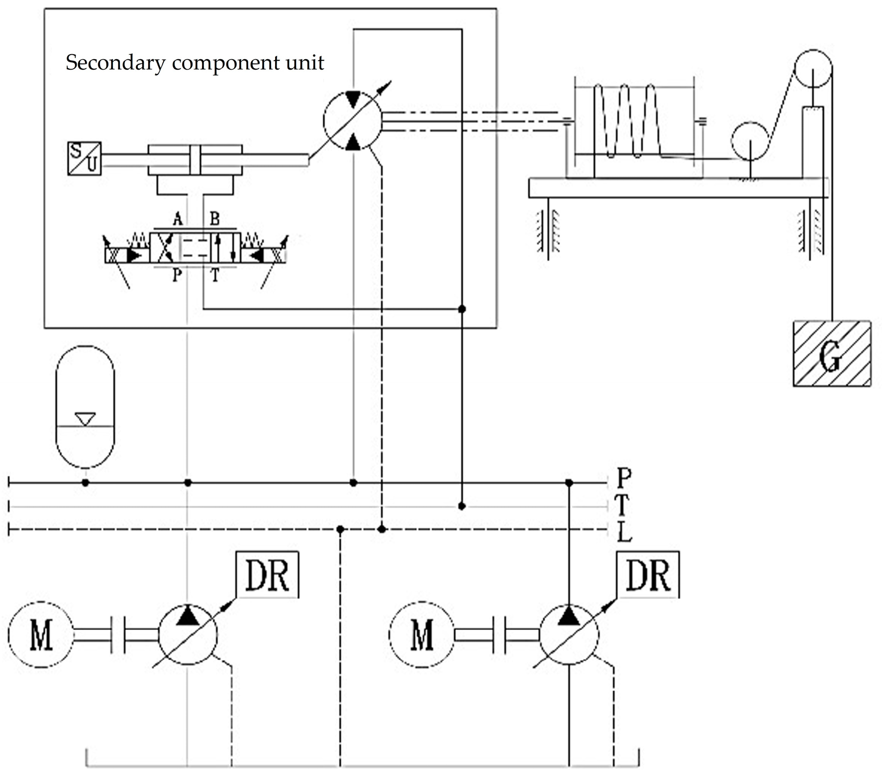
Figure 2.
Structure diagram of heave compensation control.
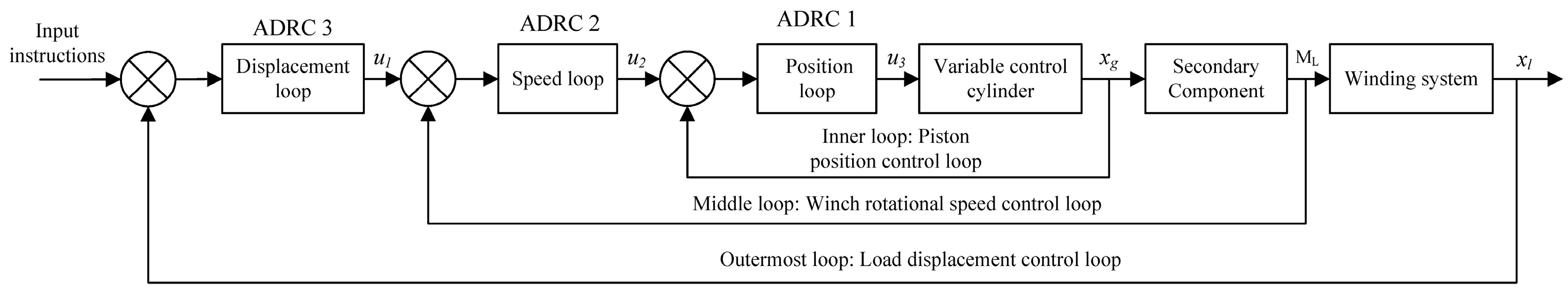
Figure 3.
ADRC algorithm flow chart.
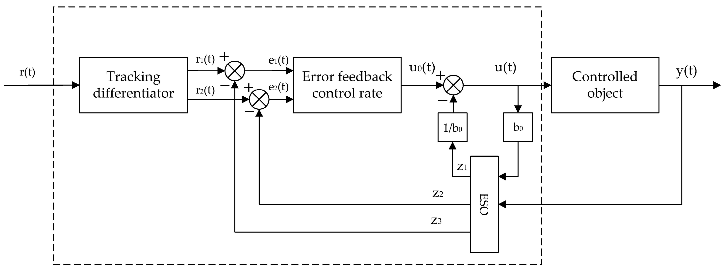
Figure 4.
Three closed-loop ADRC control block diagram.
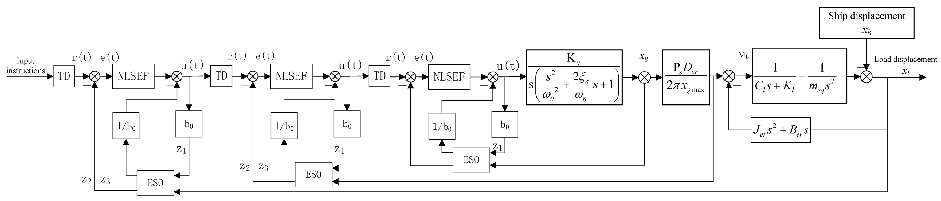
Figure 5.
The internal structure of the ADRC controller.
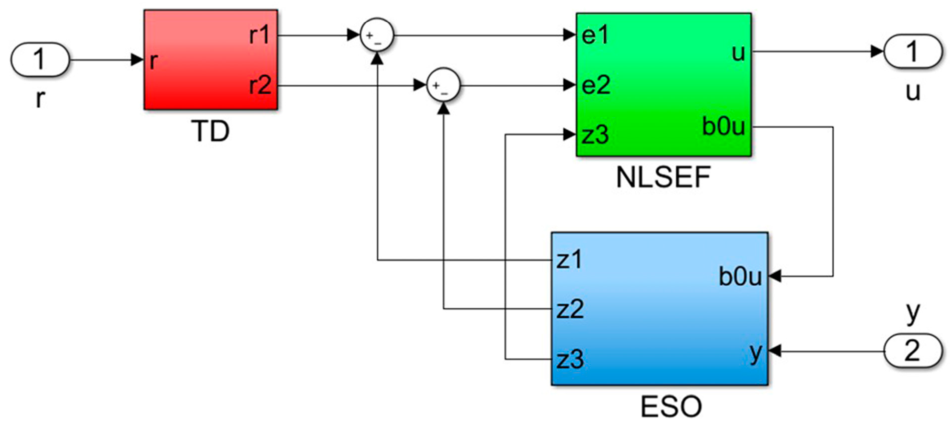
Figure 6.
Three-closed-loop ADRC position control simulation model.
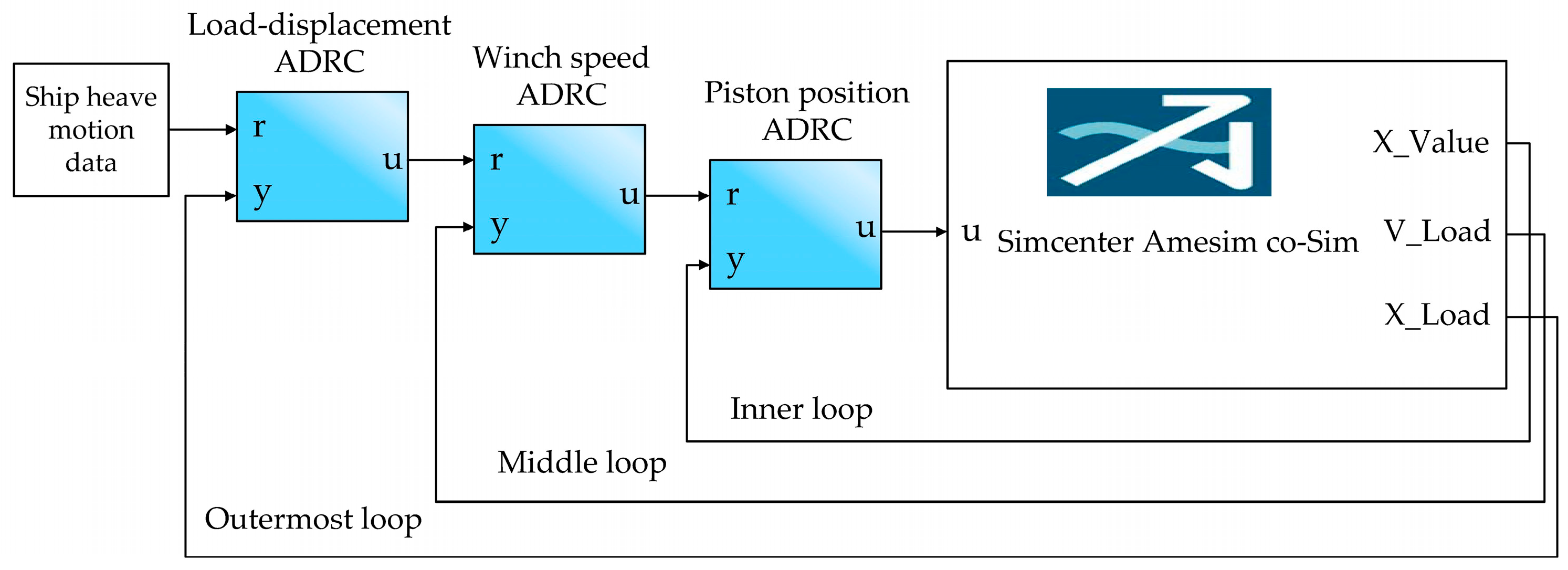
Figure 7.
Simulation curve of step response of three-closed-loop control system.
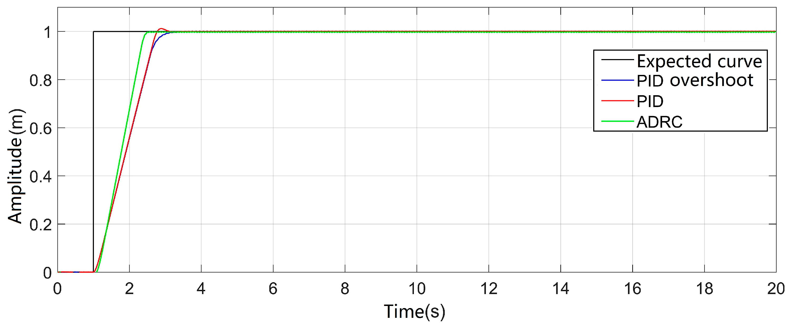
Figure 8.
The sinusoidal response curve of three-closed-loop position control system with amplitude 0.5m and period 10s.
Figure 8.
The sinusoidal response curve of three-closed-loop position control system with amplitude 0.5m and period 10s.
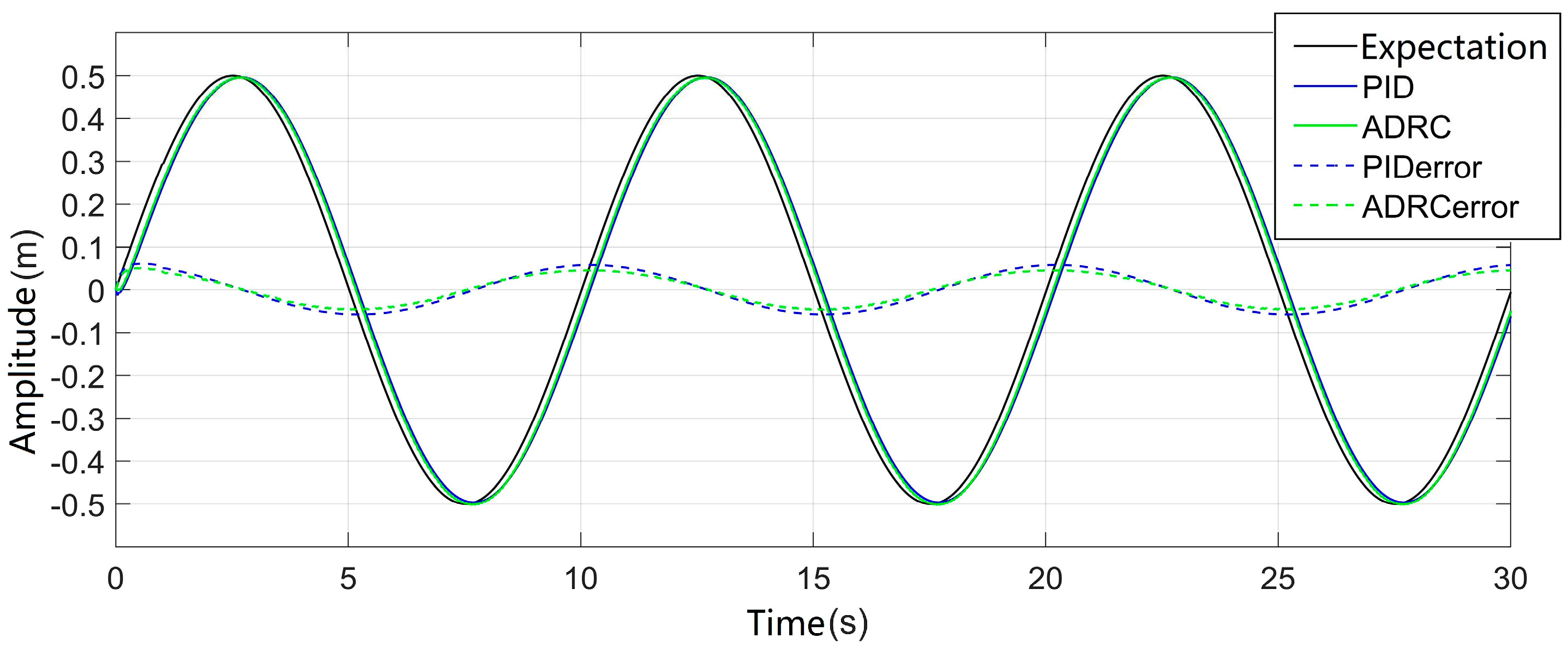
Figure 9.
Simulation curve of measured ship heave curve of three-closed-loop control system.
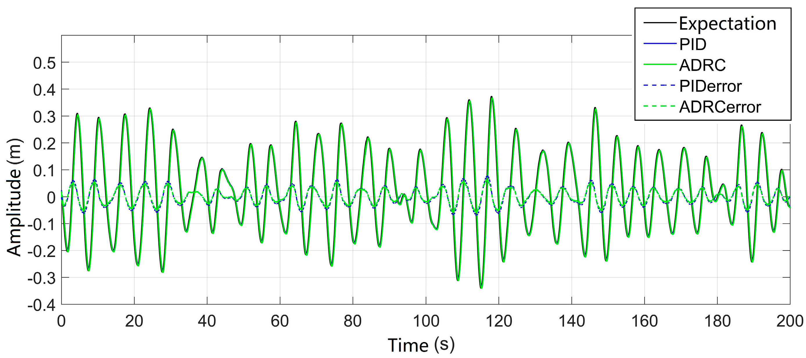
Figure 10.
Simulation error curve of ship heave motion measured by the three-closed-loop control system.
Figure 10.
Simulation error curve of ship heave motion measured by the three-closed-loop control system.
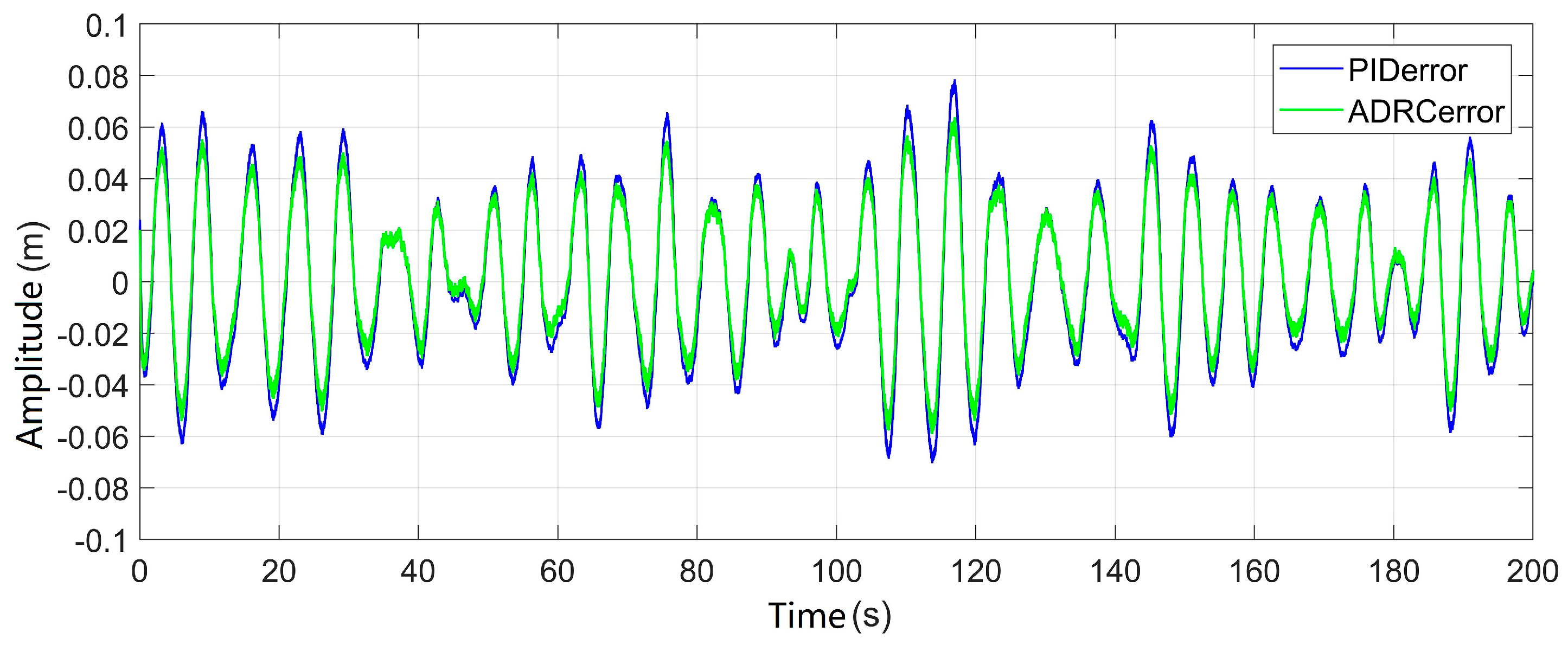
Figure 11.
Local magnification of the simulation curve for the heave motion of the ship under the three-closed-loop control system.
Figure 11.
Local magnification of the simulation curve for the heave motion of the ship under the three-closed-loop control system.
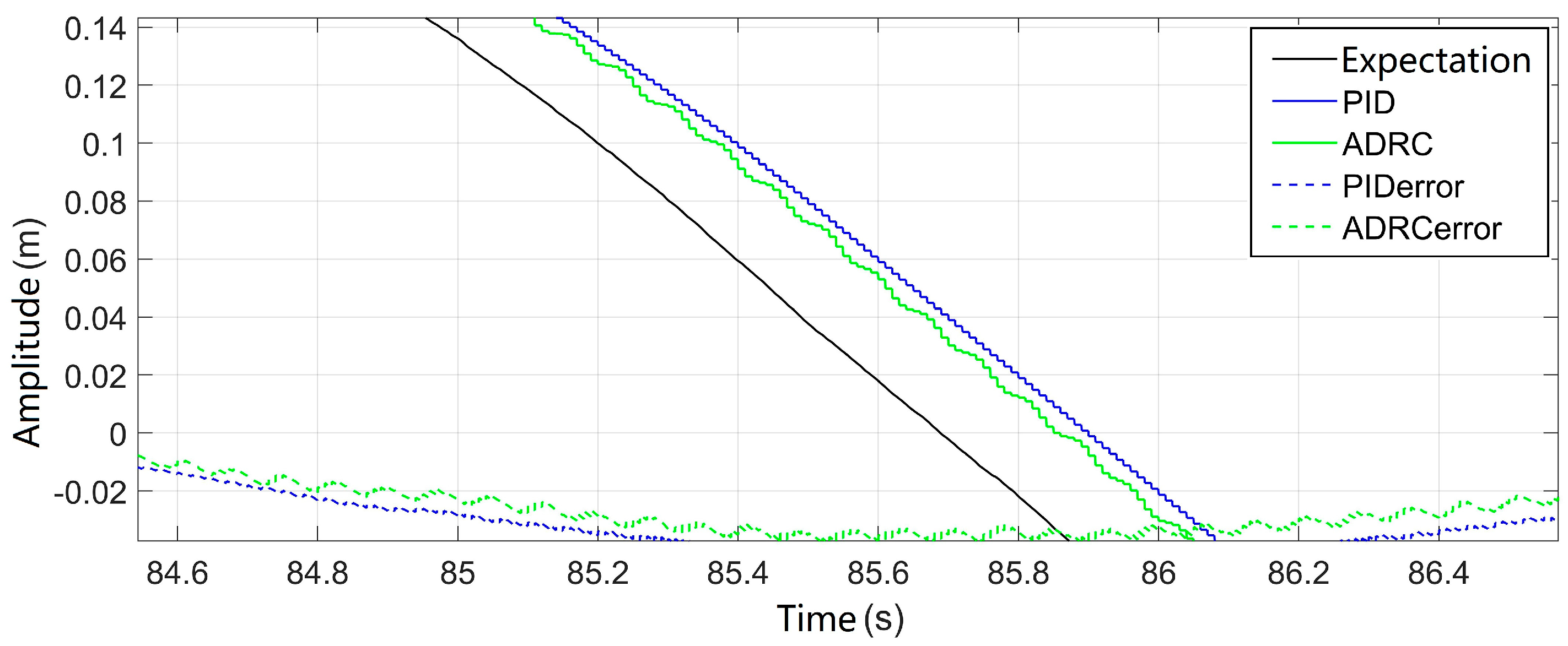

Table 1.
Sub-models of the main components in the hydraulic system simulation model.
| Main components | Sub-model | Functional description |
|---|---|---|
| Motor | PM000 | Standard Electric Motor |
| Pump | PP01 | Constant Pressure Variable Pump |
| Servo Valve | SV00 | Three-Position Four-Way Directional Valve |
| Relief Valve | RV012 | Safety Valve |
| Accumulator | HA000 | Diaphragm-type Accumulator |
| Variable cylinder Spring Chamber | BAP016 | Variable cylinder Reset Function Chamber |
| Variable cylinder Piston Chamber | BAF01 | Variable cylinder Control Function Chamber |
| Mass Block | MECMAS21/MAS001 | Variable cylinder Mass Property Simulation |
| Hydraulic Motor | HYDVPM01 | Bidirectional Variable Hydraulic Motor |
| Winch | WINCH01 | Ideal Winch |
| Cable or Wire Rope | MECROPE0/REND001 | Rigid Rope |
Table 2.
Main parameters of the simulation model.
| Parameter Name | Value | Unit |
|---|---|---|
| Hydraulic motor displacement Der | 40 | mL/r |
| Maximum motor speed nmdmax | 664 | r/min |
| Gearbox reduction ratio ijt | 26.4 | — |
| Winch drum radius R | 190 | mm |
| System pressure ps | 18 | MPa |
| Accumulator volume V | 20 | L |
Table 3.
Three-closed-loop ADRC controller parameters.
| Parameters | h | rTD | rNLSEF | β01 | β02 | β03 | b0 |
|---|---|---|---|---|---|---|---|
| Inner loop ADRC | 0.001 | 1×10⁷ | 5×10⁷ | 10000 | 1×10⁷ | 1×10⁸/3 | 1×10⁶ |
| Middle loop ADRC | 0.001 | 900 | 1×10⁵ | 10000 | 3.75×10⁷ | 6.25×10¹⁰ | 780 |
| Outermost loop ADRC | 0.001 | 900 | 4.5×10⁵ | 10000 | 3.75×10⁷ | 6.25×10¹⁰ | 7500 |
Table 4.
Step response index evaluation table.
| Parameters | Rise Time (s) | Peak Time (s) | Maximum Overshoot |
Settling Time (s) |
|---|---|---|---|---|
| No Overshoot PID | 1.3445 | 2.3400 | 0 | 1.7077 |
| Overshoot PID | 1.3347 | 1.8900 | 1.18% | 1.6563 |
| ADRC | 1.0257 | 1.5700 | 0 | 1.3532 |
* Note: Settling time is the time required for the response curve to reach and stay within a 5% error range of the steady-state value.
Disclaimer/Publisher’s Note: The statements, opinions and data contained in all publications are solely those of the individual author(s) and contributor(s) and not of MDPI and/or the editor(s). MDPI and/or the editor(s) disclaim responsibility for any injury to people or property resulting from any ideas, methods, instructions or products referred to in the content. |
© 2024 by the authors. Licensee MDPI, Basel, Switzerland. This article is an open access article distributed under the terms and conditions of the Creative Commons Attribution (CC BY) license (http://creativecommons.org/licenses/by/4.0/).
Copyright: This open access article is published under a Creative Commons CC BY 4.0 license, which permit the free download, distribution, and reuse, provided that the author and preprint are cited in any reuse.


