Submitted:
11 January 2024
Posted:
11 January 2024
You are already at the latest version
Abstract
This scientific paper presents a comprehensive investigation into transient Fourier analysis in some electrical engineering applications. The article deals with two effective approaches for solving transient analysis whose application is rather novel. The first contribution uses combined the Fourier series analytic Laplace-Carson (LC) transform methods in the complex domain using complex time vectors, thereby significantly simplifying the calculation of the original function. As the inverse transform goes back into the time domain, it employs the Cauchy-Heaviside (CH) method. The second contribution uses the Fourier transform (FΤ)for transient analysis of a power converter electrical circuit with the passive and the active load. The method of complex conjugated amplitudes is used for steady-state analysis. Both contributions represent a new approach to this paper. The starting point is the Fourier series/expansions, computation of the Fourier coefficients, then continuing by solving the steady and transient states of the system and confirming the transient states using the Fourier transform. To validate our findings, the worked-out analytical results are verified by modelling in Matlab/Simulink environment.
Keywords:
Fourier transform
; Laplace-Carson transform
; transient phenomena
; state-space variables
; electrical circuits
; power electronic system.
MSC: Primary 42A38; Secondary 42A16; 44A10
1. Introduction
It is known that transient analysis of dynamical systems is a crucial aspect that is just as significant as steady-state analysis. While steady-state analysis focuses on the equilibrium behavior of systems, transient analysis delves into the study of rapid changes in these systems [1,2,3,4]. However, it is important to note that these fast changes cannot occur instantaneously or abruptly, as the transient processes involve the exchange of energy, typically stored in the magnetic field of inductances or the electrical field of capacitances. Sudden changes in energy would lead to infinite power, which contradicts the principles of physical reality [1,2]. To investigate transient phenomena, various methods have been developed, including the classical method, the Cauchy-Heaviside () operational method, the Fourier transformation method, and the Laplace transformation method. The operational method, also known as the symbolic method, replaces derivatives with symbols (such as s or p) to facilitate the analysis.
Transient processes in power electronic systems (PES) manifest in various forms, sharing common characteristics such as short timescales and significant energy exchange [2]. The applications of Fourier series span across numerous fields in the natural sciences and mathematics itself [3]. In the work [5], the author introduces two novel methods for analyzing circuits with semiconductor elements: the method of Φ-functions and the method of complex conjugated amplitudes. In this work the authors show two new effective approaches for solving transient analysis in the EE field, and that:
- -
- uses the L-C transform in the complex domain, thereby significantly simplifying the calculation of the original function, and
- -
- uses the Fourier transform for transient states of the whole systems especially in electrotechnical applications.
This paper on Fourier analysis covers three broad areas: Fourier series/expansions, more generally in orthonormal complex domain and Fourier integral transforms. The article is structured as follows:
- -
- introduction,
- -
-
Fourier analysis in the time and complex domain including method of complexconjugated amplitude, and transient analysis under non- harmonic excitation,
- -
-
transient analysis of PES system using Fourier integral transform including twoapplication examples from EE field,
- -
- verification of chosen system states using the Matlab/Simulink environment,
- -
- discussion and conclusion.
2. Fourier Analysis in the Time and Complex Domain
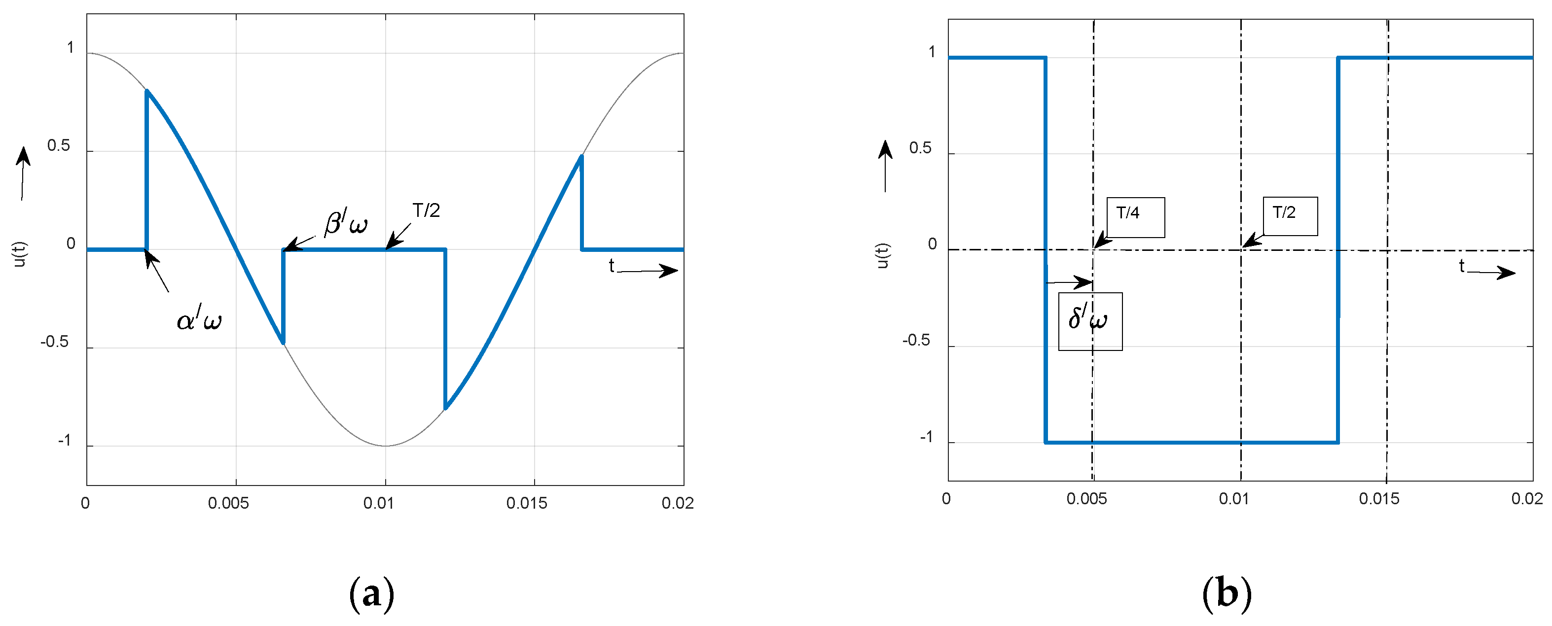
Fourier series are, in a certain sense, more universal than the familiar Taylor series in calculus because many discontinuous periodic functions that come up in applications can be developed in the Fourier series but do not have Taylor series expansions [4]. As an example, let’s introduce some pulse time waveforms generated by power electronic systems [5,6].
Fourier series is given by the relation, [1,2,3,4]
where are amplitudes of harmonic functions, which are the function of the Fourier coefficients , multiplicated by maximal value or [7]
where
Current waveform under linear R-L load can be derived using complex conjugate amplitudes [5] applied on Equation (4b) and zero initial conditions
where and .
Comparing amplitudes of component in (.) and we obtain
after substituting into , the relation for the steady state is obtained
The Equation (5d) thus represents the steady-state component of the current. In our case of rectangular supply voltage, (Figure 1b)
the transient component can be calculated easily because of first order system
where .
Then, the total transient time waveform of the load current will be
Note: In the case, when the system is the 2nd and higher order the transient component can be calculated using Laplace or Laplace-Carson transform (), respectively, when the notation of Equation (1a) is [7]
The last Equation (4) can be used later for the transient Fourier analysis, but it will be significantly simplified which is one of the goals of this paper.
Figure 1.
Time waveforms of non-harmonic courses used in EE generated by PES compensator (a) and inverter (b).
Figure 1.
Time waveforms of non-harmonic courses used in EE generated by PES compensator (a) and inverter (b).
- # Analytical solutions of transient using Fourier series using the Laplace-(Carson) transform and complex time vectors inside one period
Let´s suppose a single electrical R-L circuit supplied by harmonic voltage, Figure 2.
In case of harmonic sinusoidal supply, it is valid
where is a voltage connection angle to the load circuit or/and the initial angle of the time vector in the complex Gaussian plane.
Going back to the Fourier series, then using the relation we can write in complex domain
where time course of any-th harmonic of, e.g., the course in Figure 1b, while the angle frequency will be replaced by the frequency of -th harmonic , the phase displacement by , and by .
After decomposing as a sum of the first and higher harmonic components where the first term is a simple vector () starting at rotated by an angle , and the second one is the sum of the higher harmonic phasors .
It is simpler to sum these two current vectors in a coordinate system fixed to the fundamental of the voltage vector. In this rotary coordinate system, the fundamental current is stationary, and the path of the current harmonics is a closed loop.
Graphics interpretation in the Gauss plane is shown in Figure 3.
Going back to the transfer analysis, each harmonic component of the sum in Equation (6a) can be further processed using Laplace or Laplace-Carson transform. So, by transforming any harmonic given by Equation (5c) we get
using Laplace transform or
using Laplace-Carson transform.
Comparing Equations and we can see a considerable simplification of the notation.
- Then, since the operator impedance , and using Equation the complex time vector of the operator current gives
Applying inverse transform using Cauchy-Heaviside theorem
Then the relationship is obtained
By introducing complex impedance we get
and consequently, respecting the different switch-on angle
From this Equation (5c) holds for the real part
for or/and
for , respectively.
Supposing we can easily get the steady state for variable , such as
for .
Steady-state component is also - more easily - obtained using symbolic calculus and complex time vectors respectively, directly without transformation.
From where the real part is founded the time waveform of the fundamental current variable .
Time waveforms of the higher harmonics are similarly, while the angle frequency will be replaced by the frequency of -th harmonic , the phase displacement by , and by
That circumstances are graphically presented as sum of fundamental and higher harmonics in Figure 4.
- Respecting Equation (10b) and (10c) we can graphically image in the complex Gauss plane in Figure 5.
The course of higher harmonics in the range is shown separately in Figure 6a in both stationary and revolving coordinate system [6] and for the transformation of the vector of higher harmonics, the relation applies
Adding vectors of fundamental and higher harmonic components - similarly as in time domain – we get
Since the first term is a simple rotating vector (i.e., phasor) starting at rotated by an angle , the second one is the sum of the higher harmonic phasors .
The obtained result can be displayed, Figure 6.
Supposing equal 0 the steady-state is simply
where and thus the amplitude spectrum is monotonically decreasing. The fundamental harmonic in time domain is given by Equation (14b) if the switching angle δ were zero.
for .
The transient component one obtains from Equation for ‘cosine’ supply (with cosine components)
Or for ‘sine’ supply (with sine components).
Graphic imaging in the time domain is shown in Figure 7.
Using the above approach given by Equations (7a,b)–(11c), it is possible to calculate the current time course of any -th harmonic, thus
and its real part
So, the transient course will be
Graphic interpretation of Equation is shown in Figure 8.
Respecting Equations (15a) and (16) we can graphically image in the complex Gauss plane in Figure 9.
3. Transient Analysis of PES System using Fourier Integral Transform
As the Fourier transformation is defined over the entire time and not just for the positive values of time. However, in the circuit analysis, as was previously mentioned, the forcing functions and their responses are usually initiated at . Therefore, for such functions, the Fourier transform (Equation (4.13a)) might be written as
where means the unit-step function at .
Compared to the Laplace transform, for the function that does possess condition (Equation (4.39a)) we may find the Fourier transform by just replacing s with in the Laplace transform, i.e.,
This way of finding the function spectra for most of the non-periodic functions is the simplest and most convenient one.
In the next power electronics applications, we solve the transient analysis by both methods: firstly, using Fourier series/expansions focusing on the steady-steady operation, and then by Fourier transform focusing on the transient analysis.
- # Case of passive resistive-inductive load (without e.m.f.)
The connection of the electrical circuit is shown in Figure 10a, principle courses of the input and output (load) voltages in Figure 10b.
For AC symmetric waveform is valid
Fourier coefficients for -harmonics type of cosine
As then and
Since
And similarly for sine-coefficients
As then and
Since
Thus, the input voltage expressed by the Fourier series is defined using Equations .
Then, for the load current using Equations (18b) and (19)
where and .
Note: with a purely inductive load () the transient component will zero
Note: if and the load current will be purely sinusoidal one i.e., for fundamental harmonic
If the load current will be zero, then and so
from where it is possible to obtain the angle , e.g., in an iterative way. If it means that the load is purely inductive.
Graphic interpretation of Equatiom is shown in Figure 11. Parameters of the system are given in Table 1.
The solution of the transient phenomenon of the system is significant only in the case of uninterrupted current, with the turn-on angle equal to the phase shift angle, i.e., 36.76 – 90 = - 53.24 °el. Then the current will be pure sinusoidal. During the transient state by switching on at α = 0 the current will increase from zero to a steady state according to relation (6c) modified for the fundamental harmonic
The waveform for is shown in Figure 12.
Since the equation consists of steady- and transient-state components, we can write
Taking into account Tables 4.2 and 4.3 in [Sh] the Fourier transform of function can be derived (a simplified approach [Sh]) namely the time-shift rule
where .
Then, for steady-state component
And, for transient component
The graphic interpretation of the amplitude spectra of both components is shown in Figure 13 in the relative p.u. units (i.e., .
Since the time constant is rather small (2.3875 msec.), i.e., smaller than one-fourth of the time-period (Figure 12) the predominant component is the steady-state one.
# Case of active-inductive load with back e.m.f.
The connection of the electrical circuit is shown in Figure 14a, principle time waveforms of the input and output (load) voltages in Figure 14b, where the input voltage is harmonic cosine function, and S1 and S2 are electronic switches.
Fourier coefficients of that series are calculated by Euler relations.
If
Or
The same result we get using Equation for
Similarly for sine-coefficient of fundamental harmonic
Checking,
Fundamental harmonic rms value
Parameters of the system are given in Table 2.
# Transient analysis using Fourier transform (and under decreasing cosine function)
Supposing exponentially increasing back emf voltage (e.g., start-up of electric motor) and constant harmonic input voltage then the voltage on the load (inductor) will be decreasing cosine function
where respects a rise of the back-emf voltage, Figure 17a (green). If we take according to (28) the corresponding load current of the inductor can be calculated, in Figure 17b (red).
Applying the Fourier transform on the transient voltage we can write [1]
where represents a damping of the circuit and is an angular frequency of the input voltage.
The infinitive integral can be calculated substitution or per partes rules with the result
with use of the Euler formula as a substitution for .
So, after the establishment of integration boundaries
thus
The magnitude spectrum of
The graphic interpretation of the magnitude spectra of is shown in Figure 18 in the relative p.u. units (i.e., .
The phase spectrum of we can calculate as an arctan function of the share quotient of the imaginary and real part of the magnitude spectrum ()
Similarly, as for - if we admit that load current is decreasing quasi sinusoidal function (Figure 17b) - we can apply its Fourier transform
where the maximal value of the load current
and where as mentioned above.
The magnitude spectrum of the current Fourier transform is depicted in Figure 19.
4. Discussion and Conclusions
It is evidently from the Figure 13b, Figure 18 and Figure 19 that during the transient state both quantities show a continuous spectrum of harmonic components, including the fundamentals. It means that electric power as a product of current and voltage, it will also contain a distortion component despite being a harmonic network and a linear load (resistive or inductive, or both). Although slightly strange it is one of the important contributions to practical applications.
Although classical Fourier analysis with specifically Fourier analysis, are not particularly suitable for transient signal analysis compared to other analysis, after all, they also bring certain advantages. It is primarily:
- -
- knowledge of the content of harmonics in the investigated course,
- -
- resulting easy calculation of the harmonic distortion of the signal [10],
- -
- the investigated function does not necessarily have to be analytical in the scope of the period, and can be specified e.g., as a look-up table.
In combination with Laplace, or Laplace-Carson transform can also be used in Fourier analysis to solve transient phenomena particularly when solving the steady states within one time-period.
The article shows two new effective approaches for solving transient analysis and that:
- -
- -
That transformation with its magnitude and phase frequency spectra which cannot be obtained by other known transformations [11].
In conclusion, this paper presents a significant advancement in transient Fourier analysis, offering novel insights into the behavior of single harmonics and their superposition in dynamic systems. The utilization of complex time domain analysis and the innovative techniques employed herein hold great promise for further advancements in this domain.
Author Contributions
conceptualization, methodology, supervision by B D.; formal analysis, data curation, investigation, validation by J.Š.; software, visualization by R.K.; resources, original draft preparation, review and editing by M.B.; and project administration, funding acquisition by M.P. All authors have read and agreed to the published version of the manuscript.
Funding
This research was funded by the Slovak Research and Development Agency, Bratislava, Slovakia, grant number APVV-22-0330 and the APC was funded by the Scientific Grant Agency of the Slovak Republic, Bratislava, Slovakia, grant number VEGA 1/0314/24.
Data Availability Statement
Not available.
Acknowledgments
This research was also supported by the University of Žilina, UNIZA Grant Project: “Research of methods for investigation of operating and fault conditions of drives with multiphase asynchronous motor.”.
Conflicts of Interest
The authors declare no conflict of interest.
Appendix A
It will be supplemented if necessary.
Appendix B
It will be supplemented if necessary.
References
- Shenkman, A.L. Transient analysis using the Fourier transform. Transient Analysis of Electric Power Circuits Handbook. Springer, Dordrecht, The Netherlands (NL), 2005, Chap. 4, pp. 213-263, ISBN-10 0-387-28799-X (e-book). [CrossRef]
- Bai, H.; Mi C. Transients of Modern Power Electronics. 2011, John Wiley & Sons, Ltd., Print ISBN: 978-0-470-68664-5, Chichester, UK.
- Beerends, R.J.; Morsche, H.G.; Berg, J.C.; Vrie, E.M. Fourier and Laplace transforms, Publisher: Cambridge University Press, 2003, Part 4, pp. 267-330.
- Kreyszig, E. Kreyszig; Kreyszig, H;.Norminton, E.J. Advanced Engineering Mathematics. John Wiley & Sons, Inc., New York, USA, 2011, Chap. 6, pp. 203-255, ISBN 978-0-470-45836-5.
- Takeuchi, T.J. Theory of SCR circuit and application to motor control (in Russian). Energy (Энергия) Publisher, Moscow–Leningrad (St. Petersburg) division, 1973, 248 pgs., IDC- international decimal classification: 621.313.13-53. 621.314.632.
- Mohan, N.; Undeland, T.M.; Robbins, W.P. Power Electronics: Converters, Applications, and Design. Third Edition. John Wiley & Sons, Inc., New York, USA, 2003.
- Aramovich, J.G.; Lunts, G.L.; Elsgolts, L.C. Complex variable functions, Operator calculus, Theory of stability (in Slovak). ALFA Publisher, Bratislava, SK, 1973, Chap. 7, pp. 157-228.
- Oršanský, P. Complex variable theory (in Slovak). Textbook UNIZA, Žilina, SK, 2020, ISBN 978-80-554-1764-6.
- Smith, S.W.: The Complex Fourier Transform. Chapter 31 in: The Scientist and Engineer’s Guide to Digital Signal Processing. California Technical Publishing, 1997-2007, pp. 567-580, ISBN 0-9660176-3-3.
- Blagouchine, I.V.; Moreau, E. Analytic method for the computation of the total harmonic distortion by the Cauchy method of residues. IEEE Trans. on Comm., 2011, Vol. 59, pp. 2478–2491.
- Choi, M.-J.; Park, I.-H. Transient analysis of magneto-dynamic systems using Fourier transform and frequency sensitivity. IEEE Transactions on Magnetics, vol. 35, no. 3, pp. 1155-1158, May 1999. [CrossRef]
Figure 2.
Time waveform of considered voltage (a), and electrical circuit (b).
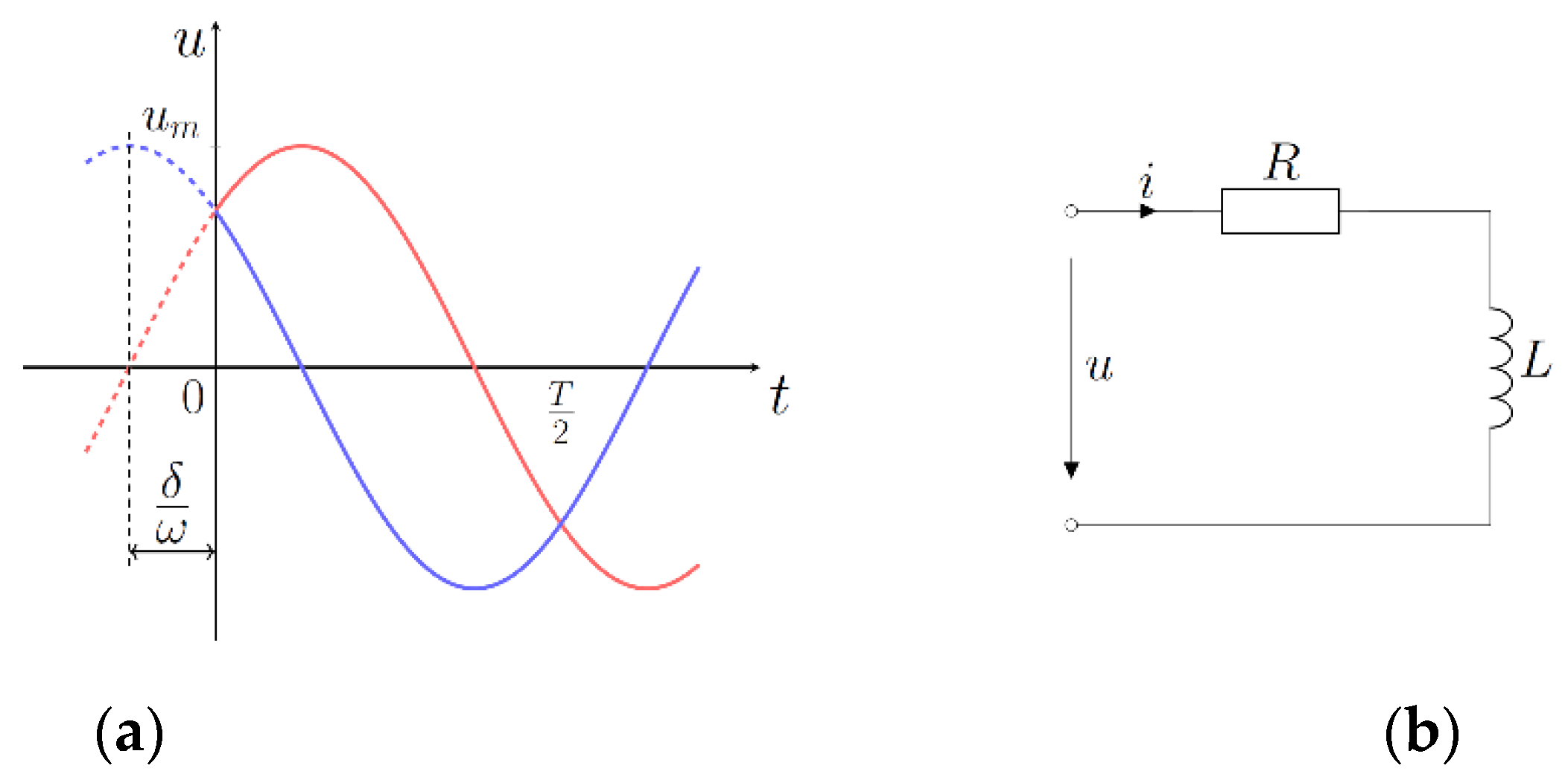
Figure 3.
Principle graphic representation of considered vectors in complex domain.
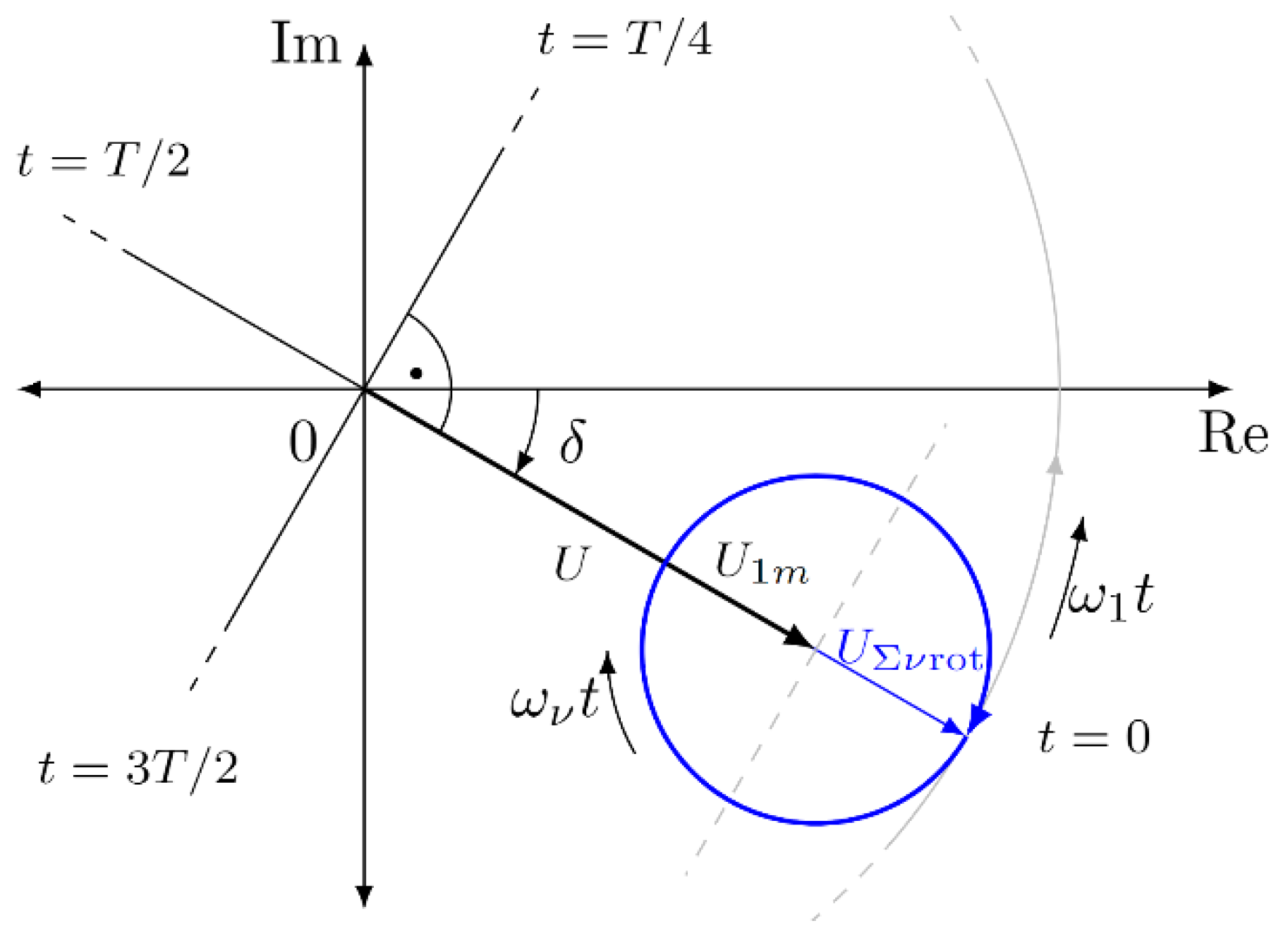
Figure 4.
Steady-state total current waveform decomposed into fundamental and sum of higher harmonics under different instant of switch-on: (a) and (b).
Figure 4.
Steady-state total current waveform decomposed into fundamental and sum of higher harmonics under different instant of switch-on: (a) and (b).
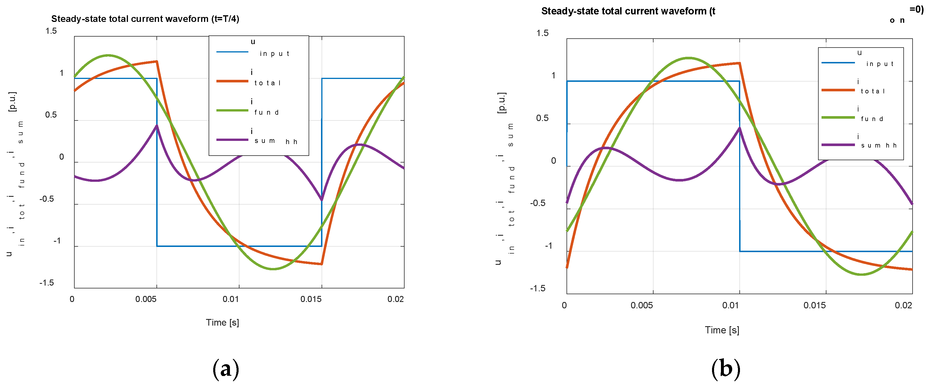
Figure 5.
Steady-state total current waveform decomposed into fundamental and sum of higher harmonics in complex domain.
Figure 5.
Steady-state total current waveform decomposed into fundamental and sum of higher harmonics in complex domain.
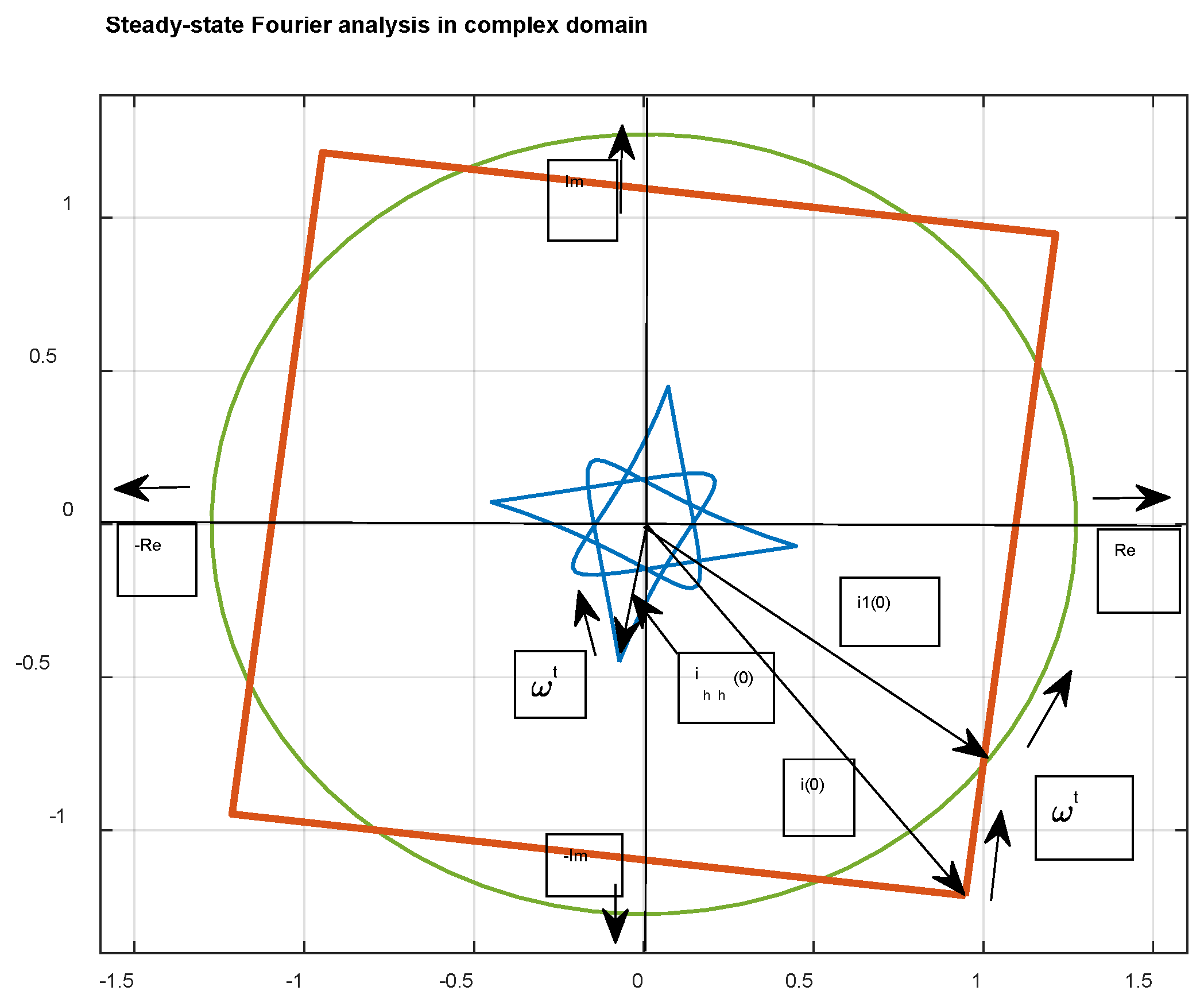
Figure 6.
Course of higher harmonics in the range (a), course both in stationary and rotary coordinate system (b).
Figure 6.
Course of higher harmonics in the range (a), course both in stationary and rotary coordinate system (b).
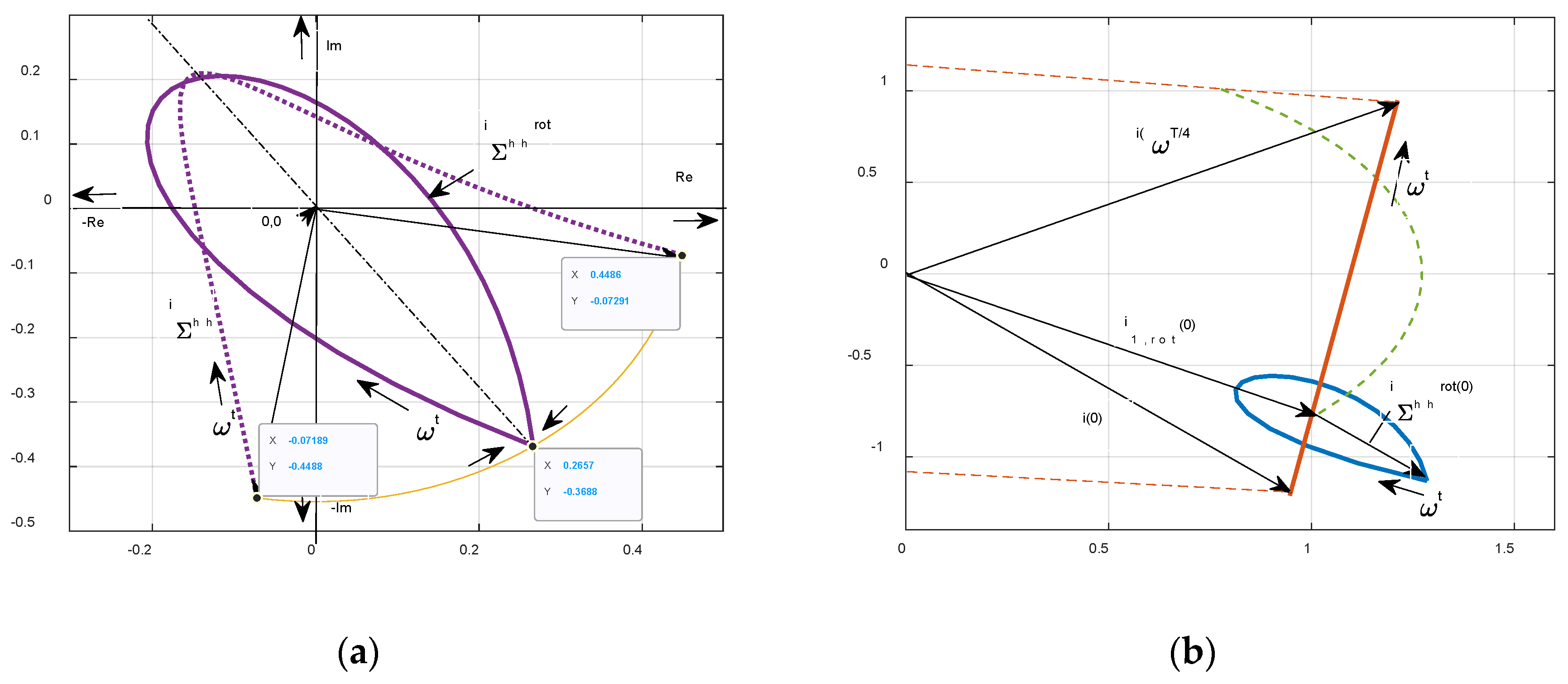
Figure 7.
Transient, steady-state and total components of current waveform.
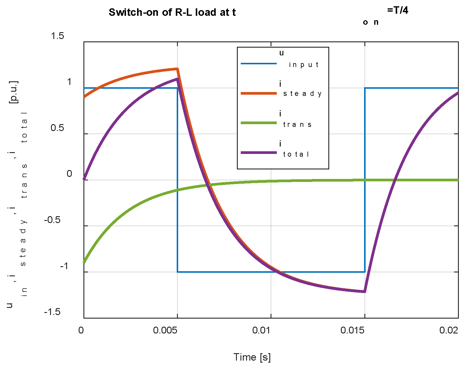
Figure 8.
Time waveform of the transient Fourier analysis in time domain at (a) and (b).
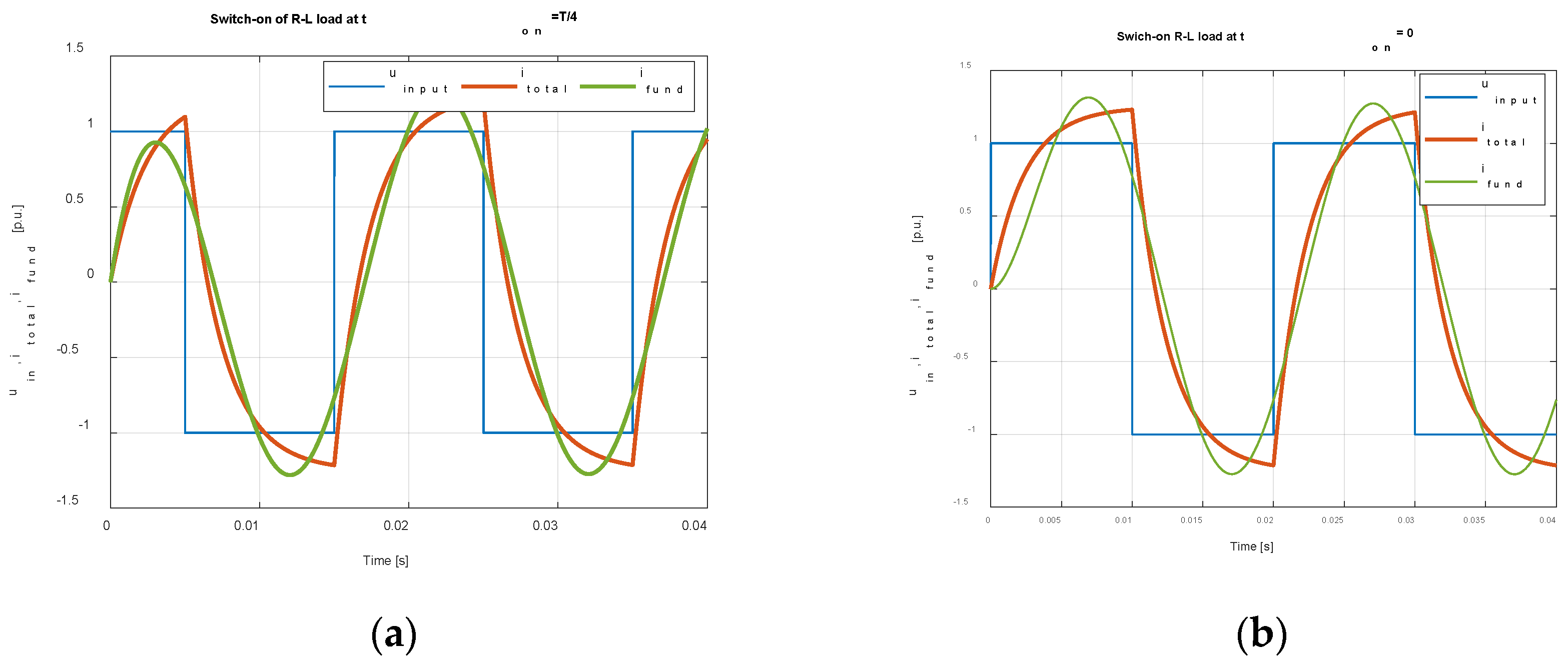
Figure 9.
Time waveforms of the transient Fourier analysis in the complex domain.
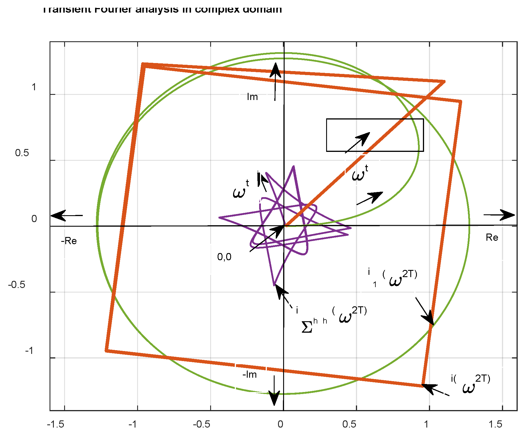
Figure 10.
Schematics (a) and courses of network and load voltages (b).
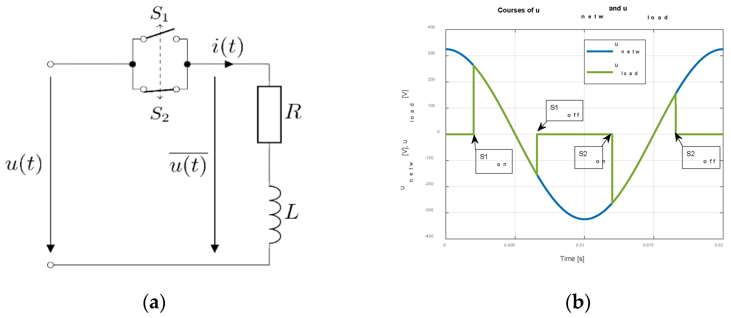
Figure 11.
Time waveform of the load current and load and network voltages (a), decomposition of the total current (b).
Figure 11.
Time waveform of the load current and load and network voltages (a), decomposition of the total current (b).
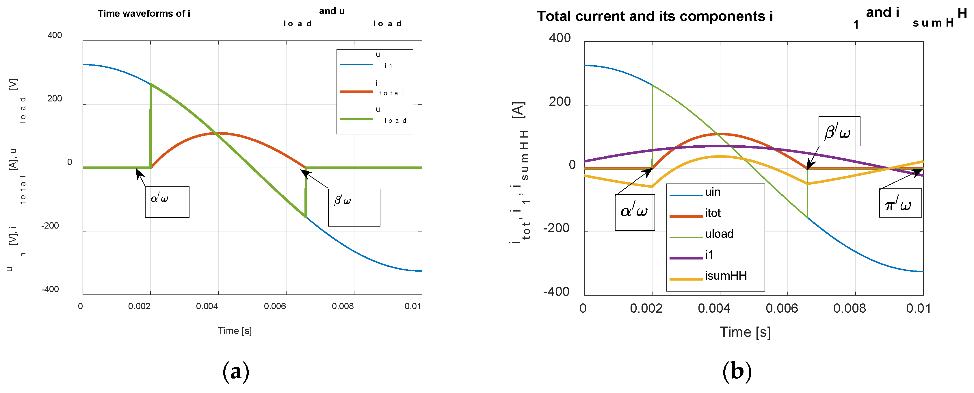
Figure 12.
Time waveforms of input voltage and load current.
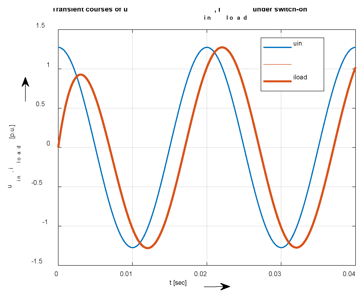
Figure 13.
Amplitude spectra of steady-state (a) and transient component (b) under - load in transient phenomenon at switch-on the system.
Figure 13.
Amplitude spectra of steady-state (a) and transient component (b) under - load in transient phenomenon at switch-on the system.
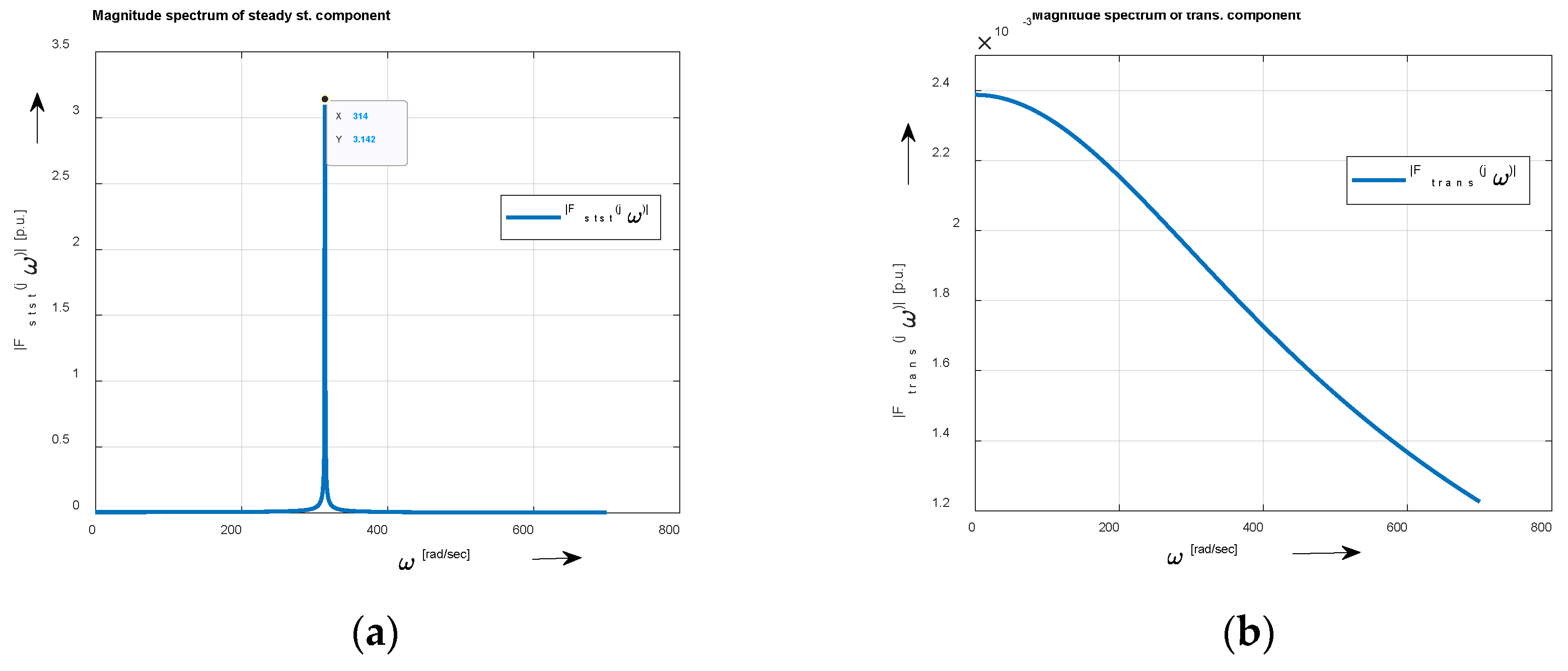
Figure 14.
Schematics (a) and courses of network and load voltages (b).
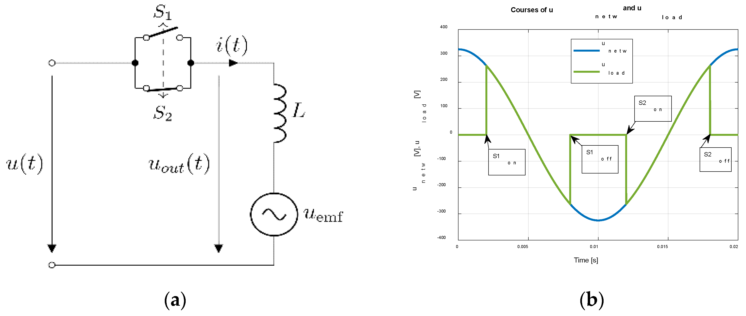
Figure 15.
Time waveform of the load current and load and network voltages (a), decomposition of the total current (b).
Figure 15.
Time waveform of the load current and load and network voltages (a), decomposition of the total current (b).
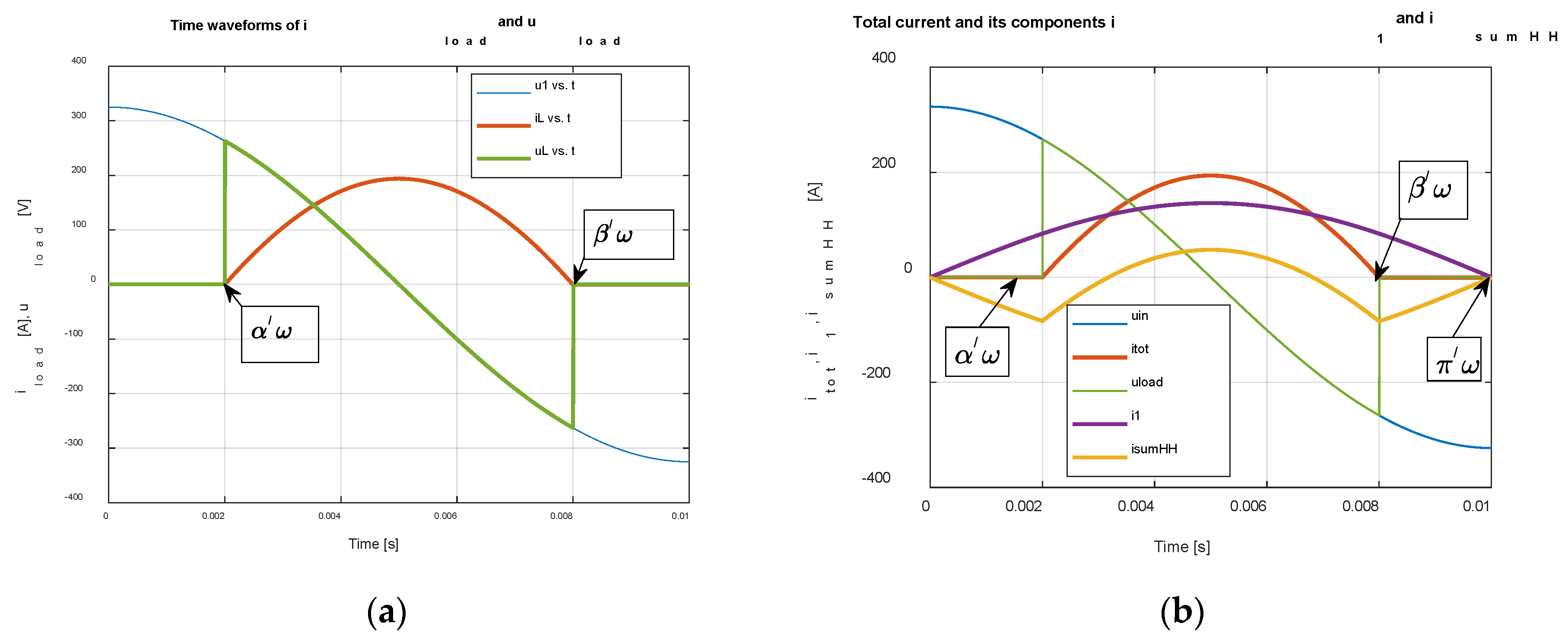
Figure 16.
Time waveform of the load current and load and network voltages under different magnitude of Uemf.
Figure 16.
Time waveform of the load current and load and network voltages under different magnitude of Uemf.
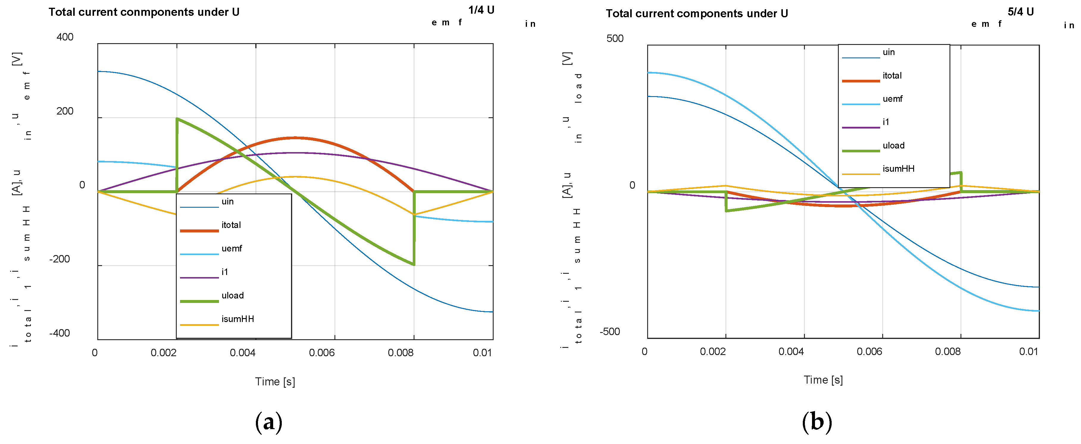
Figure 17.
Created a decreasing cosine function of the load voltage (a) and current (b).
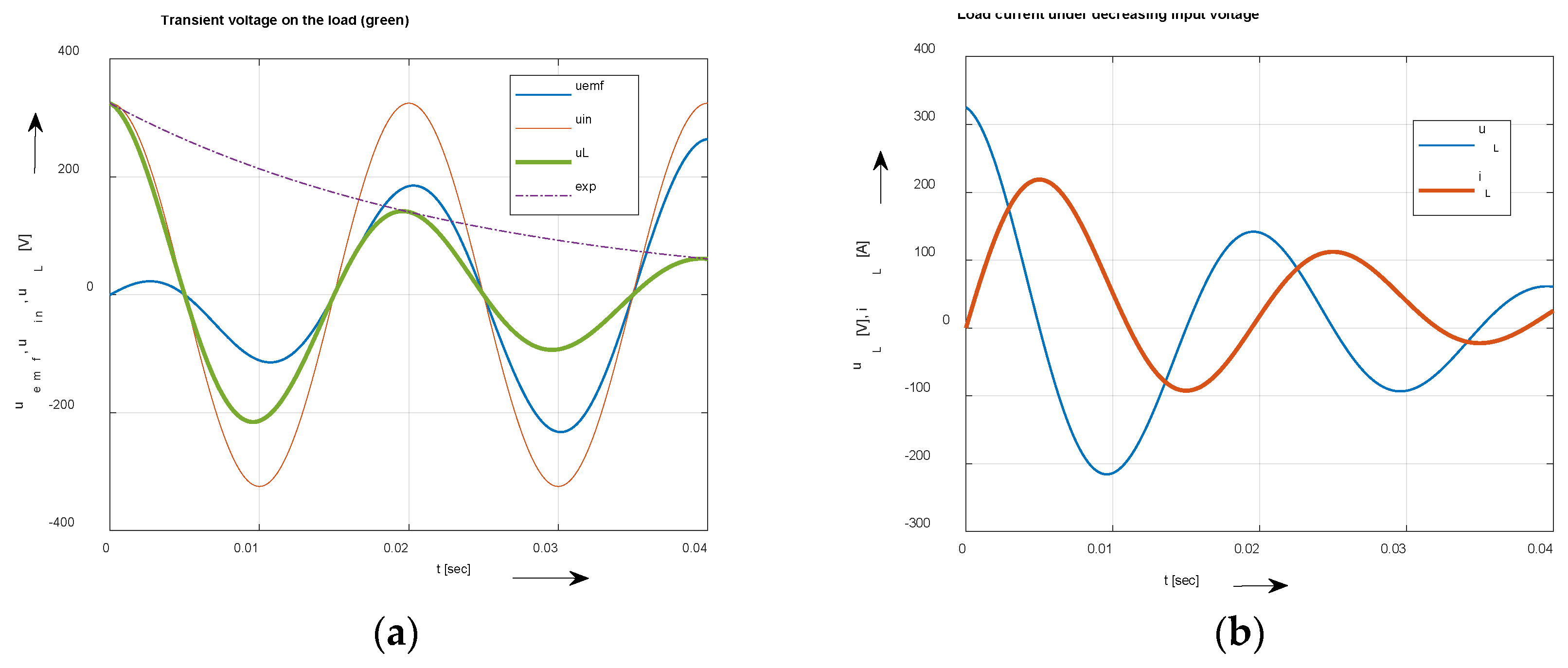
Figure 18.
A decreasing cosine function and its magnitude spectrum .
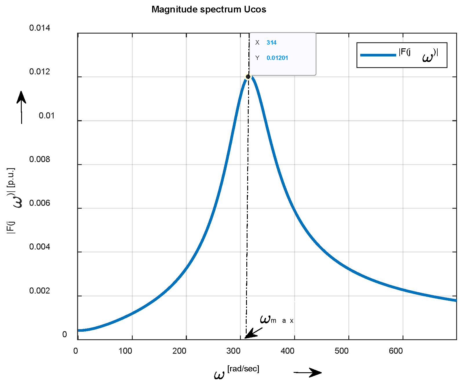
Figure 19.
Magnitude spectrum of the decreasing sinusoidal function.
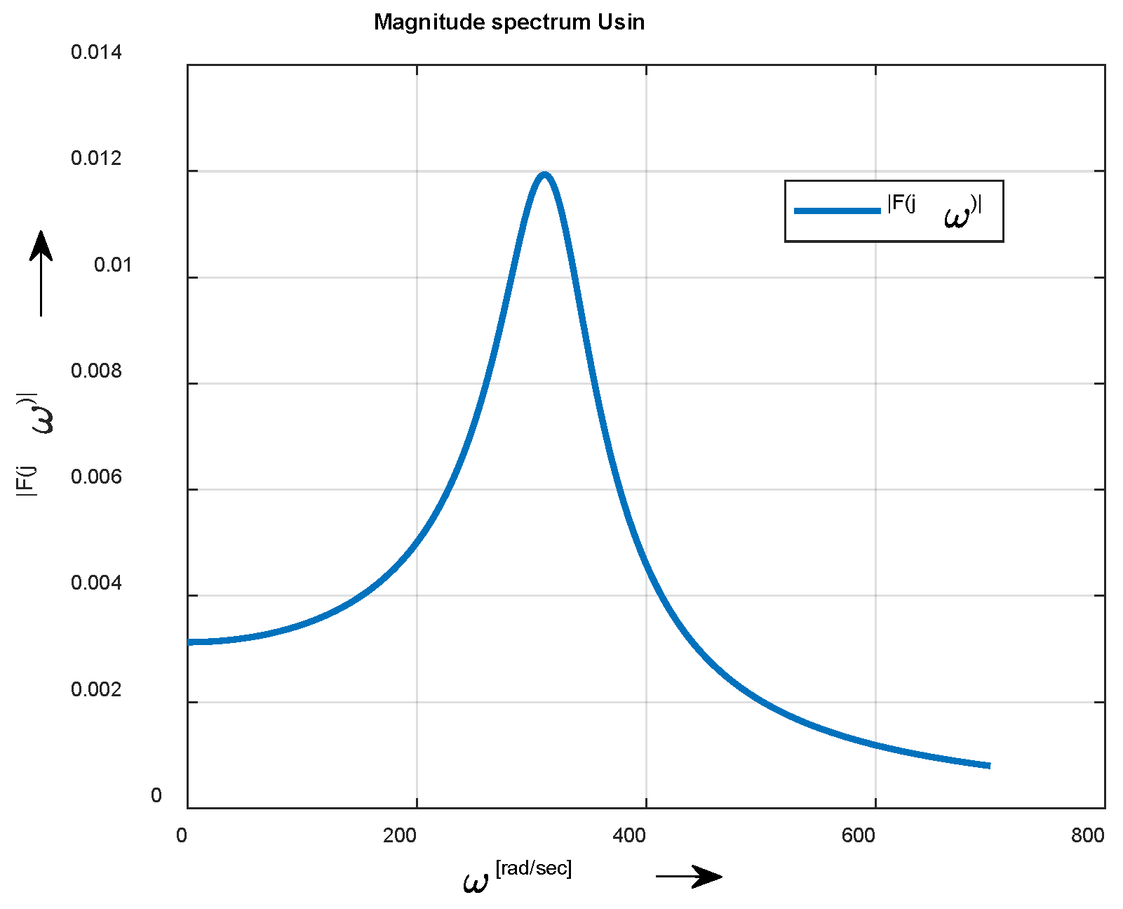

Table 1.
Parameters of the system.
| Um [V] |
[Hz] |
R [Ω] |
L [mH] |
Z [Ω] |
[ms] |
[deg] |
|---|---|---|---|---|---|---|
| 325 | 50 | 18.4 | 43.93 | 23 | 2.3875 | 36.76 |
Table 2.
Parameters of the system .
| Um [V] |
[Hz] |
R [Ω] |
L [mH] |
Z [Ω] |
[ms] |
[deg] |
|---|---|---|---|---|---|---|
| 325 | 50 | 18.4 | 43.93 | 23 | 10 | 90 |
Disclaimer/Publisher’s Note: The statements, opinions and data contained in all publications are solely those of the individual author(s) and contributor(s) and not of MDPI and/or the editor(s). MDPI and/or the editor(s) disclaim responsibility for any injury to people or property resulting from any ideas, methods, instructions or products referred to in the content. |
© 2024 by the authors. Licensee MDPI, Basel, Switzerland. This article is an open access article distributed under the terms and conditions of the Creative Commons Attribution (CC BY) license (http://creativecommons.org/licenses/by/4.0/).
Copyright: This open access article is published under a Creative Commons CC BY 4.0 license, which permit the free download, distribution, and reuse, provided that the author and preprint are cited in any reuse.


