1. Introduction

Figure 1. The block diagram of the process-based digital twin based on the proposed data-driven processed-based fish feeding model.

Figure 1. The block diagram of the process-based digital twin based on the proposed data-driven processed-based fish feeding model.

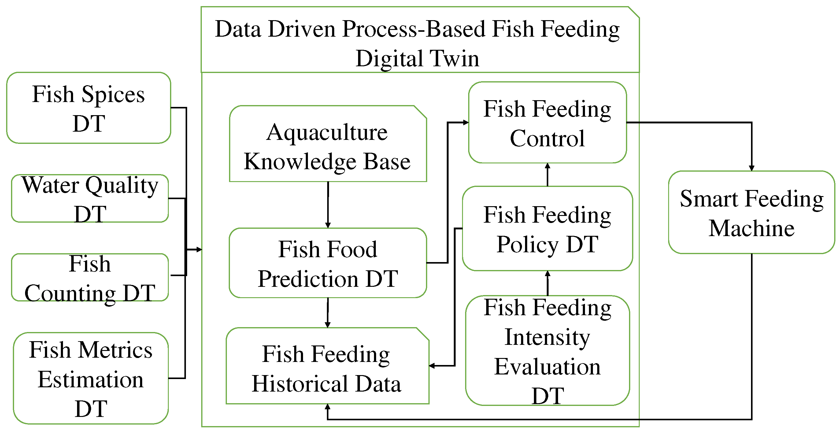
• Fish Species Input: This input specifies the type of fish to be bred and retrieves a set of genetic parameters from the aquaculture knowledge base. These parameters characterize the fish's growth model and are determined by genetics, independent of environmental factors. Initially defined by aquaculture experts, these parameters are subject to calibration and refinement through machine learning algorithms using historical fish feeding input and output data.
• Environment Input: The environment input comprises a set of continuously collected environmental data, including temperature, water velocity, dissolved oxygen, salinity, etc. These data are acquired using the deployed water quality DT object.
• Fish Metrics Input: This input consists of fish monitoring results, including current fish count, length, width, and weight, obtained through pre-trained deep learning prediction models analyzing data from RGB-D cameras or sonar imaging devices. The related DT objects encompass fish counting DT and fish metrics estimation DT.
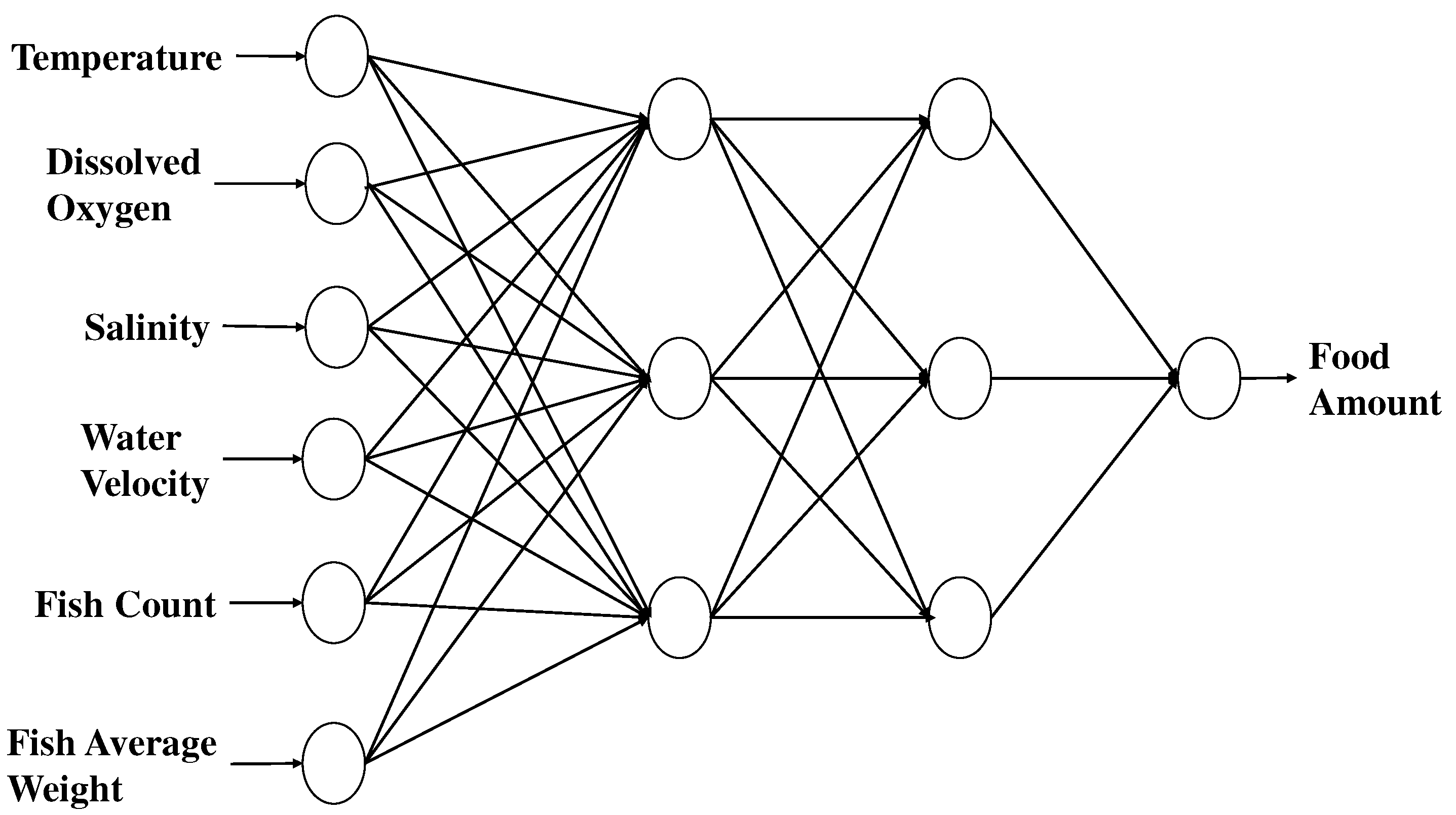
• Fish Food Prediction Model: An artificial intelligence neural network predicts the quantity of food to be dispensed into the fish cages, following our fish feeding policy, using remotely controllable smart feeding machines. This model is incorporated into the fish food prediction DT, which takes inputs from the water quality DT, fish counting DT, and fish metrics estimation DT to determine the daily fish feeding amount.
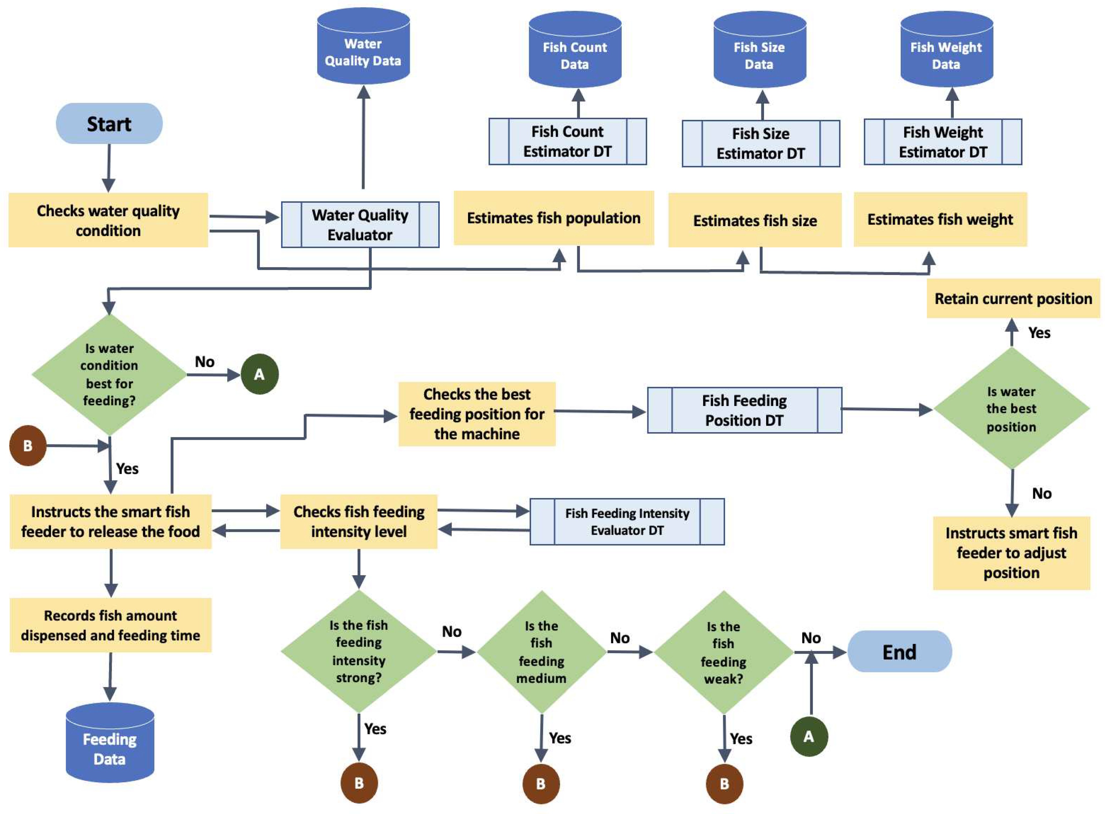
• Fish Feeding Intensity Evaluation DT: This deep learning model predicts the level of fish feeding intensity, which is then used as input for the fish feeding policy DT to regulate the optimal actions controlling the smart feeding machine and minimize potential residual food during daily fish feeding.

2. Materials and Methods

2.1. Cloud-Based Digital Twin Architecture

Figure 2. Cloud-based digital twin system for fish feeding management.

Figure 2. Cloud-based digital twin system for fish feeding management.

This section provides an in-depth look into our digital twin architecture and its various components essential for achieving optimal fish feeding management, as illustrated in Figure 2. Our architecture comprises three major components.

Initially, we employ physical devices equipped with sensors and a smart feeding machine featuring remotely controllable actuators. These sensors autonomously collect and transmit data, including fish images and water quality information, from the farm environment to the cloud system, forming the second component. The on-site remote feeding machine facilitates automated feeding control. To enable the deployment of IoT devices in the aquaculture setting for continuous data collection, our sensors and actuators are equipped with Wi-Fi or 4G/5G telecommunication capabilities for wireless data transmission.

The cloud system is further divided into two distinct components: data management services and the fish feeding digital twin. Data management services integrate a database management system to securely store, organize, and manage data collected from the aquaculture farm. Simultaneously, the application server serves as a middleware platform for running applications related to digital twin services, while the web server offers services accessible via the web.

In the realm of fish feeding management, the digital twin relies on the proposed data-driven, process-based fish feeding model, encompassing two significant services: fish metrics estimation and fish feeding. These services leverage deep learning models for their implementation, alongside feeding policy optimization through Q-Learning. Further details regarding the fish feeding management model will be elaborated upon in subsequent sections.

2.2. The Digital Twin for Fish Feeding Management

The first step to construct the digital twin for fish feeding management is to understand the aquaculture processes to operate a fish farm. The first step of the cage culturing is the development of net cages for fish breeding. As shown in Figure 3, in this study, the net cages for experiments are in the offshore Pingtung and Penghu, Taiwan. The circular perimeter of inner pipe of the former is 102 meters, which is a large submersible cage; on the contrary, the net cages in Pinghu are relatively small and divided into types: the circular cage with the perimeter of inner pipe of the former to be about 30 meters; the squared cage of 10x10x8 m3 in size. The cages in Pingtung are at open sea areas which have deeper waters and stronger ocean currents, and thus could prevent environmental pollution and fish diseases. The tested offshore net cage in Pingtung would have annual output of the cultured snubnose pompano up to 200 tons/cage year. However, the risk and the operation cost of the aquaculture with large offshore net cages are relatively high as compared with small net cages in Penghu. Thus, the sensors and the automatic machines of IoT systems should be different for different environments to facilitate the farmer to operate aquaculture processes.

Studying fish growth models is crucial in the context of aquaculture processes. Fish growth, defined as the change in body mass over time, results from the interplay of two opposing processes – one that increases body mass and another that decreases it. This growth phenomenon is intricately linked to weight and time, allowing growth data to be constructed directly or indirectly using these parameters [29]. From an energetic perspective, Ursin's model [30] characterizes fish growth as the difference between anabolism (the building-up phase) and catabolism (the breakdown phase). This energetic concept is reflected in the energy budget presented in Figure 8, and Ursin's bioenergetic model can be expressed as

$$\frac{dW}{dt}=H{W_t}^d-k_{cata}{W_t}^n$$

(1)

where $W_t$ represents the weight of the fish at time t, $H{W_t}^d$ is the energy absorbed in the entire anabolism, and $H$ and $d$ represent the anabolism coefficient and slope related to anabolism and fish weight, respectively. On the other hand, $k_{cata}{W_t}^n$ is the energy lost in the whole catabolism where $k_{cata}$ and $n$ is the catabolism coefficient and the slope related to the catabolism and fish weight, respectively. Yang [31] defined the detailed fish growth model derived from Ursin’ model and took into account the effect of environmental factors such as growth and water quality. The model includes the effects of different parameters such as water temperature (T), body size and weight (w), un-ionized ammonia (UIA), dissolved oxygen (DO), photoperiod (p), and relative feeding ratio (f). Thus, the growth rate model of a fish is again described as the difference between anabolism and catabolism:

$$\frac{dW}{dt} =\underset{\mathrm{anabolism}}{\underbrace{\varnothing \left(p,f,T,DO\right)\nu \left(UIA\right)}}{w}^m - \underset{\mathrm{catabolism}}{\underbrace{k\left(T\right)}} w^n$$

(2)

where $\varnothing \left(f,T,DO\right)$ (g^{1− m}day^{− 1} ) and $\nu \left(UIA\right)$ are the coefficients of anabolism; m is the exponent of body weight for net anabolism; k(T) (g^{1− n} day^{− 1} ) is the coefficient of fasting catabolism; n is the exponent of body weight for fasting catabolism. Although more factors should be considered to realize the fish growth model, Equation (2) lists the most important factors to measure the fish growth rate. In [32], based on (2), Chahid et al. proposed a Fish growth trajectory tracking using Q-learning [33] to determine a fish feeding policy which achieves 1.7% and 6.6% relative trajectory tracking errors of the average total weight of Nile Tilapia (O. niloticus) from both tanks on land and floating cages, respectively.

Figure 4. The wireless communication based AIoT system for automatic data collection from net cages, which are further inputted to our digital twins for performing intelligent fish feeding control.

Figure 4. The wireless communication based AIoT system for automatic data collection from net cages, which are further inputted to our digital twins for performing intelligent fish feeding control.

The fish model mentioned in (2) was initially developed within the context of a semi-intensive aquaculture pond to determine the nutrient requirements for Nile tilapia [31]. This implies that in such a setting, fish growth and production are partially controlled, with aquatic species' growth relying on a combination of natural feeds and aquafeeds. It is evident that the mathematical fish model can be adapted for net cage culturing by substituting the parameters specific to Nile tilapia with those corresponding to the target aquatic species [34]. By incorporating a knowledge base pertaining to the target aquatic species to define the parameters in the growth model, we can create a synthetic training dataset that accounts for the uncertainties and measurement noise present in real aquaculture environments. This dataset is then utilized to train a transformer-based deep learning model [35], which predicts fish growth rates based on environmental factors and feeding.

Furthermore, the fish growth model is fine-tuned by incorporating test data obtained from our experimental net cages using the deployed IoT sensors. While this approach is one possible way to design our fish feeding Digital Twin (DT) object, it remains somewhat detached from real-world aquaculture processes. In this study, we aim to design our DT architecture based on the physical processes, as defined by aquaculture experts, using a simplified version of (2).

Figure 4 illustrates the proposed AIoT architecture, which collects water quality data, optical stereo RGB videos, and sonar images from our experimental net cages. The digital twin is deployed on our cloud servers. In practice, as depicted in Figure 5, the hardware architecture of the proposed data collection system is further divided into three distinct sub-systems. These include an AI buoy for water quality inspection, as well as two lightweight broadband carriers for operating optical stereo cameras and sonar image cameras, respectively. Our AI buoy system primarily consists of a solar panel, a control box, two lifebuoys, a steel skeleton, and sensors for collecting data on water flow, temperature (T), dissolved oxygen (DO), and salinity. Additionally, three server-side AI programs are also established on the shore server within the cloud [13].

For each data collection sub-system, we have implemented sonar panels to recharge the battery set, ensuring a continuous power supply to operate the sensors, wireless base station, and communication hub. As a result, these systems achieve the goal of promoting environmental, social, and government (ESG) standards without introducing any additional carbon footprint in fish production.

Figure 5. The hardware architecture of the proposed data collection system is divided into three different sub-systems: (a) the AI buoy for water quality prediction; (b) the lightweight broadband carrier for operating optical stereo camera; (c) the lightweight broadband carrier for operating sonar image camera.

Figure 5. The hardware architecture of the proposed data collection system is divided into three different sub-systems: (a) the AI buoy for water quality prediction; (b) the lightweight broadband carrier for operating optical stereo camera; (c) the lightweight broadband carrier for operating sonar image camera.

Figure 6. The sequence diagram of the underwater video surveillance system for fish metrics estimation.

Figure 6. The sequence diagram of the underwater video surveillance system for fish metrics estimation.

During the daily fish feeding process, our two-mode underwater video surveillance system is activated to capture surveillance videos, which are then automatically transmitted to the cloud for fish metrics estimation using our broadband wireless communication system. Additionally, a software daemon is implemented in the cloud to monitor incoming surveillance videos, storing them into the network-attached storage (NAS), and activating pre-trained deep learning models for fish count, length, and weight estimation [17,21]. Figure 6 illustrates the sequence diagram of the underwater video surveillance system, which provides fish metrics data to the digital twin for further decision-making in fish feeding management. Figure 7 showcases the fish metrics estimation models that were proposed in our previous work [17]. Instead of introducing new deep learning models to complete the AI functions of the fish metrics estimation Digital Twin (DT) object, our current study focuses on integrating mature prediction models into our DT objects. It is worth noting that the performance of prediction models can be enhanced by replacing them with new state-of-the-art models. The cloud infrastructure supports a server-side maintenance scheme, offering plug-in services to front-end users. Consequently, our DT objects are autonomous and possess self-learning capabilities, making them adaptable and evolvable.

Figure 7. The stereo image based fish metrics estimation model proposed in our previous work [17].

Figure 7. The stereo image based fish metrics estimation model proposed in our previous work [17].

Figure 8. The MLP based regression model for fish food prediction.

Figure 8. The MLP based regression model for fish food prediction.

The next step of our digital twin approach is to estimate the amount of food for the diary fish feeding. At time t, conventional fish farm determines the amount of fish food F_t for daily feeding process by the following equation:

$$F_t=k_t\times n_t\times {\overline{w}}_t$$

(3)

where $k_t$ is the relative feeding rate, $n_t$ is the number of fish and ${\overline{w}}_t$ is the average fish weight. In practice, the value of $k_t$ is set to be about 0.3 when the fish are kept on a well-controlled fish pond; however, it’s value is obviously dependent on the actual environmental factors. For example, the low temperature would decrease the appetite of fish and thus the resulting value of $k_t$ should be decreased to reduce the food residual. Actually, we cannot find a complete model to determine the optimal value of $k_t$ in the literature. Instead of using a function to determine $k_t$, we adopt a data-driven approach to predict the daily amount of fish food using an artificial neural network (ANN) regression model, which is a simple regression model with multi-layer perceptron (MLP) [36]. As shown in Figure 8, the inputs to the food prediction model include water quality data and fish metrics estimation results, e.g., the fish count and average weight; the output is the predicted food amount. A training dataset of about 200 records is collected from real fish farms are used to train the model. The testing accuracy is up to 98%. The fish food prediction DT is thus designed to predict fish food amount based on the human being experiences.

Figure 9. Flowchart of fish feeding procedure.

Figure 9. Flowchart of fish feeding procedure.

To carry out the fish feeding process, the predicted amount of fish food is dispensed into the food bucket of our intelligent feeding machine. Figure 9 provides a flowchart depicting the fish feeding procedure, which operates during actual feeding times. It collaborates with various digital twin (DT) objects, integrating multifunctional AI capabilities, thus rendering the framework versatile for feeding management. We have integrated six DT objects deployed within the AI-empowered cloud to oversee fish feeding activities alongside the smart fish feeder machine.

Initially, the suitability of water quality conditions for feeding is assessed. The Water Quality DT is then invoked to evaluate the current water quality condition and provides feedback, which serves as the basis for initiating feeding. Once water quality approval is obtained, the smart feeding machine is controlled to release the initial batch of fish food. Additionally, other DT objects, such as the Fish Count Estimator, Fish Size Estimator, and Fish Weight Estimator, perform their respective AI functions as indicated by their names. All estimations generated by these three DTs are stored in the cloud's database for further data analytics, including growth predictions and optimizations.

As the water quality condition meets the criteria, the smart feeder dispenses an initial amount of bait. When the fish are released from the smart feeder machine, they retrieve the food from the water's surface, resulting in visible water splashes that become more pronounced as feeding progresses. Leveraging fish feeding behavior, the area with significant surface motion determines the current position of the fish within the cage. To ensure accurate food placement, we have integrated a Fish Feeding Position DT, which detects the current feeding area or zone and adjusts the smart feeder's gun barrel position based on the estimated feeding location. This optimization ensures that the feeder dispenses feed at the current feeding spot.

Additionally, the smart fish feeder is equipped with actuators for control and can receive information to assist with feeding, such as determining the feeding amount. Another DT object, known as the Fish Feeding Intensity Evaluator [12], is employed to assess the fish's feeding intensity, categorized into four levels: strong, medium, weak, and normal. As the feeding intensity decreases from strong to weak, the amount of feed dispensed is reduced. When the observed fish feeding intensity reaches none, feeding ceases. The total feeding amount is also monitored and stored in the database, along with fish count information and average weight.

To minimize food wastage, the predicted food amount F_t is divided into n parts for fish feeding when we specify n intervals to complete the daily feeding process using the smart feeding machine. Essentially, for each part, our fish feeding control module issues a command to the feeding machine to dispense the quantity of food F_t⁄n into the target cage for fish feeding. However, this approach can lead to a high probability of food wastage when the current fish feeding intensity level is normal or weak. To address this challenge, we employ a Markov decision process (MDP) to model the decision-making process regarding the amount of fish food to be used for each part of the feeding. The MDP model for fish feeding management comprises the following components.

State: S is a set of finite states that describes the status of the fish feeding process. It contains two parameters i and $v_j$ to describe the part number and the accumulative amount of food, respectively. For the daily feeding time t, the values of $v_j$ and i are limited by the predicted food amount $F_t$ and the number of parts n, respectively. In other words, the states define the possible responses of the fish feeding machine to the possible input actions. To simplify the state set defined as $S=\left\{s_{0,0},s_{0,1},\dots ,s_{n-1,m-1}\right\}$ of MDP as a lookup table, we discretize the continuous parameter $v_j$ into m levels, which define the accumulative amount of food, i.e., $v_j=\left(j+1\right)F_t/m$. The finite set S with the state is defined as the pair (food amount, part number).

Action: $a\in \mathrm{A}=\left\{f,e\right\}$ is a set of possible control actions which activate the feeding machine to send relative feeding rate f of the schedule food at state s. To simplify the control of our feeding machine, the relative feeding rate is quantized into two levels, i.e., 0 and 1, corresponding to two operation modes, i.e., to turn on and to turn off the feeding machine, for sending the scheduled food amount $F_t/m$ and zero food into the cage, respectively. On the contrary, the parameter e, i.e., the food eaten ratio, is quantized into 4 levels corresponding to the four fish feeding intensity levels, i.e., ‘Strong’, ‘Medium’, ‘Weak’ and ‘Normal’. In practice, the setting of e is based on the predicted results of the fish feeding intensity evaluation DT. For each action a, the MDP model will result in a state transition.

Reward: r(s,s′) is reward received after transitioning from state s to state s′ , after applying the action a. In this work, the optimal Q-learning policy based on MDP tracks a desired fish feeding trajectory while penalizing the food eaten ratio (e) for aquaculture cages. We formulate the reward function r(s,a) for offshore cages as a regularized trajectory tracking error and food eaten ratio as follows:

$$r_i\left(s_{i,j},a_i\right)={f_{a_i}}^2+\lambda {e_{a_i}}^2$$

(4)

where $f_{a_i}$ is feeding ratio and $\lambda$ is the is a positive regularization term to assess the feeding input preference. The feeding ratio is defined as

$$f_{a_i}={\left(v_{a_i}-v_i\right)}^2/{v_i}^2$$

(5)

where $v_{a_i}$ is the amount of food sent into the cage by action $a_i$ and $v_i$ is the scheduled food amount. It is tuned empirically such that a good compromise between the fish feeding that leads to have a good growth performance and the feeding residues over the admissible space of policies. For fish feeding management, this reward formulation (4) minimizes the food consumption and penalizes the food residue with an optimal fish appetite profile.

Figure 10. Q-learning feeding strategy framework.

Figure 10. Q-learning feeding strategy framework.

To solve the MDP fish feeding management problem, we propose a Q-learning algorithm based on the temporal difference method that learns Q(s,a) function from raw experience for searching the optimal control policy based on reinforcement learning (RL), shown in Figure 10. Once the function learned, the optimal action a could be selected using the Q(s,a) function, which can be further represented as a Q-table by discretizing the state and action parameters. As mentioned above, the state space S is quantized into $N=m\times n$ states, where m and n defines the number of steps to accumulate the feeding food and the number of part the predicted food separated, respectively. Similarly, the action space consists of $M=c\times d$ actions, where c and d defines the number of quantization levels of feeding ratio and and the number of levels to describe the fish feeding intensity. At each feeding part t, the fish feeding DT learns the fish feeding intensity level from the aquaculture environment’s response, then the temporal difference (TD) method that uses sampling experiences updates the action-value function:

$$Q\left(s_t, a_t\right)\leftarrow Q\left(s_t, a_t\right)+ \alpha \left[r_t\left(s_t, a_t\right)+ \gamma \underset{a}{\max }Q\left(s_{t+1},a_{t+1}\right)- Q\left(s_t,a_t\right) \right]$$

(6)

where α is the learning rate and γ is the discount factor. Q-Learning is a class and an important breakthrough in RL and has been proven efficient. This approach takes an indirect future reward where a particular action leads to an account, thereby developing strategies to maximize the reward over a series of actions. The learned action-value function $Q$ directly approximates an optimal action-value function independent of the policy being followed. The policy determines which action-state pairs are visited and continuously updated to guarantee to find the optimal policy. The algorithm in procedural form is defined as follows:

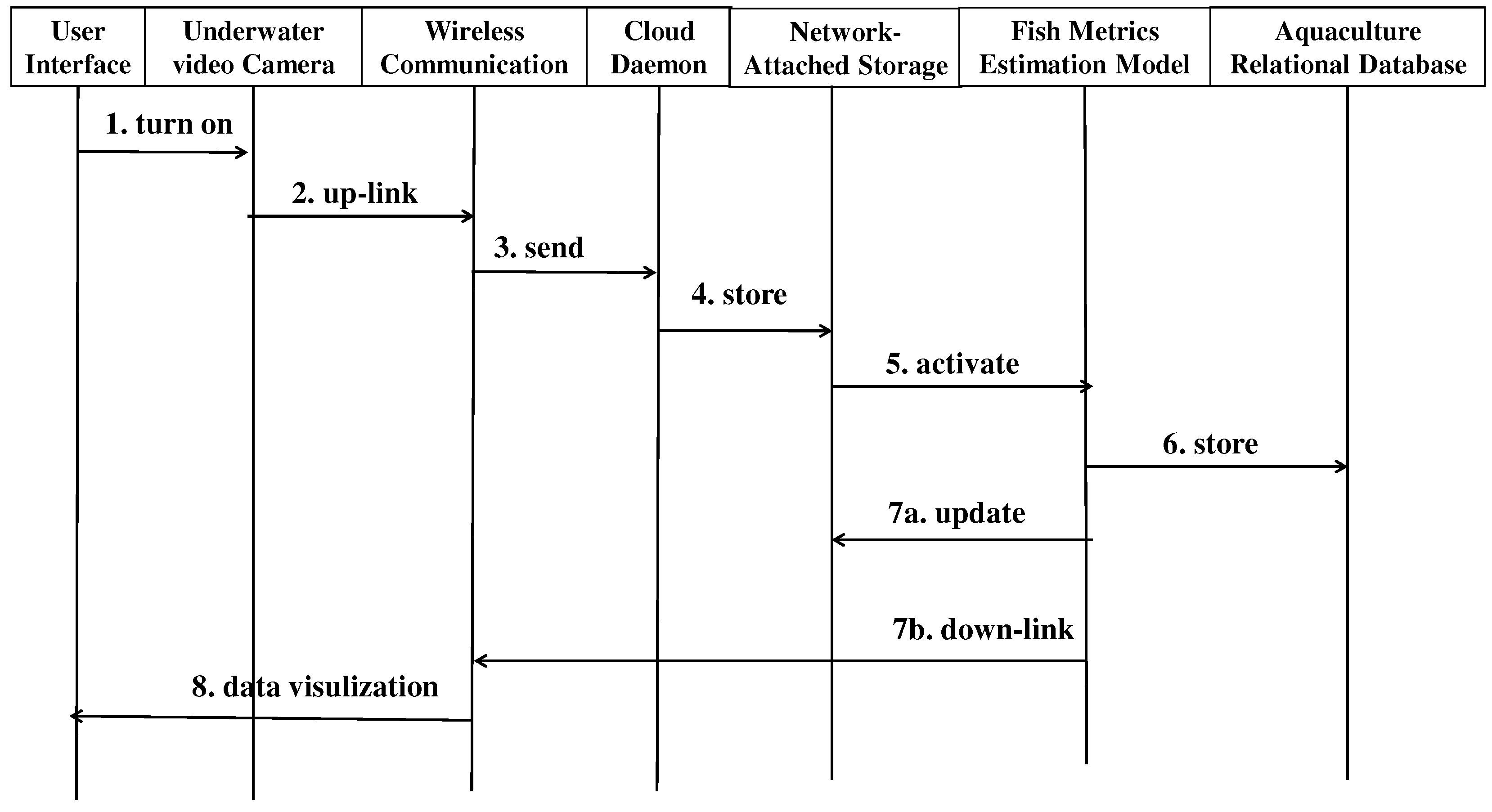
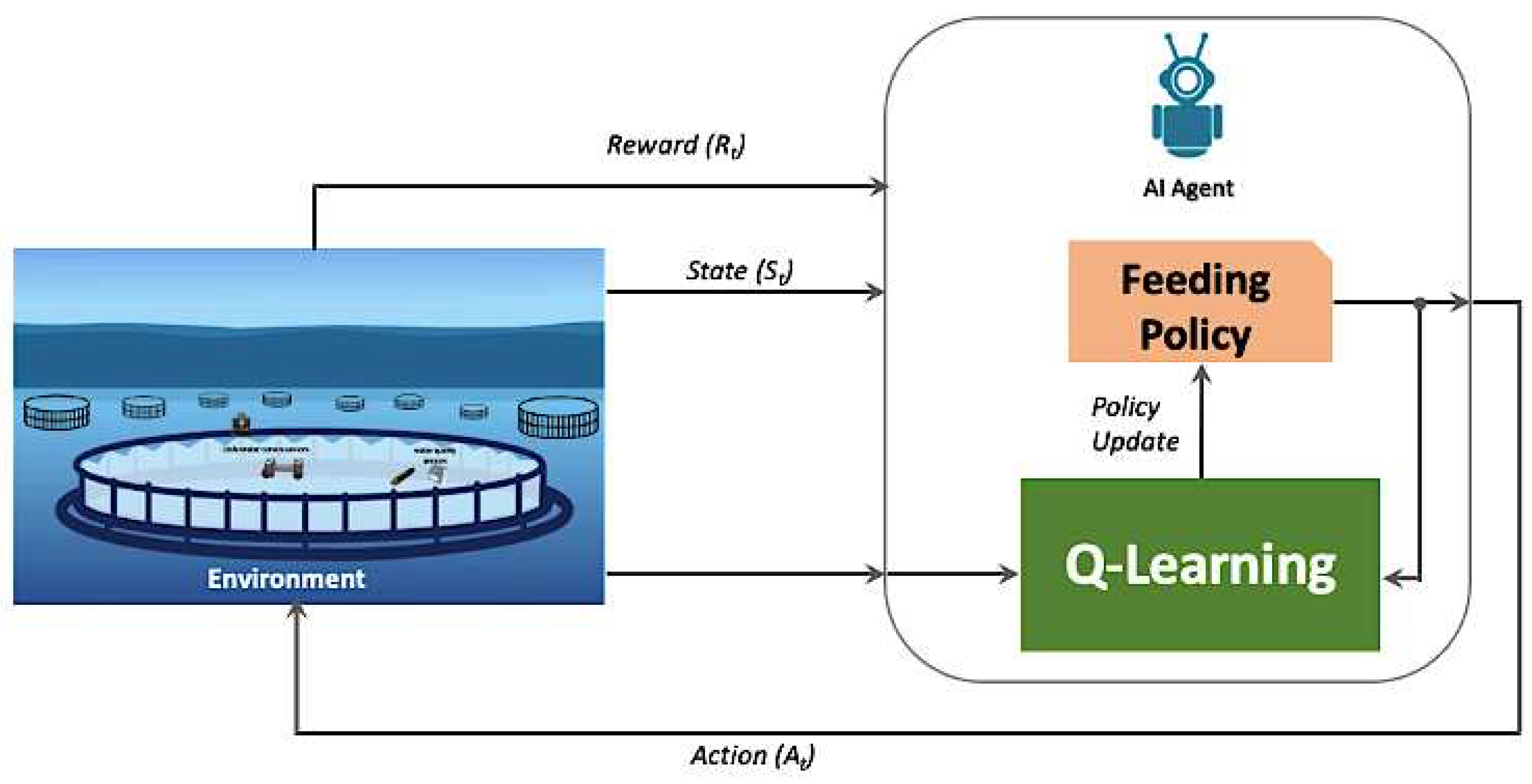
Algorithm 1: Q-Learning Policy Control Algorithm

Initialization: $Q\left(s,a\right), \forall s\in S, a\in \mathcal{A}\left(s\right),$arbitrarily, and $Q\left(terminal-state,.\right)=0$ Repeat (for each episode):   Initialize $S$   Repeat (for each step of the episode):     Choose $a$ from $\mathrm{s}$ using policy-derived $Q$ (e.g., $ϵ-$greedy)     Take action $a$, observe $r, s^{\prime }$     $Q\left(s,a\right)\leftarrow Q\left(s,a\right)+ \alpha \left[r+ \gamma ma{x}_{a}Q\left(s^{\prime },a\right)-Q\left(s,a\right)\right]$     $s \leftarrow s^{\prime }$; Until $s$ is terminal

The Q-value, denoted as Q(s, a), represents the weighted sum of future rewards associated with a particular state, s, and action, a. At each time step, the agent selects the action with the highest Q-value for the current state. Whenever an action is executed in the environment, the resulting new state and its corresponding reward are recorded in the Q-Table, along with information about the previous state and action. For decision-making, a random batch of stored experiences, consisting of state, action, reward, and next_state tuples, is retrieved and used for training. The Q-value, Q(s, a), is computed for the chosen action, and it is updated using Equation (6), where α represents the learning rate, controlling the extent of adaptation to new information. The variable r denotes the reward obtained from action a, while $ma{x}_{a}Q\left(s^{\prime }, \mathrm{a}\right)$ signifies the maximum predicted reward for the new state, $s^{\prime }$, considering all possible actions, $a^{\prime }$. The Q-learning framework is employed to seek the optimal policy that maximizes the expected reward value. The weights and biases of the agent's neural network are fine-tuned using gradient descent to align the network's output with the updated Q-values. Exploration of the optimal feeding policy is based on selecting the action with the highest reward value for a given state. This mechanism allows the agent to undergo training with a randomly sampled set of past experiences at each time step.

3. Results

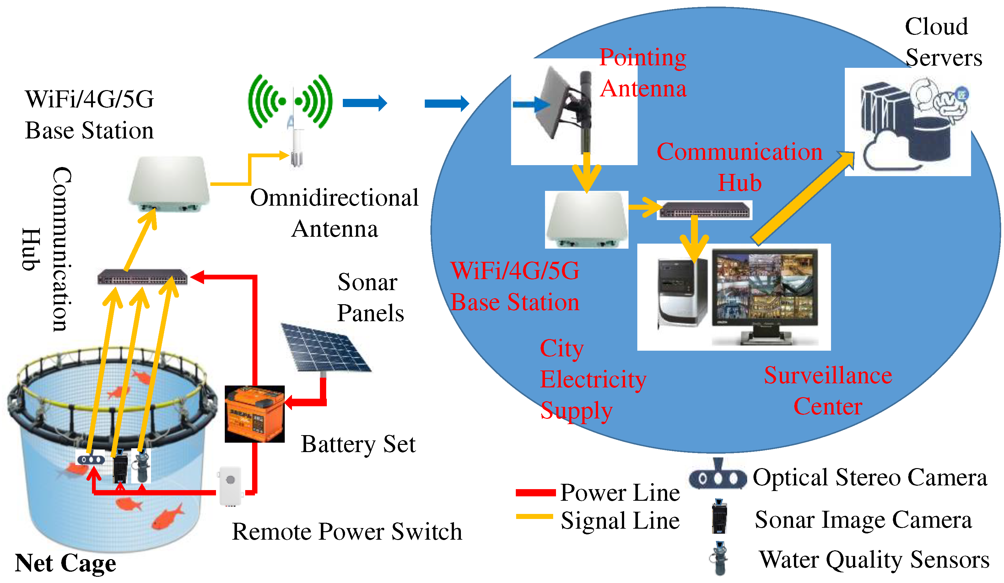
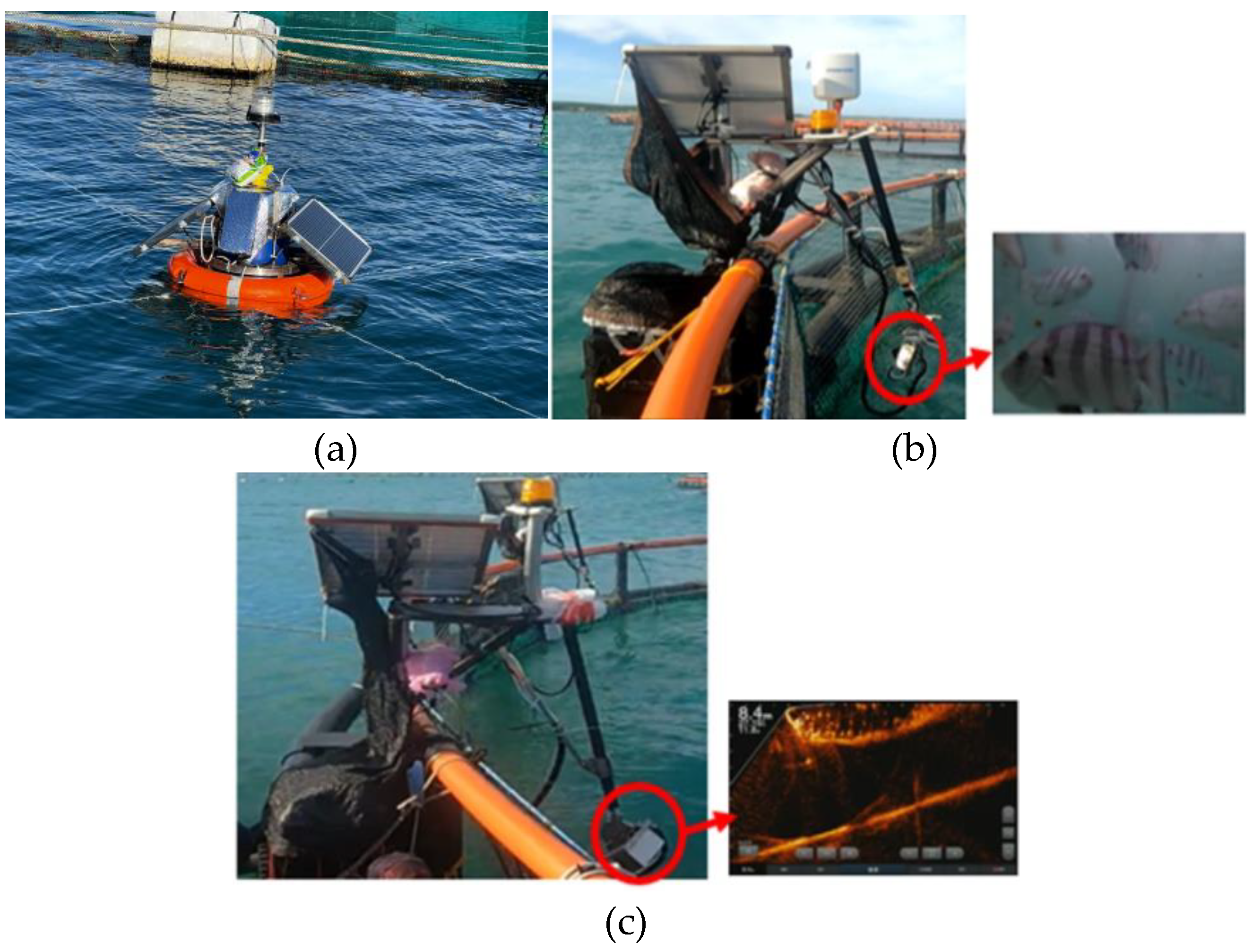
3.1. Experimental Devices and Set-up

Table 1. The pre-trained machine learning and deep learning models which provide AI functions in the DT objects of the proposed DT architecture for intelligent fish feeding management.

Table 1. The pre-trained machine learning and deep learning models which provide AI functions in the DT objects of the proposed DT architecture for intelligent fish feeding management.

DT Object	Machine Learning and Deep Learning Models	Physical/DT Objects
Water Quality Prediction	LSTM [37]	Salinity meter, dissolved oxygen meter, temperature sensing, water velocity meter, pH level meter
Fish Counting	YoLoV7 [38], MLP [36]	RGB Camera
Fish Length/Weight Estimation	Mask R-CNN[39], Optical Flow [40], KNN Regression [41],Principal Component Analysis (PCA) [42]	RGB Stereo Camera
Food Prediction	MLP [36]	Water Quality Prediction, Fish Counting, Fish Length/Weight Estimation
Fish Feeding Intensity Evaluation	Optical Flow [40], I3D Action Recognition [43]	RGB Stereo Camera
Fish Feeding Control	Q-Learning [32]	Automatic Feeding Machine, Fish Feeding Intensity Evaluation

This work used an RGB camera (Zed 2 2i stereo camera by Stereo Labs, France) to capture underwater images. GARMIN Panoptix Live Scope System (Garmin Ltd., Taiwan), with a sonar screen, a processor, and a sonar transducer probe, was utilized for the sonar camera system. In addition, we used the following water quality sensors: salinity meter, Y505-A dissolved oxygen meter, Y521 for temperature sensing, RS-232C water flow or velocity meter, and pH level for water quality data collection. All water quality sensors are under Yosemite Technologies except for the flow meter under Dalian Teren Instruments (DLTerren), and all were manufactured in China. These sensors capture environmental data and underwater surveillance videos from the experimental cages when the fish farmers operate the fish feeding process using a remote controllable feeding machine, deployed on a workboat.

As shown in Table 1, the digital architecture consists of nine DT objects integrated with different pre-trained machine learning and deep learning models for performing specific detection and prediction functions which optimize the fish feeding policy. However, we did not provide the completed details of the learning models since this study focuses on integrating digital twins with our cloud architecture and functionalities for intelligent fish feeding management. However, some details of the implementation can be found in our previous works, such as the fish feeding intensity evaluation [12], fish length and biomass estimation [14], fish count estimation [11], and water quality monitoring [13].

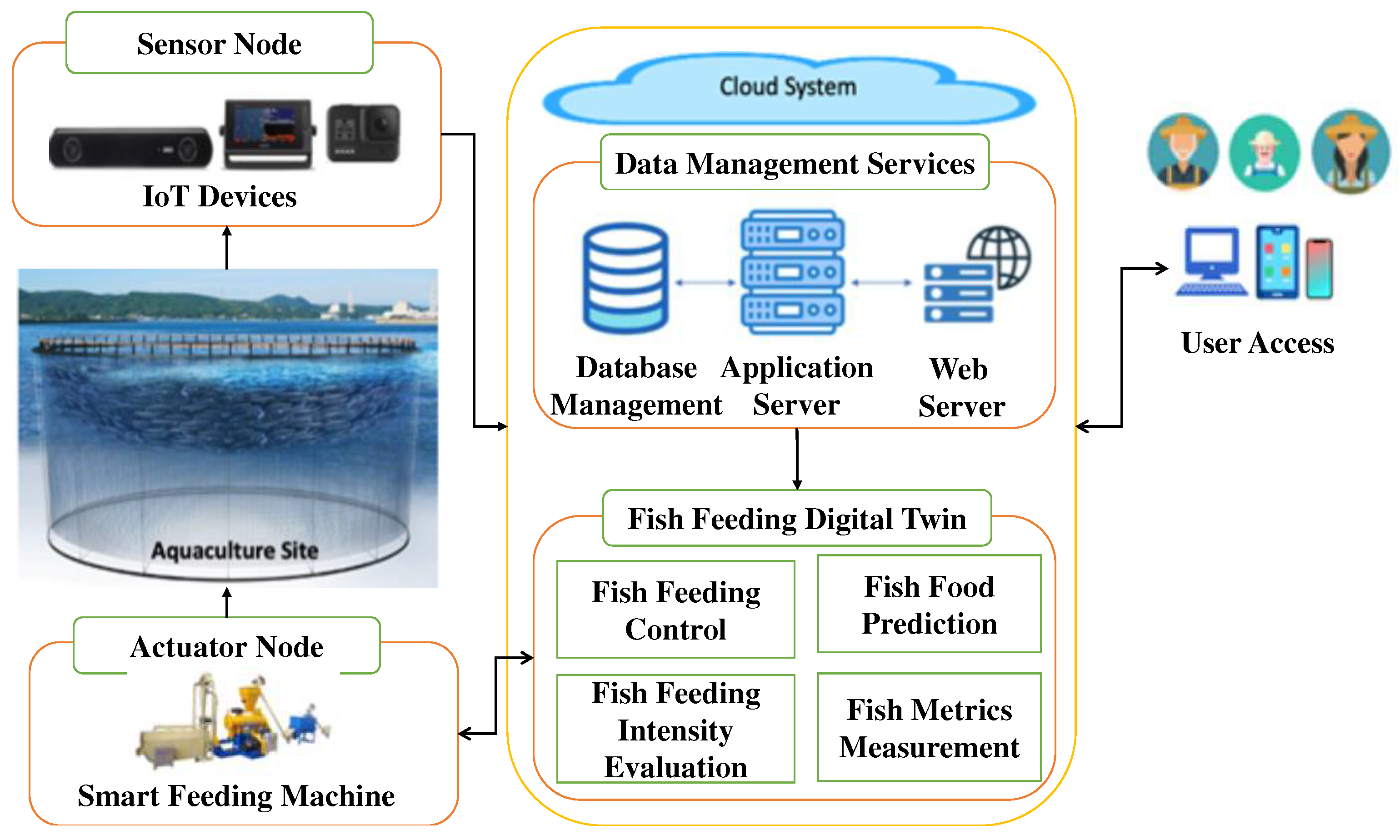
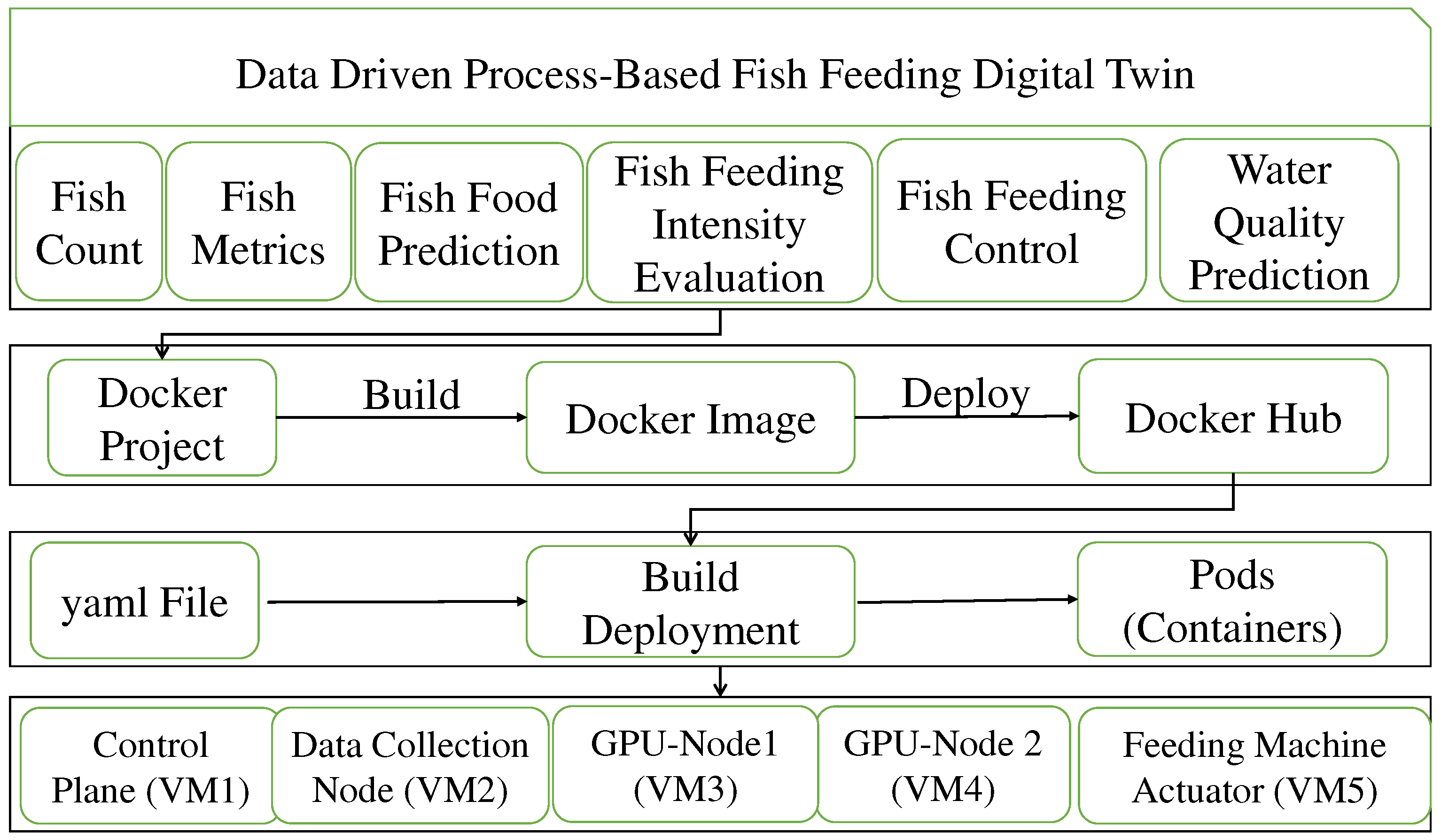
3.2. Implementation of the Cloud Computing Framework

Figure 11. Schematic diagram of the Kubernetes based cloud system architecture.

Figure 11. Schematic diagram of the Kubernetes based cloud system architecture.

The Digital Twin (DT) system relies on high-performance cloud computing infrastructure equipped with multiple GPU servers for parallel processing to achieve real-time decision-making. Our cloud system is implemented using Kubernetes (K8s) clusters for automated deployment, scaling, and management of containerized DT objects. Figure 11 illustrates the deployment architecture of the Digital Twin system in the cloud using Docker and Kubernetes (K8s). The current K8s environment consists of two hosts and three virtual machines, all running Linux Ubuntu servers. One of these virtual machines serves as the Master for Pod deployment, while the others function as worker nodes for running Pods. Docker, which functions as a lightweight virtual machine (VM), packages the program into image files. Once each component is converted into an image file, these images are pushed to a private repository and subsequently deployed in K8s by means of a configuration file. For each DT object, a dedicated code project is prepared, converted into an image file, and then deployed to K8s. The initial step involves creating a Dockerfile and building a Docker image for storage in the repository. In the K8s environment, a YAML file is authored to define the deployment, and the associated Docker image is linked to K8s for deployment across Pods or containers. The Docker container is integrated into the webpage, and it uses SSL certificates to securely connect to the database, ensuring the protection of webpage access. To establish the Kubernetes system, three computers were utilized, forming a robust infrastructure that can be accessed and controlled through the cloud. Table 2 outlines the hardware components used in the Kubernetes setup.

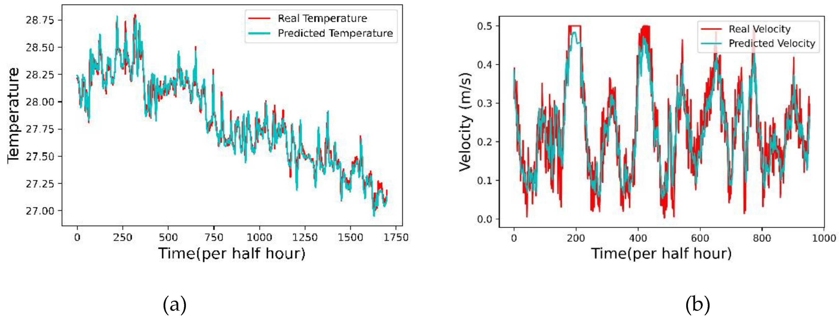
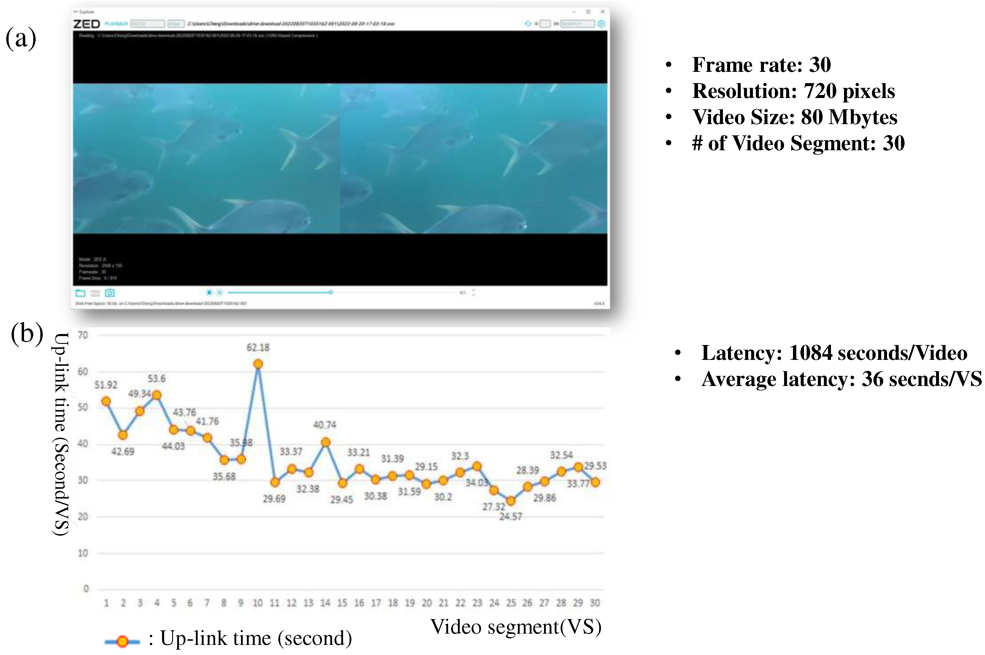
3.3. Experimental Results

Figure 12. Low cost sensor calibration using LSTM deep learning: (a) the result of water temperature; (b) the result of water velocity.

Figure 12. Low cost sensor calibration using LSTM deep learning: (a) the result of water temperature; (b) the result of water velocity.

To optimize the cost-effectiveness of the water quality monitoring system, this study introduces an AI buoy, as depicted in Figure 5(a), equipped with economical water quality sensors. These sensors autonomously transmit the collected data to the cloud-based water quality Digital Twin (DT) for further processing. The accuracy of data obtained from these low-cost sensors is calibrated using high-quality data acquired from precision instruments, albeit at a higher cost. Figure 12(a) and (b) illustrate the calibrated outcomes for water temperature and water velocity, achieved through Long Short-Term Memory (LSTM) deep learning models. This approach results in a cost-effective design for the proposed water quality monitoring DT. The system has undergone deployment and validation in our experimental net cage farms for a minimum duration of six months.

Figure 13 displays an example stereo video capture, which is automatically transmitted to the cloud via a 4G telecommunication network for fish counting, fish length and weight estimation, and fish feeding intensity evaluation. The underwater video is recorded during the fish feeding process, typically lasting about half an hour for a large net cage. To facilitate efficient data transmission, an end-computing system is equipped with our stereo camera. It employs the MPEG-4 video coding scheme to compress the captured video, reducing its size to approximately 80 megabytes, which is subsequently segmented into 30 segments. This results in a bandwidth requirement of approximately (80×8)⁄30, which is approximately equal to the average up-link data rate of a commercial 4G network, approximately 24.92 Mbps. Ideally, our system is designed to transmit each video segment in real-time, with the target latency for transmitting a stereo video comprising 30 segments being 30 seconds. However, as depicted in Figure 12(b), the average up-link data rate of the commercial 4G network falls significantly below 24.92 Mbps in real-world environments. To address this challenge, we recommend incorporating a 5G network router into our end-computing module for underwater video surveillance in the future. In this scenario, the cloud daemon can receive the surveillance video in real-time, as the up-link rate of a 5G network is approximately ten times that of a 4G network.

Figure 13. The results of the underwater video data collection DT which captures a stereo video from the experimental cage, which is then sent to the cloud through the public 4G telecommunication network.

Figure 13. The results of the underwater video data collection DT which captures a stereo video from the experimental cage, which is then sent to the cloud through the public 4G telecommunication network.

Table 3. The food eaten ratio of the fish feeding intensity levels.

Table 3. The food eaten ratio of the fish feeding intensity levels.

Strong	Medium	Weak	Normal
1.0	0.7	0.6	0.2

Upon receiving an underwater video, the daemon initiates the Fish Counting DT, Fish Metrics DT, and Fish Feeding Intensity Evaluation DT modules. These modules are responsible for generating the fish count, fish length and weight measurements, and assessing the feeding intensity level. The error rates associated with these DT objects, which are implemented using deep learning models presented in our previous research works [11,12,14], are described as follows.

• The Fish Counting DT exhibits a 4% error rate. This DT module utilizes optical underwater video as input, employing the YOLOv7 deep learning object detector to identify fish objects within individual frames. Subsequently, it feeds the time-series fish counts into an MLP regression model for fish count prediction. To ensure the accuracy of prediction results, it is essential to accurately record the initial fish count and the number of deceased fish. In the event that the ground truth for fish count changes, the MLP regression model undergoes re-training accordingly.
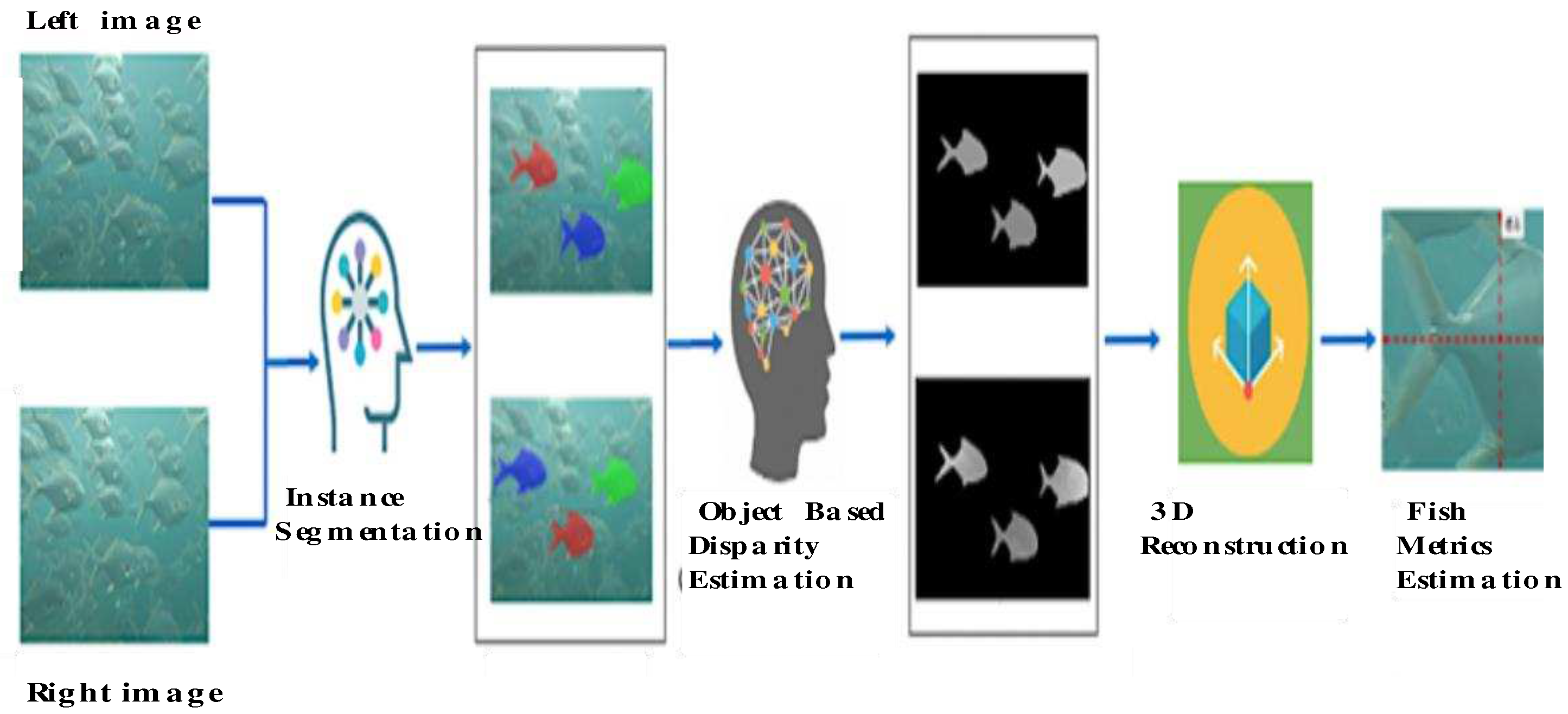
• The Fish Metrics DT modules estimate fish length and height using the input stereo video. This process involves acquiring implicit and explicit camera parameters through a camera calibration algorithm [44], followed by the segmentation of fish objects in the rectified left and right frames using MaskRCNN [39]. The segmented objects in the left image are then matched with corresponding objects in the right image, and an optical flow deep learning model [40] is employed to establish pixel correspondences for each matched object pair. Pixel-wise disparity and dense values are computed based on the calibrated camera parameters, facilitating 3D fish object reconstruction. Finally, Principal Component Analysis (PCA) [42] is applied to estimate fish length and height. Additionally, this study includes a human-labeled dataset, with each record containing information on fish length, height, and weight. Leveraging the estimated fish length and height alongside this dataset as inputs, we utilize the K-NN regression model [41] to predict fish weight. Notably, the error rate associated with fish weight estimation is approximately 12%.
• The Fish Food DT employs an MLP regression model, as depicted in Figure 8, to forecast the daily food requirements for executing the fish feeding process. To align the actual daily food consumption observed in real-world fish feeding operations with the outputs of the aforementioned DT objects, a dedicated training dataset is meticulously curated for training the food prediction model. Empirical findings indicate that the food prediction model exhibits an error rate of approximately 2%.
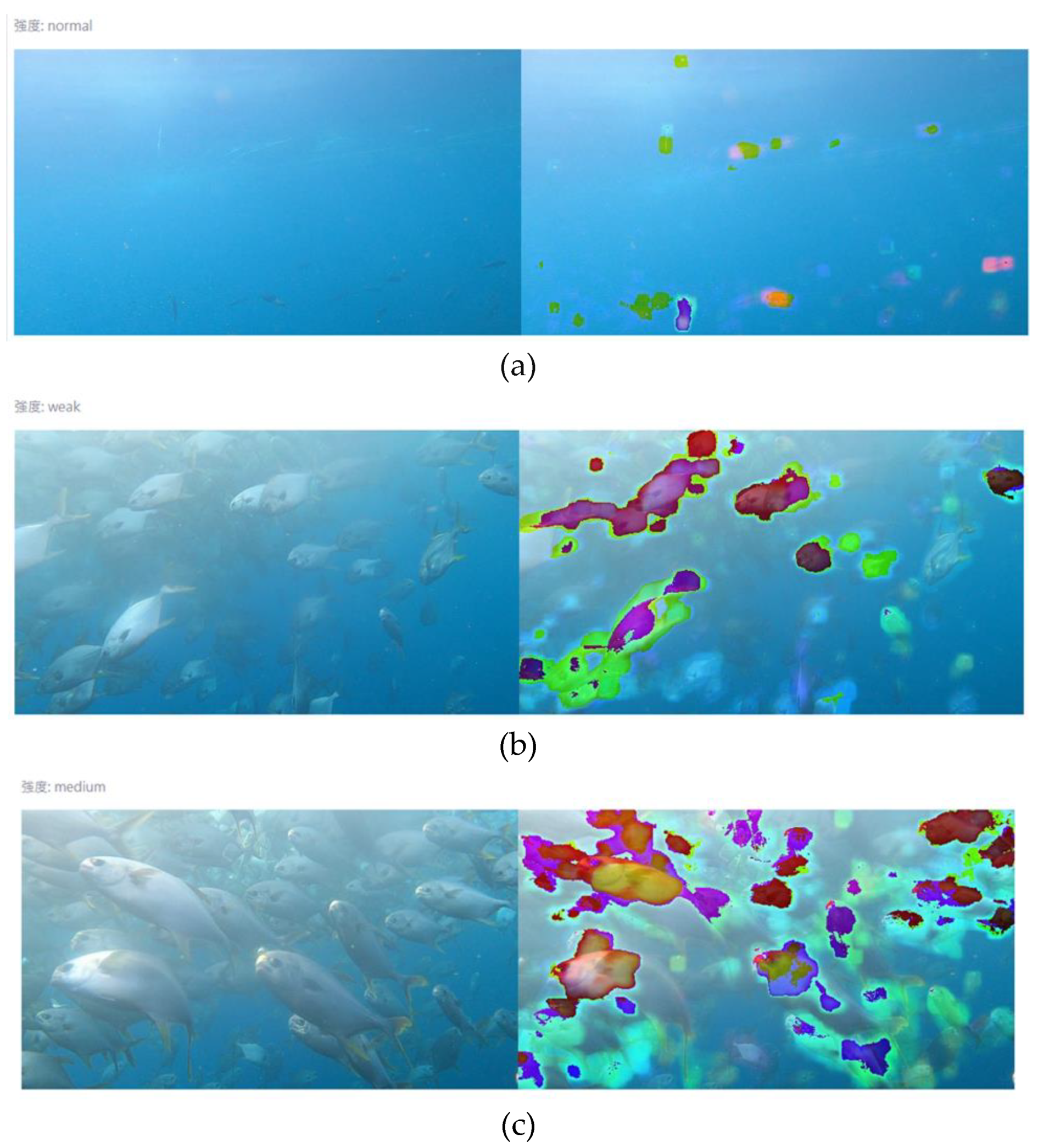
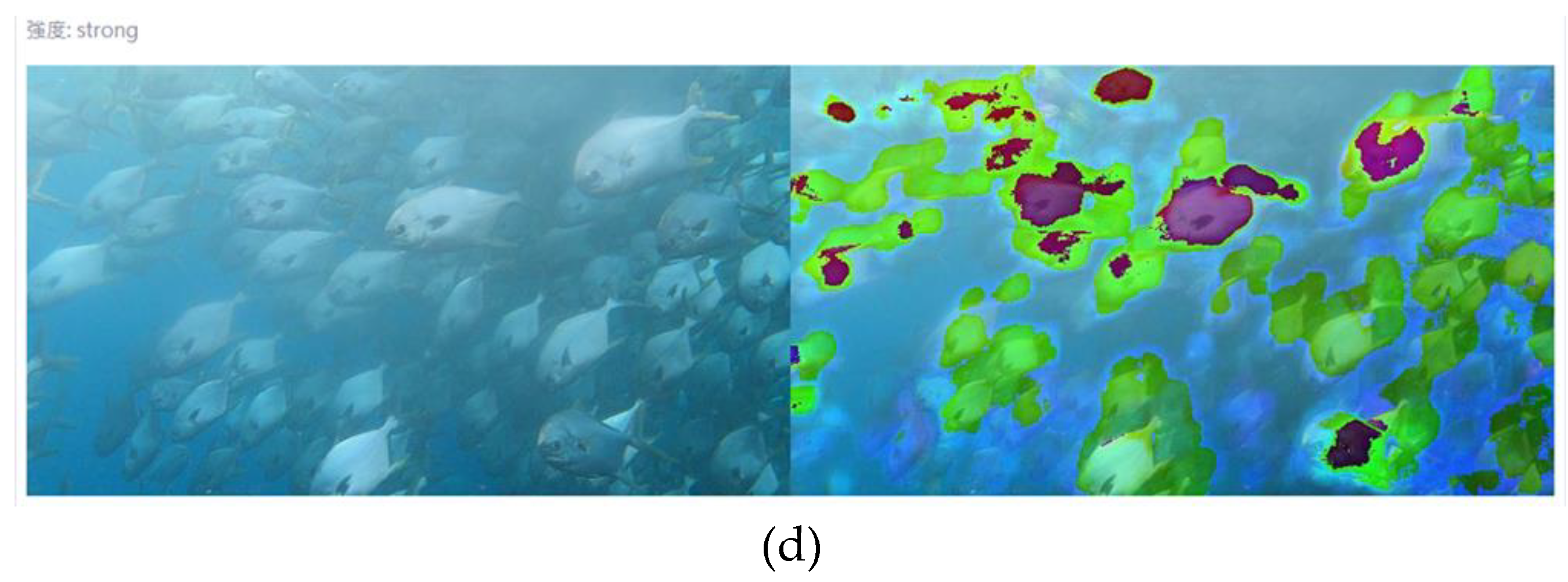
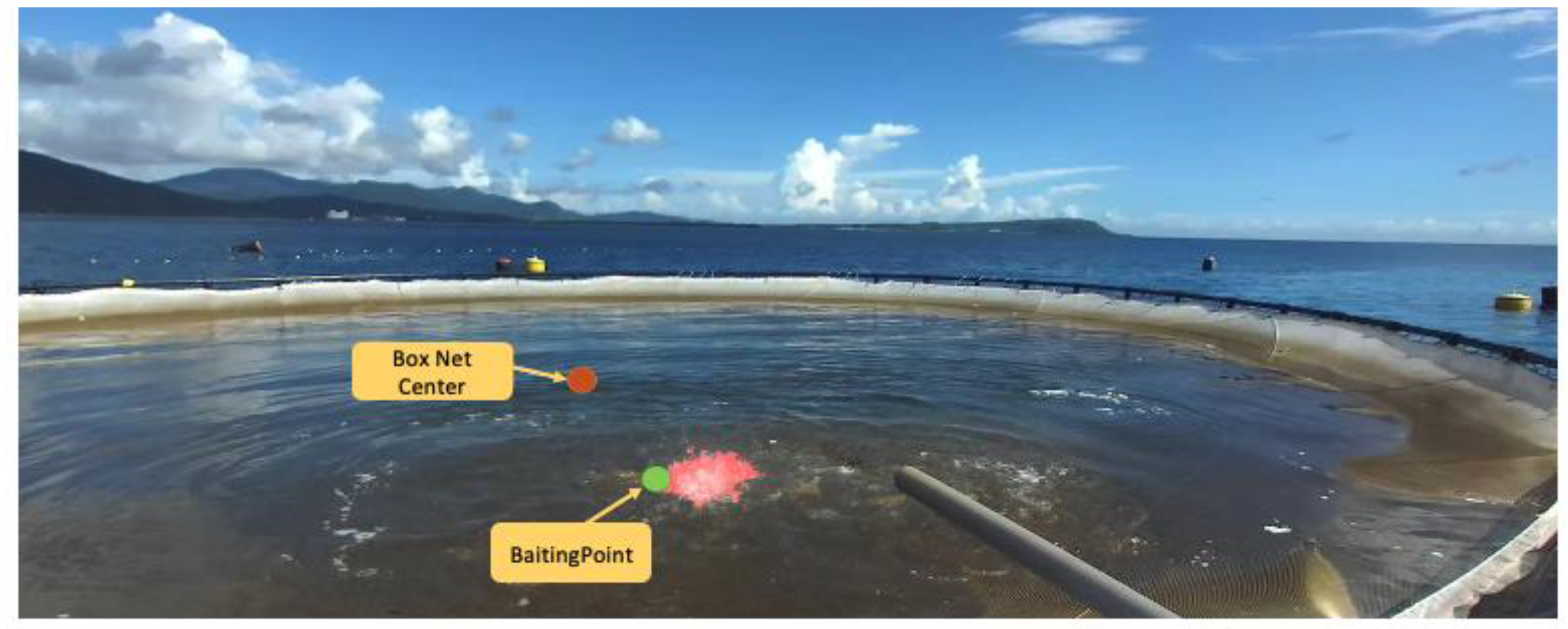
• The DT object for fish feeding intensity evaluation is designed to minimize residual food through the fish feeding control algorithm. In practice, the daily fish food for feeding is initially separated into 5 to 10 parts. The fish feeding control algorithm then uses our smart feeding machine to send food into the cage part-by-part. For each part feeding, the state of fish feeding intensity is evaluated to determine the scaling factor of fish food for the next part feeding by looking up Table 3. The results are also monitored across frames in Figure 14, showing how the fish movement intensity varies from frame to frame. When feed is fed to the fish, they initially move faster to grab food at the water's surface. Eventually, their movement decreases or stops as their appetite gradually declines when they are almost sated. Thus, the speed of fish movement is used to define their feeding level. In this work, we classified fish feeding intensity into four levels: weak, normal, medium, and strong, as presented in Figure 15. The left image shows the exact image captured from the aquaculture farm, and the right image is the result of the analysis of the fish motions. The second image with fewer color masks shows a normal fish movement or no feeding being performed. Details on how fish feeding intensity is modeled and implemented are fully described in our other works on fish feeding intensity evaluation [12]. The error rate of the fish feeding evaluation model is about 95.8% based on the human-labeled training dataset.

Figure 14. Real-time fish feeding intensity evaluation based on optical flow of underwater surveillance video: (a) ‘Normal’; (b)’ ‘Weak’; (c) ‘Medium’; (d) ‘Strong’.

Figure 14. Real-time fish feeding intensity evaluation based on optical flow of underwater surveillance video: (a) ‘Normal’; (b)’ ‘Weak’; (c) ‘Medium’; (d) ‘Strong’.

Our smart feeding machine is equipped with a programmable gun barrel designed for precision fish feeding. Figure 15 illustrates how the gun barrel is dynamically positioned throughout the feeding process, leveraging splash detection from surface water surveillance video. This innovative feed delivery mechanism ensures minimal food wastage, as it is precisely aimed at the fish's location. Furthermore, our system employs sonar technology to detect fish positions in the underwater environment, complemented by a stereo camera system capturing images of the cage water surface, as depicted in Figure 16. This setup provides access to the fish-feeding user interface. The prediction results of fish feeding intensity can also serve as a valuable metric for evaluating fish vitality. Fish schools exhibiting fast swimming speeds are indicative of robust vitality levels. The analysis of fish vitality offers insights into their feeding appetites and eating behavior during the feeding period. Farmers can use this information to make informed decisions about continuing feeding with the smart fish-feeding machine. Additionally, it provides data on feeding duration, vitality levels, and suggestions for optimizing feeding procedures. In parallel, our system maintains a feeding inventory that tracks cumulative feeding amounts and remaining food supplies. This feature aids farmers in assessing feed sufficiency and determining when to replenish their stocks. Moreover, the feeding record feature compiles data on the average fish weight, fish count in the cage during feeding, the type of feed used, and estimated feeding quantities based on both fish feeding predictions and actual amounts dispensed. It also includes the duration of the feeding session. These feeding records are instrumental in storing historical feeding data, which can be uploaded to the platform's cloud storage. This dataset serves as a valuable resource for training machine learning and deep learning prediction models, ultimately contributing to the development of expert systems in aquaculture management.

Figure 15. Fish location analysis for the best position in dispensing feeds using the smart feeding machine gun barrel.

Figure 15. Fish location analysis for the best position in dispensing feeds using the smart feeding machine gun barrel.

Figure 16. The user interface for intelligent fish feeding management: (a) fish vitality analysis; (b) feed inventory; (c) feeding record.

Figure 16. The user interface for intelligent fish feeding management: (a) fish vitality analysis; (b) feed inventory; (c) feeding record.

4. Discussion

5. Conclusions

References

1. Li, H.; Chatzifotis, S.; Lian, G.; Duan, Y.; Li, D.; Chen, T. Mechanistic Model based Optimization of Feeding Practices in Aquaculture. Aquacultural Engineering 2022, 97, 102245. [CrossRef]
2. Flinn, S. A; Midway, S. R. Trends in Growth Modeling in Fisheries Science. Fishes 2021 , 6(1), 1. [CrossRef]
3. DeVries, D.A.; Grimes, C.B. Spatial and Temporal Variation in Age and Growth of King Mackerel, Scomberomorus Cavalla, 1977–1992. Fish. B-NOAA 1997, 95, pp. 694–708. [CrossRef]
4. Helser, T.E.; Lai, H.L. A Bayesian Hierarchical Meta-analysis of Fish growth: With an Example for North American largemouth Bass, Micropterus salmoides. Ecol. Model. 2004, 178, pp. 399–416. [CrossRef]
5. Midway, S.R.; Wagner, T.; Arnott, S.A.; Biondo, P.; Martinez-Andrade, F.; Wadsworth, T.F. Spatial and Temporal Variability in Growth of Southern Flounder (Paralichthys lethostigma). Fish. Res. 2015, 167, pp. 323–332. [CrossRef]
6. Ubina, N. A.; Lan H.-Y. ; Cheng, S.-C.; Chang C.-C.; Lin, S.-S.; Zhang K.-X.; Lu, H.-Y.; Cheng, C.-Y.; Hsieh, Y.-Z. Digital Twin-based Intelligent Fish Farming with Artificial Intelligence Internet of Things (AIoT). Smart Agricultural Technology 2023, 5, 100285. [CrossRef]
7. Ubina, N.; Cheng, S.-C. A review of unmanned system technologies with its application to aquaculture farm monitoring and management. Drones 2022, 6(1), 12. [CrossRef]
8. Manoharan, H.; Teekaraman, Y.; Kshirsagar, P. R.; Sundaramurthy, S.; Manoharan, A. Examining the Effect of Aquaculture Using Sensor-based Technology with Machine Learning Algorithm. Aquaculture Research 2020, 51(11), 4748–4758. [CrossRef]
9. Yang, X. T.; Zhang, S.; Liu, J. T.; Gao, Q. F.; Dong, S. L.; Zhou, C. Deep Learning for Smart Fish Farming: Applications, Opportunities and Challenges. Rev Aquaculture 2021, 13 (1), pp. 66-90. [CrossRef]
10. Naomi A.; Cheng, S.-C. Chen, H.-Y.; Chang, C.-C.; Lan, H.-Y. A Visual Aquaculture System Using a Cloud-based Autonomous Drones. Drones 2021, 5(4), 109. [CrossRef]
11. Chang, C.-C.; Wang, Y.-P.; Cheng, S. C. (2021, Nov). Fish Segmentation in Sonar Images by Mask R-CNN on Feature Maps of Conditional Random Fields. Sensors 2021, 21(22), 7625. [CrossRef] [PubMed]
12. Ubina, N.; Cheng, S.-C.; Chang, C.-C.; Chen, H.-Y. Evaluating Fish Feeding Intensity in Aquaculture with Convolutional Neural Networks. Aquac. Eng. 2021, 94, 102178. [CrossRef]
13. Lu, H.-Y.; Cheng, C.-Y; Cheng, S.-C.; Cheng, Y.-H.; Lo, W.-C.; Jiang, W.-L.; Nan, F.-H.; Chang, S.-H.; Ubina, N. A. Low-cost AI Buoy System for Monitoring Water Quality at Offshore Aquaculture Cages. Sensors 2022, 22(11), 4078. [CrossRef] [PubMed]
14. Ubina, A.; Cheng, S.-C.; Chang, C.-C.; Cai, S.-Y.; Lan, H.-Y.; Lu, H.-Y. Intelligent Underwater Stereo Camera Design for Fish Metric Estimation Using Reliable Object Matching. IEEE Access 2022, 10, pp. 74605-74619. [CrossRef]
15. Li, D.; Wang, Q.; Li, X.; Niu, M.; Wang, H.; Liu, C. Recent Advances of Machine Vision Technology in Fish Classification. ICES J. Mar. Sci. 2022, 79, pp. 263–284. [CrossRef]
16. Kuswantori, A.; Suesut, T.; Tangsrirat, W.; Schleining, G.; Nunak, N. Fish Detection and Classification for Automatic Sorting System with an Optimized YOLO Algorithm. Appl. Sci. 2023, 13, 3812. [CrossRef]
17. Ferko, E.; Bucaioni, A.; Beham, M. Architecting Digital Twins. IEEE Access 2022, 10, pp. 50335-50350. [CrossRef]
18. Jacoby, M.; Usländer, T. Digital twin and Internet of Things—Current standards landscape. Applied Sciences 2020, Volume 10(18), 6519. [CrossRef]
19. Minerva, R.; Lee, G. M.; Crespi, N. Digital Twin in the IoT Context: A Survey on Technical Features, Scenarios, and Architectural Models. Proceedings of the IEEE 2020, 108(10), pp. 1785-1824. [CrossRef]
20. Nasirahmadi, A.; Hensel, O. Toward the Next Generation of Digitalization in Agriculture Based on Digital Twin Paradigm. Sensors 2022, 22(2), 498. [CrossRef]
21. Chang, C.-C.; Ubina, N.A.; Cheng, S.-C.; Lan, H.-Y.; Chen, K.-C.; Huang, C.-C. A Two-Mode Underwater Smart Sensor Object for Precision Aquaculture Based on AIoT Technology. Sensors 2022, 22(19), 7603. [CrossRef]
22. Wang, C.; Li, Z.; Wang, T.; Xu, X.; Zhang, X.; Li, D. Intelligent fish farm—the future of aquaculture. Aquaculture International 2021, Volume 29, pp. 2681-2711. [CrossRef] [PubMed]
23. Lima, A.; Royer, E.; Bolzonella, M.; Pastres, R. Digital Twins for Land-based Aquaculture: A Case Study for Rainbow Trout (Oncorhynchus mykiss). Open Research Europe 2023, 28(2), 16. [CrossRef]
24. Lan, H.-Y.; Afero, F.; Huang, C.-T.; Chen, B.-Y.; Huang, P.-L.; Hou, Y.-L. Investment Feasibility Analysis of Large Submersible Cage Culture in Taiwan: A Case Study of Snubnose Pompano (Trachinotus anak) and Cobia (Rachycentron canadum). Fishes 2022, 7, 151. [CrossRef]
25. Somers, I. F. On a Seasonally Oscillating Growth function. Fishbyte 1998, 6 (1), pp. 8-11.
26. Gompertz, B. On the Nature of the Function Expressive of the Law of Human Mortality, and on a New Mode of Determining the Value of Life Contingencies. Philosophical Transactions of the Royal Society of London 1825, 115, pp. 513-583. [CrossRef]
27. Lipkin, L.; Smith, D. Logistic Growth Model - Background: Logistic Modeling. Mathematical Association of America. https://www.maa.org/press/periodicals/loci/joma/logistic-growth-model-background-logistic-modeling (accessed March 22, 2023).
28. Quinn, T. J.; Deriso, R. B. Quantitative Fish Dynamics (Biological Resource Management). Oxford University Press, 1999.
29. Pauly, D. The Relationships between Gill Surface Area and Growth Performance in Fish: a Generalization of von Bertalanffy's Theory of Growth. Meeresforsch 1981, 28, pp. 251-282.
30. Ursin, E. A Mathematical Model of Some Aspects of Fish Growth, Respiration, and Mortality. Journal of the Fisheries Research Board of Canada 1967, 24, pp. 2355-245. [CrossRef]
31. Yang, Y. A Bioenergetics Growth Model for Nile Tilapia (Oreochromis Niloticus) Based on Limiting Nutrients and Fish Standing Crop in Fertilized Ponds. Aquacult Eng. 1998, 18 (3), pp. 157-173. [CrossRef]
32. Chahid, A.; N'Doye, I.; Majoris, J. E.; Berumen, Michael L.; Laleg-Kirati, T.-M. Fish Growth Trajectory Tracking Using Q-learning in Precision Aquaculture, Aquaculture 2022, 550, 737838. [CrossRef]
33. Liu, C.; Ding, J.; Sun, J. Reinforcement Learning Based Decision Making of Operational Indices in Process Industry Under Changing Environment. IEEE Transactions on Industrial Informatics 2021, 17 (4), pp. 2727-2736. [CrossRef]
34. Jananpa, P. C.; Takada, R.; de Freitas, T. M.; Pereira, M.M.B.; Sá-Freire, L.; Lugert, V.; Sartuuri, C.; Pereira, M. M. Nonlinear Regression Analysis of Length Growth in Cultured Rainbow Trout. Arquivo Brasileiro de Medicina Veterinária e Zootecnia 72(5):1778-1788. [CrossRef]
35. Zhou, H. et al. Informer: Beyond Efficient Transformer for Long Sequence Time-Series Forecasting. The Thirty-Fifth AAAI Conference on Artificial Intelligence (AAAI-21), February 2-9, 2021, 2021. [CrossRef]
36. Qin, Y; Li. C,; Shi, X; Wang, W. MLP-Based Regression Prediction Model For Compound Bioactivity. Front Bioeng Biotechnol. 2022, 10, 946329. [CrossRef]
37. Hochreiter, S.; Schmidhuber, J. Long Short-term Memory. Neural computation 1997, 9, pp. 1735-1780. [CrossRef]
38. Wang, C.-Y.; Bochkovskiy, A.; Liao, M. H.-Y. YOLOv7: Trainable Bag-of-freebies Sets New State-of-the-art for Real-time Object Detectors. Proc. IEEE/CVF Conference on Computer Vision and Pattern Recognition (CVPR) 2023. [CrossRef]
39. He, K.; Gkioxari, G.; Dollár, P.; Girshick, R. Mask R-CNN. Proc. IEEE International Conference on Computer Vision 2017.
40. Teed, Z.; Deng, J. RAFT: Recurrent All-Pairs Field Transforms for Optical Flow. Proc. Of the Thirtieth International Joint Conference on Artificial Intelligence 2021. [CrossRef]
41. Campos, G. O.; Zimek, A.; Sander, J.; Campello, R. J. G. B.; Micenková, B.; Schubert, E.; Assent, I.; Houle, M. E. On the Evaluation of Unsupervised Outlier Detection: Measures, Datasets, and an Empirical Study. Data Mining and Knowledge Discovery 2016, 30 (4), pp. 891–927. [CrossRef]
42. Jolliffe, I. T. Principal Component Analysis, Springer-Verlag New York, 2002.
43. Carreira, J.; Zisserman, A. Quo Vadis, Action Recognition? A New Model and the Kinetics Dataset. Proc 2017 IEEE/CVF Conference on Computer Vision and Pattern Recognition (CVPR) 2017.
44. Ding, W.; Liu, X.; Xu, D.; Zhang, D.; Zhang. Z. A Robust Detection Method of Control Points for Calibration and Measurement with Defocused Images. IEEE Transactions on Instrumentation and Measurement 2017, 66(10), pp. 2725–2735. [CrossRef]
45. Lall, S. P.; Tibbetts, S. M. Nutrition, Feeding, and Behavior of Fish, Veterinary Clinics of North America. Exotic Animal Practice 2009, 12 (2), pp. 361-372. [CrossRef]