Improve the quality of Industrial Robot Control Using an Iterative Learning Method with Online Optimal Learning and Intelligent Online Learning Function Parameters

It is unavoidable that the characteristics of the robot system alter inexactly or cannot be correctly determined during movement and are impacted by external disturbances. There are many adaptive control methods, such as sliding control or neural control, to improve the quality of trajectory tracking for robot motion systems. Still, those methods require a large amount of computation related to solving the problem of constrained nonlinear optimization problem. The article presents some techniques for determining an intelligent controller's online learning function parameters, including two circuits: the inner circuit is a state feedback linearized controller, and the outer course is an Interactive learning controller and does not use the robot's mathematical mode with function parameters online optimal learning and intelligent online learning closely following the joint model to stabilize the robot system. Finally, the 2-DOF planar robot simulation is performed on Matlab software R2022b. The findings indicate that outstanding tracking performance is achievable.

Keywords:

Subject: Engineering - Other

1. Introduction

Robots have been widely used in many industrial fields, so countless robot control methods have been researched and applied, helping robots achieve accurate trajectory tracking. However, these methods are all built based on the mathematical model describing the robot, and they are classified depending on the level of accuracy of that mathematical model. The Euler - Lagrange model is a form of mathematical model often used for developing and synthesizing controllers, and it is impacted by external input noise d(t) as follows:

\underline{u} + \underline{d} = M (\underline{q}, \underline{θ}) \ddot{\underline{q}} + C (\underline{q}, \dot{\underline{q}}, \underline{θ}) \dot{\underline{q}} + G (\underline{q}, \underline{θ}) + F (\underline{\dot{q}}, \underline{θ})

(1)

In which

\underline{q}

is the vector of joint variables;

\underline{θ}

is the vector of uncertain parameters;

M (\underline{q}, \underline{θ})

is the inertia matrix that is always positive definite symmetry;

C (\underline{q}, \dot{\underline{q}}, \underline{θ})

is the vector of Coriolis and centrifugal components;

F (\underline{\dot{q}}, \underline{θ})

describes the effect of friction;

G (\underline{q}, \underline{θ})

is the vector gravity;

\underline{d} (t)

is the noise vector in the actuator and you is the control signal.

With the matching variables equal to the number of input signals, such a robot system has enough actuators. The robot control task is to build a feedback controller so that the output is the joint variables

\underline{q}

that follow the desired trajectory

\underline{r} (t)

and the tracking quality does not depend on uncertain parameters and components and external noise

\underline{d} (t)

. Over time, due to many objective factors, such as equipment wear and tear from environmental impacts, the initially set design quality is no longer guaranteed. In this case, it is common to rebuild the controller. As we know, to design an industrial robot motion control system using the traditional method, one thing that cannot be changed is to always clearly understand the control object, which means the control object must be controlled and expressed in modeling in the form of some mathematical model that accurately describes the object, which here can be a transfer function and can also be a state model in the form of a system of differential equations-highest classification. At the same time, when building and designing a motion control system, it is necessary to anticipate objective factors that will not impact the system as expected, such as external interference, etc., leading to damage to the system. The control is no longer as effective as before, and one must redefine the mathematical model of the control object, re-evaluate the rules of unwanted effects, bring objectivity into the system, Rebuild the controller, or at least redefine the parameters for the controller. There have been many control methods to solve the above problem, for example, the exact linearization method [1]. If the external noise component

\underline{q}

passes, but the indeterminate constant parameter still exists, we have the inverse control method of the model [2]. In cases where both external noise components and uncertain constant parameters exist, there is a sliding control method [3]. However, the disadvantage of the sliding control method is the phenomenon of chattering when the system slides on the sliding surface at a high frequency. To improve this vibration phenomenon, there is also a high-order sliding control method [4], but it still requires an estimated value of the maximum standard deviation of the model caused by and

\underline{d} (t)

and cannot eliminate it. Due to vibration, there is still a risk of premature failure of robot mechanical equipment components. To overcome the above disadvantages, intelligent control methods can be used, such as the control trend of not using the robot's dynamic model (1), so the control quality is not affected. by components

\underline{q} (t)

) and

\underline{d} (t)

.The intelligent control method mainly applied to robots mentioned in the article is the iterative learning method [5]. This integrated control method with cyclic working systems requires the same state. At the same time, the parameters

\underline{q} (t)

) and

\underline{d} (t)

are also required to be periodic and have the exact change period as the working cycle of industrial robots. The primary iterative learning control method is only sometimes applied to meet the desired control quality. There have been many improvements to iterative learning to improve control quality and expand the scope of practical applications. The first improvement is the improvement of combining iterative learning with traditional control methods, often called indirect iterative learning or direct transmission iterative learning. These improvements include [6] when the friction component alone cannot be determined, [7] when that is not possible, or [8] when the learning function parameters cannot be found, as well as when the learning function parameters need to be changed. Change during work cycles. A control trend for a class of robotic systems is model matching control, including [9]. This control method requires the mathematical model (1), which will encounter problems and disadvantages of previous traditional control methods. The next improvement is to use model-based control but almost entirely not use the mathematical model (1) of the robot, applicable to both cases where

\underline{q} (t)

) and

\underline{d} (t)

are dependent. It depends on time and does not require periodicity, so it can be considered an intelligent model-matching control method. This method is based on theoretical results on optimal control of each segment on the time axis available in [10] and applying disturbance estimation to control self-balancing two-wheeled vehicles [11].

The main content of the article is to analyze and evaluate additional improvements to essential iterative learning to improve the quality of motion control of robot systems and expand the scope of practical applications, specifically, Intelligent control based on model matching (model matching) almost wholly does not need to use the mathematical model of the robot system, applicable to the case where

\underline{q} (t)

) and

\underline{d} (t)

depends on time, no need for circulation for the robot system. The content of the article includes six parts. Part 1 is the problem of researching iterative learning for robot systems. Part 2 presents the results of the 2-DOF robot dynamic equation; Part 3 presents two robot control structures using iterative learning; Part 4: The first structure controls the robot using iterative learning; Part 5 and part 6: The second structure controls the robot using iterative learning; Part 7 is conclusions and future research directions.

2. Robot planar dynamic model

A 2-DOF planar robot arm is shown in Figure 1, where

θ_{i}, l_{i} and m_{i}

are respectively.

The dynamic equations for this system can be found using the Lagrange Euler formulation [1]. The dynamic model of the two-DOF:

\underline{u} = M (\underline{q}, \underline{θ}) \ddot{\underline{q}} + H (\underline{q}, \dot{\underline{q}}, \underline{θ}) + G (\underline{q}, \underline{θ})

(2)

with the following results:

\begin{array}{l} \{\begin{matrix} M_{11} = & m_{1} l_{C 1}^{2} + I_{1} + m_{2} (l_{1}^{2} + l_{C 2}^{2} + 2 l_{1} l_{C 2} c os θ_{2}) + I_{2} \\ M_{12} = & m_{2} (l_{C 2}^{2} + l_{1} l_{C 2} c os θ_{2}) + I_{2} \\ \begin{matrix} M_{21} = \\ M_{22} = \end{matrix} & \begin{matrix} m_{2} (l_{C 2}^{2} + l_{1} l_{C 2} c os θ_{2}) + I_{2} \\ m_{2} l_{C 2}^{2} + I_{2} \end{matrix} \end{matrix} \\ \{\begin{matrix} H_{11} = & - m_{2} l_{1} l_{C 2} \sin θ_{2} (2 {\dot{θ}}_{1}^{} {\dot{θ}}_{2} + {\dot{θ}}_{2}^{2}) \\ H_{12} = & m_{2} l_{1} l_{C 2} ({\dot{θ}}^{2}_{1} + {\dot{θ}}_{1} {\dot{θ}}_{2}) \sin {\dot{θ}}_{2} - m_{2} l_{1} l_{C 2} \sin θ_{2} {\dot{θ}}_{1} {\dot{θ}}_{2} \end{matrix} \\ \{\begin{matrix} G_{11} = & m_{2} g (l_{1} c os θ_{1} + l_{C 2} c os (θ_{1} + θ_{2})) \\ G_{12} = & m_{2} g l_{C 2}^{} c os (θ_{1} + θ_{2}) \end{matrix} + m_{1} l_{C 1}^{} c os θ_{1} \end{array}

(3)

Problems that arise in working in real-time, factors that cannot be ignored include the impact of interference on the system and unwanted changes to model parameters. The control problem is the signal tracking control for the industrial robot motion system. The most comprehensive solution would be the method of using iterative learning control. This method can be added to a traditional control system to compensate for system errors, or it can also be applied immediately to robots without a conventional controller. The content of the article proposes 02 solutions to control industrial robots by iterative learning using innovative online learning parameters presented explicitly in sections 4, 5, and section 6.

3. Two structure diagrams for robot control using iterative learning method

The content of the article proposes 02 solutions to control industrial robots by iterative learning using innovative online learning parameters Figure 2 and Figure 3.

These two solutions are different because we need to add an intermediate controller in the inner loop with the first solution, but we do not with the second solution. The task of this medium inner-loop controller is to make the industrial robot system adapt to the iterative learning control principle later because the iterative learning controller often requires the control object to be stable (possibly no need for asymptotic stabilization). We need the mathematical model (1) of the industrial robot system to design an intermediate controller as a stable system. In the second solution, the uncertainty estimation block, in addition to the pure task of estimating the function uncertainty components to perform input compensation, must also carry out the additional function of making a stable system. If we apply the "smart" estimation principle introduced in part 5 to design the uncertainty estimation block, then with the second solution, we do not need the industrial robot system's mathematical model (1). However, the price for this is that the processing speed of the second solution will be much slower than the first solution. According to the simulation results obtained, it's about 140 times slower. In addition, since both of these solutions use an uncertainty estimation block for compensation control, they will be applicable for adaptive control of industrial robot systems with additional noise in the input, i.e., applying the method described by (4), (15). This is also a difference from the original model (1) because interference in the actuators is unavoidable. Furthermore, it is possible to assume that this input disturbance can contain matched model uncertainties. In that case, both control solutions are adaptive to the trouble and robustness of model bias.

4. Structure the first diagram for robot control the iterative learning method

4.1. Algorithm content according to the first control diagram

The mathematical model (1) and assume that

C (\underline{q}, \underline{\dot{q}}), G (\underline{q})

is undetermined. Then we have:

M (\underline{q}) \underline{\ddot{q}} = \underline{u} + \underline{d}

(4)

With the sum of all the functional uncertainty components of the model:

\underline{d} = \underline{n} (\underline{q}, \underline{\dot{q}}, \underline{\ddot{q}}, t) - C (\underline{q}, \underline{\dot{q}}) \underline{\dot{q}} - G (\underline{q})

(5)

It can be seen immediately that when used:

\underline{u} = M (\underline{q}) [υ - g_{1} \underline{q} - g_{2} \underline{\dot{q}}]

(6)

With

g_{1}, g_{2}

being two properly chosen matrices, the system becomes:

\underline{\ddot{q}} = \underline{v} - g_{1} \underline{q} - g_{2} \underline{\dot{q}} + \underline{d} \Leftrightarrow (\begin{matrix} \underline{\dot{q}} \\ \underline{\ddot{q}} \end{matrix}) = (\begin{matrix} 0_{n} & I_{n} \\ - g_{1} & - g_{2} \end{matrix}) (\begin{matrix} \underline{q} \\ \underline{\dot{q}} \end{matrix}) + (\begin{matrix} 0_{n} \\ I_{n} \end{matrix}) [\underline{v} + \underline{d}]

(7)

where

\underline{d} = M {(\underline{q})}^{- 1} \underline{d}

is an uncertain component of system (7).

x = (\begin{matrix} \underline{q} \\ \underline{\dot{q}} \end{matrix}), G = (\begin{matrix} 0_{n} & I_{n} \\ - g_{1} & - g_{2} \end{matrix}), B = (\begin{matrix} 0_{n} \\ I_{n} \end{matrix})

(8)

The model (7) will have the canonical form:

\underline{\dot{x}} = G \underline{x} + B [\underline{v} + d]

(9)

In addition, for system (9) to be stable, that is, to have a Hurwitz matrix A, we must choose two matrices so that the eigenvalues of A given in (7) lie to the left of the imaginary axis. The simplest way is to choose them according to the method of assigning pole points using Matlab's place(.) command, and these pole points should be selected as accurate (negative) numbers to eliminate fluctuations during transitions.

And then the system output:

y = \underline{q} = (I_{n}, 0_{n}) \underline{x}

(10)

Follow the given periodic

\underline{r} (t)

pattern trajectory

Now we use notation:

{|_{t = i T_{S}}, {\underline{y}}_{k} (i) = {\underline{y}}_{k} (t)|}_{t = i T_{s}}; {\underline{v}}_{k} (i) = {\underline{v}}_{k} (t) |_{t = i T_{S}}|

Give the input and output of systems (9) (10), respectively

i T_{s}

at the time in the k test, with

T_{s}

being the sample extraction cycle. Then the P-type learning function, standard to all update time i at the k time, will be:

{\underline{v}}_{k + 1} = {\underline{v}}_{k} + K {\underline{e}}_{k}

(11)

Where:

\begin{array}{l} {\underline{v}}_{k} = c o l ({\underline{v}}_{k} (0), {\underline{υ}}_{k} (1), ..., {\underline{v}}_{k} (s - 1)); {\underline{e}}_{k} = \underline{ϑ} - {\underline{ω}}_{k}; {\underline{ω}}_{k} = c o l ({\underline{r}}_{r} (0), {\underline{r}}_{k} (1), ..., {\underline{r}}_{k} (s - 1)), \\ {\underline{v}}_{k} = c o l ({\underline{r}}_{k} (0), {\underline{r}}_{k} (1), ..., {\underline{r}}_{k} (s - 1)) . \end{array}

(12)

K = (\begin{matrix} \begin{array}{l} K \\ ⋮ \end{array} & \begin{array}{l} 0_{n x n} \\ ⋮ \end{array} \\ 0_{n x n} & K \end{matrix}) \in ℝ^{nSxnS} and K \in ℝ^{n x n}

K is the matrix of learning functions that must be chosen so that the learning function converges.

The uncertainty component of the system, in general, can be estimated and explicitly compensated as follows: First, we must approximate model (9) at time i in the k time, then when paid by

\underline{\hat{d}} {}_{k}{(i - 1)}

, becomes:

\frac{{\underline{x}}_{k} (i) - {\underline{x}}_{k} (i - 1)}{T_{s}} \approx G {\underline{x}}_{k} (i) + B [{\underline{v}}_{k} (i) - {\underline{\hat{d}}}_{k} (i) + {\underline{d}}_{k} (i)]

Hence,

G {\underline{x}}_{k} (i) \approx {\underline{x}}_{k} (i - 1) + B [{\underline{v}}_{k} (i) - {\underline{\hat{d}}}_{k} (i) + {\underline{d}}_{k} (i)] \Leftrightarrow \hat{B} {\underline{d}}_{k} (i) \approx {\underline{h}}_{k} (i)

In which:

\hat{G} = (I_{2 n} - T_{s} G), \overset{⌢}{B} = T_{s} B, {\underline{h}}_{k} (i) = \hat{G} {\underline{x}}_{k} (i) - {\underline{x}}_{k} (i - 1) - B [{\underline{v}}_{k} (i) - {\hat{\underline{d}}}_{k} (i - 1)]

So from

{\hat{B}}^{T} \hat{B} = T_{s}^{2} I_{n}

, we have the estimated value

{\underline{\hat{d}}}_{k} (i) \approx {\underline{d}}_{k} (i)

for the next offset at time i+1 as:

\begin{array}{l} {\underline{d}}_{k} (i) = {({\hat{B}}^{T} \hat{B})}^{- 1} {\hat{B}}^{T} {\underline{h}}_{k} (i) = \frac{1}{T_{s}^{2}} {\hat{B}}^{T} {\underline{h}}_{k} (i) = \frac{1}{T_{s}^{}} B^{T} {\underline{h}}_{k} (i) \\ = \frac{1}{T_{s}^{}} (0_{n}, I_{n}) \{\hat{G} {\underline{x}}_{k} (i) - {\underline{x}}_{k} (i - 1) - B [{\underline{v}}_{k} (i) - {\underline{d}}_{k} (i - 1)]\} \\ = \frac{1}{T_{s}^{}} B^{T} \{[\hat{G} {\underline{x}}_{k} (i) - {\underline{x}}_{k} (i - 1)] - {\underline{v}}_{k} (i) + {\underline{d}}_{k} (i - 1)\} \end{array}

(13)

The structure of the intelligent control system for industrial robots is shown in Figure 2.

Below is the algorithm describing the steps to calculate an iterative learning controller, combined with identifying and compensating uncertain components (no need repetitive) for industrial robots after accurate linearization; several tries k is continuous along with the control process and only ends when the control stops.

Algorithm 1: structure the first for robot control the iterative learning method is with function parameters smart online learning

1	Assign $t = 0, \underline{\hat{d}} = 0.$ Choose $T_{s} > 0$ ; Calcutate $\hat{G}, S$ . Choose K; Assign small value $x_{0} = 0, \underline{\hat{d}} = 0, v = c o l (v (0), ..., v (s - 1)), r = c o l (r (0), ..., r (s - 1))$ .
2	while continue the control do
3	for $i = 0, 1, ..., M - 1$ do
4	Send $\underline{u} = \underline{v} (i) - \hat{d}$ to into uncertain control (9) and determine $x = x (t + i T_{s})$ .
5	Calcutate $\underline{\hat{d}} \leftarrow B^{T} (\hat{G} \underline{x} - \underline{x_{0}^{}}) / T_{s} - \underline{v_{h}} (i) + \underline{\hat{d}}$ .
6	Establish $\underline{y} (i) = (I_{n}, 0_{n}) \underline{x}$ and calcutate $\underline{e} (i) = \underline{r} (i) - y (i)$ .
7	end for
8	Set up the sum vector. $\underline{ε}$ từ $\underline{e} (i)$ , $i = 0, 1 ..., S - 1$ theo (11)
9	Update vector $\underline{v}$ from its existing value according to (10) that is, calculate the values. $\underline{v} (i)$ , $i = 0, 1, ..., S - 1$
10	Set $t \leftarrow t + T$
11	end while

4.2. Applied to robot control

For the simulation, there are assigned:

G_{1} = [\begin{matrix} 30 & 0 \\ 0 & 12 \end{matrix}], G_{2} = [\begin{matrix} 11 & 0 \\ 0 & 7 \end{matrix}], K = [\begin{matrix} 2.9 & 0 \\ 0 & 1.8 \end{matrix}], T_{s} = 0.05 s, T = 20 s

The orbits are set as two periodic functions of period T as follows:

r_{1} (t) = \{\begin{matrix} \min \{T_{s} t / 2, 1.5\} k h i t \leq \frac{T}{2} \\ r_{2} (T - t) k h i \frac{T}{2} < t \leq T \end{matrix}; r_{2} (t) = \sin (\frac{2 π t}{T})

We obtain the simulation results in Figure 4, Figure 5, Figure 6 and Figure 7.

The simulation results in Figure 4 and Figure 5 show that, when combined with the identification and noise compensation stages of the traditional controller (13), the iterative learning controller (11) has achieved good signal tracking quality. The preset error with tracking error after 60 trials is small enough and acceptable:

- 0.03 \leq e_{1} (t) \leq 0.065 and - 0.017 \leq e_{2} (t) \leq 0.02

. The residual error

e_{1} (t)

in the simulation results is due to the non-smooth trapezoidal signal set

r_{1} (t)

t_{0} = 0; t_{1} = 1.5 T_{s}; t_{2} = T - 1.5 T_{s}; t_{3} = T

. It also affects the tracking error

e_{2} (t)

due to channel interleaving in the system.

5. The structure of the second iterative learning controller with model-free determination of optimal learning parameters for industrial robot

To stabilize the system without using traditional control methods. This makes it possible to apply iterative learning control to even unstable systems without using a mathematical model of the system.

Tool: Estimate the derivative using Taylor series analysis.

5.1. Algorithm content according to the first control diagram

\ddot{\underline{q}} = - A_{1} \underline{q} - A_{2} \dot{\underline{q}} + \underline{u} + \underline{η}

(14)

where

A_{1}, A_{2}

are two arbitrarity chosen matrices and

\underline{η} = \underline{d} + [I_{n} - M (\underline{q}, \underline{θ})] \ddot{\underline{q}} - [C (\underline{q}, \dot{\underline{q}}, \underline{θ}) - A_{2}] \dot{\underline{q}} - [G (\underline{q}, \underline{θ}) - A_{1} \underline{q}]

(15)

From (15) we see that the route cost calculation of model (1) is contained in this vector

\underline{η}

. Based on the equivalent model (14), the proposed intelligent controller for the robot is as follows:

First, the estimation errors of the new unknown function vector

\underline{η}

will be adjusted, as shown below.

- \hat{\underline{η}} + \underline{v} = \underline{u}

(16)

With the estimation of bias

\underline{δ}

as (17) system (14) will become linear:

\dot{\underline{x}} = A \underline{x} + B [\underline{v} + \underline{δ}], \underline{y} = \underline{q} = (I_{n}, 0_{n}) \underline{x}

(17)

With \underline{\dot{x}} = (\begin{matrix} \underline{q} \\ \underline{\dot{q}} \end{matrix}), A = (\begin{matrix} 0_{n} & I_{n} \\ - A_{1} & - A_{2} \end{matrix}), B = (\begin{matrix} 0_{n} \\ I_{n} \end{matrix}), \underline{δ} = \underline{η} - \underline{\overset{⌢}{η}}

(18)

and

0_{n}

I_{n}

are

n x n

square matrices with zero

Secondly, control the compensation system in equation (17) so that its output

\underline{y} (t)

will converge to a desired reference value

\underline{x} (t)

5.2. Feedback linearization for internal loop control using model-free disturbance compensation

Returning to the compensator

{\underline{v}}_{k}

in equation (16) and designating as the present working period i.e. with

t = k T + τ, 0 \leq τ < T and {\underline{v}}_{k} = {\underline{v}}_{k} (τ), {\underline{x}}_{k} = {\underline{x}}_{k} (τ),

then (17) is rewritten as:

{\underline{\dot{x}}}_{k} (τ) = A {\underline{x}}_{k} (τ) + B [{\underline{v}}_{k} (τ) - {\underline{\hat{η}}}_{k} (τ) + {\underline{η}}_{k} (τ)]

(19)

The automatic mode – free feedback linearization block (Figure 2) aims to estimate

\underline{\overset{⌢}{η}}

from the measured values of

{\underline{x}}_{k} (τ)

at two times

τ = i T_{s}

and

τ - T_{s} = (i - 1) T_{s}

for each corresponding

{\underline{x}}_{k} (i T_{s}), {\underline{x}}_{k} (i - 1) T_{s}

value. With

0 < T_{s} < < 1

being an arbitrarily chosen constant small value, then we expand the Taylor function of the function

{\underline{x}}_{k} (τ)

around

(i - 1) T_{s}

as follows,

{\underline{x}}_{k} ((i - 1) T_{s}) = {\underline{x}}_{k} (i T_{s}) - T_{s} {\underline{\dot{x}}}_{k} (i T_{s}) + \frac{T_{s}^{2}}{2} {\underline{\ddot{x}}}_{k} (ς)

(20)

Where

(i - 1) T_{s} \leq ς \leq i T_{s}, o r

{\underline{\dot{x}}}_{k} (i T_{s}) \approx \frac{{\underline{x}}_{k} (i T_{s}) - {\underline{x}}_{k} ((i - 1) T_{s})}{T_{s}}

(21)

Assuming the last term of expression (20) is very small and can be ignored, the expression

{\underline{\hat{η}}}_{k} (i T_{s})

will be used to approximate equation (19) by replacing the signs “

\approx

”and

{\underline{η}}_{k} (i T_{s})

in (10) with "=" and

{\underline{\overset{⌢}{η}}}_{k} (i T_{s})

\frac{{\underline{x}}_{k} (i T_{s}) - {\underline{x}}_{k} ((i - 1) T_{s})}{T_{s}} \approx A {\underline{x}}_{k} (i T_{s}) + B [{\underline{v}}_{k} (i T_{s}) - {\underline{\hat{η}}}_{k} ((i - 1) T_{s}) + {\underline{η}}_{k} (i T_{s})]

(22)

Then, calculate

B {\underline{\hat{η}}}_{k} (i T_{s}) = \frac{{\underline{x}}_{k} (i T_{s}) - {\underline{x}}_{k} ((i - 1) T_{s})}{T_{s}} - A {\underline{x}}_{k} (i T_{s}) - B [{\underline{v}}_{k} (i T_{s}) - {\underline{\hat{η}}}_{k} ((i - 1) T_{s})]

which yields

{\underline{\hat{η}}}_{k} (i T_{s}) = B^{T} [\frac{{\underline{x}}_{k} (i T_{s}) - {\underline{x}}_{k} ((i - 1) T_{s})}{T_{s}} - A {\underline{x}}_{k} (i T_{s})] - [{\underline{v}}_{k} (i T_{s}) - {\underline{\hat{η}}}_{k} ((i - 1) T_{s})]

(23)

Theorem 1: The value

{\underline{\hat{η}}}_{k} (i T_{s})

calculated in equation (23) causes the approximation error of expression (22) to decrease.

Proof: Error in expression (22)

\underline{ε}

will be calculated:

\begin{array}{l} \underline{ε} = A {\underline{x}}_{k} (i T_{s}) + B [{\underline{v}}_{k} (i T_{s}) - {\underline{\underline{\hat{η}}}}_{k} ((i - 1) T_{s}) + {\underline{η}}_{k} (i T_{s})] - \frac{{\underline{x}}_{k} (i T_{s}) - {\underline{x}}_{k} ((i - 1) T_{s})}{T_{s}} \\ = B {\underline{η}}_{k} (i T_{s}) + \underline{λ} \end{array}

where

\underline{λ} = A {\underline{x}}_{k} (i T_{s}) + B [{\underline{v}}_{k} (i T_{s}) - {\underline{\overset{⌢}{η}}}_{k} ((i - 1) T_{s})] - \frac{{\underline{x}}_{k} (i T_{s}) - {\underline{x}}_{k} ((i - 1) T_{s})}{T_{s}}

And the estimated value will also be calculated according to expression (22) as follows:

\frac{{\underline{x}}_{k} (i T_{s}) - {\underline{x}}_{k} ((i - 1) T_{s})}{T_{s}} = A {\underline{x}}_{k} (i T_{s}) + B [{\underline{v}}_{k} (i T_{s}) - {\underline{\overset{⌢}{η}}}_{k} ((i - 1) T_{s}) + {\underline{η}}_{k} (i T_{s})]

The optimization problem would then be written:

\begin{array}{l} η^{*} = \underset{{\underline{η}}_{k}}{\arg \min} {‖{\underline{ε}}_{k}‖}^{2} = \underset{{\underline{η}}_{k}}{\arg \min} {‖B {\underline{η}}_{k} + \underline{λ}‖}^{2} = \underset{{\underline{η}}_{k}}{\arg \min} {‖B {\underline{η}}_{k} + \underline{λ}‖}^{T} ‖B {\underline{η}}_{k} + \underline{λ}‖ \\ = \underset{{\underline{η}}_{k}}{\arg \min} {‖{\underline{η}}_{k}^{T} {\underline{η}}_{k} + \underline{2 λ^{T} B {\underline{η}}_{k} + λ^{T} λ}‖}^{T} \end{array}

has a unique solution

η^{*} = - B^{T} \underline{λ}

which coincides with

{\underline{\hat{η}}}_{k} (i T_{s})

given in (23).

From (23) we see that the estimation tool created to compensate for noise and uncertainty in the vector model

\underline{η}

does not use the mathematical model (1). Therefore, the noise compensator (16) with

\underline{\overset{⌢}{η}}

obtained from expression (23) will be model–free.

5.3. Outer loop control is by iterative learning controller design.

Expression (17) describes the system (14) that becomes LTI by compensating the

\underline{η}

synthetic disturbances in (15) by the compensator (16), and it is rewritten in ILC language for iterative learning systems as after:

\{\begin{matrix} {\underline{x}}_{k} (i + 1) = \hat{A} {\underline{x}}_{k} (i) + \hat{B} [{\underline{v}}_{k} (i) + {\underline{δ}}_{k} (i)] \\ {\underline{y}}_{k} (i) = \hat{C} {\underline{x}}_{k} (i) \end{matrix}\}

(24)

where

i = 0, 1, ....., N = T / T_{s}, {\underline{x}}_{k} (N) = {\underline{x}}_{k + 1} (0), and

\hat{A} = \exp (A T_{s}), \hat{B} = \int_{0}^{T_{s}} e^{A t} B d t {and C^= (I}_{n}, O {}_{n})

(25)

The control objective at this point is to choose the proper learning parameter K for the update rule P-Type, assuming we have identified two matrices that make the matrix A provided in equation (6).

{\underline{v}}_{k + 1} (i) = {\underline{v}}_{k} (i) + K {\underline{e}}_{k}, w i t h {\underline{e}}_{k} (i) = {\underline{r}}_{k} (i) + {\underline{y}}_{k} (i)

(26)

In order to satisfy the required convergence

‖{\underline{e}}_{k} (i)‖ \to 0

for all i , or at least as close as possible to the orgin.

The value

{\underline{v}}_{k}

given by ILC (26) is partially constant, so the discrete time model in equation (24) obtained is equivalent to the continuous time model in equation (17). In expression (24), no information about the system model (1) is used either. Therefore (24) can be applied to all robot controllers. From (24), it is obtained with the assumption

{\underline{δ}}_{k} (i) = \underline{0}

{\underline{y}}_{k + 1} (i) = C {\hat{A}}^{i} {\underline{x}}_{k + 1} (0) + \sum_{j = 0}^{i - 1} C {\hat{A}}^{i - i - 1} \hat{B} v_{k + 1} (j),

This results from (24) and the clear demonstration of repeatable ability

{\underline{x}}_{k} (0) = {\underline{x}}_{k + 1} (0), \forall k

\begin{array}{l} {\underline{e}}_{k + 1} (i) = \underline{r} (i) - {\underline{y}}_{k + 1} (i) = \underline{r} (i) - [C {\hat{A}}^{i} {\underline{x}}_{k + 1} (0) + \sum_{j = 0}^{i - 1} C {\hat{A}}^{i - i - 1} + (v_{k} (j) + K {\underline{e}}_{k} (j))] \\ = \underline{r} (i) - {\underline{y}}_{k} (i) - \sum_{j = 0}^{i - 1} C {\hat{A}}^{i - j - 1} \hat{B} K {\underline{e}}_{k} (j) = (I - C \hat{B} K) {\underline{e}}_{k} (i) - \sum_{j = 0}^{i - 2} C {\hat{A}}^{i - j - 1} \hat{B} K e_{k} (j) \end{array}

Hence,

{\underline{e}}_{k + 1} = Φ {\underline{e}}_{k}

(27)

Where

{\underline{e}}_{k} = (\begin{matrix} {\underline{e}}_{k} (0) \\ {\underline{e}}_{k} (1) \\ ⋮ \\ {\underline{e}}_{k} (N - 1) \end{matrix}) and Φ = (\begin{matrix} I - C \overset{⏜}{B} K & 0 & \dots & 0 \\ - C \hat{A} \hat{B} K & I - C \hat{B} K & \dots & 0 \\ ⋮ & ⋮ & ⋮ & ⋮ \\ C {\hat{A}}^{N - 2} \hat{B} K & - C {\hat{A}}^{N - 2} \hat{B} K & \dots & I - C \hat{B} K \end{matrix})

(28)

Theorem 2: For the scenario

{\underline{δ}}_{k} (i) = 0

, all requirements

‖{\underline{e}}_{k} (j)‖ \to 0

for all

i = 0, 1, ....., N - 1

will only be satisfied if and when the P-Type learning parameter K is selected in a way that makes the value supplied in (16) Schur.

Proof: For the autonomous system (27) the proof is comprehensive as it is clear that it is stable if and only if it is Schur.

5.4. Control algorithm and performance of closed – loop system

The following algorithm is established to implement the proposed model-free controller (16) where the

\underline{v}

and

\underline{η}

values are obtained from expressions (26) and (13), respectively. In this control algorithm, the working time T of the robots is repeatedly tested by each While loop.

In fig. 2 illustrates the output tracking performance of the closed-loop system with the output scenario

{\underline{δ}}_{k} (i) \neq \underline{0}

Theorem 3:The proposed mode-free control framework in Fig. 1 (which includes the feedback linearization block via disturbance compensator (16), (23) and the ILC block (26), drives the robot manipulators' (1) output tracking error

|{\underline{e}}_{k} (τ)|

to a

T_{s}

dependent neighborhood

O

of origin if d is limited and continuous. If a smaller

T_{s}

is selected, a smaller

O

will be.

Proof: Because noise

\underline{d}

is continuous and bounded, the total noise

\underline{η}

and component

\underline{δ}

are also continuous and bounded. The upper limit of

O

Δ

and this limit can be reduced arbitrarily by reducing

T_{s}

according to theorem 1

The validity of Theorem 2 was confirmed by

\underline{\dot{ω}} = A \underline{ω} + B \underline{v} with \underline{ω} = v e c (\underline{r}, \underline{\dot{r}})

(29)

The subtraction (29) from (17) yields

\underline{\dot{ε}} = A \underline{ε} - B \underline{δ} w h e r e \underline{ε} = v e c (\underline{e}, \underline{\dot{e}})

(30)

Lyapaunov equation

A^{T} P + P A = - Q

with optional positive definite matrix Q we always have positive definite P because A is Hurwitz. From the positive definite function

V (\underline{ε}) = {\underline{ε}}^{T} P \underline{ε}

we have the result:

\begin{array}{l} \dot{V} = {(A \underline{ε} - B \underline{δ})}^{T} + {\underline{ε}}^{T} P (A \underline{ε} - B \underline{δ}) \\ = {\underline{ε}}^{T} (A^{T} P + P A) \underline{ε} - 2 {\underline{ε}}^{T} P B \underline{δ} = - {\underline{ε}}^{T} Q \underline{ε} - 2 {\underline{ε}}^{T} P B \underline{δ} \\ = \leq - λ_{\max} (Q) {‖\underline{ε}‖}^{2} + 2 ‖P B‖ Δ ‖\underline{ε}‖ = ‖\underline{ε}‖ [- λ_{\max} (Q) ‖\underline{ε}‖ + 2 ‖P B‖ Δ] \end{array}

(31)

with

λ_{\max} (Q)

is is the maximum value of the Q matrix.

Since

\dot{V} (\underline{ε}) < 0

as long as

2 ‖P B‖ Δ < λ_{\max} (Q) ‖\underline{ε}‖ or \frac{2 ‖P B‖ Δ}{λ_{\max} (Q)} < ‖\underline{ε}‖

(32)

The orbital error vector tends to the origin

O = \{\underline{ε} \in R^{2 n} |‖\underline{ε}‖ \leq \frac{2 ‖P B‖ Δ}{λ_{\max} (Q)}\}

(33)

This control algorithm contains all the necessary calculations and has the following structure:

Algroithm 2: The structure of the second iterative learning controller with model-free determination of optimal learning parameters for industrial robot

1	Choose two matrices $A_{1}$ , $A_{2}$ , given in (25) become Hurwitz . Determine $\hat{A}, \hat{B}, \hat{C}$ given in (25) and $Φ$ given in (28). Choose $0 < T_{s} < < 1$ . Calculate $S = T / T_{s}$ . Determine $D_{1}^{T} = \frac{1}{T_{s}}; D_{0}^{T} = - D_{1}^{T}$ given in (23) Choose learning $\hat{η}$ and tracking error $e_{0}$ . Assign $\underline{v} (i) = \underline{r} (i), w i t h i = 0, 1, ..., S - 1 and z_= 0_$ . Choose learning parameter K so that Φ of (16) becomes Schur.
2	while continue the control do
3	for $i = 0, 1, ..., S - 1$ do
4	Send $\underline{u} = A_{1} \underline{q} - A_{2} \dot{\underline{q}} - \overset{⌢}{\underline{η}}$ to robot for a whilr of $T_{s}$ . measure $\underline{x} = v e c (\underline{e}, \underline{\dot{e}})$ , $\underline{y} (i) = \underline{q}$ .
5	calculate ${\underline{\overset{⌢}{η}}}_{k} \leftarrow B^{T} [\frac{\underline{x} - \underline{z}}{T_{s}} - A \underline{x}] - (\underline{v} (i) - \underline{\overset{⌢}{η}}) . S e t \underline{z} \leftarrow \underline{x}$ .
6	end for
7	establish $\underline{v} = v e c (\underline{v} (0), ....., \underline{v} (N - 1)), \underline{e} = v e c (\underline{e} (0), ....., \underline{e} (N - 1))$ .
8	calculate $K = \underset{a \leq K \leq b}{\arg \min} ‖(I - Φ K) e‖$ and $\underline{v} \leftarrow \underline{v} + K \underline{e}; {\underline{e}}_{0} \leftarrow e;$
9	end while

Thus, each while - do loop represents one working cycle (one attempt) in this algorithm. In addition, it can be seen that the above control algorithm does not use model (1) of the robot at all, so it is also an intelligent algorithm.

5.5. Applied to robot control

The robot is repetitive with

T = 0.02 s

and disturbed by:

\underline{d} (t) = (\begin{matrix} θ_{11} \sin θ_{12} t \\ θ_{13} \sin θ_{14} t \end{matrix})

(34)

The parameters

θ_{i}, i = 1 \div 14

are random. The robot is assumed to have an period cycle:

T = 10 s

; The control signal update time is selected:

T_{s} = 0.02 s

. A robot with 2 degrees of freedom has the following parameters (Fig 1):

l_{1} = 0 .4, l_{2} = 0 .6, g = 9 . 81

Assigned:

r_{1} (t) = \{\begin{matrix} \min \{T_{s} t / 2, 1.5\} k h i t \leq \frac{T}{2} \\ r_{2} (T - t) k h i \frac{T}{2} < t \leq T \end{matrix}; r_{2} (t) = \sin (\frac{2 π t}{T})

A_{1} = [\begin{matrix} 31 & 0 \\ 0 & 12 \end{matrix}], A_{2} = [\begin{matrix} 12 & 0 \\ 0 & 8 \end{matrix}], K = [\begin{matrix} 0.8 & 0 \\ 0 & 0.3 \end{matrix}], T_{s} = 0.02

Simulation results to verify the above algorithm are shown in Figure 8 and Figure 9.

These visual tracking results demonstrate the convergence of both joint variables to the required references. Over the course of the working day, the highest tracking error value is around 250

\max |{\underline{e}}_{250} (1)| \approx 0.03

for the first joint variable and

\max |{\underline{e}}_{250} (2)| \approx 0.02

for the second joint variable, respectively. Furthermore, they confirmed that the tracking error will decrease with the number of trials conducted. Therefore, these simulation findings fully validate all of the above-mentioned theoretical claims.

6. The structure of the second iterative learning controller with model-free determination of online learning parameters for industrial robot

The structure of two control loop circuits is still used, as shown in Figure 3.

6.1. Control the inner loop

Next is the inner loop. This loop uses Taylor series analysis to estimate

\underline{\overset{⌢}{η}}

at time

τ = k T + i T_{s}

, the previously measured value of

{\underline{q}}_{k} (j), {\dot{\underline{q}}}_{k} (j),

with

j = i; i - 1.

This estimation formula is given in (35).

The remarkable thing is that while the iterative learning controller works in a cyclic cycle T, the inner loop controller is not cyclic. In other words, the internal loop controller also estimates the non-periodic functional uncertainty component. It can be seen that neither control loop uses the mathematical model (1) of the robot at all, and that is their intelligent feature.

6.2. Outer loop control is by iterative learning controller design.

This is a loop circuit that uses cybernetics P-style iteration with diagonal learning function parameter matrix

K_{k} = d i a g (K_{k}^{(j)}), j = 1, 2, ..., n

(35)

The number of elements equals the number of joint variables

\underline{q} \in R^{n}

(output) and the input variable

\underline{u}

because robot (1) is a sufficient actuator. Each

K_{k}^{(j)}

elementis determined according to:

K = {\underline{a}}_{k} \underset{0 \leq z \leq 1}{. \arg \min} ‖z {\underline{e}}_{k} (1 - z) \underline{e} {}_{k - 1}‖ or K = {\underline{a}}_{k} \underset{0 \leq z \leq 1}{. \arg \min} ‖{\underline{e}}_{k} (1 - z) + z \underline{e} {}_{k - 1}‖

This loop generates the control signal.

\underline{u} = - A_{1} \underline{q} - A_{2} \dot{\underline{q}} - \hat{\underline{η}}

(36)

where choose two matrices

A_{1}

A_{2}

in (6), which become Hurwitz and a sufficiently small constant

0 < T_{s} < < 1

\underline{v} \in R^{n}

is obtained from the iterative learning controller

\underline{v} (t) = {\underline{v}}_{k} (τ)

piecewise constant form, i.e.

{\underline{v}}_{k} (τ) = {\underline{v}}_{k} (i)

when

i T < τ < < (i + 1) T_{s}

with

τ < < i T_{s}, i = 0, 1, ..., N - 1

and

{\underline{v}}_{k + 1} (τ) = {\underline{v}}_{k} + K_{k} e_{k}

with

\underline{v} = \underline{e} = v e c (\underline{e} (0), ....., \underline{e} (N - 1)) and vec e c (\underline{v} (0), ....., \underline{v} (N - 1))

The remaining component m in (3.39) is the estimated value of m given in (3.18), including input uncertainty

\underline{d}

and model bias, i.e

\underline{η} = \underline{d} + [I_{n} - M (\underline{q}, \underline{θ})] \ddot{\underline{q}} - C (\underline{q}, \dot{\underline{q}}, \underline{θ}) \dot{\underline{q}} - G (\underline{q}, \underline{θ}) - F (\underline{θ}) \dot{\underline{q}}

(37)

at time

τ = k T + i T_{s}

. The inner loop controller determines it.

To facilitate installation, the following algorithm summarizes the calculations for implementing the controller (16) proposed above.

Algroithm 3: the structure of the second iterative learning controller with model-free determination of online learning parameters for industrial robot

1	Choose two matrices $A_{1}$ , $A_{2}$ , in (6), which become Hurwitz and a sufficiently small constant $0 < T_{s} < < 1$ . Calculate $N = T / T_{s}$ . Determine $D_{1}^{T} = \frac{1}{T_{s}}; D_{0}^{T} = - D_{1}^{T};$ Choose learning $\hat{η}$ and tracking error $e_{0}$ . Assign the robot's initial state and initial output to the outer loop controller (iterative learning controller) $\underline{v} (i) = \underline{r} (i), i = 0, 1, ..., S - 1 and z_= 0_$
2	while keeping the controls in place
3	for $i = 0, 1, ..., S - 1$ do
4	send $\underline{u} = A_{1} \underline{q} - A_{2} \dot{\underline{q}} - \hat{\underline{η}}$ to robot for a while of $T_{s}$ . measure $\underline{y} (i) = \underline{q}$ and $\underline{x} = v e c (\underline{e}, \underline{\dot{e}})$ . determine ${\underline{e}}_{k} (i) = \underline{r} (i) - \underline{y} (i)$ .
5	Calculate ${\underline{\overset{⌢}{η}}}_{k} \leftarrow (Θ, I) [\underline{z} D_{0}^{T} + \underline{x} D_{1}^{T} - A \underline{x}] - (\underline{v} (i) - \underline{\overset{⌢}{η}}) . S e t \underline{z} \leftarrow \underline{x}$ .
6	end for
7	establish $\underline{v} = v e c (\underline{v} (0), ....., \underline{v} (S - 1)) and \underline{e} = v e c (\underline{e} (0), ....., \underline{e} (S - 1))$ .
8	Calculate $K = {\underline{a}}_{k} \underset{0 \leq z \leq 1}{. \arg \min} ‖z {\underline{e}}_{k} (1 - z) \underline{e} {}_{k - 1}‖$ or $K = {\underline{a}}_{k} \underset{0 \leq z \leq 1}{. \arg \min} ‖{\underline{e}}_{k} (1 - z) + z \underline{e} {}_{k - 1}‖$ and $\underline{v} \leftarrow \underline{v} + K \underline{e}; {\underline{e}}_{0} \leftarrow e;$
9	end while

6.3. Applied to robot control

Evaluate and verify the quality of the control algorithm for a two-DOF planar robot with the following data:

Friction components:

F (\underline{q}, \underline{\dot{q}}, \underline{θ}) \underline{\dot{q}} = (\begin{matrix} θ_{11} f_{1} \\ θ_{21} f_{2} \end{matrix}); f_{1} = θ_{11} {\dot{q}}_{1} + θ_{12} q_{1} t and {\dot{q}}_{1}; f_{2} = θ_{21} {\dot{q}}_{2} + θ_{22} q_{2} t a n h {\dot{q}}_{2}

With input noise assumed as follows:

\underline{d} (t) = (\begin{matrix} θ_{31} \sin (2.3 π t) \\ θ_{32} \sin (0.85 π t) \end{matrix})

(38)

Instead of using the controller design, the parameters (20) and disturbances (21) will be employed to simulate the robot dynamics as in model (1). The parameter

θ_{i}, i = 1 \div 14

is chosen randomly.

A robot with 2 degrees of freedom has the following parameters:

l_{1} = 0.4; l_{2} = 0.6; g = 9.81

The robot is assumed to have a duty cycle

T = 10 s

. The time to update the control signal (and also to measure the output) is chosen as

T = 0.02 s

. The signal given to the two channels is two periodic functions of period T as follows:

r_{1} (t) = r_{2} (T - t) k h i \frac{T}{2}; r_{2} (t) = \sin (\frac{2 π t}{T})

A_{1} = [\begin{matrix} 31 & 0 \\ 0 & 12 \end{matrix}], A_{2} = [\begin{matrix} 12 & 0 \\ 0 & 8 \end{matrix}]

We obtain the simulation results in Figures 10, 11,12, 13, 14,15,16 and Fig 17.

Comment:Figure 10 and Figure 11 are the results of two output channels, respectively, after 20 and 300 trials when the controller learns iteratively using the formula.

K = {\underline{a}}_{k} \underset{0 \leq z \leq 1}{. \arg \min} ‖z {\underline{e}}_{k} (1 - z) \underline{e} {}_{k - 1}‖

(39)

K = {\underline{a}}_{k} \underset{0 \leq z \leq 1}{. \arg \min} ‖{\underline{e}}_{k} (1 - z) + z \underline{e} {}_{k - 1}‖

(40)

Figure 13. Meets the position of the second joint when used (40).

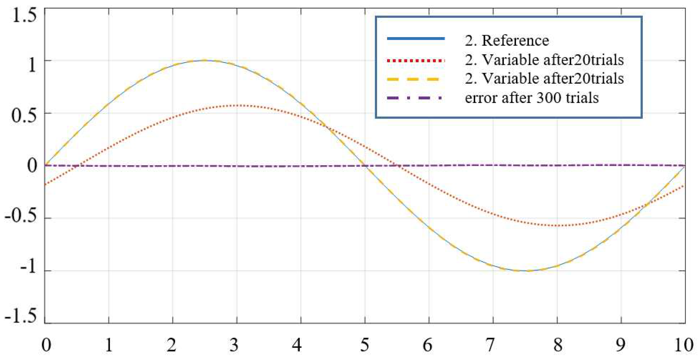
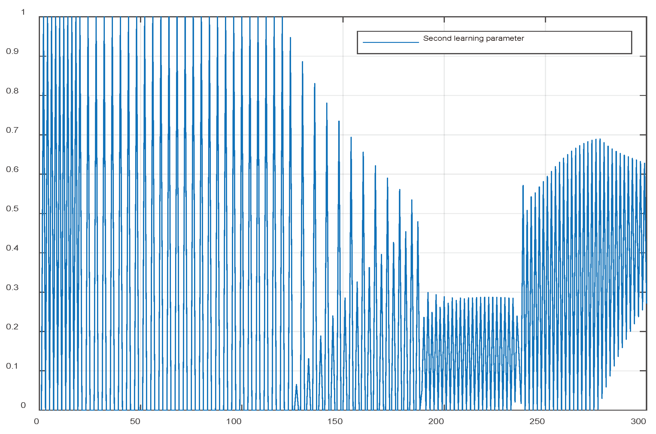
For "Smart" determination, the learning function parameter is

K_{k} = d i a g (K_{k}^{(j)}), j = 1, 2, ..., n

the input/output signal pair index

u_{j} \mapsto q_{j}

. This result shows that the controller has provided the required tracking quality, and after 300 trials, the output signal has tracked the password set in both channels.

When using formula (40) to determine the intelligent learning parameter in the iterative learning controller instead of (39), the quality of tracking the set signal is unchanged. The difference now is only the appropriate change. The results of the two learning parameters

K_{k}^{1}, K_{k}^{2}

are shown in Figure 14, Figure 15, Figure 16, and Figure 17.

7. Conclusions

Propose a two-loop control structure for the robot, in which the inner loop is an uncertain function component estimator to compensate for the robot's input, and the outer circle is an iterative learning controller (Figure 2). The Taylor series analysis method was used to create an inner loop controller. This method does not necessitate the creation of a mathematical model of the robot. For estimating, it simply takes measured signal values from previous systems. Develop two options for installing an iterative learning controller in the outer loop. The difference between these two options lies in the online determination of learning function parameters. The two proposed control circuits have been installed into the control algorithm and simulated with the planar robot to evaluate the quality. The correctness of the above-mentioned solutions has been demonstrated by theory and validated by simulation - Create a control algorithm based on the concepts above for controlling two items that work in batch processes in industry robots. These control algorithms are all distinguished because they do not (or only very infrequently) employ the mathematical model of the control object. The quality of these control algorithms has also been verified through a 2-DOF robot simulation. However, there are still disadvantages when building methods to determine convergence parameter sets for nonlinear learning functions with known structures. The problem of constrained control by iterative learning still needs to be solved. These will be the following research directions.

References

L.Lewis, D.M. L.Lewis, D.M. Dawson and C.T.Abdallah, “ Robot manipulator control theory and practice”, Marcel Dekker, 2004.
W. Spong, S. W. Spong, S. Hutchinson, and M. Vidyasagar,” Rovot modeling and control”, New York, Wiley, 2006.
Z. S. Jiang, F. Z. S. Jiang, F. Xei, X. Wang anf Z. Li, “Adaptive dynamic sliding mode control for space manipulator with external disturbance”, Journal of Control and, 2019.
Goel, A Swarup, “MIMO uncertain nonlinear system control via adaptive hight-order super twisting sliding mode and its application to robotic manipulator”, Journal Control Autom. Electr. Syst., 28, 36-49, 2017.
Wang, Y et.al.; “Servy on iterative leaning control, repetitive control and run to run control. Journal of process control”, 19, (10), 589-1600, 2009.
R. Lee, L. R. Lee, L. Sun, Z. Wang, M.Tomizuka,” AdaptivebILCcontrol of robot manipulators for friction compensation”. IFAC PapersOnline 52 (15), 175-180, 2019.
F. Boiakrif, D. F. Boiakrif, D.Boukhetala and F.Boudjema Velocity observer-based ILCcontrol for robot manipulators. F Bouakrif, D Boukhetala, F Boudjema. International Journal of Systems Science 44 (2), 214,222, 2013.
Nguyen, P.D.; Nguyen, N.H. Adaptive control for nonlinear non-autonomous systems with unknown input disturbance. Int. J. Control. 2021, 95, 3416–3426. [Google Scholar] [CrossRef]
Jeyasenthil, R.; Choi, S.-B. A Robust Controller for Multivariable Model Matching System Utilizing a Quantitative Feedback Theory: Application to Magnetic Levitation. Appl. Sci. 2019, 9, 1753. [Google Scholar] [CrossRef]
Nguyen, P.D.; Nguyen, N.H. Adaptive control for nonlinear non-autonomous systems with unknown input disturbance. Int. J. Control. 2021, 95, 3416–3426. [Google Scholar] [CrossRef]
K. G. Tran, N. H. K. G. Tran, N. H. Nguyen, P. D. Nguyen “Observer based controller two - wheeled inverted robots with unknown input disturbance and model uncertainty”, Journal of Control Science and Engineering, 1-12, 2020.
Husnain, S.; Abdulkader, R. Fractional Order Modeling and Control of an Articulated Robotic Arm. Eng. Technol. Appl. Sci. Res. 2023, 13, 12026–12032. [Google Scholar] [CrossRef]
Zouari, L.; Chtourou, S.; Ben Ayed, M.; Alshaya, S.A. A Comparative Study of Computer-Aided Engineering Techniques for Robot Arm Applications. Eng. Technol. Appl. Sci. Res. 2020, 10, 6526–6532. [Google Scholar] [CrossRef]
Ben Ayed, M.; Zouari, L.; Abid, M. Software In the Loop Simulation for Robot Manipulators. Eng. Technol. Appl. Sci. Res. 2017, 7, 2017–2021. [Google Scholar] [CrossRef]
Duc, D.M.; Tuy, T.X.; Phuoc, P.D. A Study on the Response of the Rehabilitation Lower Device using Sliding Mode Controller. Eng. Technol. Appl. Sci. Res. 2021, 11, 7446–7451. [Google Scholar] [CrossRef]

Figure 1. Two -DOF planar robot arm.

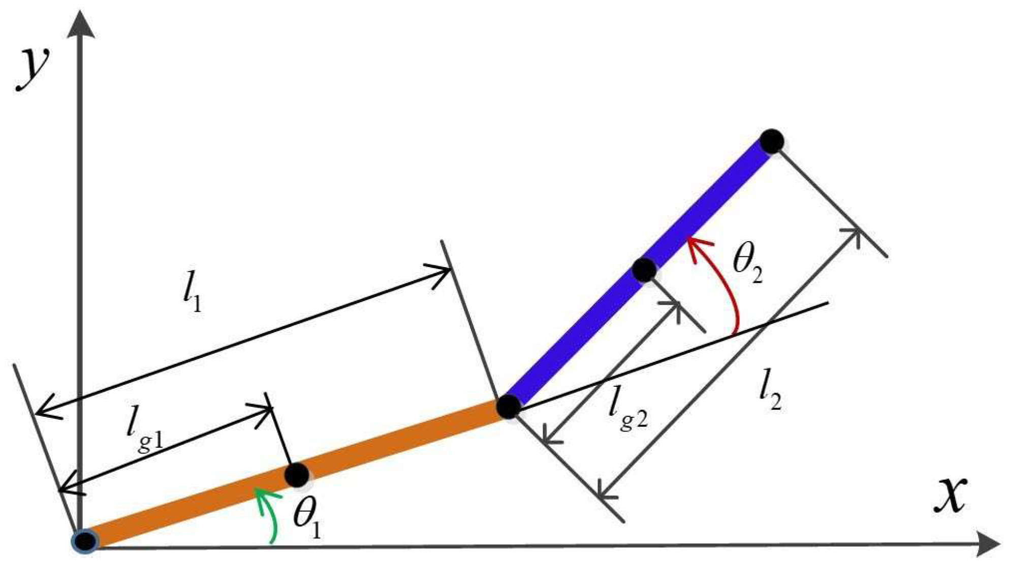
Figure 2. Structure the first diagram for robot control using the iterative learning method.

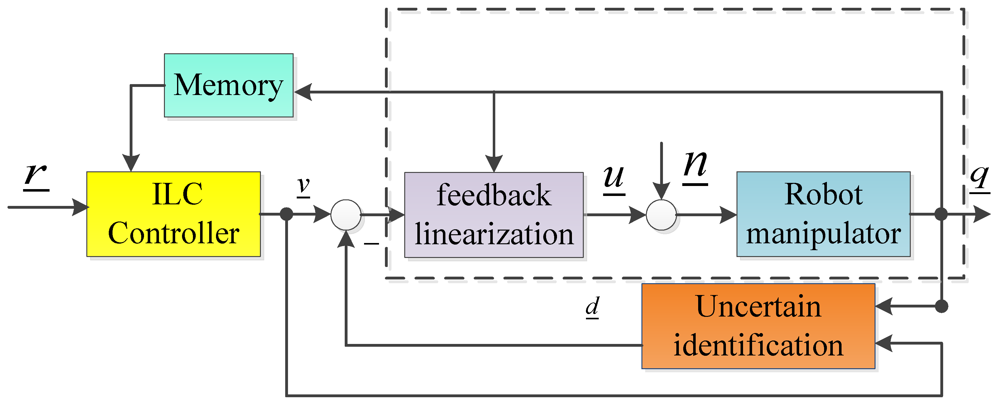
Figure 3. Structure the second diagram for robot control using the iterative learning method.

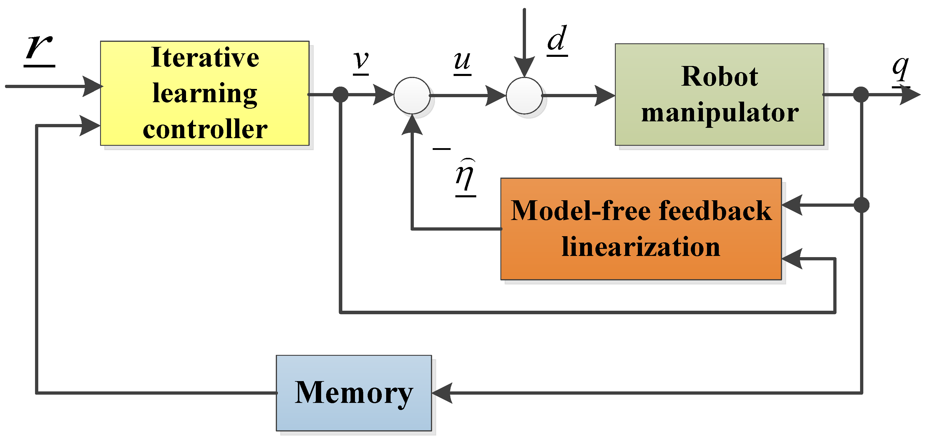
Figure 4. Output tracking results after 20 trials of the first joint.

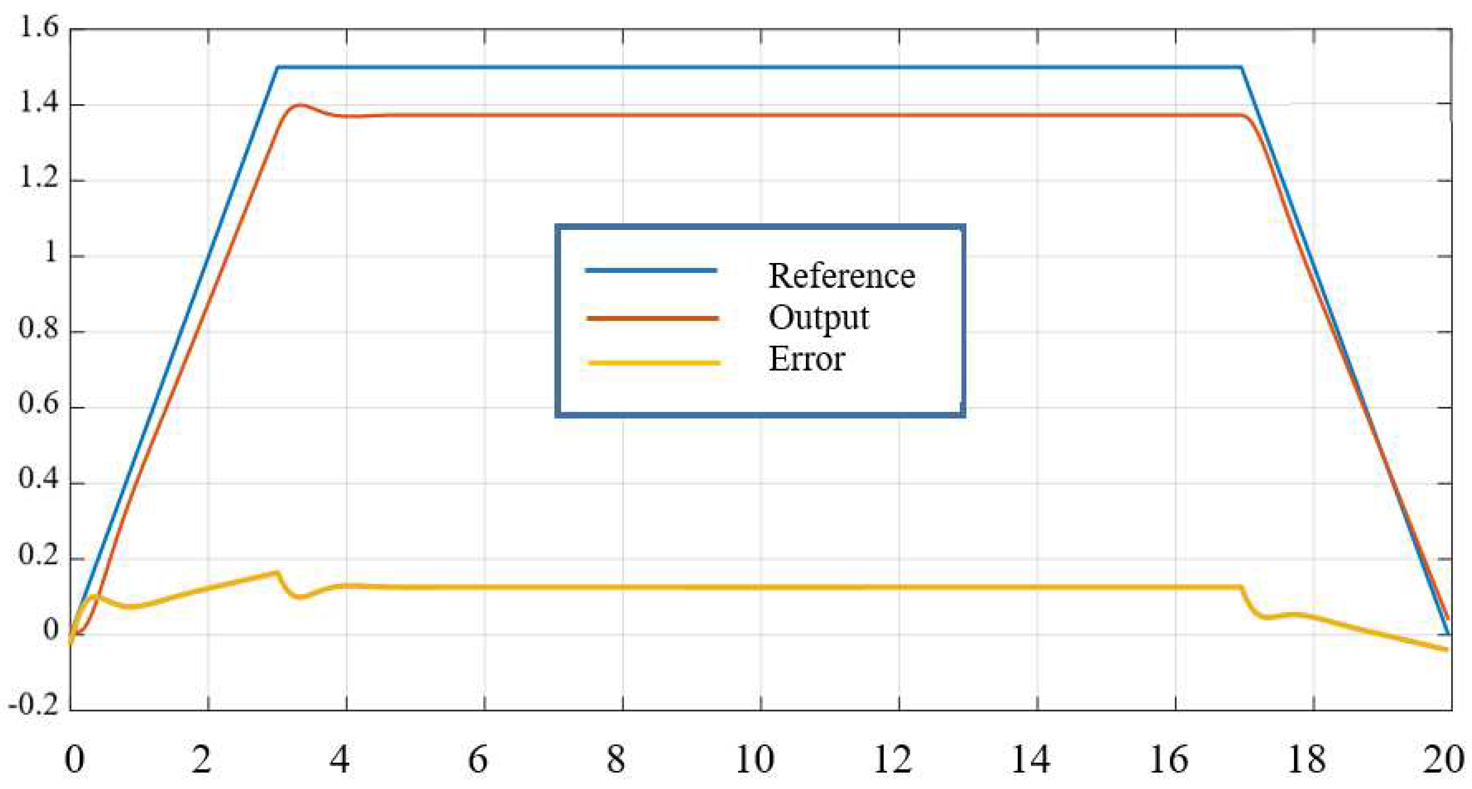
Figure 5. Output tracking results after 20 trials of the second joint.

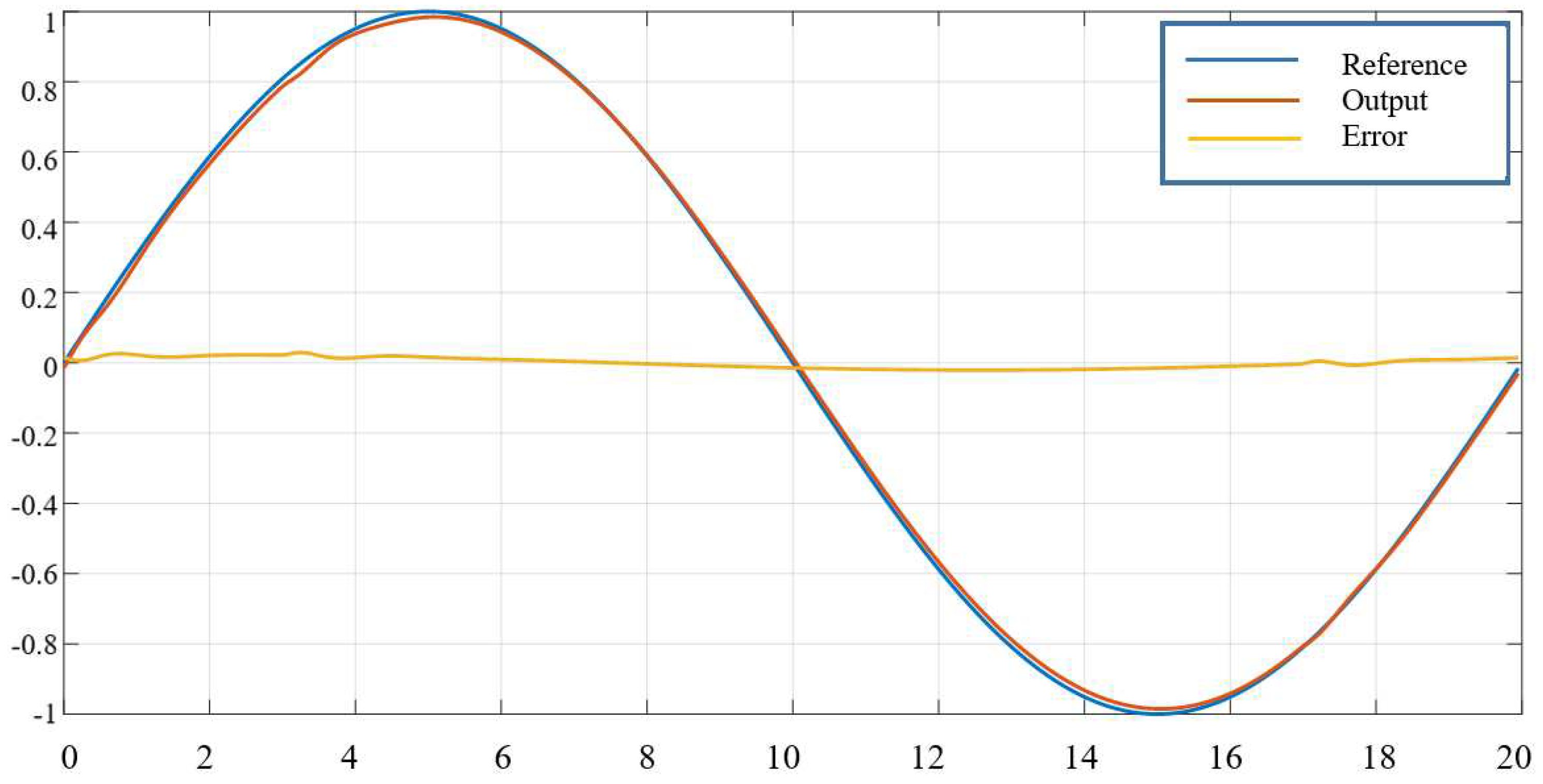
Figure 6. Output tracking results after 60 trials of the first joint.

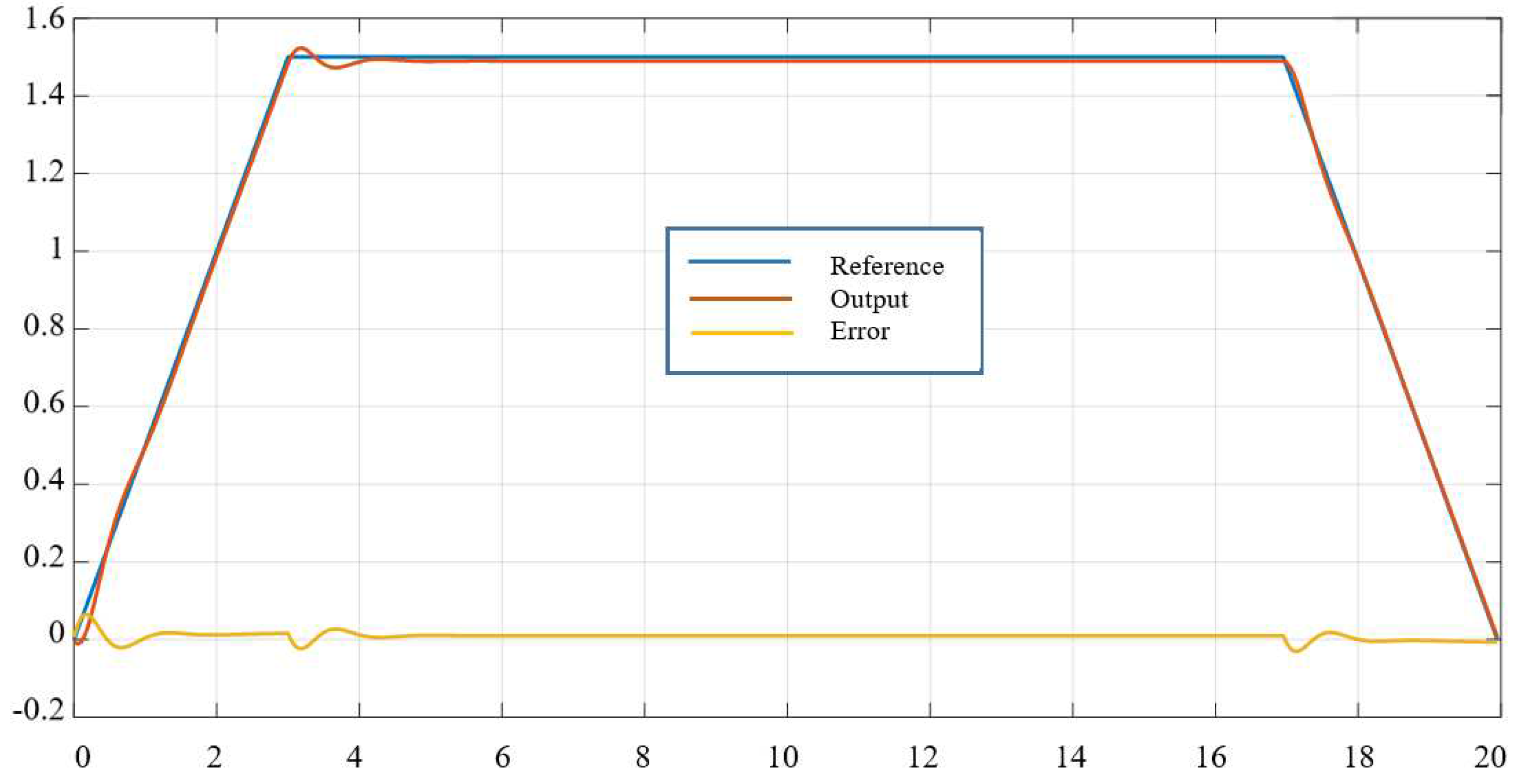
Figure 7. Output tracking results after 60 trials of the second joint.

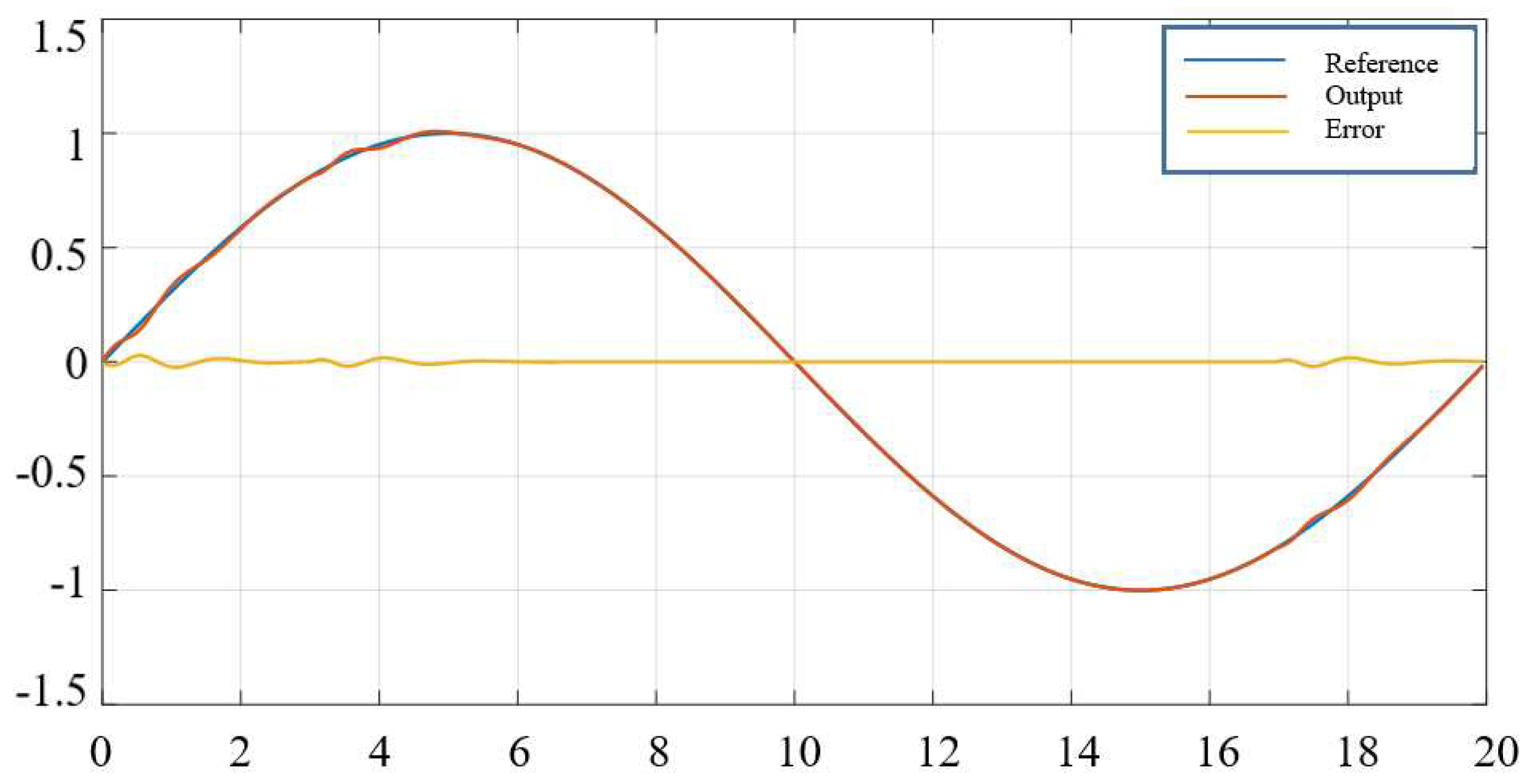
Figure 8. The output response of the first common variable after trying 15 and 250 times.

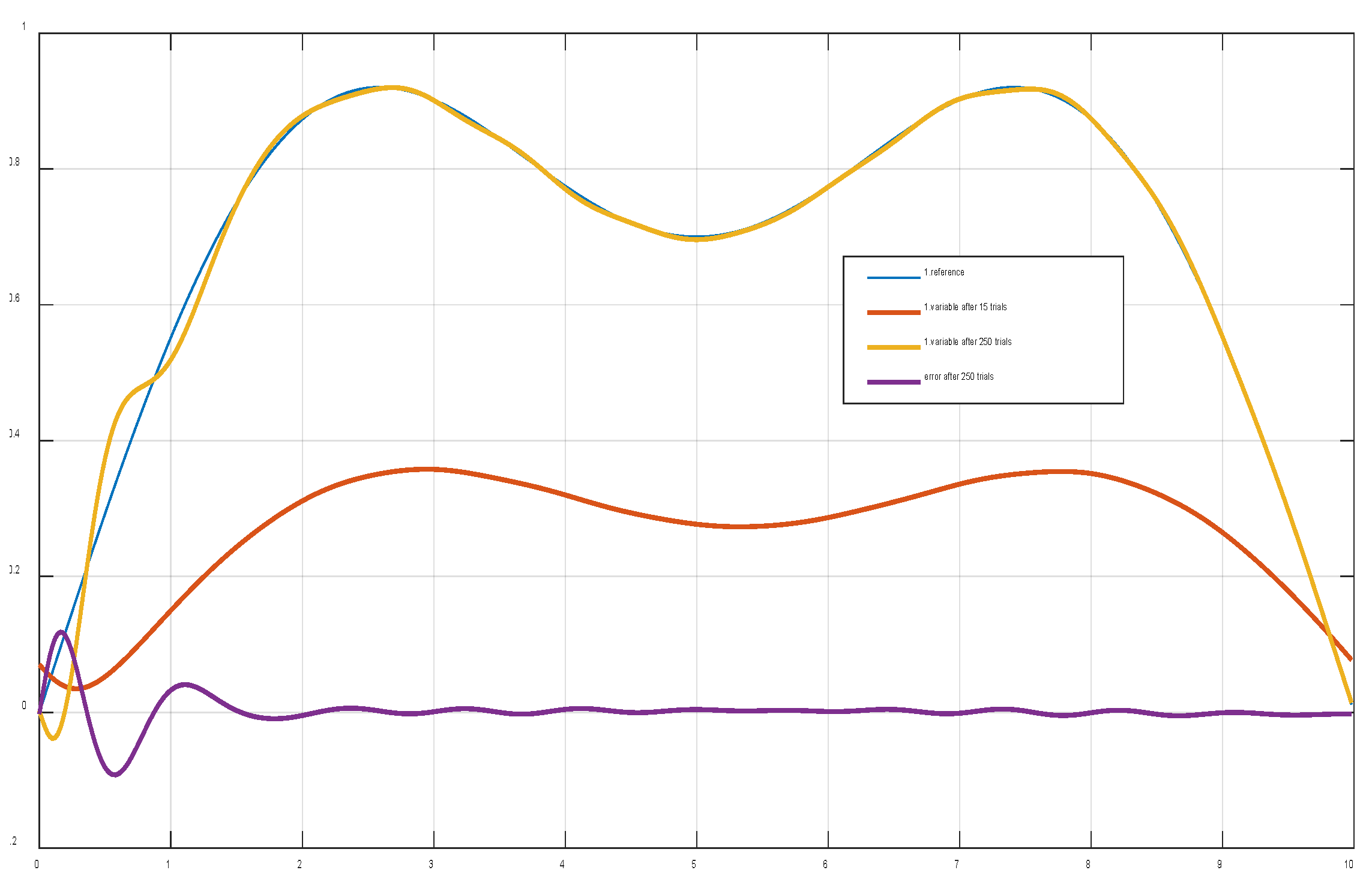
Figure 9. The output response of the second common variable after trying 15 and 250 times.

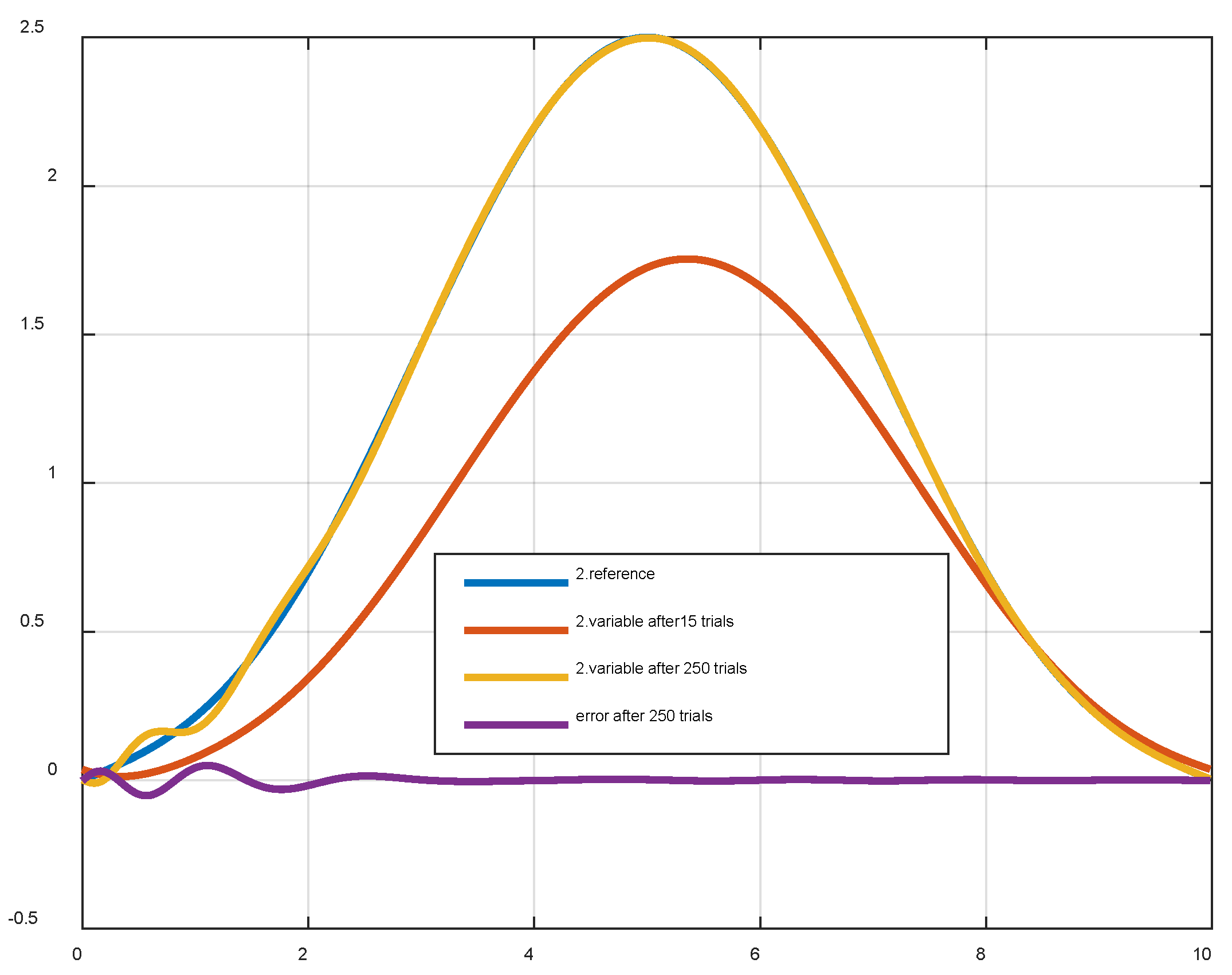
Figure 10. Meets the position of the first joint when used (39).

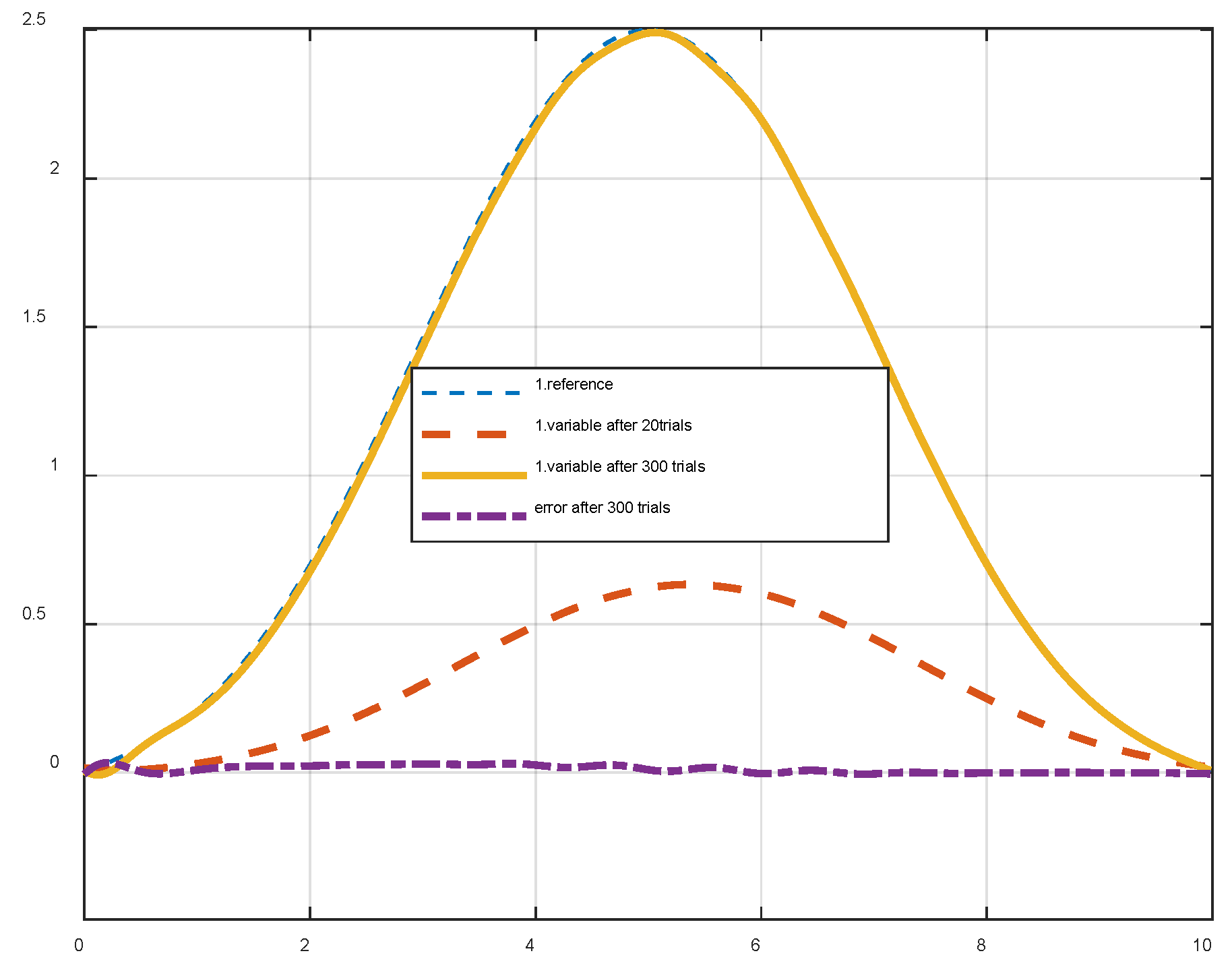
Figure 11. Meets the position of the second joint when used (39).

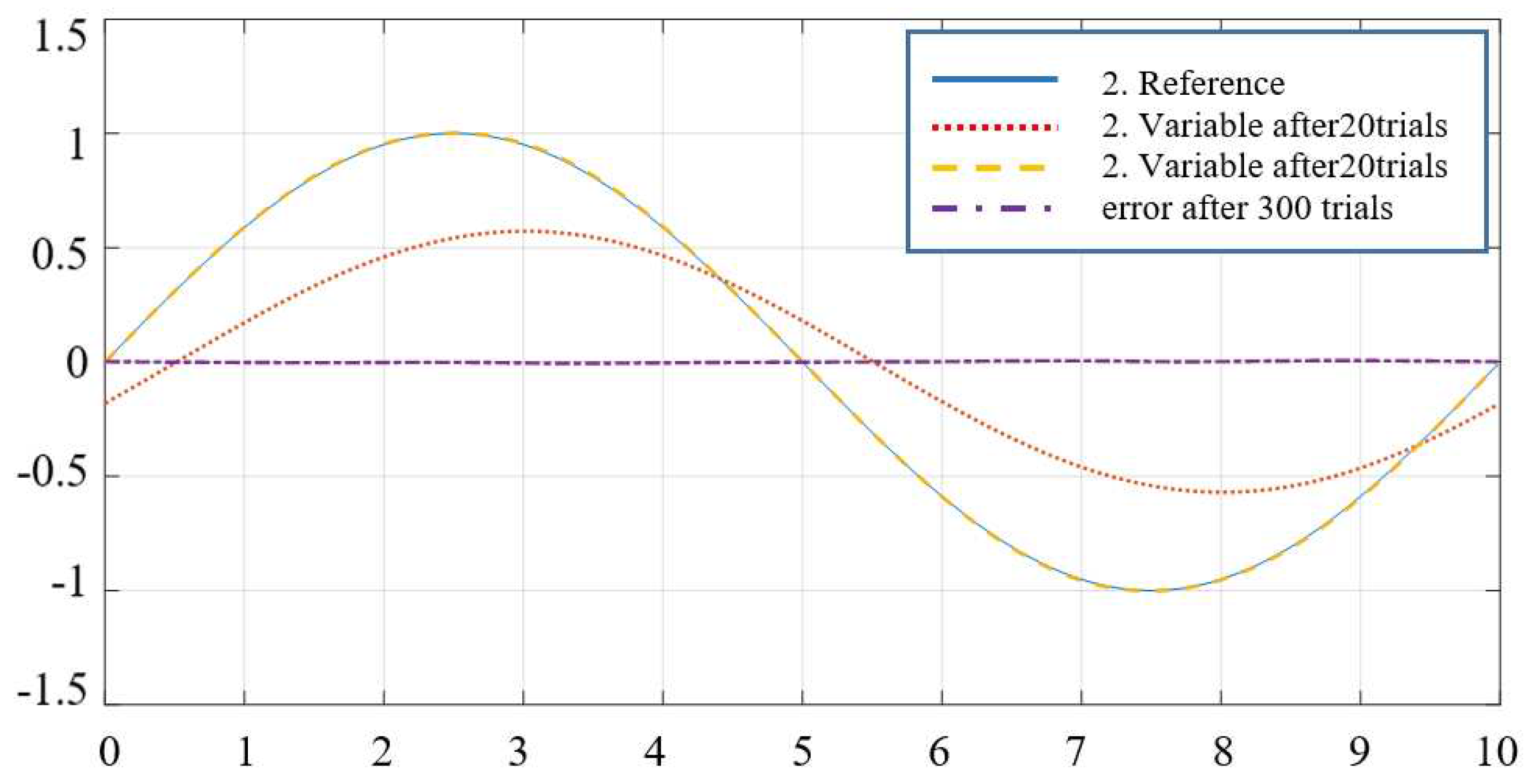
Figure 12. Meets the position of the first joint when used (40).

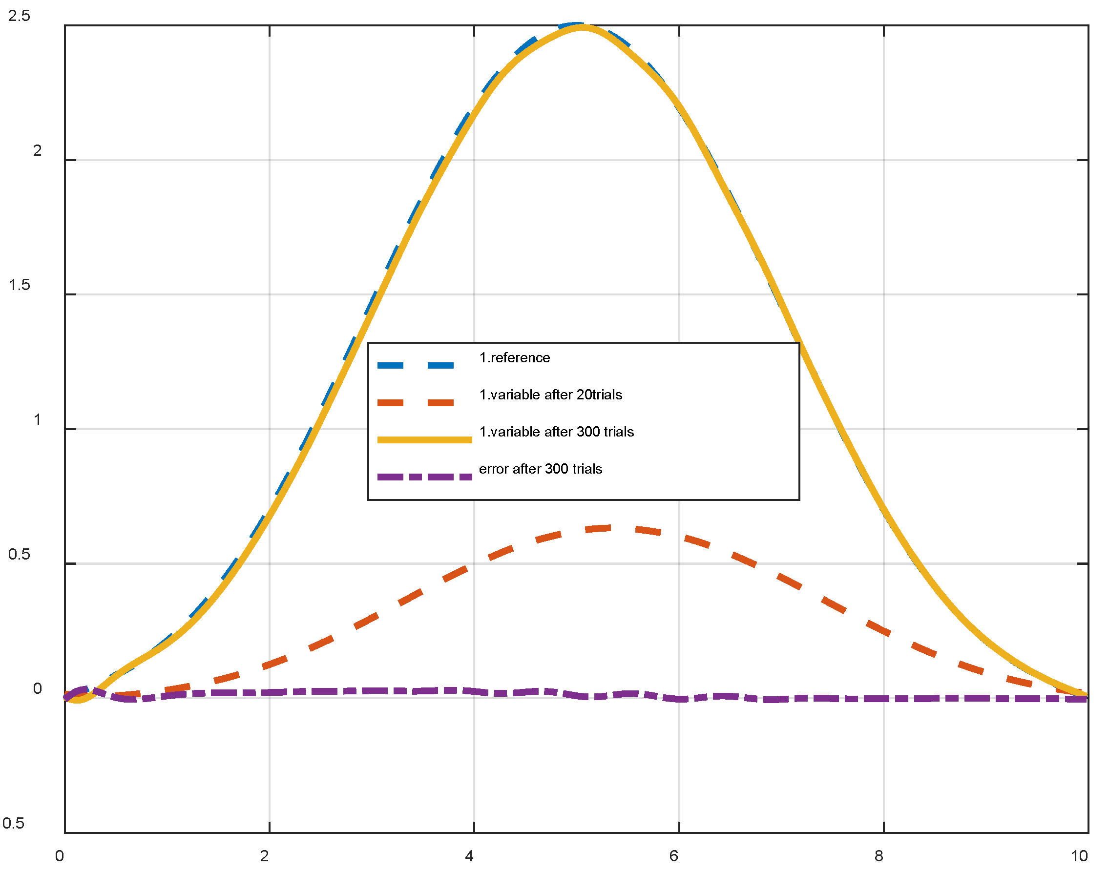
Figure 14. Change in the first learning function parameter when using (39).

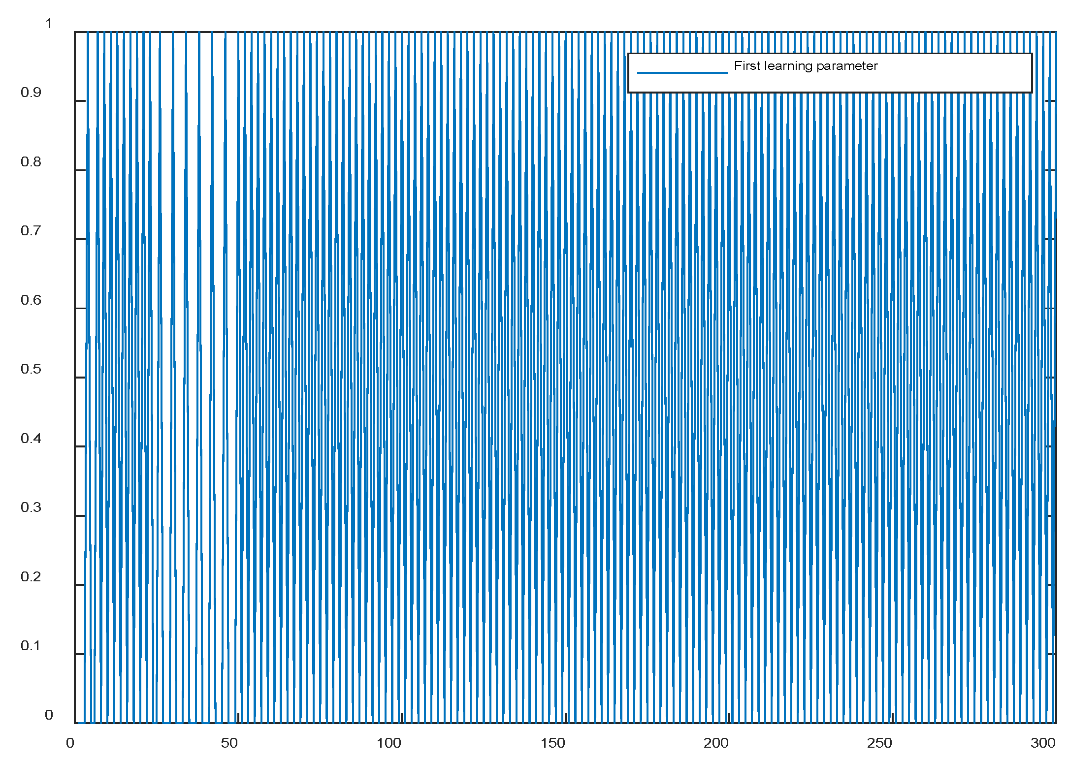
Figure 15. Change in the second learning function parameter when using (39).

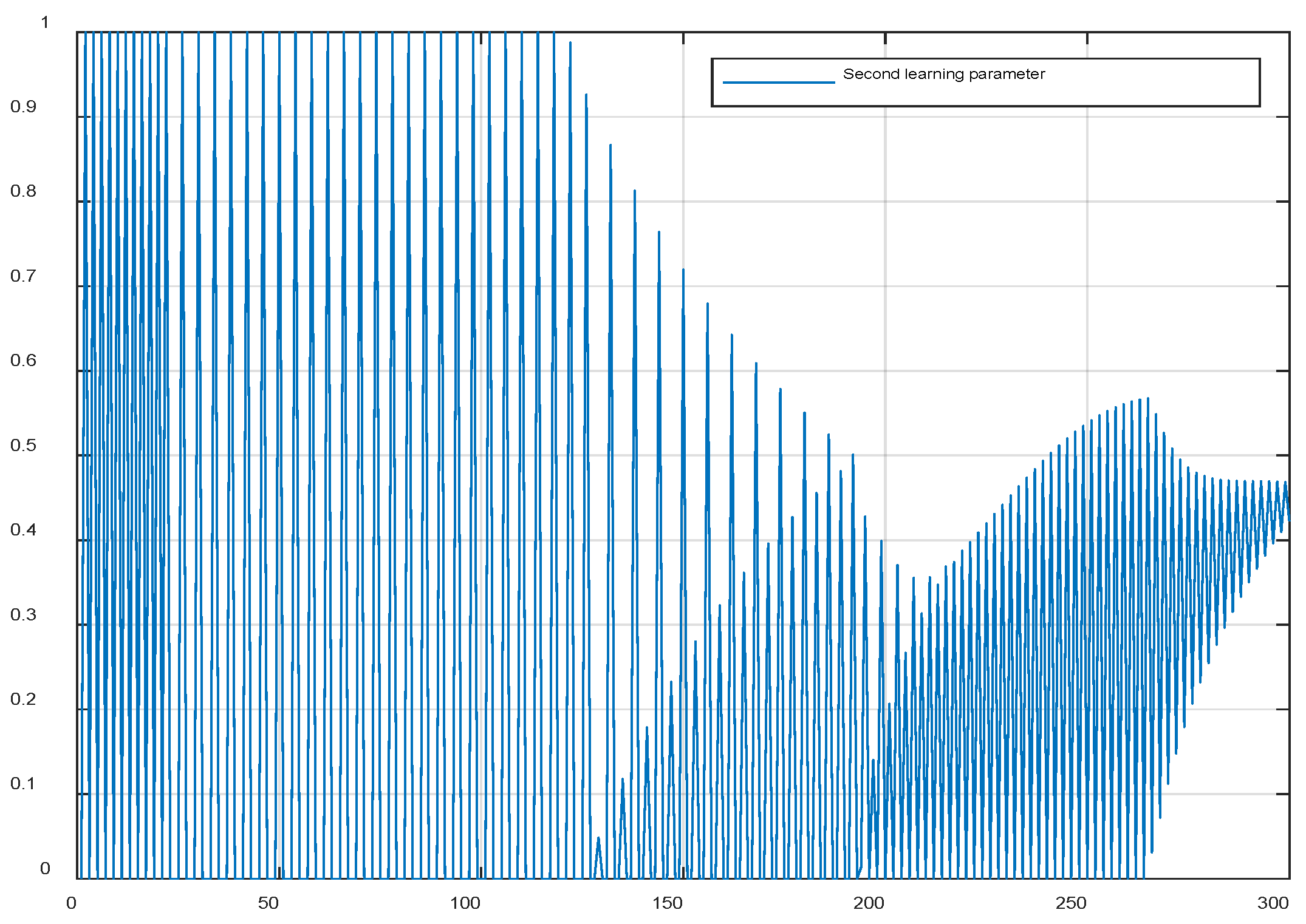
Figure 16. Change in the first learning function parameter when using (40).

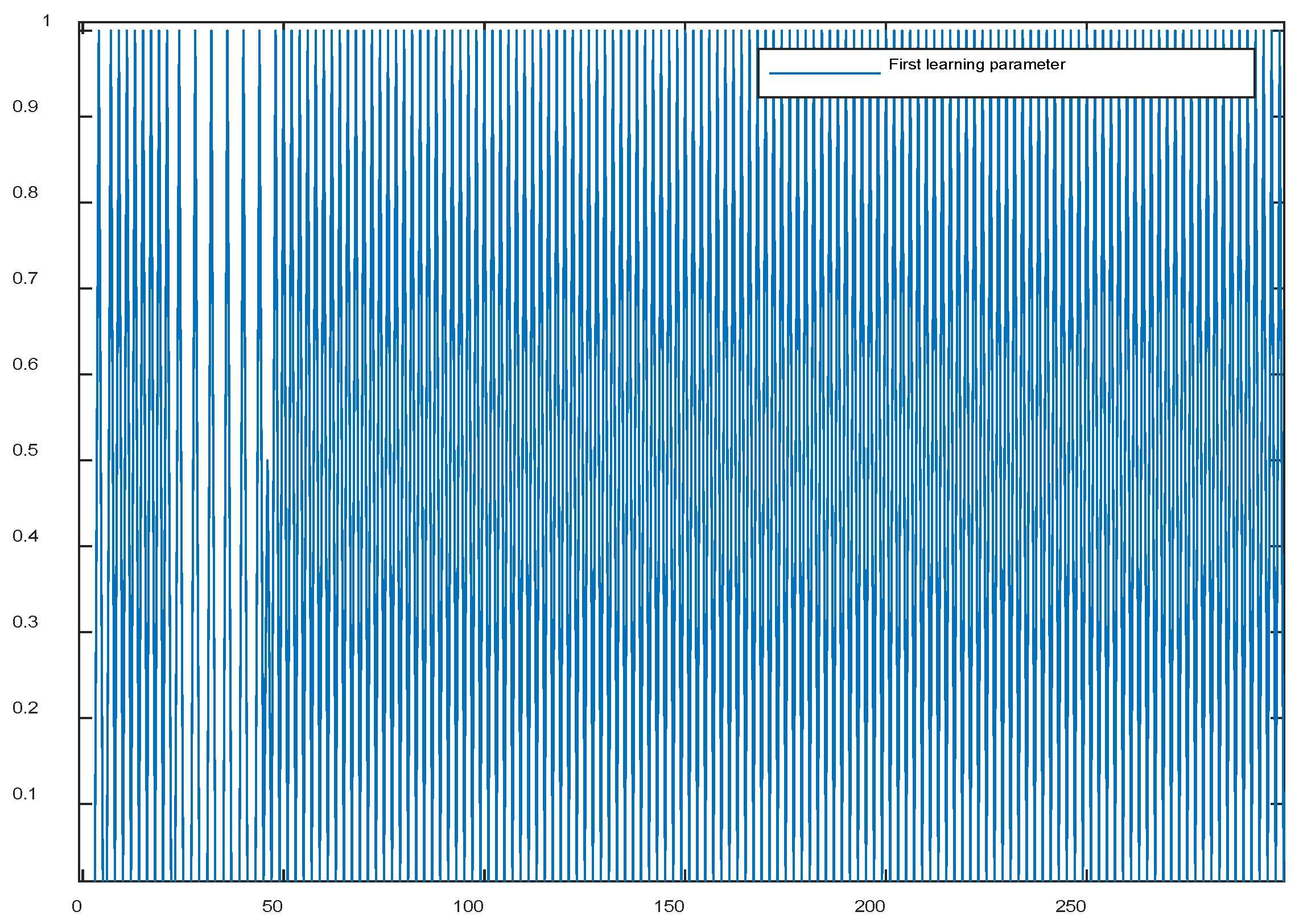
Figure 17. Figure 17. Change in the second learning function parameter when using (40).

Disclaimer/Publisher’s Note: The statements, opinions and data contained in all publications are solely those of the individual author(s) and contributor(s) and not of MDPI and/or the editor(s). MDPI and/or the editor(s) disclaim responsibility for any injury to people or property resulting from any ideas, methods, instructions or products referred to in the content.

© 2024 by the authors. Licensee MDPI, Basel, Switzerland. This article is an open access article distributed under the terms and conditions of the Creative Commons Attribution (CC BY) license (http://creativecommons.org/licenses/by/4.0/).

Copyright: This open access article is published under a Creative Commons CC BY 4.0 license, which permit the free download, distribution, and reuse, provided that the author and preprint are cited in any reuse.

MDPI Initiatives

Important Links

Choose an area of interest and we will send you notifications of new preprints at your preferred frequency.

Disclaimer

Improve the quality of Industrial Robot Control Using an Iterative Learning Method with Online Optimal Learning and Intelligent Online Learning Function Parameters

Abstract

1. Introduction

2. Robot planar dynamic model

3. Two structure diagrams for robot control using iterative learning method

4. Structure the first diagram for robot control the iterative learning method

4.1. Algorithm content according to the first control diagram

4.2. Applied to robot control

5. The structure of the second iterative learning controller with model-free determination of optimal learning parameters for industrial robot

5.1. Algorithm content according to the first control diagram

5.2. Feedback linearization for internal loop control using model-free disturbance compensation

5.3. Outer loop control is by iterative learning controller design.

5.4. Control algorithm and performance of closed – loop system

5.5. Applied to robot control

6. The structure of the second iterative learning controller with model-free determination of online learning parameters for industrial robot

6.1. Control the inner loop

6.2. Outer loop control is by iterative learning controller design.

6.3. Applied to robot control

7. Conclusions

References

MDPI Initiatives

Important Links

Subscribe