1. INTRODUCTION
Nanoindention is especially used for the determination of mechanical properties on a very small scale applicable to thin films and nanostructures and has been used by us over the last few years [
1,
2,
3,
4,
5,
6,
7,
8,
9,
10,
11].. It is based upon load-depth (P-h) plots, which many researchers tried to generalize. Among them P=αh
m is the most popular equation and it is given by Oliver and Pharr. Based on which many other unloading curves are proposed. We are however considering the loading and unloading curves previously proposed [
12] as per the elastic-plastic nature of the sample, which are given by
eq 1 (a, b-d) for loading (same for all the cases) and unloading (differing as per the sample nature) portions.
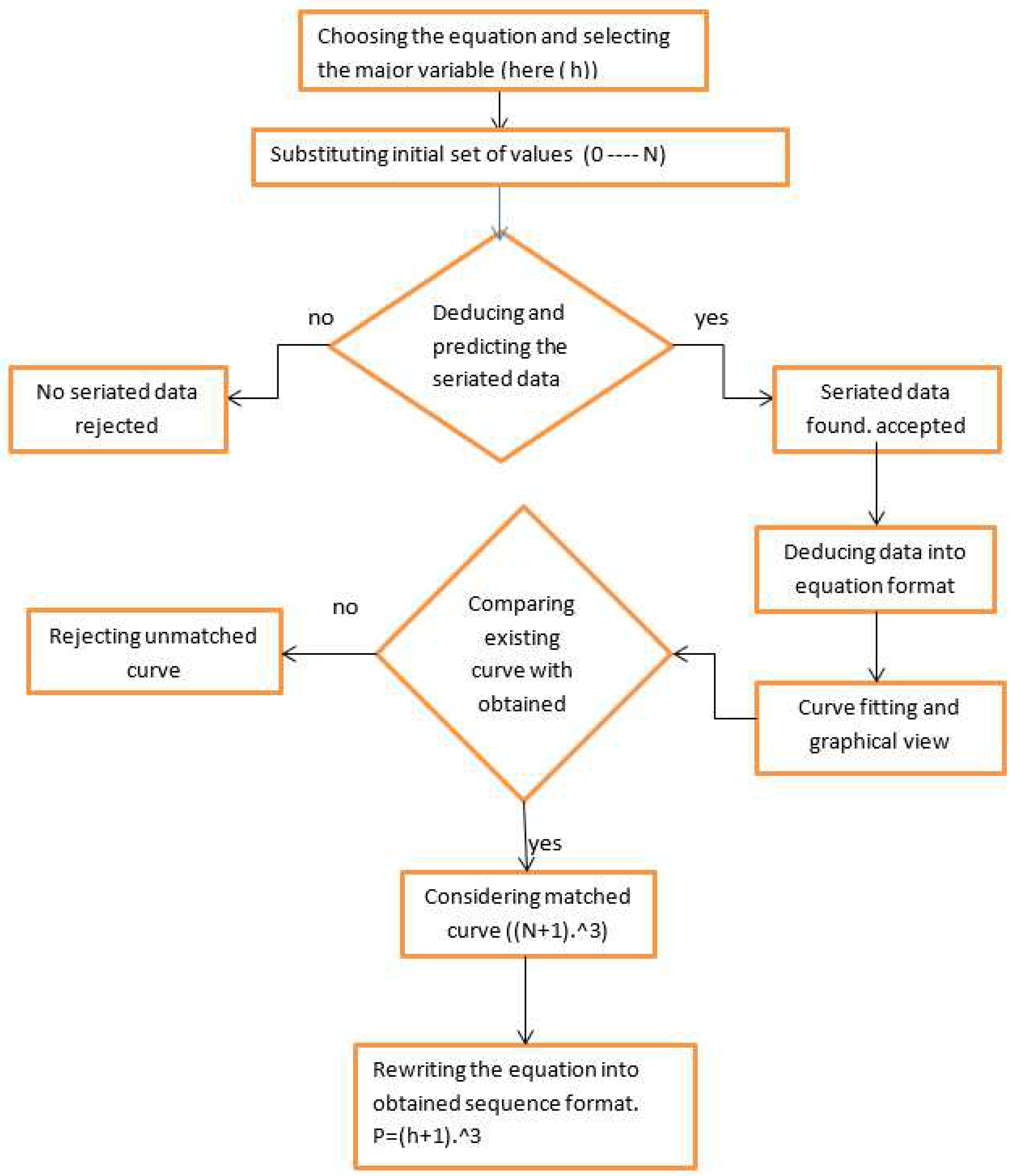
The method of substituting the original value is not novel. By setting all of the variables to unity, we can typically utilize this strategy to find a constant in an equation. The idea is the same, but we will consider a starting collection of values, say from 0 (zero) to N (in this case, N=10), rather than taking a single value of unity. Moreover, we attempt to infer the fundamental value (in this example, "h") from that equation rather of looking for a constant. We could view it as a novel algorithmic technique.. The flow chart diagram for algorithm as shown below (
Figure 1).
2. Obtaining loading and unloading curve equations:
The following calculations were made to estimate all possible loading and unloading curves substituting initial values (or general values) in the existing curves. By substituting process possibly, we would get the fallowing equations:
For loading: (i) h.^3 and (ii) (h+1).^3 and
For unloading: (i)2.*h (ii)h+2 (iii)(2.*h)-1
{these were to be included to get the unloading curve}
2.1. Calculating Loading curves:
Let us assume m=2 and n and h values starts from 1 to n but for the instant n=1 to 0;and h=1 to 10;
Then we will get P values as sown below:
| 1 |
8 |
27 |
64 |
125 |
216 |
343 |
512 |
729 |
1000 |
From above data, we can rewrite tabular content as
(1.^3),(2^3),(3^3),(4^3),(5^3),(6^3),(7^3),(8^3),(9^3),(10^3)………..
(or)
((1+0).^3),((1+1)^3),((2+1)^3),((3+1)^3),((4+1)^3),((5+1)^3),((6+1)^3),((7+1)^3),((8+1)^3)((9+1)^3)…………
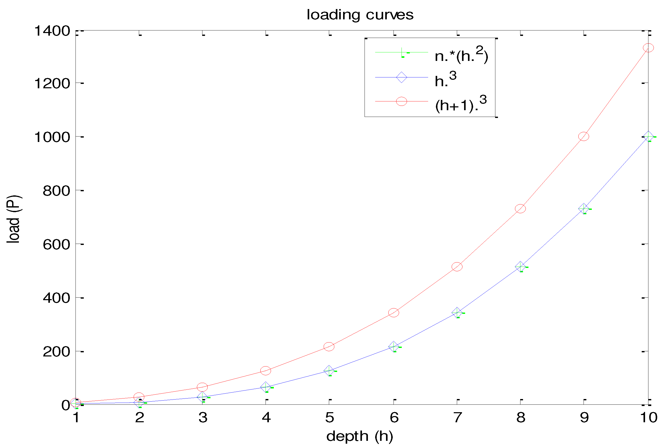
By generalizing the above sequences we can write (h.^3) and ((h+1).^3). Hence, the possible loading curve equations can be represented as
eq 2 a, b. The graphical representation is as given below, the structure of all curves seems to be similar and red curve indicates ((h+1).^3) and other two curves were merged (i.e., n.*(h.^3) and h.^3) (
Figure 2).
2.2. Calculating Unloading curves:
The same considerations were also made like loading curve calculations. Let us assume m=2 and n and h values starts from 1 to n but for the instant n=1 to 10 and h=1 to 10;. As there are four types of unloading curves (eq 1) by substituting the initial values in the respective variables, we would get the output values as follows: constant m=2
- a)
-
P1=[ n.*(h.^2)]-[n.*(max(h)-h).^(1/2)]
{(0) (2.0840) (4.0890) (5.9278) (7.7212) (9.4963) (11.2639) (13.0311) (14.8092)}
- b)
-
P2=[ n.*(h.^2)]-[(n.^2).*(max(h)-h).^(1/2)]
{(0.0000 + 0.0000i) (0.0000 + 1.1462i) (2.5499 + 0.0000i) (4.6497 + 0.0000i) (6.6551 + 0.0000i) (8.6546 + 0.0000i) (10.6831 + 0.0000i) (12.7813 + 0.0000i) (15.0502 + 0.0000i)}
- c)
-
P3=[ n.*(h.^2)]-[n.*(max(h)-h).^(5/2)]
{(0.0000 + 0.0000i) (0.0000 +10.5848i) (0.0000 + 2.8083i) (8.5556 + 0.0000i) (11.5853 + 0.0000i) (13.3607 + 0.0000i) (14.4873 + 0.0000i) (15.2599 + 0.0000i) (15.9140 + 0.0000i)}
- d)
-
P4=[ n.*(h.^2)]-[(n.^2).*(max(h)-h).^(3/2)]
{(0.0000 + 0.0000i) (0.0000 + 7.5173i) (0.0000 + 7.5613i) (0.0000 + 5.6097i) (4.0795 + 0.0000i) (9.0834 + 0.0000i) (12.6645 + 0.0000i) (15.5754 + 0.0000i) (17.8050 + 0.0000i)}
It is very difficult to deal with imaginary part calculation, so for the purpose of easy calculation’s we are eliminating imaginary part and on approximating the values we would obtain the values as follows:
- a)
-
P1=[ n.*(h.^2)]-[n.*(max(h)-h).^(1/2)]
0 2 4 6 8 …. (for series considerations)
- b)
-
P2=[ n.*(h.^m)]-[(n.^2).*(max(h)-h).^(1/2)]
3 5 7 9 11 13 15……(prime number series)
- c)
-
P3=[ n.*(h.^m)]-[n.*(max(h)-h).^(5/2)]
9 12 13 14 15 16……
- d)
-
P4=[ n.*(h.^m)]-[(n.^2).*(max(h)-h).^(3/2)]
4 9 13 16 19……
From the above results, we have two seriated equations and other two are not following any series. It is easy to deal with seriated data then no seriated data. So let us consider only two seriated data i.e.,
- a)
-
P1=[ n.*(h.^2)]-[n.*(max(h)-h).^(1/2)]
0 2 4 6 8 …. (2*N tabular series)
- b)
-
P2=[ n.*(h.^2)]-[(n.^2).*(max(h)-h).^(1/2)]
3 5 7 9 11 13 15……(prime number series)
From the above data, the data can be written in the form of series as n*2 and h+2 (or) (2.*h)-1. So our possible equations are as follows:
- i)
2.*h (3a)
- ii)
h+2 (3b)
- iii)
(2.*h)-1 (3c)
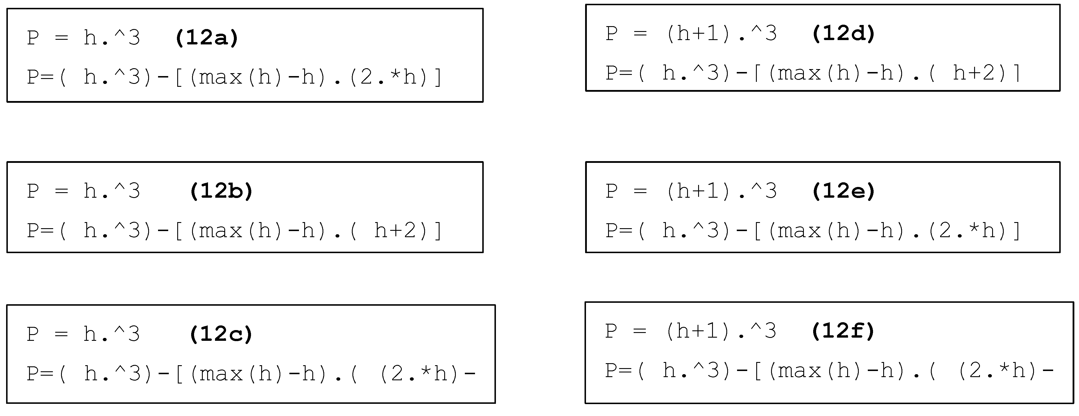
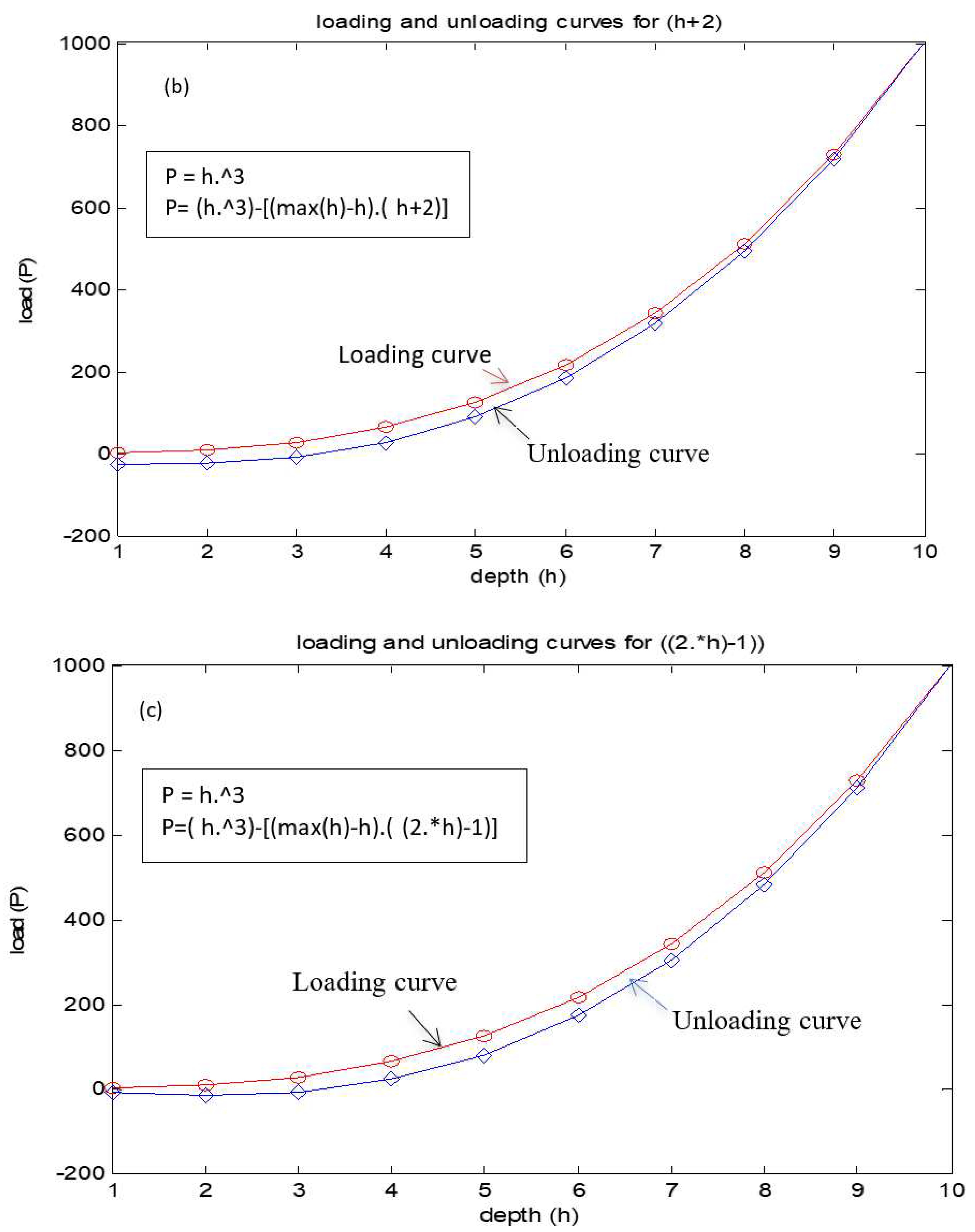
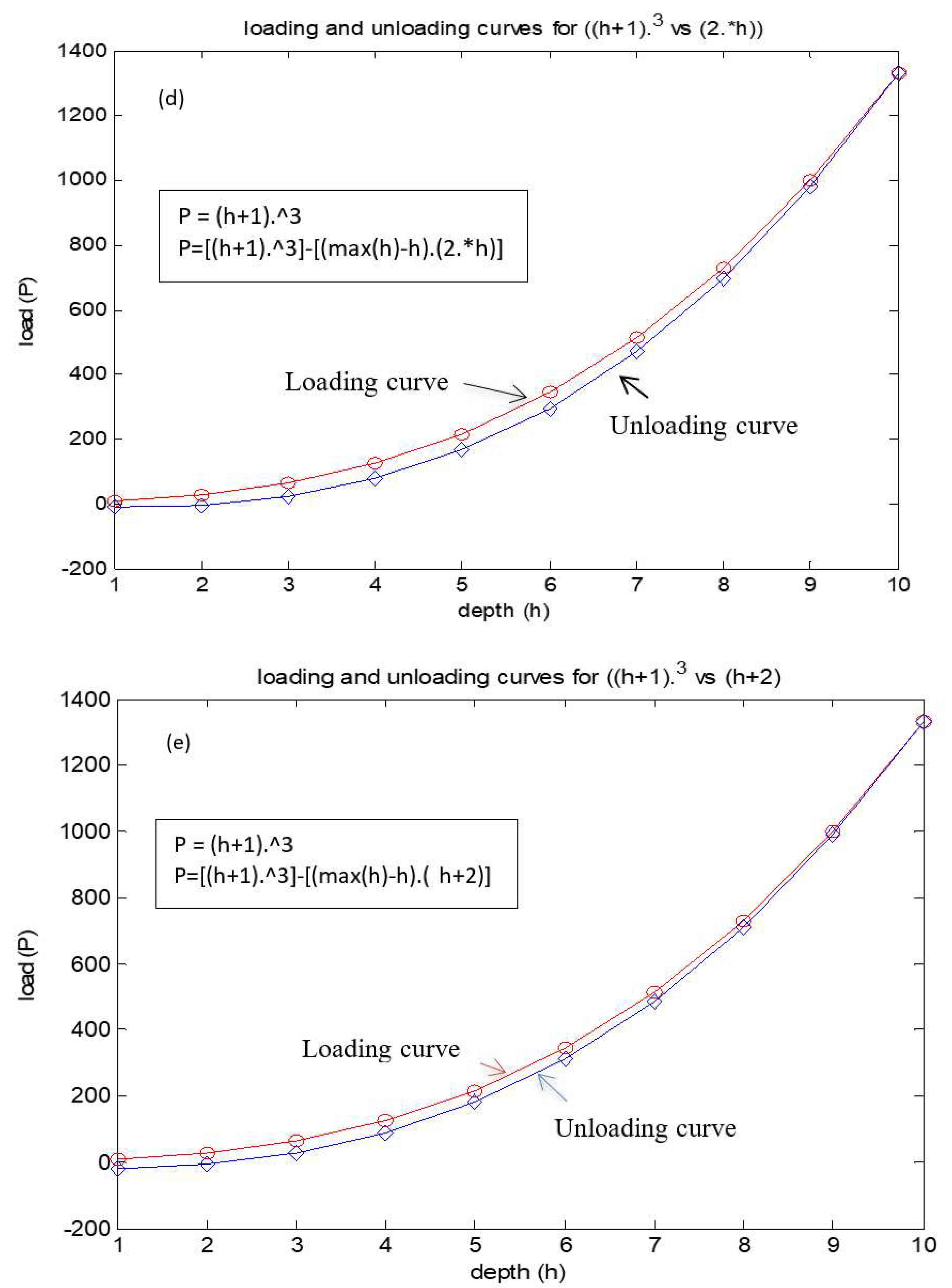
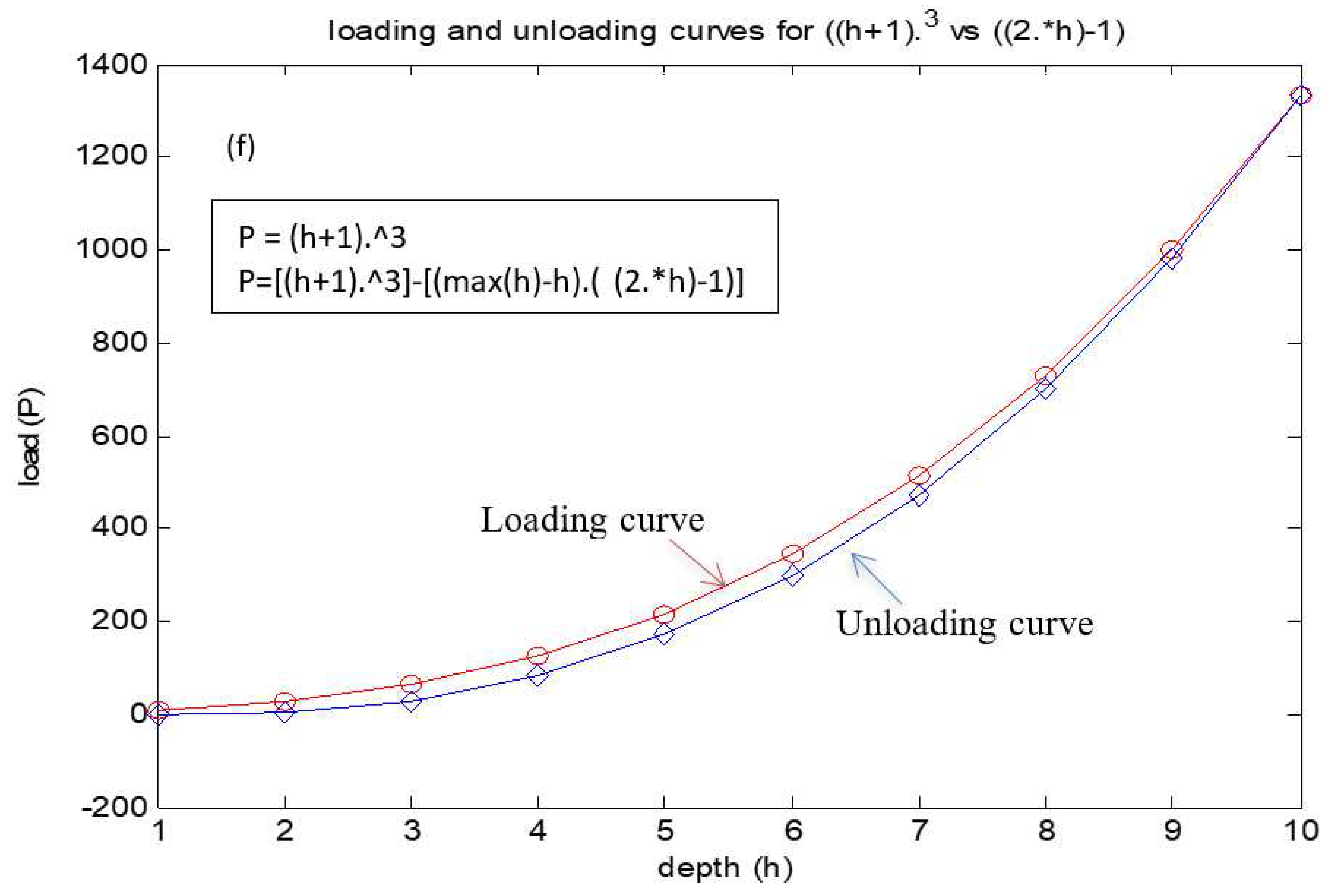
On considering all (loading and unloading) our possible equations we can have possible loading and unloading curve combinations would be six (2(loading)*3(unloading)). So the resultant equations are: (the bellow equations are loading and followed by its respective unloading equation).eq 4(a-f).
These are the possible equations which we obtained and their respective graphical representation is as shown below. The graphical representation of the equations is given by
Figure 3(a-f).
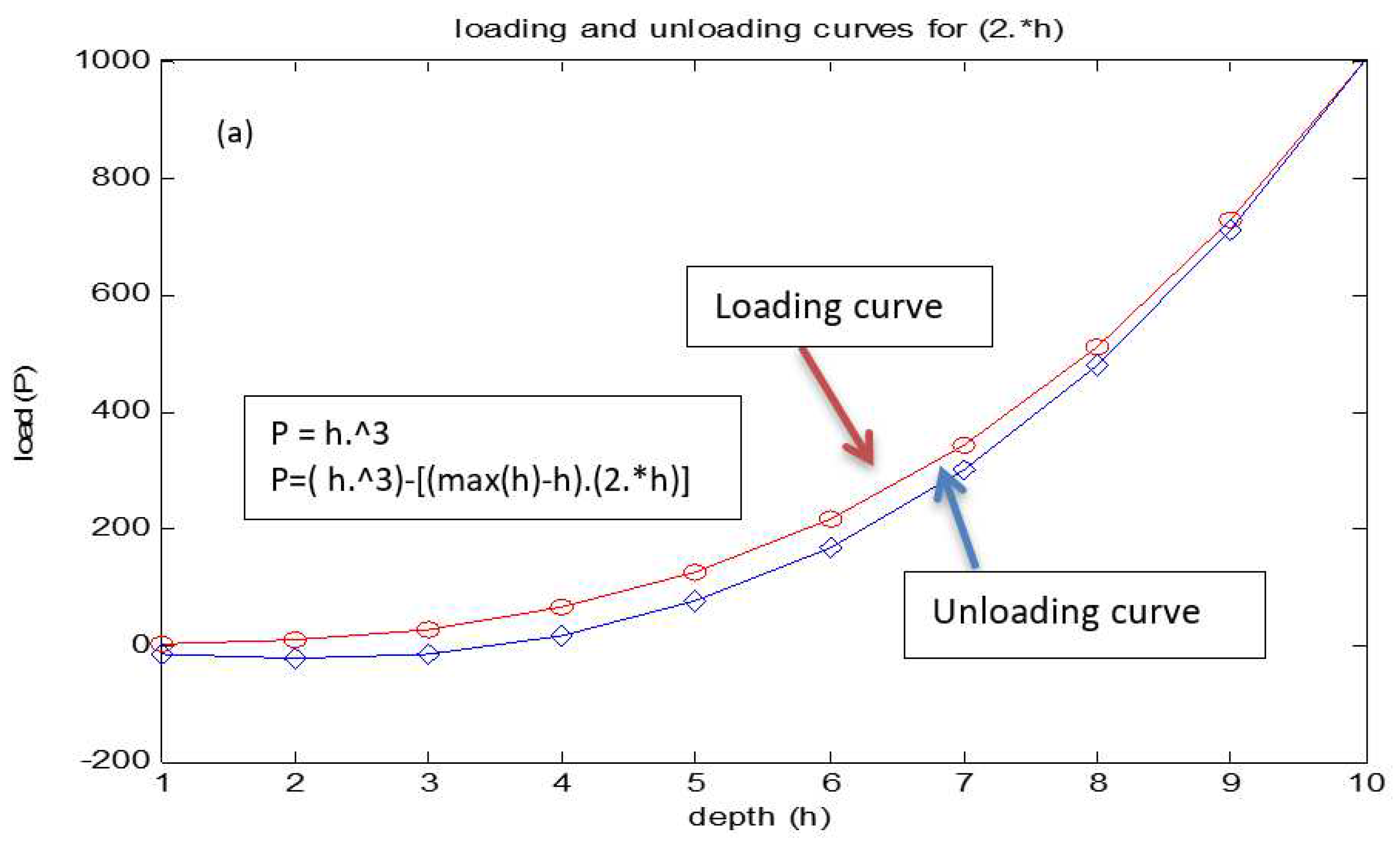
By observing above graphs, all unloading curves are not reaching the initial point (zero) except the last curve that is given by
So, on compression among all curves the above combination seems to be preferable. So, we will conclude it as result of our estimation and assumption. We can use these equations getting loading and unloading curves. So on conclusion we obtained loading and unloading curves as given below (
eq 5a, b) where “h” is replaced with “H”)
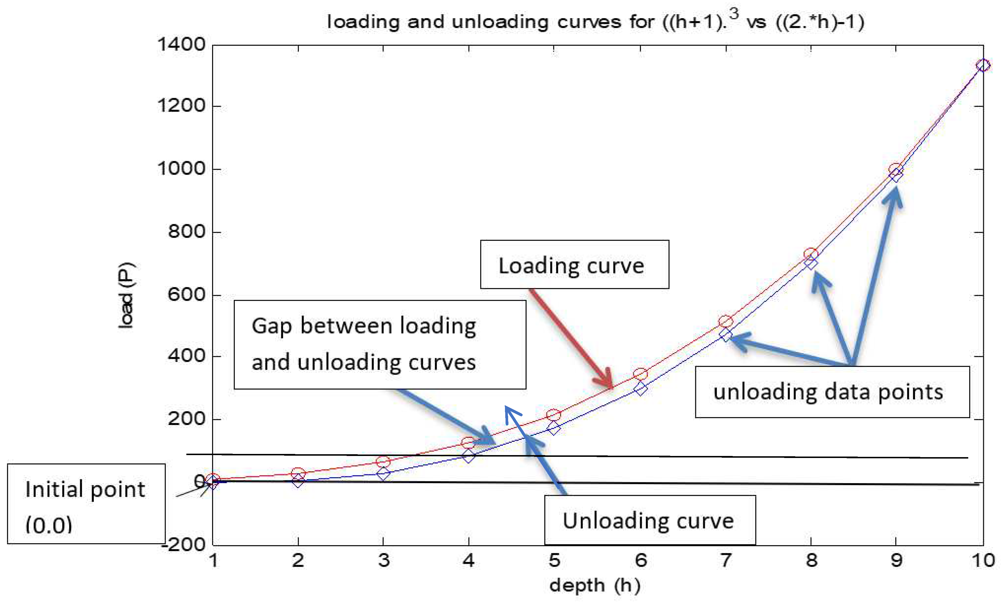
2.3. Description of curves:
In the curve, H denotes the depth values and P indicates the experienced load values with respective of depth. We were familiar with loading curve but we find difficulty in describing unloading curve. Here we try to describe the unloading curve. It includes three parts as the first part, to get the structure of downloading curve, second part to get the values for downloading curve and the last part is to maintain the gap between the loading and unloading curve, which we are going to discuss in the proceeding discussions (
Figure 4).
2.4. Advantage of proposed equations over existing equations:
[A]. The first target of making this communication is to eliminate the constant(s) values from the existing curve such as “n”, as we need these n values too, to get the plot in case of existing equation. Whereas in case of proposed equations, we need only loading (or) unloading data to establish the relation between them.
[B]. the curve proposed fits well with the Fibonacci series where the exiting curve fails, if the data fits with Fibonacci series. The Fibonacci series, generally given by
Fn=(fn-2) +( fn-1) and the series is
Fn=1,2,3,5,8,13,21,34,55,89………
2.5. Graphical representation for Fibonacci series with curves:
The graphical analysis is discussed below through curve fitting with Fibonacci seriated data for existing and proposed
eq (6a-e) and analyzed at end of all the graphical curve fitting. (
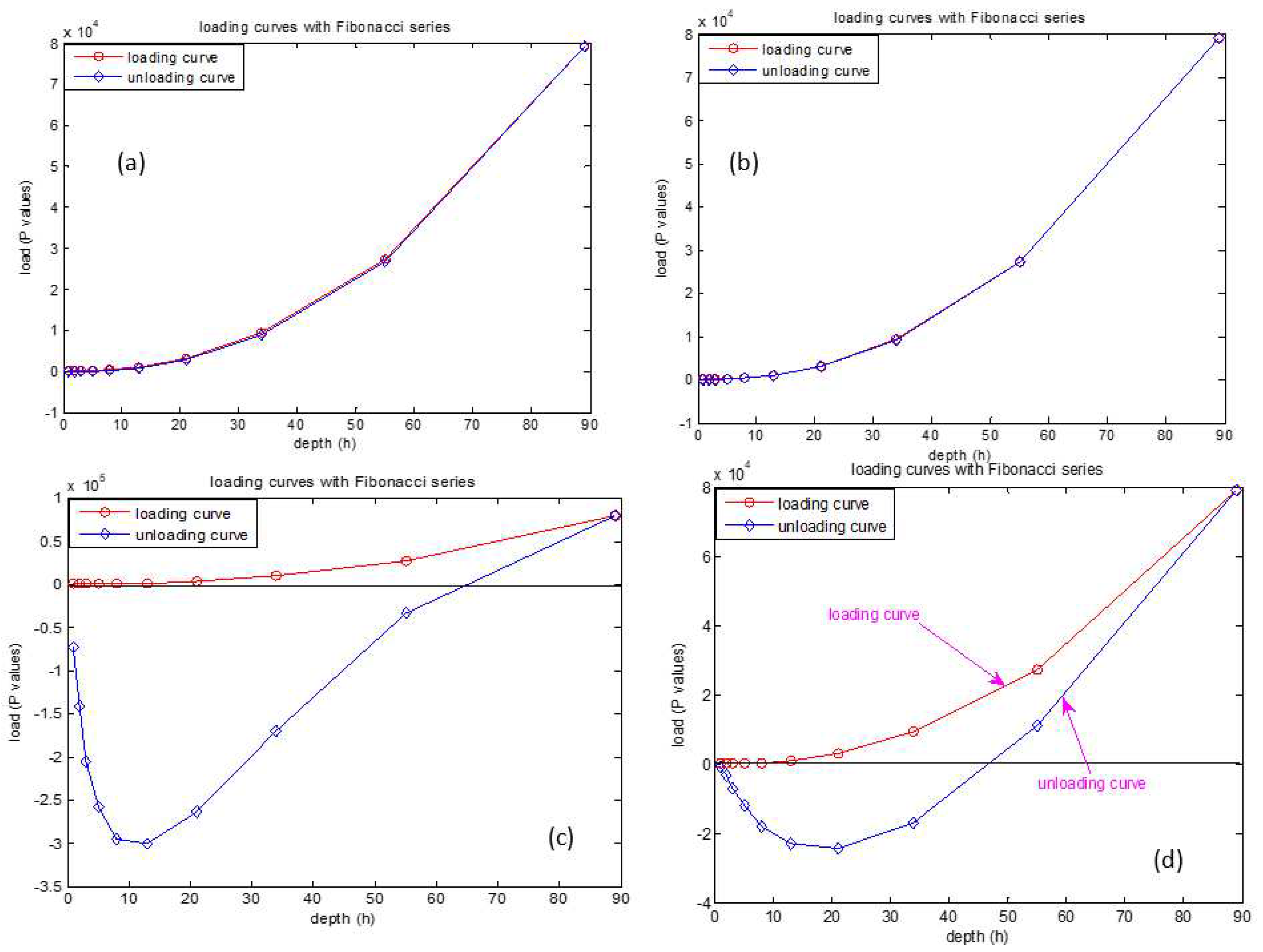
Figure 5)
By observing above curves, the third curve (i.e., P3) fails to have unloading curve structure. But according to Fibonacci series we can predict H value and its value will be 0.5 (i.e., H=0.5) and if this is the case, as H has single value then we should get a straight line if we try to fit curves but we were unable to get the expected curve with the existing equations but, with the proposed equation we obtain the curve how we expected. Let us analyze the situation graphically.
According to above considerations the existing equations can be written as follows by substituting H values into the equation. Here, in order to have a unloading curve structure we exclude max(h) as it is, instead of substituting h=0.5 as there will not be any maximum or minimum value for a single value. And it is as a support for our unloading curve description, as we mentioned that the second part (i.e., max(h)-h) (it is common term and important for any unloading curve) will serve as generating unloading data points for an unloading curve.
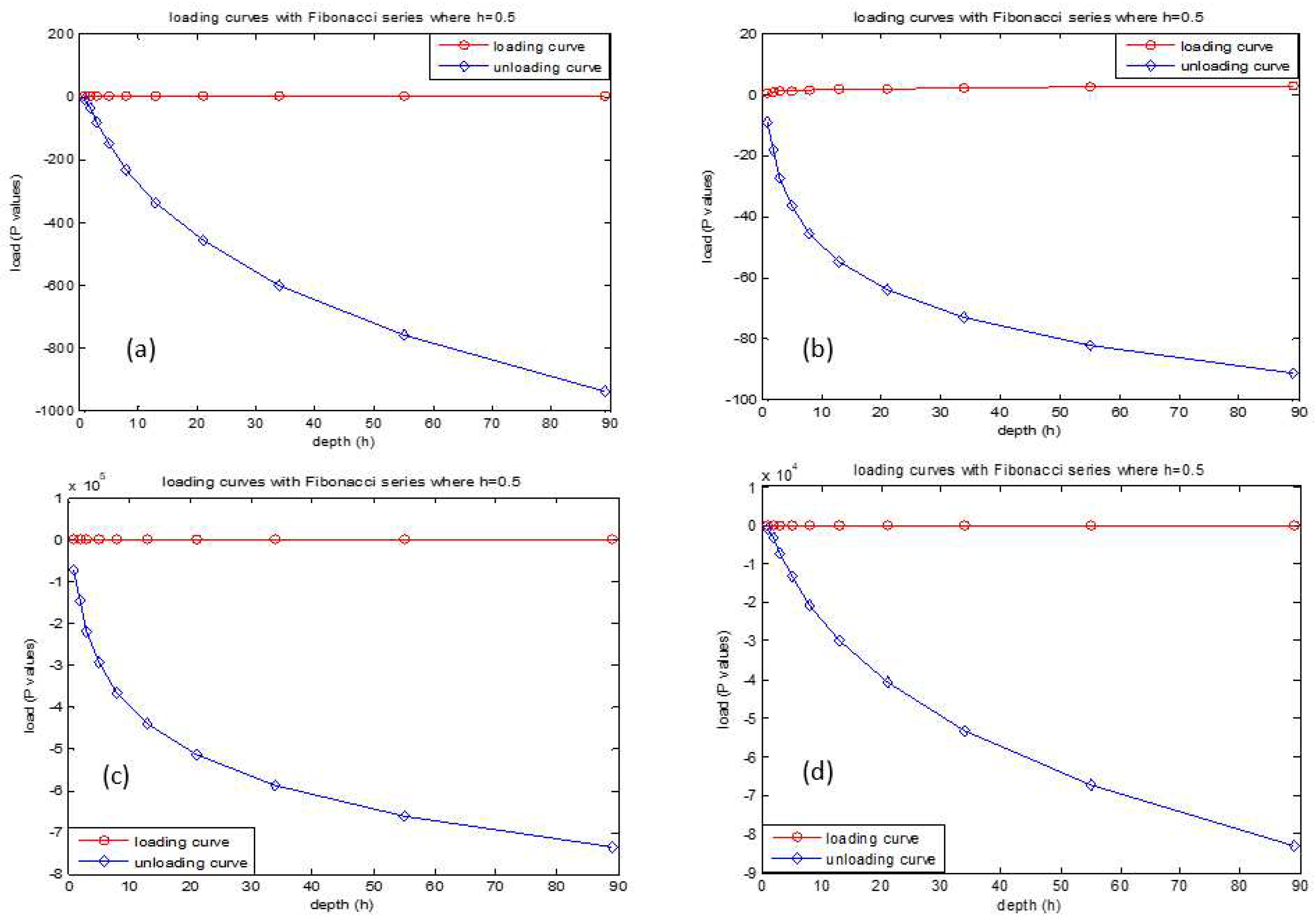
The loading part is common for all unloading equations so we eliminated mentioning each time for each curve; we mentioned only unloading curve equation for better understanding. The relevant curves are as follows (
Figure 6).
By observing all the graphically represented curves above, the curve fitting of loading and unloading is not up to the mark. The same considerations are made for the proposed equations and can be written as
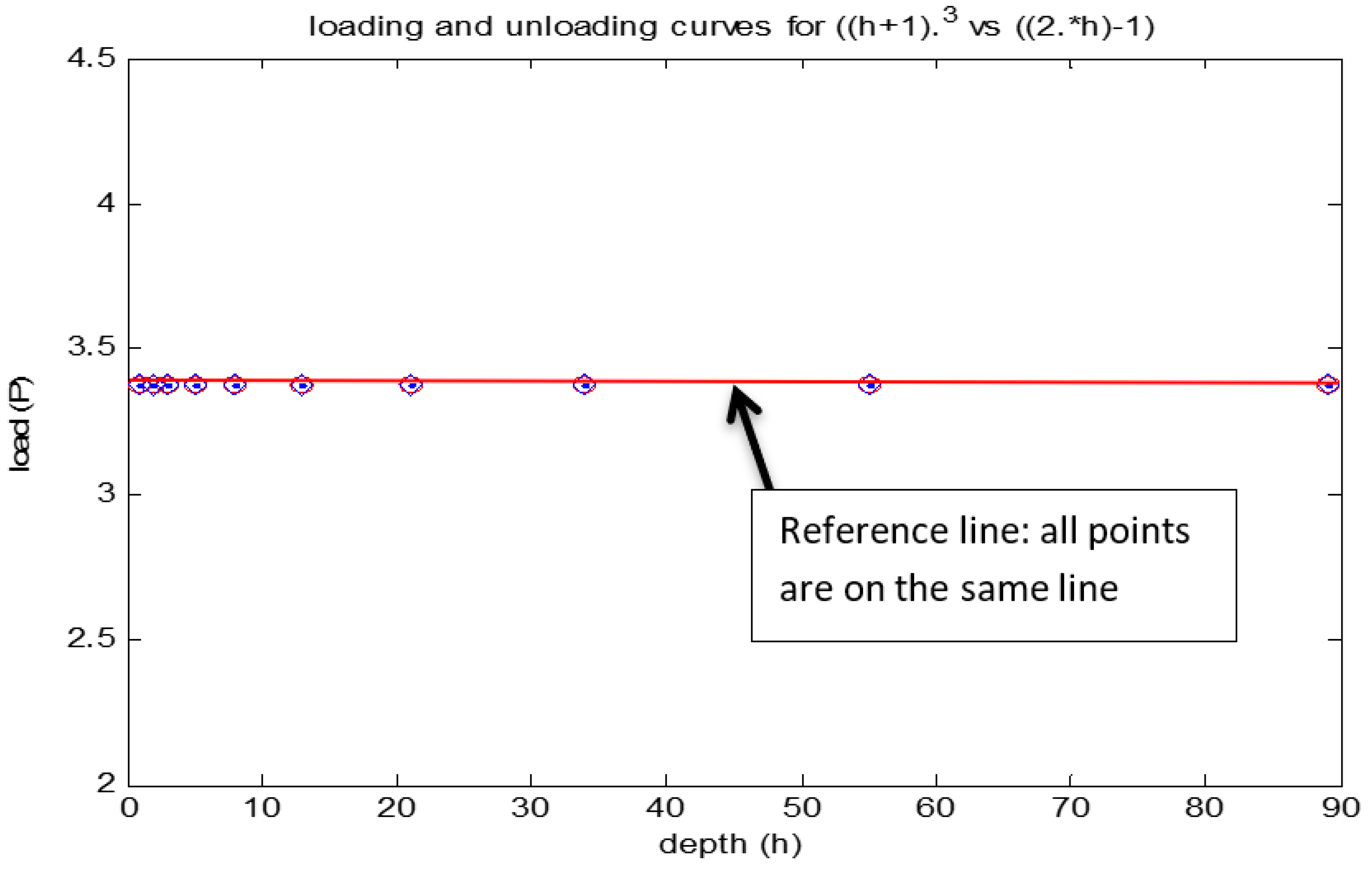
According to our assumption, we should get a straight line for loading and unloading curve equations for which the existing curve failed. The graphical representation of the curves as shown below. (
Figure 7)
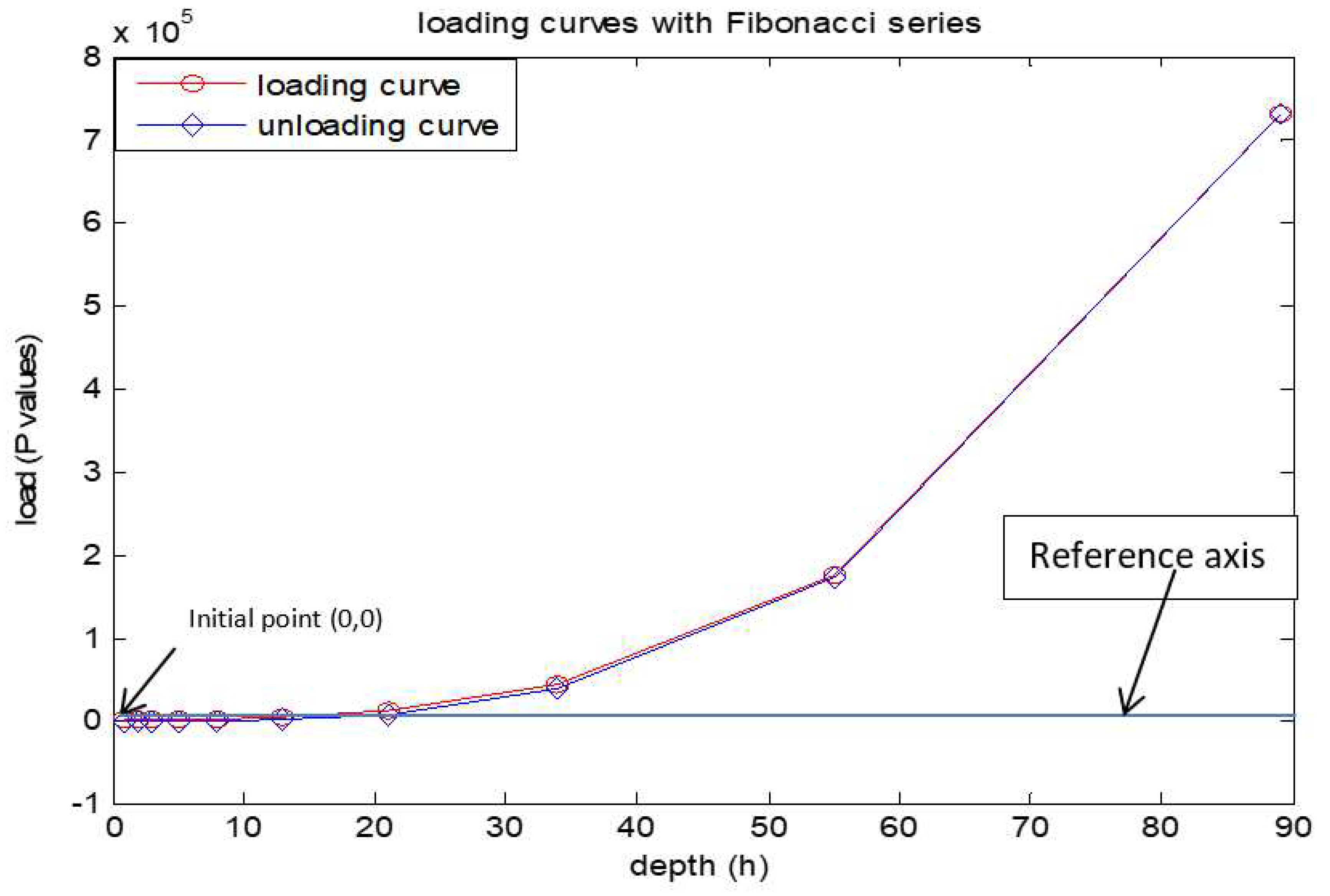
From the above graphical representation, the proposed equation satisfies the Fibonacci seriated data point too, and general curve fitting also done and represented below. The general equations are
By observing the above curve, we can assume that the curve indicates perfectly elastic body as it retrieved its original shape, as it reached its origin (
Figure 8). From above observations the proposed curves much perfect than the curves of existing. Therefor the proposed loading and unloading curve equations can be used for any type of data to fit.
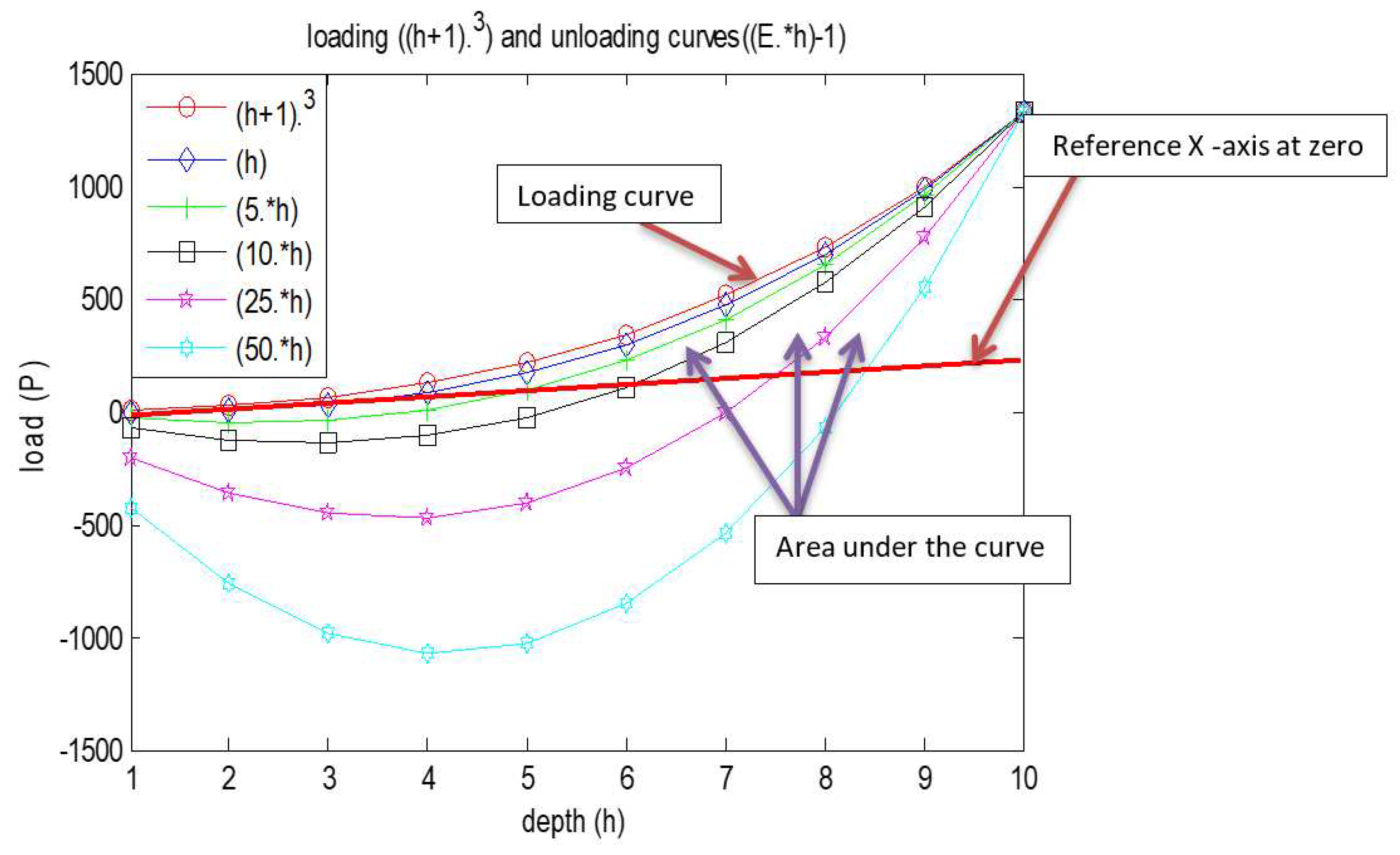
[C]. here, the area under the curve indicative of elasticity of a body, such a case the equations can be rewritten as
Here E indicates elasticity of the body, with the varying its values we obtain deferent are between the curves, and is such a case in the above equations and it is represented below graphically. For the instance E=[2 5 10 25 50] (
Figure 9) [
13]
3. Conclusion:
More generalized and easy equation for establishing relationship between loading and unloading curve was obtained, and elimination of unnecessary constants in the equation was achieved. The proposed equation fits with any type of data either seriated or no seriated data sets. New introduction of variable E was inserted, which specifies the area under the curve.
Supplementary
clc
clear all
h=1:10; %h=[1 2 3 5 8 13 21 34 55 89] (for Fibonacci series)
P=(h+1).^3;
P1=[(h+1).^3]-[(max(h)-h).*(2.*h)-1)];
plot(h,P,'ro-'); %loading curve
hold on
plot(h,P1,'bs-'); %unloading curve
hold off
legend('loading','unloading');
xlabel('depth (h)');
ylabel('load (P)');
title('loading and unloading curves');
With specific E values:
clc
clear all
h=1:10; %h=[1 2 3 5 8 13 21 34 55 89] (for Fibonacci series)
P=(h+1).^3;
P1=[(h+1).^3]-[(max(h)-h).*((2.*h)-1)];
P2=[(h+1).^3]-[(max(h)-h).*((5.*h)-1)];
P3=[(h+1).^3]-[(max(h)-h).*((10.*h)-1)];
P4=[(h+1).^3]-[(max(h)-h).*((25.*h)-1)];
P5=[(h+1).^3]-[(max(h)-h).*((50.*h)-1)];
plot(h,P,'ro-') %loading curve
hold on
plot(h,P1,'bd-'); %unloading curve
plot(h,P2,'g+-'); %unloading curve
plot(h,P3,'ks-'); %unloading curve
plot(h,P4,'mp-'); %unloading curve
plot(h,P5,'ch-'); %unloading curve
hold off
legend('(h+1).^3','(h)','(5.*h)','(10.*h)','(25.*h)','(50.*h)');
xlabel('depth (h)');
ylabel('load (P)');
title('loading ((h+1).^3) and unloading curves((E.*h)-1)');
With varying E values:
clc
clear all
h=1:10; %h=[1 2 3 5 8 13 21 34 55 89] (for Fibonacci series)
E=1:10;
P=(h+1).^3;
for i=1:10
for j=1:10
P1(i,j)=[(h(i)+1).^3]-[(max(h)-h(i)).*((E(j).*h(i))-1)];
end
end
plot(h,P,'ro-'); %loading curve
hold on
plot(h,P1,'bs-'); %unloading curve
hold off
legend('loading','unloading');
xlabel('depth (h)');
ylabel('load (P)');
title('loading and unloading curves');
References
- R. Dash, K. Bhattacharyya, A.S. Bhattacharyya, Film failure at earlier and later stages of nanoindentation in static and sliding mode. Eng Fail Anal (2023) 150, 107353. [CrossRef]
- R. Dash, K. Bhattacharyya, A. S. Bhattacharyya. Fracture associated with static and sliding indentation of multicomponent hard coatings on silicon substrates, Fatigue & Fracture of Engineering Materials & Structures (2023) 46: 1641-1645. [CrossRef]
- Ritambhara Dash, A. S. Bhattacharyya Crack growth based on indentation along substrate and nanocrystallites in Titanium diboride thin films, Fatigue & Fracture of Engineering Materials & Structures. (2023) 46 (7) 2714-2719. [CrossRef]
- R. Dash, R. P. Kumar, K. Bhattacharyya, A. S. Bhattacharyya, Intensified chipping during nanoindentation and the effect of friction on the interfacial fracture for thin films used in N/MEMS, IOP- Engineering Research Express, 2022 4 045012. [CrossRef]
- R. Dash, A. S. Bhattacharyya. Failure regions resembling geometrical shapes in sliding nanoindentation of Si-C-N thin films used for N/MEMS, Tech Phy Lett, 2022. [CrossRef]
- R. Dash, A.S. Bhattacharyya, Nanoindentation and stress analysis of Si-based N/MEMS, Materials Today: Proceedings, Volume 66, Part 7, 2022, Pages 3233-3237, ISSN 2214-7853. P: analysis of Si-based N/MEMS, Materials Today. [CrossRef]
- Monalisa Char, Amit K. Chakraborty, Arnab S. Bhattacharyya, Abhijit Kar. A Comparative Study on the Influence of SAC305 Lead-Free Solder Sandwiched by Sn on the Micromechanical and Electrical Properties of the Joints. Adv. Eng. Mater. 2021, 2100679. [CrossRef]
- R. Dash, K. Bhattacharyya, A S. Bhattacharyya, Synergistic fractural features observed in Ti-B-Si-C hard coatings on enhancing the sharpness of nano indenters, Int J. Ref Met & Hard Mater, 116, 2023 106373. [CrossRef]
- S. Bhattacharyya, R. Praveen Kumar, V. Ranjan, Gaurav Kumar, Nanoindentation and Scratch test of Thin Film Energy Materials, Current Smart Materials 2(1): 39 – 43, 2017. [CrossRef]
- A.S. Bhattacharyya, R. P Kumar, S. Priyadarshi, Sonu, S. Shivam, S. Anshu. Nanoindentation stress-strain for fracture analysis and computational modeling for hardness and modulus. J. Mat. Engg & Perform, 27, 2719–2726(2018) 20 March 201. [CrossRef]
- Oliver WC, Pharr GM. An improved technique for determining hardness and elastic modulus using load and displacement sensing indentation experiments. J Mater Res 1992; 7(6):1564–83. [CrossRef]
- AS Bhattacharyya, Computational studies of the nanoindentation load depth curves, J. Sc. & Ind. Res. 74 (4), 2015, 223-224.
- Kumar RP, Sanatnu Mitra, Bhattacharyya AS, Nanoindentation Fracture and Computational studies on hard coatings using initial value substitution algorithm, SciFed J Met Sci, 2017, 1:1.
|
Disclaimer/Publisher’s Note: The statements, opinions and data contained in all publications are solely those of the individual author(s) and contributor(s) and not of MDPI and/or the editor(s). MDPI and/or the editor(s) disclaim responsibility for any injury to people or property resulting from any ideas, methods, instructions or products referred to in the content. |
© 2024 by the authors. Licensee MDPI, Basel, Switzerland. This article is an open access article distributed under the terms and conditions of the Creative Commons Attribution (CC BY) license (http://creativecommons.org/licenses/by/4.0/).
