Research on the Evaluation and Influencing Factors of China's Provincial Employment Quality Based on Principal Tensor Analysis

This study aimed to use spatiotemporal tensor data to measure the level of employment quality in China's provinces and analyzed the magnitude and direction of its influencing factors in the spatiotemporal dimension. Taked 30 provinces, autonomous regions and municipalities directly under the central government in China from 2011 to 2020 as the research object, the employment quality evaluation system was constructed from six dimensions of employment environment, employment status, employability, labor remuneration, social security, and labor relations. The employment quality index data was expressed as a three-order high-dimensional tensor spatio-temporal data form, and the employment quality of China's provinces was measured from the spatio-temporal perspective by using principal tensor analysis, and the visual analysis of the development and change process of employment quality was carried out. The spatial autocorrelation analysis of employment quality was carried out, and the time-space dual fixed effect model of the spatial Dubin model was selected to analyze the direction and magnitude of the influence factors of employment quality on itself and its neighboring provinces. The research showed that: (1) The overall level of employment quality in China was not high and the employment quality varies greatly among provinces, and the employment quality development gap among provinces showed a trend of widening. (2) The development of employment quality in western China was relatively fast, while the development of employment quality in central China showed insufficient stamina. (3) Sichuan Province had a strong radiation effect on the development of employment quality in neighboring provinces, and Beijing and Tianjin had a strong siphon effect on the development of employment quality in neighboring provinces. (4) The level of industrialization and informatization promoted the development of employment quality in China's provinces, while the industrial structure had a significant negative effect on the development of employment quality.

Keywords:

Subject: Social Sciences - Decision Sciences

1. Introduction

The 20th National Congress of the Communist Party of China pointed out that employment was the basic livelihood of the people. Strengthening employment policy priorities, and improve the mechanism of employment, promote high quality full employment. China's 14th Five-Year Development Plan and 2035 long-term goals require that we improve the promotion mechanism that was conducive to more sufficient and higher-quality employment, expand employment capacity, improve employment quality, and alleviate structural employment contradictions. The Chinese government attaches great importance to people's livelihood and well-being, and strives to promote employment development in both quality and quantity. At present, China's economic growth rate has dropped from 10% to about 7%, and economic development is an important support for ensuring employment and people's livelihood. In the context of slowing economic growth, how to ensure the quality and quantity of employment? How to scientifically measure the quality of employment? What are the key factors in the development of employment quality? China is the largest developing country in the world, with the largest population and a large population density. China's national conditions have their own particularities and compatibility. Firstly, there are imbalances in China’s industrial development level, education distribution, industrial structure distribution, and digital innovation distribution; Secondly, there is a large difference in economic development between the east and west of China, and the supporting industries for economic development are different, resulting in significant differences in time and space. Therefore, it is more scientific to study China’s employment quality from a temporal and spatial perspective.

2. Literature review

2.1. Research on the measurement of employment quality

GROSSMANN V. summarized that the European Union's research on employment quality mainly focuses on two aspects: labor market and 6employment characteristics (GROSSMANN V, 2002). ARRANZ J. M et al. measured employment quality in three dimensions: working conditions, skills and training, and work-life balance (ARRANZ J. M., 2018). CHRENEKOVÁ M. et al. incorporated decent work into the employment quality evaluation system (CHRENEKOVÁ M. et al.,2016). Some scholars also use questionnaires to eliminate unreasonable indicators in the employment quality evaluation system (COCKS E., 2015, AERDEN K. V., 2016). Ming Juan et al. built an employment quality evaluation system with four dimensions, including income, working hours, labor contract and social security, and measured the employment quality of migrant workers through a multidimensional employment quality index (Ming J.,2015). Li Ning et al. analyzed the existing employment quality index system and gave statistical suggestions on employment quality (Li N.,2016). Zheng H. L. et al. constructed an employment quality evaluation system with five dimensions, including wage level, job conversion, labor contract, social security and subjective evaluation of immigrants, and calculated the employment quality index by simple average method (Zheng H. L.,2018). Mao J. J. et al. built an evaluation system in four dimensions: income, working hours, labor contracts, and social security, and measured the employment quality index by the equal-weighted average method (Mao J. J.,2020). Ling L. constructs an employment quality evaluation system in four dimensions: income level, working hours, social security, and employment satisfaction, and calculates the employment quality index through CRITIC empowerment (Ling L., 2022).

2.2. Research on Factors Affecting Employment Quality

Scholars use different methods to measure factors affecting employment quality from different angles. Chen G. S. et al. analyzed the impact of human capital investment on rural non-agricultural employment in Hunan Province based on time series data (Chen G. S., 2015). Yang Y. L. et al. used impulse response analysis to test the impact of urbanization level on employment quality in China (Yang Y. L., 2016). Zheng H. L. et al. measured the correlation between employment structure, industrial structure and economic growth (Zheng H. L., 2018). Ma R. studied the impact of government fiscal expenditure on labor employment by constructing a spatial Durbin model (Ma R., 2019). Sheng Yinan studied the impact of fertility policy adjustments on women's employment quality through the double difference method. Xie M. M., et al. analyzed the impact of artificial intelligence and technological progress on low-skilled employment in manufacturing (Xie M. M., 2019). Zhou C. used the endogenous transformation model to analyze the impact of government training on the employment of migrant workers (Zhou C., 2021). Zhang M. Z. et al. studied the impact of external tariff changes on regional labor employment in China (Zhang M. Z., 2022).

To sum up, although there are many studies on employment quality in the existing literature, there are two deficiencies. (1) In the research of employment quality evaluation, there is no scientific explanation for the construction of employment quality evaluation system. When measuring employment quality, the traditional principal component analysis method and entropy value method are mostly used. These methods can only measure employment quality in time dimension, and do not support the comprehensive measurement of employment quality in time and space dimension. (2) In the research on the factors affecting the quality of employment, it mainly analyzes how the factors affecting the quality of employment affect itself, ignoring the spatial correlation of the quality of employment, that is, ignoring the effects of the factors affecting the quality of employment in neighboring provinces on itself.

This paper's research focus is on the 30 provinces, autonomous regions, and municipalities (hereinafter referred to as provinces) in China excluding the Tibet Autonomous Region, Hong Kong, Macao, and Taiwan. We have collected employment quality-related index data from these 30 provinces in China from 2011 to 2020. We have organized and constructed a third-order high-dimensional data of the employment quality evaluation index system based on tensor structure. Principal Tensor Analysis 3 model was used to analyze the employment quality evaluation index system. Through the fiber operation and slice operation of the tensor, the dimensional reconstruction feature analysis and visual expression of the index system were carried out. Explore the spatial correlation of provincial employment quality and establish a spatial econometric model to analyze the magnitude and direction of the impact of each province's employment development on the economic and social development of its own and neighboring provinces, thereby providing data support and theoretical support for the government and enterprises to formulate policies.

3. Research methods

The purpose of this study was to use spatiotemporal data to measure China's provincial employment quality, further determine the spatial correlation of China's provincial employment quality, and determine the size and direction of the factors affecting employment quality. (1) PTA3 method was designed to decompose the comprehensive interaction of multi-dimensions and multi-features, and could reduce the dimensionality of high-order and high-dimensional data without changing its order. It overcomed the disadvantage of processing spatiotemporal multi-dimensional data in a sequential manner while ignoring its multi-linear structure. Therefore, this study applied the PTA3 method to measure employment quality from a spatio-temporal perspective for the first time, making up for the shortcomings of existing research that ignored the comprehensive role of multi-dimensional and multi-features in the employment quality evaluation system. (2) Global spatial autocorrelation was selected to analyze the spatial correlation of employment quality. (3) The spatial econometric model could analyze the direction and magnitude of the impact of factors affecting employment quality on itself and neighboring provinces from a spatial perspective.

3.1. PTAk Model of k-order Tensor (K>2)

PTAk represents a technique for decomposing complex, high-dimensional array data, known as N (N>2)-order tensors. This approach extends the well-known principal component analysis to higher dimensions. PTAk's core objective is to approximate intricate high-order tensors using simpler, low-order ones, facilitating feature extraction from intricate high-dimensional datasets. Essentially, it functions as a generalized singular value decomposition model. The method relies on the alternating least squares technique to compute the principal tensor efficiently. This process enables the extraction of orthogonal sub-tensors from the original data, providing an effective approximation of the high-dimensional space. The significance of the principal tensor is evaluated based on the magnitude of its singular value, ensuring reliability in its selection.

Historically, the processing of spatiotemporal multidimensional data has often involved converting it into a sequential vector format for analysis within a linear subspace. However, this approach neglects the inherent multilinearity of such data. Analogous to the limitations of a two-way analysis table that can only be collapsed or expanded in two dimensions, traditional methods often overlook the rich interactions present in higher-order data. PTAk's framework addresses this by incorporating duality principles, thereby broadening the scope of multidimensional analysis to better capture the complexities of spatiotemporal datasets. The structural form of PTAk for tensors of order k is described as follows:

The first principal quantity, the optimized form of singular value is as follows:

σ_{1} = m a x X .. (ψ \otimes φ \otimes ϕ)

(1)

{| | ψ | |}_{s} = 1

{| | φ | |}_{v} = 1

{| | ϕ | |}_{t} = 1

= X (ψ_{1} \otimes φ_{1} \otimes ϕ_{1})

In this context, "⊗" signifies the tensor product, while ".." indicates the contraction operation, which is akin to the inner product operation in the tensor space. The letter "X" serves as a placeholder for matrix or tensor data from the same dataset. The symbols

ψ_{1}, φ_{1}, ϕ_{1}

represent the first principal components. When combined,

ψ_{1} \otimes φ_{1} \otimes ϕ_{1}

is designated as the primary component. This approach allows us to determine the most precise rank-one approximation, along with the singular value, for a given tensor X. The specific calculation technique used in this step is known as the RPVSCC algorithm. This algorithm is equivalent to TUCKALS3, which focuses on selecting only one component per module. The uniqueness of the tensor solution given by Eq. (1) under orthogonal transformation was first established by Leibovici in 1999 (Leibovici D., 1999).

The PTAk model offers a more convenient calculation method because, instead of directly employing algebraic methods to calculate the tensor product of vectors, it employs the contraction operator, as described in Eq.(2). This approach streamlines the computational process and makes it more efficient.

X .. (ψ \otimes φ \otimes ϕ) = (X .. ψ) .. (φ \otimes ϕ)

(2)

= (X .. φ) .. (ψ \otimes ϕ)

= (X .. φ) .. (ψ \otimes φ)

= ((X .. ψ) .. φ) .. ϕ

To solve for the second principal tensor, an orthogonality constraint is introduced to Eq.(1). This optimization process mirrors the preceding step in the solution methodology, focusing on the projection of tensor X onto the orthogonal tensor of the initial argument, denoted as

P_{(ψ_{1}^{⊥} \otimes φ_{1}^{⊥} \otimes ϕ_{1}^{⊥})} X

. Notably,

ψ_{1}^{⊥} \otimes φ_{1}^{⊥} \otimes ϕ_{1}^{⊥}

represents the orthogonal tensor of the first principal tensor and can alternatively be expressed as

(I d - P_{ψ_{1}}) \otimes (I d - P_{φ_{1}}) \otimes (I d - P_{ϕ_{1}})

According to Eq.(3), the PTAk decomposition offers a method for synthesizing data from a set of uncorrelated components. In the schemas utilized for PTA3(X) and PTAk(X), it's possible to distinguish between the principal tensor and its associated principal tensor. The associated tensors are connected to the principal tensor because they display one or more of its components within the first principal tensor's component set. After a tensor of rank k performs a contraction operation on a given component, the associated principal tensor quantity can be decomposed using PTA(k-1). This makes the PTAk algorithm a recursive algorithm. When k=3, there are specific instances where this decomposition applies.

PTA 3 (X) = σ_{1} (ψ_{1} \otimes φ_{1} \otimes ϕ_{1}) + ψ_{1} \otimes_{1} P T A 2 (P (φ_{1}^{⊥} \otimes ϕ_{1}^{⊥}) (X .. ψ_{1}^{⊥})) + φ_{1} \otimes_{2} P T A 2 (P (ψ_{1}^{⊥} \otimes ϕ_{1}^{⊥}) (X .. φ_{1}^{⊥})) + ϕ_{1} \otimes_{3} P T A 2 (P (ψ_{1}^{⊥} \otimes φ_{1}^{⊥}) (X .. ϕ_{1}^{⊥})) + P T A 3 (P (ψ_{1}^{⊥} \otimes φ_{1}^{⊥} \otimes ϕ_{1}^{⊥}) X)

(3)

The notation

\otimes_{1}

means that in this full tensor product operation, the vector on the left will occupy the ith position in k positions, such as

φ_{1} \otimes_{2} (α \otimes β) = α \otimes φ_{1} \otimes β

PTA3 Model Algorithm

Before introducing the algorithm of the PTAk model, a brief overview of the RPVSCC algorithm is provided. The objective of the RPVSCC algorithm is to identify the principal tensor quantity of the initial tensor X. Detailed pseudocode for this algorithm will be provided later.

RPVSCC algorithm(k=3)

Input: Tensor X, maximum iteration step size MAX and stop iteration threshold ɛ

Output: singular value σ and its principal tensor components α, β, γ

step:

1: Initialize a set of principal tensor components

α_{0}

β_{0}

γ_{0}

2: for i from 1 to MAX:

(X .. β_{i - 1}) .. γ_{i - 1} = σ_{i}^{α} α_{i}

(X .. γ_{i - 1}) .. α_{i} = σ_{i}^{β} β_{i}

(X .. α_{i}) .. β_{i_{i}} = σ_{i}^{γ} γ_{i}

If the extreme value of

σ_{i}^{α}

σ_{i}^{β}

σ_{i}^{γ}

is less than ɛ, jump out of the iteration loop and output

σ_{i}

α_{i}

β_{i}

γ_{i}

。

The pseudocode of the complete PTAk algorithm is as follows:

PTAk algorithm(k=3)

Input: tensor X, order k=3, maximum iteration step size MAX and stop iteration threshold ɛ

Output: principal tensor

A_{i}

,i=1,2,

\dots

,m, associated principal tensor

A_{i}^{j}

,j=1,2,

\dots

step:

1: Run the RPVSCC algorithm to get the principal tensor

A_{i} = S_{i}^{1} \otimes S_{i}^{2} \otimes \dots \otimes S_{i}^{k}

2: On the orthogonal tensor space of the solution obtained in step 1, repeat step 1 to obtain all principal tensors.

3: for i from 1 to m:

For j from 1 to k:

X_{i}^{j} = X .. S_{i}^{j}

A_{i}^{j} = P T A (k - 1) * X_{i}^{j}

return

A_{i}^{j}

In the PTAk algorithm's pseudocode, for a given i, j,

A_{i}^{j}

may not always represent only the associated principal tensor quantity. This is because the

P T A (k - 1) * X_{i}^{j}

optimization can select multiple associated principal tensors. Additionally, the singular value of each principal tensor quantity obtained may not be larger than the singular value of all associated principal tensors. This is because the singular value of the associated principal tensor of the ith principal tensor may be larger than that of the i+1th principal tensor.

3.2. Global spatial Autocorrelation analysis

Global spatial autocorrelation analysis is to analyze whether a phenomenon exists spatial correlation in the study area, that is, to describe the spatial distribution of carbon emissions in our country from the perspective of space. Moran's I is a commonly used index, and the formula of Moran's I is as follows:

I = \frac{\sum_{i = 1}^{n} \sum_{j = 1}^{n} W_{i j} (X_{i} - \bar{X}) (X_{j} - \bar{X})}{S^{2} \sum_{i = 1}^{n} \sum_{j = 1}^{n} W_{i j}}

(1)

In Formula (1),

W_{i j}

is any element of the binary space weight matrix,

X_{i}

and

X_{j}

is the carbon emission score value of the

i

and

j

regions,

n

is the total number of regions, and

S^{2}

is the sample variance. In this study, the definition

W_{i j}

is as follows:

W_{i j} = {\begin{matrix} 1, W h e n r e g i o n i i s a d j a c e n t t o r e g i o n j \\ 0, W h e n r e g i o n i i s n o t a d j a c e n t t o r e g i o n j \end{matrix}

(2)

The value range of Moran's I is -1≤Moran's I≤1. If Moran's I is positive, it indicates that the carbon emission of each province presents a positive spatial correlation. If Moran's I is negative, it means that the carbon emission of each province presents a spatial negative correlation. If Moran's I is zero, it means that the carbon emissions of each province are irrelevant. Moran's scatter plot can divide our provincial carbon emissions into four spatial dependence patterns, which are located in four quadrants. In the first quadrant, provinces with high carbon emissions are surrounded by provinces with also high carbon emissions (HH), in the second quadrant, provinces with high carbon emissions are surrounded by provinces with low carbon emissions (HL), in the third quadrant, provinces with low carbon emissions are surrounded by provinces with high carbon emissions (LH), and in the fourth quadrant, provinces with low carbon emissions are surrounded by provinces with also low carbon emissions (LL).

For the calculation results of Moran's I index, two hypotheses of asymptotic normal distribution and random distribution can be used respectively to test the standardized formula as follows:

Z (d) = \frac{M o r a n' s I - E (M o r a n' s I)}{\sqrt{V A R (M o r a n' s I)}}

(3)

The expected value formula of standardized Moran's I can be calculated according to the distribution of geospatial data as follows:

E (M o r a n ’ s I) = \frac{1}{n - 1}

(4)

3.3. Spatial metering model

According to the "first law of geography", all things are interrelated with other things, and things near are more relevant than things far away. Spatial metrology is to study the correlation between things. Currently, the commonly used spatial metrology models include spatial lag model (SLM), spatial error model (SEM), and spatial Dubin model (SDM). In this study, a spatial econometric model was established to analyze the influencing factors of China's inter-provincial carbon emissions.

(1) Spatial lag Model (SLM)

The spillover effect of carbon emissions from neighboring provinces to their own province is mainly analyzed, that is, the size and direction of the spatial influence of carbon emissions from neighboring provinces on carbon emissions of a certain province. The model is as follows:

Y_{i t} = δ \sum_{j = 1}^{n} W_{i j} \times Y_{j t} + \sum_{k = 1}^{m} β_{k} X_{i k t} + μ_{i} + λ_{i} + ε_{i t}

(5)

In formula:

Y_{i t}

is the explained variable;

i

j

is the province;

n

is the number of provinces;

t

is the year;

W

is the space weight matrix;

δ

is the spatial autoregressive coefficient;

X

is the explanatory variable;

β_{k}

is the coefficient of the

k

explanatory variable;

m

is the number of explanatory variables;

μ_{i}

is the spatial fixed effect;

λ_{i}

is time fixed effect;

ε_{i t}

is random error.

(2) Spatial Error model (SEM)

This paper mainly analyzes the differences of carbon emissions among provinces affected by geographical location, and represents the impact of carbon emission error impact of neighboring provinces on regional carbon emissions. The model is as follows:

Y_{i t} = \sum_{k = 1}^{m} β_{k} X_{i k t} + μ_{i} + λ_{i} + ϕ_{i t}

(6)

ϕ_{i t} = ρ \sum_{j = 1}^{n} W_{i j} \times φ_{i t} + ε_{i t}

(7)

In formula:

φ_{i t}

is the spatial autoregressive error term;

ρ

is the spatial autocorrelation coefficient of the error term.

(3)Spatial Durbin Model (SDM)

This paper mainly analyzes the influence of influencing factors of carbon emissions in the province on carbon emissions in the local and neighboring provinces, and can investigate the influence of spatial lag term on carbon emissions. The model is as follows:

Y_{i t} = δ \sum_{j = 1}^{n} W_{i j} \times Y_{j t} + \sum_{k = 1}^{m} β_{k} X_{i k t} + θ \sum_{k = 1}^{m} W_{i j} \times X_{j k t} + μ_{i} + λ_{i} + ε_{i t}

(8)

In formula:

θ

is the coefficient of spatial lag explanatory variable.

4. China’s inter-provincial employment quality measurement and visualization

First, the paper constructed the Chinese provincial employment quality evaluation system; Then the paper used PTA3 model to reduce dimension, extracted principal components, analyzed the quantitative comprehensive evaluation index of key elements, and calculated the comprehensive score of employment quality in each province. Finally, the paper expressed the employment quality visually according to the scores of each province (Gao X. D., 2022).

4.1. Measurement of provincial employment quality in China

(1) Construction of China’s inter-provincial employment quality evaluation index system

The construction of employment quality evaluation system needed to take into account multiple evaluation positions and perspectives of society, workers and government. The employment environment and conditions provided by the economic and social development were the basis of the employment of the workers, the ability of the workers and the labor remuneration were the inevitable guarantee of employment, and the social security and labor relations protection provided by the government were the guarantee of the employment of the workers. Therefore, we measured employment quality from six dimensions: employment environment, employment status, employability, labor remuneration, social security, and labor relations, and analyzed the data from 30 provinces in China from 2011 to 2020. The construction of the three-level indicators of the employment quality indicator system referd to the author’s previous research. The evaluation results of employment quality were shown in Table 1.

(2) Data preprocessing

The original data of the employment quality evaluation system indicators come from the 2011-2020 "China Statistical Yearbook", "China Population and Employment Statistical Yearbook", "China Labor Statistics Yearbook" and provincial statistical yearbooks. For some missing data, the mean interpolation was used, and the outliers in the statistical yearbook were adjusted on the basis of analyzing the development trend. When constructing spatio-temporal tensor data, space was denoted as module 1, time as module 2, and index as module 3. The research focused on the spatio-temporal dynamics of the index, that is, the variable of interest was module 3, and the other two modules were its support, so the relationship between modules 1,2 and the related variables of module 3 should be looked for. Mode 3 data were double centralized and normalized along mode 1 and mode 2 to emphasize the interaction between spatiotemporal trends and mode 3. Based on the tensor structure, the pre-processed data was organized into multidimensional spatiotemporal data by using R statistical software to form tensor data that could be arbitrarily decomposed and combined in time and space. After organizing, the dimensions of the tensor were (30,10,18).

(3) Calculation results of PTA3

Using the PTA3 model, we conducted principal tensor analysis on organized tensor data to obtain the principal tensor component coefficients for each tensor and dimension. Table 2 highlights the principal tensors with variance contribution rates exceeding 0.01%. The four largest singular values are 53.7118, 23.4939, 18.9946, and 8.8380, corresponding to the first principal tensor (vs111), the sixth principal tensor, the seventh principal tensor, and the second principal tensor (vs222), respectively. The variance contribution rates of these principal tensors to the overall data are 53.60%, 10.25%, 6.70%, and 1.45%, respectively, with a cumulative contribution rate of 72%.

(4) Employment quality principal tensor coefficient

The scoring coefficients of the four principal tensors in any dimension were calculated based on the first four largest singular values of the initial tensor and their corresponding principal tensors. Table 3 displays the score coefficients of these four principal tensors in the index dimension. The four tensors could be expressed as:

U_{i} = X F_{i}, i = 1, 2, 3, 4;

(

X = (X_{1}, X_{2}, \dots, X_{18}))

. The weights of each principal tensor were:

ω_{1} = \frac{53.6}{72} = 0.7444, ω_{1} = \frac{10.25}{72} = 0.1424, ω_{1} = \frac{6.7}{72} = 0.0931, ω_{1} = \frac{1.45}{72} = 0.0201

. The comprehensive index of employment quality score was Y, then Y could be expressed as:

Y = \sum_{i = 1}^{4} ω_{i} U_{i}

The same method can be used to obtain the score coefficients of each principal tensor in the time dimension. The scoring coefficients of the first and second principal tensors on modules 1 and 2 are shown in Figure 1. In general, when measuring the status of employment quality in space, the more recent years have greater weight, as shown in Figure 1. Therefore, the score coefficient is reasonable.

4.2. Visualization of employment quality in China's provinces

Since tensor decomposition is holistic and supports reconstruction features, the spatio-temporal data organized based on tensor structure can be expanded in all dimensions, and different dimensional components can be recombined. For the concerned index dimension, its performance in time dimension, space dimension or space-time synthesis dimension can be obtained. The results of the PTA3 model have included the scoring coefficients obtained by expanding each principal tensor in the direction of modules 1, 2 and 3 respectively. Their tensor product can approximate the original spatio-temporal data, and the perspective information in any two dimensions can be reconstructed by the tensor product of the score coefficients of these two dimensions, so as to achieve the coupling feature extraction of the original spatio-temporal data in different dimensions, and then reveal the development status of China's provincial employment quality from different perspectives. Based on the tensor-based fiber operation and slice operation, the score coefficient of the claim in different dimensions was used to calculate the comprehensive score of employment quality in each combination dimension and display it visually.

4.2.1. Expansion and visualization in spatial dimension

Based on the tensor's fiber operation, fixing the time dimension and index dimension, we obtained 10×18 tensor fibers along the spatial dimension. Four of these fibers were selected for visualization, and to more comprehensively exhibit the development of employment quality, the index dimension was fixed on the comprehensive employment quality score index calculated using the score coefficient Y. In the time dimension, the fibers were fixed at 2011, 2014, 2017, and 2020, respectively. Figure 2 displays these four sample fibers. After ranking based on the comprehensive employment quality score, the scores of the top regions exhibit significant differences, while the scores of the middle and lower regions are more concentrated. Therefore, the legend in Figure 2 does not employ a uniform partitioning approach. As shown in the figure, with the implementation of China's western development policy, the quality of employment in the western region has steadily improved; however, the central region exhibits insufficient development potential and is gradually being overtaken by the western region. The development span of the quality of employment in various provinces showed a trend of increasing and increasing, and the development of the quality of employment showed a significant unbalanced trend, which needed to be improved.

4.2.2. Expansion and visualization in time and space dimensions

Using the tensor slicing operation and the predefined index dimension, we obtained 18 slices of the tensor along the spatial and temporal dimensions. To present a comprehensive overview of employment quality development, these slices were fixed on the composite employment quality index Y for visual representation. The overall trend of the employment quality situation over time and region could be seen from Figure 3. From the perspective of the whole country, the average employment quality of China from 2011 to 2020 fluctuated around 1.3795, the overall level of employment quality was not high, but t it was showing an overall linear upward trend, indicating that our employment quality was developing healthily and improving steadily. From a provincial perspective, Beijing, Shanghai, and Tianjin rank highest in employment quality, followed by Zhejiang, Guangdong, and Jiangsu. Conversely, Jiangxi, Heilongjiang, and Henan rank lowest. In the past 10 years, the employment quality scores of Beijing and Shanghai have grown rapidly, firmly securing the top two spots and exhibiting increasingly evident advantages. Tianjin's employment quality score ranks third, but the gap between it and the top two is gradually widening, while the gap between it and the following provinces is narrowing.

From 2011 to 2020, Guizhou, Sichuan, Yunnan, Guangxi and Gansu provinces had a rapid increase in employment quality. These five provinces were all from the western region of China, indicating that the strategy of large-scale development of the western region was effective and the employment quality in the western region was steadily improving. The employment quality in Inner Mongolia, Anhui, Liaoning, Shanxi, Hebei, and Henan has rapidly declined. These six provinces are all located in the central and eastern regions. Although the quality of employment in these provinces has been steadily increasing, the increase has been small and the growth has been relatively slow.

It is worth noting that Sichuan Province has a strong radiation effect on the development of employment quality in neighboring provinces. It had become the core of driving the growth of surrounding employment quality between 2011 and 2020. As can be seen from Figure 4, Sichuan's neighboring provinces have all developed rapidly in employment quality driven by Sichuan. After Sichuan Province completed the post-disaster reconstruction work of the Wenchuan Earthquake in 2011, its economy has developed rapidly and has become the province with the fastest economic growth in recent years. While Sichuan is comprehensively developing its own employment quality, it has also had a strong radiation effect on neighboring provinces, driving the rapid development of employment quality in neighboring provinces Guizhou, Yunnan, Guangxi, and Gansu. Beijing and Tianjin had a strong siphon effect on the development of employment quality in neighboring provinces. The employment quality of the provinces near Beijing and Tianjin showed a downward trend.

5. Spatial econometric analysis of influencing factors of employment quality in China's provinces

5.1. Spatial correlation analysis of employment quality in China's provinces

Through exploratory spatial data analysis, the spatial correlation of China's inter-provincial employment quality is studied. As can be seen from Table 4, the global Moran I index of employment quality scores of 30 provinces in China from 2011 to 2020 is all greater than zero, and the statistical test value is all less than 0.05, indicating that China's inter-provincial employment quality presents significant spatial autocorrelation during the study period. Provinces with higher employment quality tend to be adjacent to provinces with higher employment quality in space, while provinces with lower employment quality tend to be adjacent to provinces with lower employment quality in space. Therefore, it is suitable for the spatial econometric analysis of the factors affecting the employment quality in China's provinces.

5.2. Analysis of influencing factors of employment quality in China's provinces

Through spatial autocorrelation analysis, it can be found that China's inter-provincial employment quality has spatial correlation. Therefore, a spatial econometric model can be built to explore the impact of various influencing factors on China's inter-provincial employment quality.

5.2.1. Selection of variables and data test

According to the principles of representativeness and availability, relevant explanatory variables were selected based on the existing research and the actual situation of each region. The explained variables are employment quality score, and the explanatory variables are industrial structure, urbanization level, industrialization level, investment policy, foreign trade dependence, informatization level, price level, fiscal expenditure and technology level. As the fundamental purpose of the analysis of employment quality is to improve the employment imbalance, economic development has a stronger and more significant impact on employment quality, so more emphasis is placed on the consideration of variables related to economic factors, as shown in Table 5.

ADF-Fisher test method was used to conduct unit sum test on the variables used in the study. The stationarity test results showed that variables EQ, IS, IP, DFT, IT, FIS and TFP were zero-order unstable, and all variables showed stationarity results at the first and second order levels, indicating that the test variables had first-order stationarity. The results obtained from this set of data have scientific significance. In order to avoid the interference of heteroscedasticity on the empirical results, the regression analysis was carried out on the logarithm of the original data.

5.2.2. Regression results of spatial Durbin model

The Lagrange multiplier test (LM test) and its Robust test results show that the LM test corresponding to SLM and the Robust test both pass the 1% significance level test, and the LM test corresponding to the spatial error panel model SEM passes the 1% significance level test. The Robust test corresponding to SEM passes 1% significance level test, indicating that SLM is superior to SEM, and the test results of SLM and SEM are both significant, so it is necessary to further select SDM model for estimation and comparison. SDM regression results show (Table 4) that the R² of four SDM effects was 0.8968, 0.9761, 0.9098, 0.9862, respectively, with Log-likelihood being 112.0350, 323.6626, 127.5496, 401.9792, respectively. Error term squared (sigma2) and Log-likelihood value indicate that spatial fixed effects and spatial-time double fixed effects are better estimated. From the significance level of the regression results of SDM, the spatial-time double fixed effect is more significant than the estimation result of spatial fixed effect. Therefore, this study selects the spatial-time double fixed effect in SDM to analyze the influencing factors of employment quality. Wald and likelihood ratio test (LR test) of SDM under spatial-temporal dual fixed effects show that: The Wald test and LR test values of SLM are 93.8198 and 37.9455, and their adjoint probability values are 3.33E-16 and 1.78E-05, respectively. The Wald test and LR test values of SEM are 26.8987 and 1.9489, respectively. The adjoint probability values are 2.75E-14 and 2.00E-03 respectively, both of which pass the test at the significance level of 1%, indicating that the model does not degenerate into SLM and SEM.

5.2.3. Decomposition of spatial effects of factors affecting employment quality in China's provinces

The spatial-temporal dual fixed effect of SDM is selected to conduct a spatial econometric analysis on the quality of inter-provincial employment in China and its influencing factors from 2011 to 2020 (Table 6). In the table, the estimated coefficients of W*URBAN, W*IL, W*DFT and W*IT are all positive, and all are significant at the 1% level, which indicates that the spatial spillover effects of urbanization level, industrialization level, foreign trade dependence and informatization level on the surrounding provinces are positive. The estimated coefficients of W*IS, W*IP and W*Fical in the table are negative and all are significant at 1%, which indicates that the spatial spillover effects of industrial structure, investment policy and fiscal expenditure on the surrounding provinces are negative. Due to the spatial lag term, the estimated results of SDM cannot represent the marginal effects of the influencing factors, and the interpretation of the regression coefficient on the employment quality is not scientific. Further analysis of the direct effects, indirect effects and total effects of the influencing factors is needed.

The direct effect represents the influence of various factors affecting employment quality on the employment quality of the province. From the direct effect, it can be seen that the industrial structure, urbanization level, industrialization level, investment policy, foreign trade dependence, informatization level and technology level of each province have different degrees of influence on the employment quality of each province in China, and the significance level and effect strength of each variable are also different(Table 7). ➀ Industrialization level, investment policy and informatization level have promoting effects on employment quality, and industrialization level has the largest effect coefficient (0.1001) on urban development quality, followed by investment policy and informatization level. ➁ The effect of price level and fiscal expenditure on employment quality is not significant. ➂It is worth noting that urbanization level and industrial structure have a significant negative effect on the quality of inter-provincial employment in China.

The indirect effect represents the influence of factors affecting the employment quality of neighboring provinces on the employment quality of the province. From the indirect effect, we can see that the industrial structure, industrialization level and informatization level are significant at the level of 1%, the urbanization level and fiscal expenditure are significant at the level of 5%, and the investment policy and technology level are significant at the level of 10%, that is, the spatial spillover effect is significant. ➀ The influence of industrial structure, investment policy, fiscal expenditure and technical level on the employment quality of neighboring provinces is negative, and the change of investment policy will have a "siphon effect" on various labor resources in neighboring provinces. ➁ The influence of foreign trade dependence and price level on the employment quality of neighboring provinces is not obvious, that is, the development of these aspects has no effective radiation on the employment quality of neighboring provinces. ➂ It is worth noting that, like the direct effect, the industrial structure is a negative effect of spatial spillover.

The total effect is the comprehensive influence strength of the factors affecting the employment quality of each province on the employment quality of China's provinces. From the total effect, it can be seen that the industrial structure, urbanization level, industrialization level and informatization level pass the significance test of 1%, the technical level passes the significance test of 5%, and the investment policy, foreign trade dependence and fiscal expenditure pass the significance test of 10%. ➀ The effect coefficient of industrialization level and informatization level is positive, indicating that through industrialization development and informatization level improvement, China's employment quality will be improved accordingly. ➁ The total effect of industrial structure and urbanization level is negative, indicating that industrial structure and urbanization level have no promoting effect on employment quality.

Comprehensive analysis shows that the industrial structure has a significant negative effect on employment quality under the three effect models. In 2011, employment in the primary industry accounted for 34.74 percent and that in the tertiary industry 35.68 percent. In 2020, employment in the primary industry accounted for 23.60 percent and that in the tertiary industry accounted for 47.70 percent. At present, the number of employment in China's primary industry has decreased significantly, while the number of employment in the tertiary industry has grown rapidly. In the process of the development and change of industrial structure, the labor force of the primary industry is easily replaced by science and technology, so as to flow to the second and third industries. The traditional service industry absorbs a large number of labor transferred from the primary industry, resulting in the tertiary industry can not develop in high quality. At the same time, the reform of household registration system and land policy promoted the transfer of labor force in the primary industry, but due to the constraints of their own skills and industry thresholds, there are still large mobility barriers for the transfer of labor force in the primary industry between industries. Moreover, a large part of the transferred agricultural labor force flows into the traditional service industry, thus forming the "anti-efficiency allocation" of labor force factors. Hindering the healthy development of economic growth and employment quality.

6. Conclusion

(1) The overall level of employment quality in China is not high and the difference of employment quality between provinces is large, and the development gap of employment quality between provinces shows a trend of widening. Beijing, Shanghai and Tianjin ranked the top three in the overall score of employment quality, but the gap between Tianjin and Beijing and Shanghai was increasing, and the gap between Tianjin and the fourth place was gradually narrowing. Over the 10-year period, the provinces with the fastest growth in the overall score of employment quality are all from China's western regions, while the provinces with the fastest lag are from central and eastern regions.

(2) The development rate of employment quality in western China is fast, while the development of employment quality in central China is weak. As China's first-tier cities, Beijing and Shanghai exhibit strong development momentum, with the fastest growth rate of employment quality among the 30 provinces. Their advantages are becoming increasingly evident. However, with the implementation of China's western development policy, the quality of employment in the western region is steadily improving, while the central region exhibits insufficient development potential and is gradually being overtaken by the western region.

(3) Sichuan has a strong radiation effect on the employment quality development of neighboring provinces, while Beijing and Tianjin have a strong siphon effect on the employment quality development of neighboring provinces. While the employment quality of Sichuan develops rapidly, the employment quality of its neighboring provinces Guizhou, Yunnan, Guangxi and Gansu develops rapidly. The employment quality of provinces near Beijing and Tianjin all showed a downward trend, and the decline rate was higher than 5 places.

(4) The level of industrialization and informatization promote the development of employment quality in China's provinces, while the industrial structure has a significant negative effect on the development of employment quality. Industrialization level, investment policy and informatization level have significant positive effect on the employment in the province, and the industrialization level has the strongest effect. Urbanization level, industrialization level and informatization level have significant positive effects on the employment of neighboring provinces, and the urbanization level has the strongest effect coefficient. The level of industrialization and informatization has a significant positive effect on the employment quality of China's provinces. The direct, indirect and total effects of industrialization level and informatization level are significantly positive, indicating that they have a promoting effect on the development of employment quality in this province and neighboring provinces. It is worth noting that industrial structure and foreign trade dependence have significant negative effects in terms of direct effects, indirect effects and total effects, especially the high negative effect coefficient of industrial structure, which hinders the development of China's employment quality. Industrial structure needs to be further optimized and upgraded, and high-quality development of industrial structure can promote high-quality development of employment quality.

Data Availability Statement

Data available on request from the authors. The data that support the findings of this study are available from the corresponding author [ ] upon reasonable request.

References

AERDEN K. V., PUIG-BARRACHINA V, BOSMANS K. (2016). How Does Employment Quality Relate to Health and Job Satisfaction in Europe? A Typological Approach. Social Science & Medicine. 158(2), 132-140. [CrossRef]
ARRANZ J. M., GARCÍA-SERRANO C., HERNANZ V. (2018). Employment quality: Are there differences by types of contracts? Social Indicators Research. 137(1), 203-230. [CrossRef]
Chen G. S., Ni C. Y., Zhang H. Y. (2015). An empirical study on the relationship between human capital investment and rural non-agricultural employment: A case study of Hunan Province. Economic Geography, 35(05), 155-159. [CrossRef]
CHRENEKOVÁ M, MELICHOVÁ K, MARIŠOVÁ E., et al. (2016). Informal Employment and Quality of Life in Rural Areas of Ukraine. European Countryside. 8(2),135-146. [CrossRef]
COCKS E, THORESEN S H, LEE E. (2015). Pathways to employment and quality of life for apprenticeship and traineeship graduates with disabilities. International Journal of Disability, Development and Education, 62(4), 131-136. [CrossRef]
Gao X. D., Pan Y. X., Bo Q. X. (2022). A spatial econometric analysis of the influencing factors of employment quality in China. Areal Research and Development. 41(04), 13-18. [CrossRef]
GROSSMANN V. (2002). Quality improvements, the structure of employment, and the skill-bias hypothesis revisited. Topics in Macroeconomics. 2(1), 21-29. [CrossRef]
Leibovici D, Sabatier R. (1999). A singular value decomposition of a k-way array for a principal component analysis of multiway data, PTA-K. Linear Algebra and its Applications, 269(1-3), 307-329. [CrossRef]
Li N., Xu R. H. (2016). Research on statistical issues related to employment quality. Statistical Research. 33(2), 111-112. [CrossRef]
Ling L. (2002). Employment quality and residents' subjective welfare: An empirical study based on the survey of Labor dynamics in China. Journal of Statistical Research. 39(10), 149-160. [CrossRef]
Ma R., Yin L. S., Nie Y. (2019). Research on the induced effect of fiscal expenditure on spatial employment aggregation in Central China. Jianghuai Forum. 3, 60-65. [CrossRef]
Mao J. J., Lu L., Shi Q. H. (2020). Research on factors affecting the employment quality of migrant workers in Shanghai - Based on the perspective of intergenerational differences. China Soft Science. 12, 65-74. [CrossRef]
Ming J., Wang M. L. (2015). Can Job Conversion Improve the Employment Quality of Migrant Workers? China Soft Science. 4(12), 49-62. [CrossRef]
Sheng Y. N. (2019). Effects of birth policy adjustment on female employment quality. Population and Economy. 03, 62-76. [CrossRef]
Xie M. M., Xia Y., Pan J. F., Guo J. F. (2019). Artificial Intelligence, technological progress and low-skill employment: An empirical study based on Chinese manufacturing enterprises. Chinese Journal of Management Science. 28(12), 54-66. [CrossRef]
Yang Y. L., Zhai C. Y. (2016). Measurement and correlation analysis of urbanization quality and employment quality in China. Journal of Northeastern University (Social Sciences Edition. 18(1), 42-48. [CrossRef]
Zhang M. Z., Yue S. (2022). The impact of external tariff changes on regional labor employment in China. China Industrial Economics. 406(01), 113-131. [CrossRef]
Zheng H. L., Liu Z. M., Lu L. L. (2018). The linkage analysis of employment structure, industrial structure and economic growth in Hebei Province. Areal Research and Development. 37(2):63-68. [CrossRef]
Zhou C., Shen X. X. (2021). Research on the influence of government training on the employment quality of migrant workers. Mathematical Statistics and Management, 40(04), 692-704. [CrossRef]

Figure 1. Score coefficients of the first and second principal tensor on modules 1 and 2.

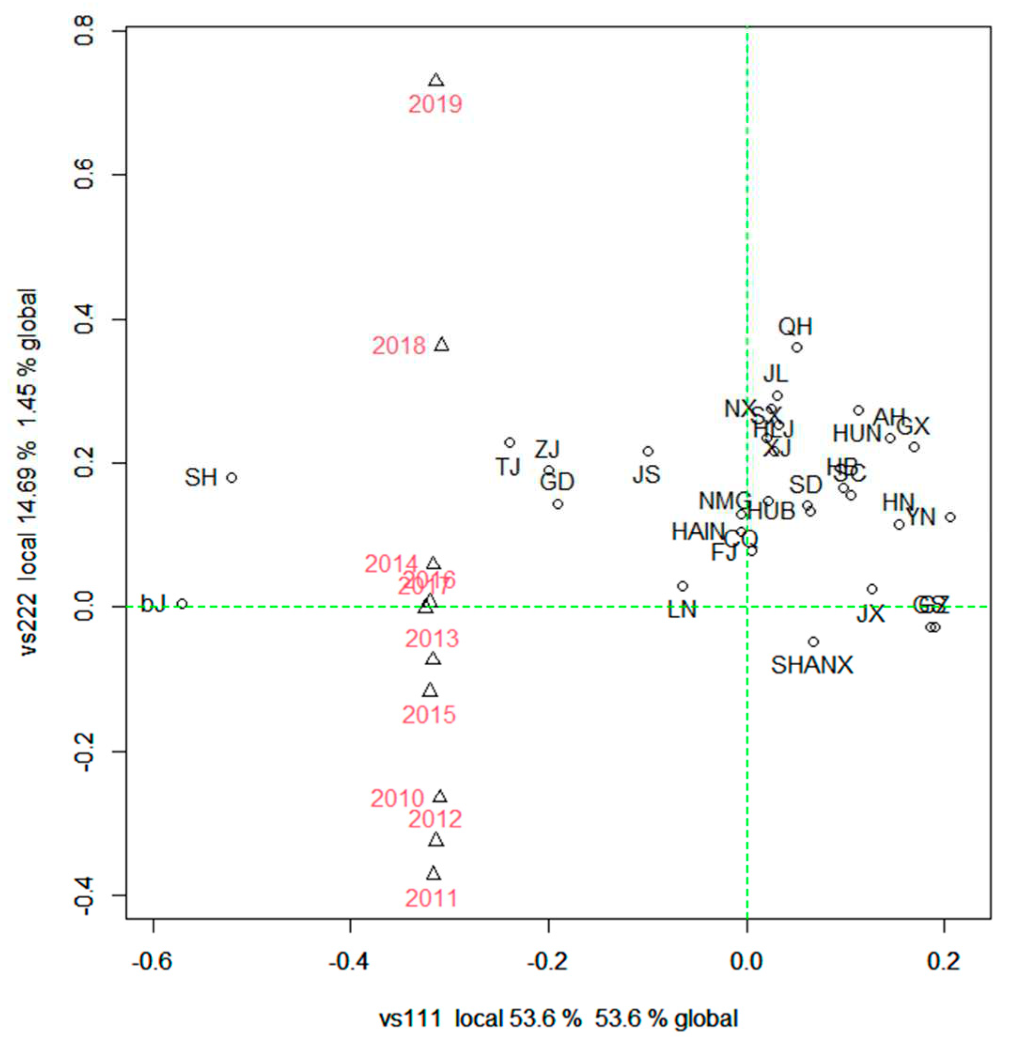
Figure 2. Employment quality scores in 2011, 2014, 2017 and 2020.

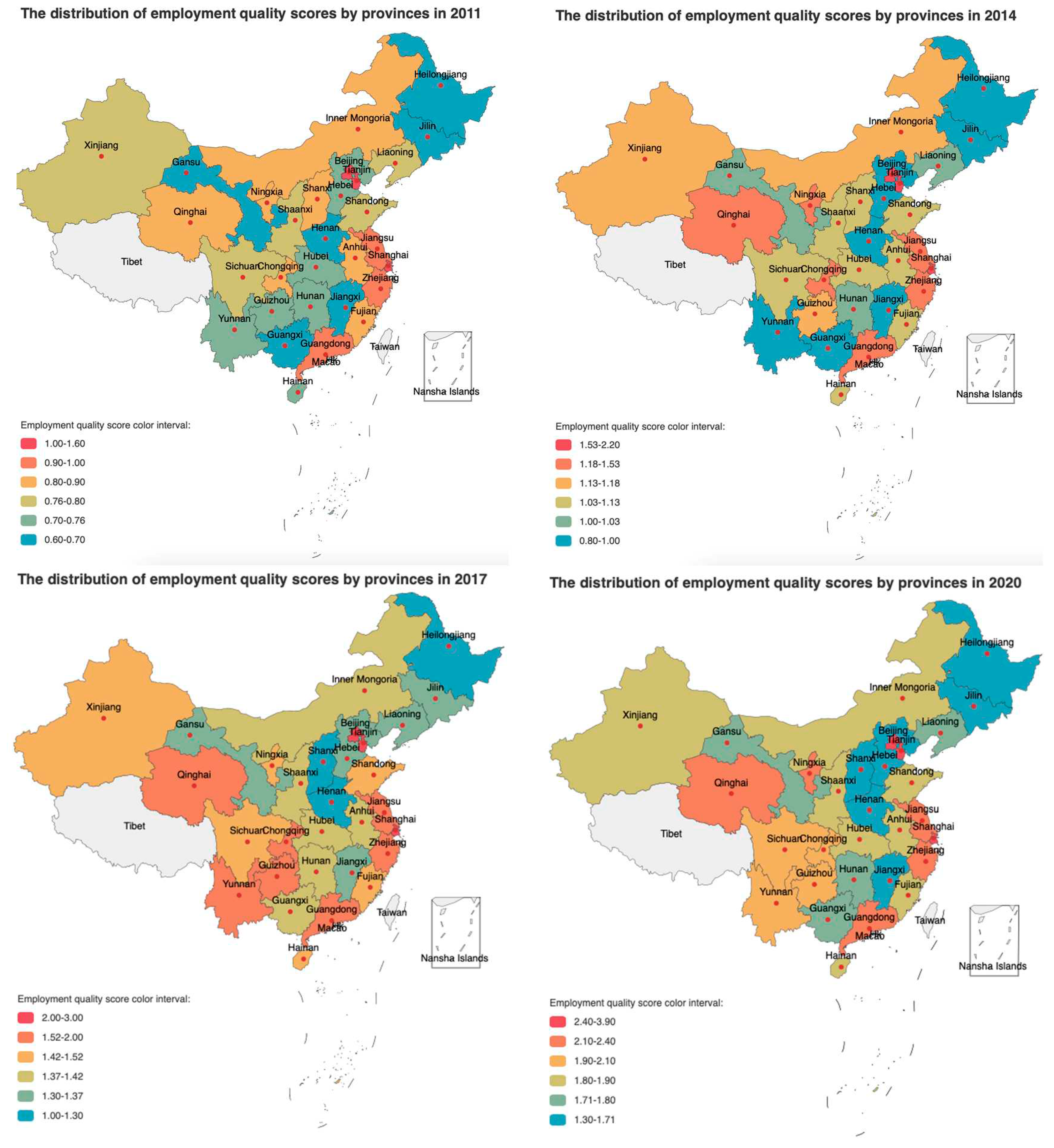
Figure 3. Change trend of employment quality score in time and region.

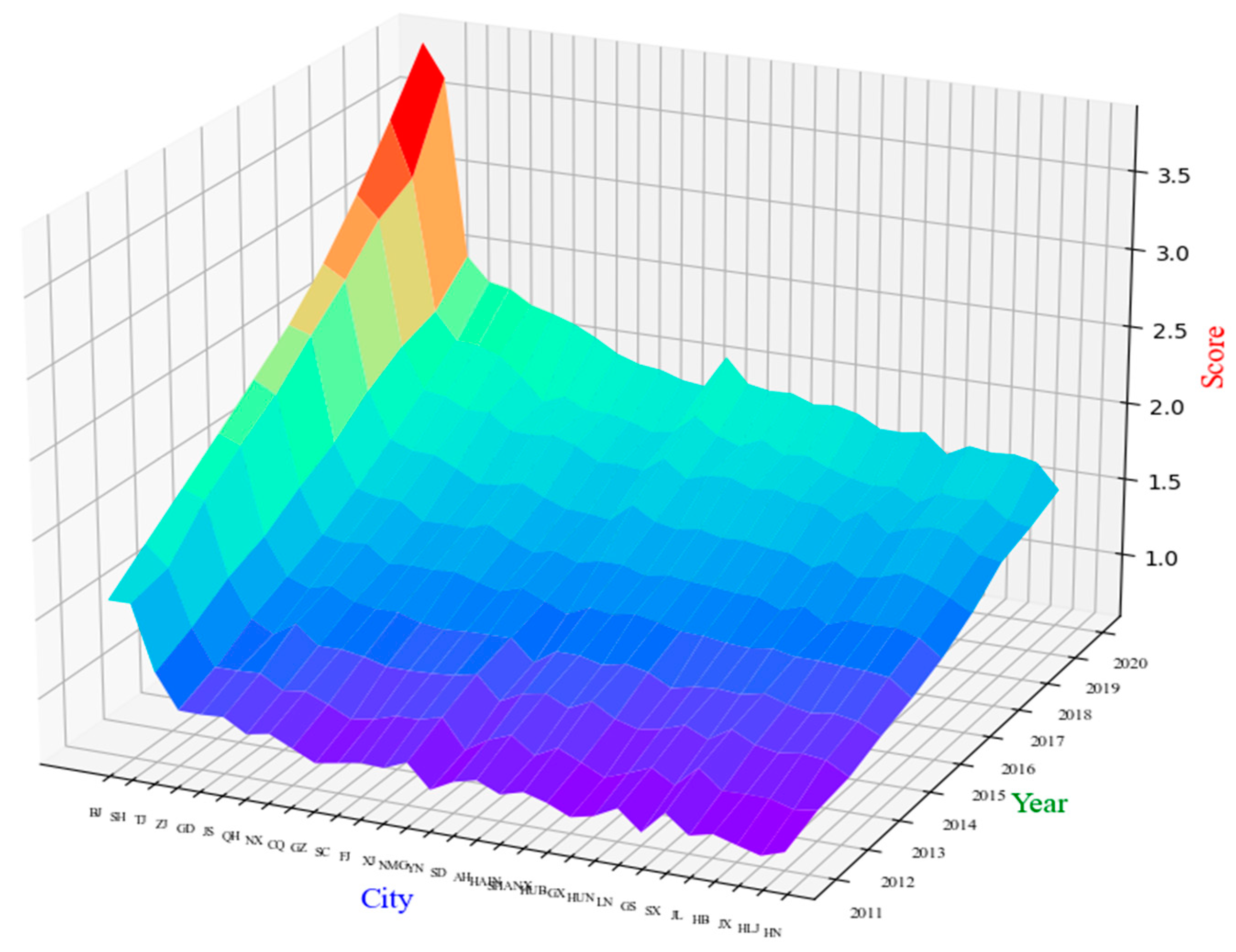
Figure 4. The change of employment quality score ranking from 2020 to 2011.

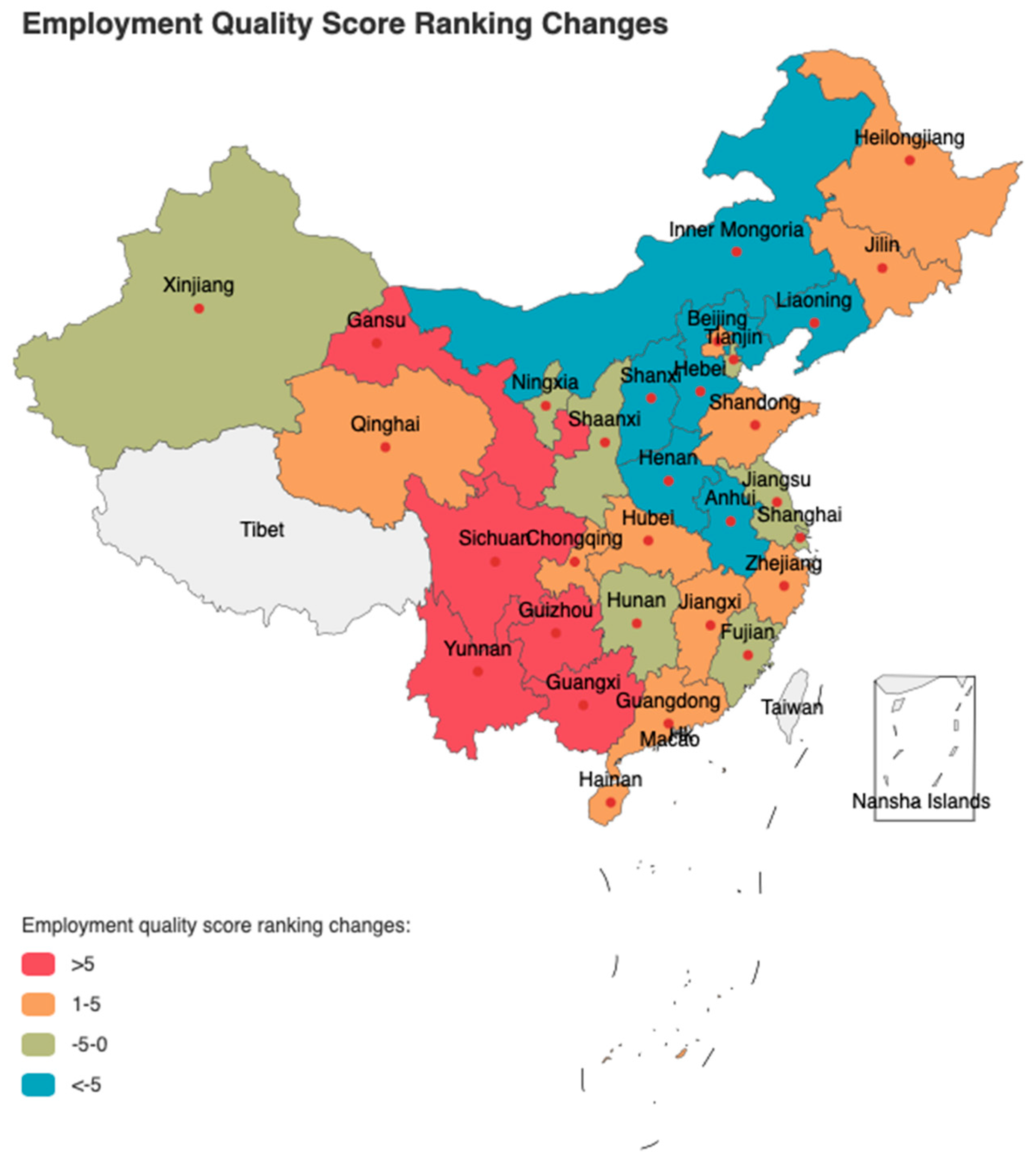
Table 1. Results of interprovincial employment quality evaluation in China.

City	2011	2012	2013	2014	2015	2016	2017	2018	2019	2020
BJ	1.5700	1.7625	1.9550	2.1505	2.3517	2.5529	2.8075	3.1163	3.4690	3.8480
SH	1.5722	1.6363	1.9026	2.0928	2.2728	2.5062	2.7196	2.9737	3.1067	3.6328
TJ	1.1577	1.2795	1.4324	1.5358	1.6948	1.8263	2.0167	2.1616	2.2462	2.4732
ZJ	0.9394	1.0441	1.1921	1.2991	1.4083	1.5525	1.7188	1.8897	2.0726	2.3235
GD	0.9373	1.0458	1.1151	1.2444	1.3789	1.5152	1.6643	1.8682	2.0567	2.2944
JS	0.9462	1.0533	1.2061	1.2851	1.3977	1.5118	1.6586	1.8010	2.0076	2.2053
QH	0.8605	0.9668	1.0837	1.2022	1.2867	1.4028	1.5917	1.8074	1.8910	2.1661
NX	0.8882	0.9867	1.0854	1.1816	1.2995	1.4107	1.5137	1.7043	1.7459	2.1177
CQ	0.8202	0.9256	1.0611	1.1825	1.2914	1.4015	1.5239	1.7005	1.8002	2.0461
GZ	0.7509	0.8560	1.0209	1.1373	1.3017	1.4491	1.5621	1.7178	1.7324	1.9606
SC	0.7765	0.8806	1.0196	1.1173	1.2587	1.3681	1.4898	1.6734	1.7338	1.9118
FJ	0.8027	0.9262	1.0260	1.1281	1.2213	1.3132	1.4358	1.5863	1.7016	1.8942
XJ	0.7954	0.9272	1.0367	1.1316	1.2669	1.3442	1.4276	1.5954	1.6518	1.8464
NMG	0.8553	0.9684	1.0689	1.1328	1.2037	1.2894	1.4078	1.5724	1.6755	1.8285
YN	0.7073	0.7827	0.9191	0.9942	1.1444	1.3219	1.5289	1.6747	1.8007	2.0440
SD	0.7825	0.8717	0.9912	1.0912	1.2105	1.3220	1.4415	1.5625	1.6939	1.8855
AH	0.8185	0.9277	1.0177	1.0896	1.1850	1.2747	1.4127	1.6055	1.6438	1.8589
HAIN	0.7539	0.8213	0.9479	1.0522	1.2148	1.3012	1.4364	1.6154	1.7101	1.8643
SHANX	0.7934	0.8959	1.0161	1.0841	1.1834	1.2817	1.4025	1.5597	1.6298	1.8105
HUB	0.7515	0.8288	0.9280	1.0532	1.1489	1.2711	1.4088	1.5810	1.6494	1.8257
GX	0.6871	0.7569	0.8868	0.9744	1.1436	1.2529	1.3821	1.5297	1.5905	1.7908
HUN	0.7194	0.8106	0.9130	1.0093	1.1208	1.2512	1.3726	1.5245	1.5456	1.7128
LN	0.7937	0.8707	0.9633	1.0215	1.1120	1.1886	1.3009	1.4370	1.5160	1.7101
GS	0.6676	0.7837	0.8959	1.0081	1.1325	1.2385	1.3669	1.5328	1.5308	1.7343
SX	0.8160	0.9201	0.9863	1.0396	1.1015	1.1434	1.2801	1.4074	1.4465	1.6090
JL	0.6992	0.7989	0.9115	0.9918	1.1009	1.1957	1.3084	1.4623	1.5351	1.6856
HB	0.7345	0.8041	0.8847	0.9618	1.0901	1.1853	1.3574	1.4898	1.5173	1.6630
JX	0.6914	0.8011	0.9065	0.9838	1.0844	1.1953	1.3117	1.4719	1.5333	1.6743
HLJ	0.6512	0.7573	0.8891	0.9575	1.0658	1.1502	1.2478	1.3601	1.4229	1.6424
HN	0.6996	0.7767	0.8071	0.8875	0.9551	1.0405	1.1647	1.3342	1.3991	1.4840

Table 2. Results of third-order principal tensor analysis.

principal tensor	associated dimensions		variable	Singular Value	sum of squares	Variance contribution rate
vs111			1	53.71181	5382	53.603845
30 vs111	10	18	3	4.38544	2925.402	0.357341
30 vs111	10	18	4	3.53146	2925.402	0.23172
10 vs111	30	18	6	23.49385	4782.973	10.255689
10 vs111	30	18	7	18.99458	4782.973	6.703714
18 vs111	30	10	9	3.47483	2911.986	0.224349
18 vs111	30	10	10	2.69446	2911.986	0.134896
vs222			11	8.83796	531.557	1.45131
30 vs222	10	18	13	5.04984	140.484	0.473818
30 vs222	10	18	14	4.41033	140.484	0.361408
10 vs222	30	18	16	5.21672	191.285	0.505652
10 vs222	30	18	17	4.74401	191.285	0.418165
18 vs222	30	10	19	3.64027	105.903	0.246221
18 vs222	30	10	20	2.53229	105.903	0.119147
vs333			21	6.3334	250.104	0.745298
30 vs333	10	18	23	1.55274	44.688	0.044797
30 vs333	10	18	24	0.97085	44.688	0.017513
10 vs333	30	18	26	3.38458	89.183	0.212846
10 vs333	30	18	27	3.19603	89.183	0.189792
18 vs333	30	10	29	4.48806	91.701	0.37426
18 vs333	30	10	30	3.40718	91.701	0.215698

Table 3. Score coefficient of principal tensor in index dimension.

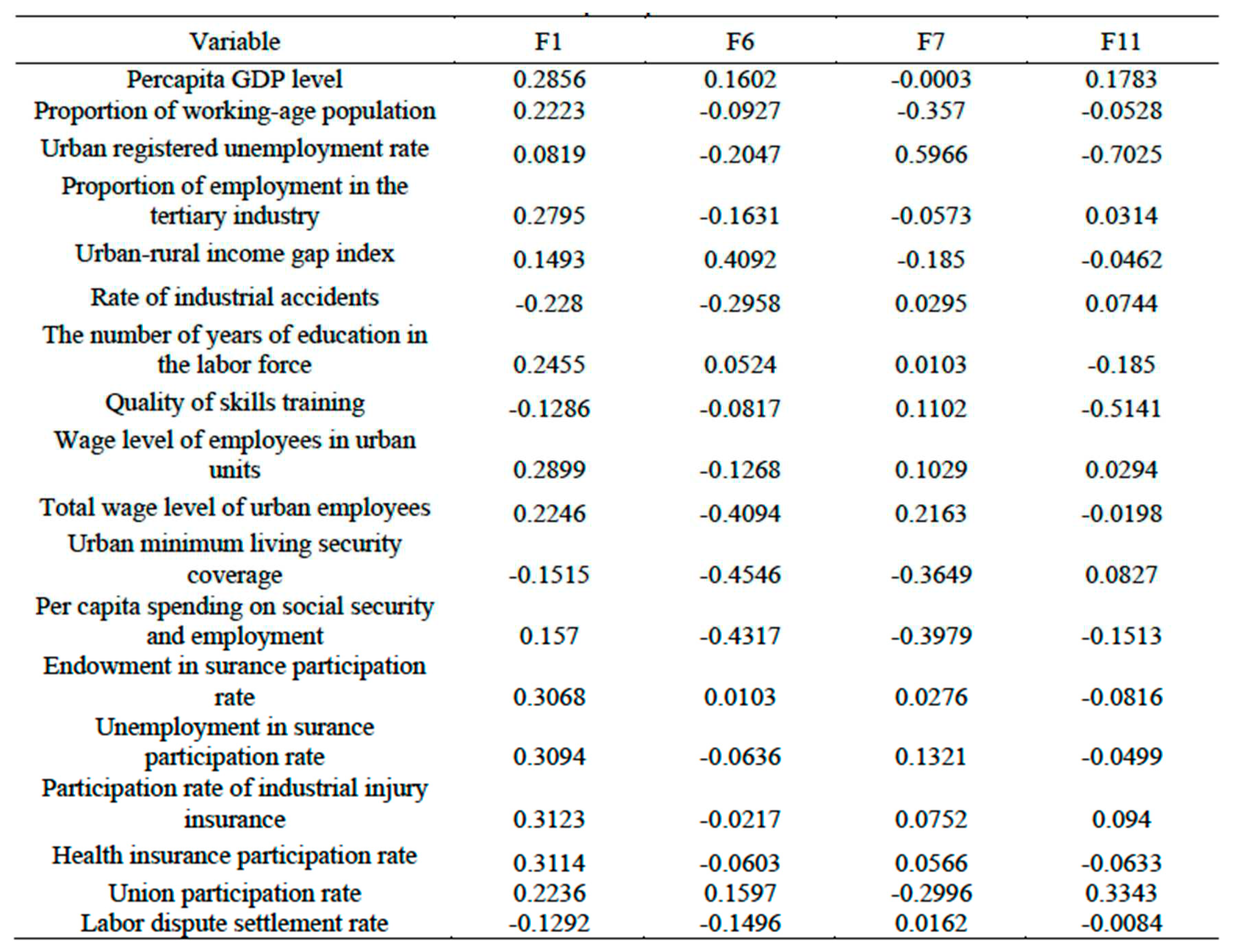
Table 4. Moran's I test of employment quality.

年份	Moran' s I	E(I)	Sd	Z(I)	P-value
2011	0.2538	-0.0357	0.1045	2.7367	0.013
2012	0.2495	-0.0357	0.1109	2.4696	0.024
2013	0.2536	-0.0357	0.1108	2.5105	0.024
2014	0.2347	-0.0357	0.1103	2.3545	0.031
2015	0.2458	-0.0357	0.1110	2.4408	0.030
2016	0.2438	-0.0357	0.1117	2.4118	0.030
2017	0.2634	-0.0357	0.1114	2.5973	0.025
2018	0.2294	-0.0357	0.1108	2.3038	0.033
2019	0.2288	-0.0357	0.1101	2.3038	0.031
2020	0.2068	-0.0357	0.1108	2.0898	0.043

Table 5. Index system of influencing factors of employment quality.

Sort	Index name	Abbreviation	Index interpretation
Explained variable	Employment quality	EQ	Employment quality score
Explanatory variable	Industrial structure	IS	Value added of the primary industry + value added of the secondary industry 2+ Value added of the tertiary industry 3
	Urbanization level	URBAN	Proportion of urban population in total permanent population
	Industrialization level	IL	Per capita industrial output
	Investment policy	IP	Per capita fixed asset investment
	Dependence on foreign trade	DFT	Degree of dependence on imports and exports
	Informatization level	IT	(Number of posts and telecommunications employment in each province/Total population in each province)/(Number of posts and telecommunications employment in the country/total population in the country)
	Price level	PR	Consumer price index
	Fiscal expenditure	FIS	Fiscal expenditure
	Technical level	TFP	Total factor productivity

Table 6. SDM regression results of influencing factors of employment quality in China.

Variable	No fixed effect	Spatial fixed effect	Time-fixed effect	Double fixed effect in space and time
IS	4.0537***	1.0572**	4.1263***	-0.6689*
URBAN	0.4379***	-2.0799***	0.1446	-2.3412***
IL	-0.0234	-0.0275	0.0441	0.0755*
IP	-0.0900**	-0.0049	-0.0916**	0.0624**
DFT	-0.0814***	-0.1537***	-0.0544***	-0.1348***
IT	0.2002***	0.0644**	0.2240***	0.0210
Price	0.6172	-1.7536*	-0.4606	-1.0051
Fiscal	0.0241	0.8284***	0.0110	0.1624**
TFP	0.1563	-0.1060*	0.0785	-0.1035**
W*IS	2.8661***	-1.8073**	4.6846***	-2.4773***
W*URBAN	-0.5106**	2.6290***	-1.2731***	1.2748***
W*IL	-0.0699	0.1505	0.2021**	0.2984***
W*IP	0.1576**	-0.2018***	0.0151	-0.0861*
W*DFT	0.0422	0.1711***	0.0537*	0.0966***
W*IT	-0.1672**	0.1100*	-0.0049	0.1473***
W*Price	-0.3925*	2.8501***	0.1003	-0.0551
W*Fical	0.0753	-0.1922	0.0388	-0.3583***
W*TFP	0.2666	0.0878	-0.1424	-0.1311
W*dep.var.	0.4680***	0.6090***	0.1670**	0.3000***
intercept	-6.9725
R²	0.8968	0.9761	0.9098	0.9862
sigma^2	0.0263	0.0068	0.0237	0.0035
log-likelihood	112.0350	323.6626	127.5496	401.9792

Note: *, **, *** respectively indicate that the variable is significant at the level of 10%, 5%, and 1%.

Table 7. Decomposition of spatial spillover effect of SDM model.

Variable.	Direct effect	Indirect effect	Total effect
IS	-0.8691**	-3.6113***	-4.4804***
UR	-2.3028***	0.7738**	-1.5290***
IL	0.1001**	0.4403***	0.5404***
IP	0.0564**	-0.0938*	-0.0374*
DFT	-0.1304***	0.0747	-0.0557*
IT	0.0326*	0.2093***	0.2420***
PR	-1.0258	-0.5375	-1.5633
FIS	0.1360	-0.4293**	-0.2934*
DFP	-0.1147**	-0.2270*	-0.3418**

Note:“*”,“**”, “***” respectively indicate that the variable is significant at the level of 10%, 5%, and 1%.

Disclaimer/Publisher’s Note: The statements, opinions and data contained in all publications are solely those of the individual author(s) and contributor(s) and not of MDPI and/or the editor(s). MDPI and/or the editor(s) disclaim responsibility for any injury to people or property resulting from any ideas, methods, instructions or products referred to in the content.

© 2024 by the authors. Licensee MDPI, Basel, Switzerland. This article is an open access article distributed under the terms and conditions of the Creative Commons Attribution (CC BY) license (http://creativecommons.org/licenses/by/4.0/).

Copyright: This open access article is published under a Creative Commons CC BY 4.0 license, which permit the free download, distribution, and reuse, provided that the author and preprint are cited in any reuse.

MDPI Initiatives

Important Links

Choose an area of interest and we will send you notifications of new preprints at your preferred frequency.

Disclaimer

Research on the Evaluation and Influencing Factors of China's Provincial Employment Quality Based on Principal Tensor Analysis

Abstract

1. Introduction

2. Literature review

2.1. Research on the measurement of employment quality

2.2. Research on Factors Affecting Employment Quality

3. Research methods

3.1. PTAk Model of k-order Tensor (K>2)

3.2. Global spatial Autocorrelation analysis

3.3. Spatial metering model

4. China’s inter-provincial employment quality measurement and visualization

4.1. Measurement of provincial employment quality in China

4.2. Visualization of employment quality in China's provinces

4.2.1. Expansion and visualization in spatial dimension

4.2.2. Expansion and visualization in time and space dimensions

5. Spatial econometric analysis of influencing factors of employment quality in China's provinces

5.1. Spatial correlation analysis of employment quality in China's provinces

5.2. Analysis of influencing factors of employment quality in China's provinces

5.2.1. Selection of variables and data test

5.2.2. Regression results of spatial Durbin model

5.2.3. Decomposition of spatial effects of factors affecting employment quality in China's provinces

6. Conclusion

Data Availability Statement

References

MDPI Initiatives

Important Links

Subscribe