Preprint
Article

This version is not peer-reviewed.

Collatz Conjecture: Analysis of Binary Structure and Trajectory Behavior

Submitted:

27 August 2026

Posted:

28 August 2026

You are already at the latest version

Abstract

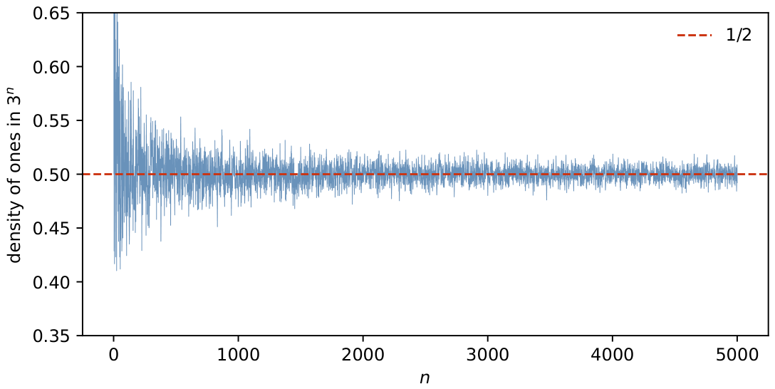
We develop an exact "mantissa" formalism for the binary expansions of natural numbers, in which the gap structure between consecutive ones is encoded by a sequence of fractional parts \(\sigma_j\in(0,1]\). Within this formalism we prove a sharp threshold dichotomy: the next binary gap equals 1 precisely when \(\sigma_j\le \kappa\), where \(\kappa=2-\log_2 3\approx 0.41504\). For \(M=3^n\) we obtain rigorous consequences: an exact characterization of the leading run of ones in terms of \(\{n\log_2 3\}\), whence, by Weyl equidistribution, the asymptotic density of \(n\) whose expansion begins with \(m\) ones equals \(-\log_2(1 - 2^{-m})\), and, by effective bounds for linear forms in logarithms, the leading run has length \(O(\log n)\); and a proof that the trailing run of ones always has length 1 or 2. On the trajectory side, we give an exact decomposition of Collatz iterations, a lemma describing precisely how a block of trailing ones is consumed, and a conditional contraction criterion: if the total 2-adic valuation accumulated along \(M\) odd steps satisfies \(Q_M\ge\beta M\) with \(\beta>\log_2 3\), the trajectory contracts at an explicit exponential rate; conversely, any divergent trajectory must keep \(Q_M\) below \(M\log_2 3+\log_2 X_0\) for every \(M\). The heuristic self-correcting dynamics of the mantissas, together with computations up to \(n=5000\) and valuation statistics over 2000 random trajectories, supports the conjecture that the density of ones in the binary expansion of \(3^n\) tends to \(1/2\); we state this precisely as a conjecture and delimit exactly which steps remain open. We then prove the average-case form of the density statement: for every fixed \(j\ge3\) the \(j\)-th low-order bit of \(3^n\) equals 1 for exactly half of the exponents \(n\) in each period \(2^{j-1}\) (the exceptional positions \(j=0,1,2\) balance to the same mean, so the lowest \(J\) bits carry exactly \(J/2\) ones on average), and the bit at fixed offset \(j\) from the top carries ones with density \(\mu_j\to1/2\) at rate \(2^{-j}\), with \(\mu_1=\kappa\). Thus the outer \(O(\log n)\) digits provably obey the density-\(1/2\) law, and the conjecture is reduced to the middle range of the expansion. We further determine the dispersion and the full asymptotic law of the digit counts in these windows: in the low window the numbers of zeros and of ones each follow an exactly binomial law \(1+\mathrm{Bin}(J-2,\tfrac12)\) over every period—mean \(J/2\), variance \((J-2)/4\), Hoeffding tails, Gaussian local limit—while in the top window the variance equals \(W/4-c_*+O(W2^{-W})\) with \(c_*=0.2399227044\ldots\), and the normalized count of zeros satisfies a central limit theorem. Finally, we identify the natural invariant measure of the gap dynamics itself: in tail coordinates the dynamics is an induced binary shift preserving Lebesgue measure (invariant \(\sigma\)-density \(2^{1-\sigma}\ln2\)), under which the gaps are i.i.d. geometric \(\tfrac12\); for almost every mantissa the density of zeros is \(1/2\) with Gaussian fluctuations of variance \(D/4\), and the density conjecture becomes precisely the assertion that the mantissas of \(3^n\) are typical for this measure—a statement strongly supported by the data (Kolmogorov–Smirnov distance 0.0116 at \(n=2000\)). Moreover, we prove that at every fixed depth \(j\) the interior mantissa \(\sigma_j\) is equidistributed over \(n\), with its law converging to the invariant law at the exponential rate \(2^{-j}/\ln2\); that the gaps decorrelate over \(n\) \((|\operatorname{Cov}(\delta_i,\delta_j)|\le36\cdot2^{-|j-i|})\); and that, consequently, for all \(n\) outside a set of density \(O(1/(\eta^2K))\) the leading segment spanned by the first \(K\) gaps has density of ones within \(\eta\) of \(1/2\). This yields the density conjecture as an asymptotic law on the outer ranges: with windows \(J(n),K(n)\to\infty\) of logarithmic length at both ends of the expansion, the set of \(n\) whose outer segments have ones-density \(\tfrac12+O(\eta)\) has natural density 1. The genuinely open regime is thereby isolated as depths growing linearly with \(n\)—a barrier of the same nature as the classical \(\times2,\times3\) rigidity problems.

Keywords: 
;  ;  

1. Literature Review

The Collatz conjecture, also known as the 3 x + 1 problem, is one of the most famous unsolved problems in mathematics. It posits that for any positive integer N, repeated application of the map (division by 2 if the number is even; replacement by 3 N + 1 if odd) eventually leads to 1. This review summarizes the key contributions of the cited references, focusing on historical context, theoretical advances, computational verifications, statistical properties, and connections with binary representations and integer sequences.

1.1. Historical and Biographical Context

  • Biography of Lothar Collatz [1]: Lothar Collatz (1910–1990) was a German mathematician known for his contributions to numerical analysis. He proposed the conjecture in 1937 while working on graph theory. The problem asks whether the orbit starting from any positive integer M always reaches 1. Despite his 238 publications on numerical methods, this deceptively simple conjecture became his best-known legacy. The conjecture has been verified for all starting values up to 2 71 ( 2.36 × 10 21 ) [34], yet it remains open.
  • Lagarias’ survey [4]: This survey describes generalizations of the conjecture, equivalent formulations (e.g., the Syracuse map on odd integers), and open questions such as the existence of cycles other than ( 1 , 4 , 2 , 1 ) .

1.2. Theoretical Advances

  • Terras [19]: Introduced the stopping-time formalism and proved that the set of N whose trajectory eventually drops below N has natural density 1; the parity vector of the first k steps is determined exactly by N mod 2 k , and all 2 k parity vectors occur equally often.
  • Tao [2]: For any function f ( N ) , almost all orbits (in logarithmic density) attain a minimum value below f ( N ) : orbits are “almost bounded” for almost all N.
  • Krasikov–Lagarias [44]: Density bounds for the set of integers reaching 1, via systems of difference inequalities.
  • Weyl [46]: Equidistribution of the fractional parts { n α } for irrational α (here α = log 2 3 ), which governs the leading mantissa of 3 n = 2 n log 2 3 .
  • Baker [20]: Effective lower bounds for linear forms in logarithms; in particular n log 2 3 C n μ with effectively computable C , μ > 0 , which we use to bound the leading run of ones in 3 n .
  • Stewart [21]: The strongest known rigorous results on digits of exponential sequences; e.g., the number of nonzero digits of 3 n (in any base) grows at least like log n / log log n . The distance between this bound and the conjectured density 1 / 2 measures the difficulty of the digit problem.

1.3. Binary Representations of Powers of 3

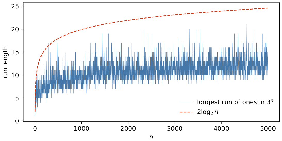
  • MathOverflow question [28]: On the longest run of ones ( L n ) in the binary expansion of 3 n . Simulations up to n = 10000 show L n < 3.5 log n (with an observed maximum of about 24); coin-tossing models predict max L n 2 log 2 N .
  • Cook’s blog [29]: A visualization of the binary expansions of 3 n as a grid whose boundary has slope log 2 3 ; local structures and “semi-chaos” are observed.
  • Wolfram Research [30]: Regularities in the subsequences 3 2 n and 2-adic convergence; the p-adic perspective.

1.3.1. Examples of Binary Expansions

Table 1 lists the binary expansions of 3 n for n = 1 , , 10 .

1.4. Statistical Properties and Computation

  • Sinai [32]: Ergodic properties of the Syracuse map and statistical regularity of long orbits.
  • Barina [33,34]: GPU verification of the conjecture up to 2.95 × 10 20 and then 2 71 .
  • Allouche–Shallit [31]; Everest et al. [45]: Automatic sequences, numeration systems, recurrence sequences, and p-adic limits.

2. Introduction

We study the binary representations of natural numbers—primarily of M = 3 n —through a sequence of fractional parts (“mantissas”) σ j that encode the gaps between consecutive ones. The formalism converts questions about digit patterns into questions about an explicit one-dimensional dynamical system, and it cleanly separates what can be proved from what remains conjectural. Our contributions are the following.
  • An exact mantissa formalism (Section 4): a recurrence and a closed, non-recursive formula for σ j , and a sharp threshold dichotomy (Theorem 4.3): the gap δ j following the j-th one equals 1 exactly when σ j κ , where
    κ = 1 log 2 3 2 = 2 log 2 3 0.4150375 .
  • Rigorous run bounds for 3 n (Section 5): the leading run of ones is characterized exactly by the position of { n log 2 3 } in an explicit interval; Weyl equidistribution then gives the exact asymptotic density log 2 ( 1 2 m ) of exponents n whose expansion opens with m ones, and Baker’s theory gives the effective bound O ( log n ) for the leading run. The trailing run of ones equals 2 for odd n and 1 for even n.
  • Exact trajectory analysis (Section 8): the classical decomposition X = 3 M 2 Q X 0 + b 2 Q , a lemma describing exactly how a block of k trailing ones is consumed by k steps x ( 3 x + 1 ) / 2 , the correct residue classification of the 2-adic valuation ν 2 ( 3 x + 1 ) , and a conditional contraction criterion (Theorem 8.17): accumulated valuation Q M β M with β > log 2 3 forces contraction at rate 2 ( β log 2 3 ) M . We also show that no unconditional bound of the form Q M 2 M O ( 1 ) can hold (Remark 8.18), which delimits precisely where the difficulty of the conjecture lies.
  • The density conjecture and the invariant measure (Section 6): we conjecture that the density of ones in the binary expansion of 3 n tends to 1 / 2 , and we identify the exact dynamical framework behind it: in tail coordinates the gap dynamics is an induced binary shift preserving Lebesgue measure, with invariant σ -density 2 1 σ ln 2 , under which the gaps are i.i.d. geometric ( 1 2 ) and, for almost every mantissa, the density of zeros is 1 / 2 with Gaussian fluctuations of variance D / 4 (Theorem 6.3). Conjecture 6.1 is thereby reduced, exactly, to the typicality of the measure-zero family of mantissas of 3 n (Corollary 6.24); we explain why the known rigorous techniques (Weyl for the leading digit, congruences for the trailing digits, Stewart’s bounds for the digit count) do not yet reach this typicality.
  • Average-case density: rigorous results (Section 7): we prove the n-averaged form of the density statement at both ends of the expansion. For every fixed j 3 , the bit of 3 n at low-order position j is periodic in n with period 2 j 1 and equals 1 for exactly half of each period (Theorem 7.2); the three exceptional positions ( j = 0 : always 1; j = 1 : equal to the parity of n; j = 2 : always 0) balance so that the lowest J bits carry exactly J / 2 ones on average. At the top, the bit at fixed offset j carries ones with density μ j given in closed form, with μ 1 = κ and | μ j 1 2 | 2 j (Theorem 7.3). Beyond the means, we determine the dispersion and the asymptotic law of the measure of the digit counts: in the low window the counts of zeros and ones follow an exactly binomial law with variance ( J 2 ) / 4 and a Gaussian local limit (Theorem 7.4); in the top window the variance is W / 4 c * + O ( W 2 W ) and the normalized counts satisfy a central limit theorem (Theorem 7.7), proved via an exponential memory-loss lemma for the mantissa digits (Lemma 7.6). Conjecture 6.1 is thereby reduced to the middle range of the expansion.
  • Numerical experiments (Section 9): computations up to n = 5000 confirming the dichotomy with zero violations, the density drift toward 1 / 2 , the logarithmic growth of the longest run, and valuation statistics over random trajectories matching the geometric model Pr ( ν = k ) = 2 k .
Throughout, statements labeled Theorem/Lemma/Corollary are rigorous; heuristic arguments are confined to remarks and to Section 6 and are labeled as such.

3. Preliminaries and Method

Zeros drive the Collatz descent: each zero permits a division by 2, outpacing the growth caused by 3 x + 1 . For X 0 = 2 k , the trajectory reaches 1 in exactly k steps. We decompose M into powers of two and track the fractional parts σ j at each stage in order to quantify the structure of gaps between ones.
  • Self-correcting dynamics (informal).
The mantissas σ j induce a self-correcting mechanism that balances ones and zeros: a long run of ones drives the normalized tail up to s 1 2 k , giving a small σ j , and by the dichotomy of Theorem 4.3 the run can persist only while σ stays below κ ; conversely, a run of zeros drives s 0 + , giving σ j 1 , after which gaps of size 1 (ones) reappear. Locally this yields an alternation of blocks; globally, combined with the equidistribution of { n log 2 3 } , it suggests—but does not prove—an asymptotic density of 1 / 2 for the ones in the binary expansion of 3 n (Section 6).

4. The Mantissa Formalism

Definition 4.1
(Binary structure and gaps). Let M N have Hamming weight h (number of binary ones), with the positions of the ones p 0 > p 1 > > p h 1 and gaps δ i = p i p i + 1 , i = 0 , , h 2 . Write M = 2 α 1 + 2 α 2 + + 2 α h in the greedy real-exponent form: α 1 = log 2 M and, recursively, 2 α j + 1 = 2 α j 2 α j . Then α j = p j 1 . Set α j = α j + ϵ j with ϵ j ( 0 , 1 ) , and define the mantissas
σ j = 1 ϵ j + 1 , j = 0 , 1 , , h 1 ,
so that σ j is attached to the one at position p j (for the last one, σ h 1 = 1 ).
Theorem 4.2
(Recurrence for the mantissas). With the notation of Definition 4.1, for every 1 j h 1 ,
M = i = 1 j 1 2 * α i + 2 α j = i = 1 j 2 * α i + 2 α j + 1 ,
and the mantissas satisfy the exact recurrence
σ j 1 = 1 log 2 1 + 2 1 δ j 1 σ j .
For δ j 1 = 1 , the quadratic expansion holds:
σ j 1 = 1 2 σ j 1 ln 2 4 σ j + F j σ j 3 12 , | F j ( x ) | | x |
(Theorem A.1). For δ j 1 > 1 , with the coefficients c 0 , c 1 , c 2 of (A3) evaluated at τ = 2 1 δ j 1 ,
σ j 1 = c 0 + c 1 σ j + 1 2 c 2 σ j 2 + R j ( ln 2 ) 2 σ j 3 8 , | R j ( x ) | | x |
(Theorem A.2).
Proof. 
Identity (4.1) restates the greedy decomposition. Subtracting its two forms,
2 α j = 2 * α j + 2 α j + 1 , hence 2 ϵ j = 1 + 2 α j + 1 * α j = 1 + 2 δ j 1 + ϵ j + 1 .
Taking log 2 and substituting ϵ j = 1 σ j 1 , ϵ j + 1 = 1 σ j gives (2). For δ j 1 = 1 , (2) reads σ j 1 = f ( σ j ) with f ( σ ) = 1 log 2 ( 1 + 2 σ ) ; its Taylor expansion at 0 with the remainder bound of Theorem A.1 gives (4.3). For δ j 1 > 1 we expand f δ ( σ ) = 1 log 2 ( 1 + 2 1 δ σ ) analogously, with the coefficients (A3) and the remainder bound of Theorem A.2.    □
The central structural fact is that the recurrence (4.2) separates the two gap types by an exact threshold.
Theorem 4.3
(Sharp threshold dichotomy). Let κ : = 1 log 2 3 2 = 2 log 2 3 0.4150375 . For every M and every 0 j h 2 ,
δ j = 1 σ j κ , δ j 2 σ j > κ .
Moreover σ j = κ occurs only when δ j = 1 and the ( j + 1 ) -st one is the last ( σ j + 1 = 1 ).
Proof. 
By Theorem 4.8 below, σ j + 1 ( 0 , 1 ] , with σ j + 1 = 1 iff the ( j + 1 ) -st one is the last. If δ j = 1 , then by (4.2) σ j = 1 log 2 ( 1 + 2 σ j + 1 ) , which is increasing in σ j + 1 ; as σ j + 1 ranges over ( 0 , 1 ] , σ j ranges over ( 0 , 1 log 2 3 2 ] = ( 0 , κ ] . If δ j 2 , then 2 1 δ j σ j + 1 2 1 σ j + 1 < 1 2 , so σ j = 1 log 2 ( 1 + 2 1 δ j σ j + 1 ) > 1 log 2 3 2 = κ . The two ranges are disjoint, which proves both equivalences and the boundary case.    □
Corollary 4.4
(Exact inversion for δ j = 1 ). If δ j = 1 , then σ j + 1 = log 2 ( 2 1 σ j 1 ) , and this is well defined exactly on σ j ( 0 , κ ] .
Remark 4.5
(Recursive application of the gap estimates: finite memory and shadowing). Applying the recurrences of Theorem 4.2 deeply —step by step through the expansion—yields two exact mechanisms. (i) Exponentially fading memory. Every backward branch contracts: | f δ / σ | = 2 1 δ σ / ( 1 + 2 1 δ σ ) 1 2 for all δ 1 . Hence m recursive steps determine σ j from the following m gaps alone, up to error 2 m , regardless of the seed: reconstructing σ j with the deliberately wrong seed 1 2 gives maximal errors 2.6 × 10 2 , 4.4 × 10 4 , 3.1 × 10 6 , 1.3 × 10 7 at m = 4 , 8 , 12 , 16 —inside the 2 m envelope. The mantissa is a finite-window function of the gap word. (ii) Shadowing by the quadratic model. Iterating the quadratic recursions (i)–(ii) of Theorem 4.2 in place of the exact ones, the local cubic remainders ( σ 3 / 12 ) are damped by the same factor 1 2 per step, so the total deviation never exceeds twice the largest local remainder: over 25-step stretches of the orbit of 3 2000 the maximal shadowing error is 5.4 × 10 3 . Consequently the dichotomy of Theorem 4.3 becomes a finite-window criterion —the next gap is computable from the following m gaps except when σ j lies within 2 m of the threshold κ, and these boundary cases are exactly the deep gates of Proposition 6.9. This backward contraction is the elementary mechanism behind the transfer-operator contraction of Theorem 6.27 and the decorrelation of Theorem 6.28: the statistical half of this paper is the deep recursive application of the gap estimates, performed once and for all at the level of laws.

4.1. Direct Non-Recursive Relation

Theorem 4.6
(Direct non-recursive relation). Let σ 0 satisfy 2 1 σ 0 = k = 0 h 1 2 i = 0 k 1 δ i . Then for 0 j < h ,
σ j = 1 Δ j log 2 2 1 σ 0 S j , S j = k = 0 j 1 2 i = 0 k 1 δ i , Δ j = i = 0 j 1 δ i ,
equivalently 2 1 σ j = 2 Δ j 2 1 σ 0 S j .
Proof. 
From the definition of σ 0 , splitting the sum at k = j ,
2 1 σ 0 = S j + k = j h 1 2 i = 0 k 1 δ i = S j + 2 Δ j 2 1 σ j ,
since the tail starting at j, renormalized to the position p j , equals 2 1 σ j (Theorem 4.8). Solving for 2 1 σ j and taking log 2 completes the proof.    □
Corollary 4.7
(Case M = 3 n ).  S j = k = 0 j 1 2 p k n log 2 3 , where p k are the positions of the ones and p 0 = n log 2 3 . Moreover
σ 0 = 1 { n log 2 3 } ,
so the leading mantissa is governed by the equidistribution of { n log 2 3 } [46].
Proof. 
3 n = 2 n log 2 3 , so α 1 = n log 2 3 , ϵ 1 = { n log 2 3 } and σ 0 = 1 ϵ 1 . The formula for S j follows from p 0 = n log 2 3 .    □
Theorem 4.8
(Normalized tail form). For 0 j h 1 ,
2 1 σ j = 1 + s j , s j : = k = 1 h j 1 2 i = 0 k 1 δ j + i [ 0 , 1 ) ,
equivalently σ j = 1 log 2 ( 1 + s j ) ( 0 , 1 ] , with σ j = 1 iff j = h 1 .
Proof. 
The tail at position j consists of the one at p j (contributing 1 after normalization by 2 p j ) plus the contributions of the subsequent ones, each normalized by the accumulated gaps: 2 p j + k p j = 2 Δ k ( j ) with Δ k ( j ) = i = 0 k 1 δ j + i k . Hence s j k 1 2 k = 1 , with equality impossible for a finite expansion, so s j [ 0 , 1 ) and σ j ( 0 , 1 ] . The empty tail ( j = h 1 ) gives s j = 0 , σ j = 1 .    □
Lemma 4.9
(General tail decomposition). For fixed j and any m 1 with j + m h 1 ,
s j = k = 1 m 2 Δ k ( j ) + 2 Δ m ( j ) s j + m .
Proof. 
Split the sum defining s j at k = m ; the second part equals the tail at j + m shifted by Δ m ( j ) : k = m + 1 h j 1 2 Δ k ( j ) = 2 Δ m ( j ) l = 1 h j m 1 2 Δ l ( j + m ) = 2 Δ m ( j ) s j + m .    □
Corollary 4.10
(Block of ones). If δ j = = δ j + m 1 = 1 , then s j = 1 2 m + 2 m s j + m .
Corollary 4.11
(Small tail). If s j 1 , then σ j = 1 s j ln 2 + s j 2 2 ln 2 + O ( s j 3 ) .
Proof. 
σ j = 1 ln ( 1 + s j ) / ln 2 and ln ( 1 + s ) = s s 2 / 2 + O ( s 3 ) .    □

5. Runs of Ones: Rigorous Bounds

5.1. A Run of Ones Forces a Small Mantissa

Lemma 5.1
(Run compression). If δ j = = δ j + m 1 = 1 (a run of m + 1 consecutive ones starting at p j ), then
s j 1 2 m and hence σ j log 2 1 2 m 1 < 2 m ln 2 .
Proof. 
By Corollary 4.10 and s j + m 0 , s j 1 2 m . Then σ j = 1 log 2 ( 1 + s j ) 1 log 2 ( 2 2 m ) = log 2 ( 1 2 m 1 ) . Finally, ln ( 1 x ) x / ( 1 x ) gives, with x = 2 m 1 1 4 , log 2 ( 1 2 m 1 ) 4 3 · 2 m 1 / ln 2 < 2 m / ln 2 .    □
Thus a long run of ones is possible only where the mantissa is exponentially close to 0: runs are “expensive” in the σ -dynamics.
Remark 5.2
(The potential D j = log 2 ( 1 s j ) ). Lemma 5.1 admits a compact “sum-form” packaging. Since the tail sum satisfies s j < 1 strictly , the quantity D j : = log 2 ( 1 s j ) is finite, and three exact facts hold (each verified on all 388 ones-runs of 3 2000 ): (i) the estimate —every run of ones starting at index j has length at most D j (this is Lemma 5.1 read backwards: the gap of the sum below 1 budgets the run); (ii) additivity —across a run of length m, the potential decreases by exactly the consumed length, D j = m + D j + m (Corollary 4.10 in logarithmic form); (iii) the floor —by integrality, 1 s j 2 p j , i.e., D j p j : the potential never exceeds the remaining length, which is the termination bound of Proposition 10.23 in sum form. The potential D j is, once more, the gate depth toward the round number above the tail: one quantity, four guises—tail deficit, run budget, gate depth, and distance to termination.
For the leading run of 3 n this cost can be converted into rigorous statements, because σ 0 is explicitly 1 { n log 2 3 } by (4.5).

5.2. The Leading Run of 3 n : Exact Characterization

Theorem 5.3
(Leading run). Let m 1 . The binary expansion of 3 n begins with at least m ones if and only if
{ n log 2 3 } log 2 ( 2 2 1 m ) , 1 .
Consequently:
1.
(Density; Weyl) The set of n for which 3 n opens with at least m ones has natural density
d m = 1 log 2 2 2 1 m = log 2 1 2 m = 2 m ln 2 + O ( 4 m ) .
2.
(Effective bound; Baker) There are effectively computable constants C , μ > 0 such that the leading run m ( n ) of 3 n satisfies
m ( n ) μ log 2 n + C ( n 2 ) .
Remark 5.4
(Attribution). Both parts are instances of classical principles and we claim no novelty for the mechanism. Part (1) is the base-2 significant-digit (Benford) law: the density log 2 ( 1 2 m ) equals log b ( 1 + 1 / D ) with b = 2 and D = 2 m 1 , and the Benford property of a n in base b for log b a irrational goes back to Diaconis [13]; see Berger–Hill [14] for the general m-digit law. Part (2) is the standard Baker consequence, equivalent to an effective lower bound for | 2 x 3 y | in the circle of Pillai’s problem. The mirror statement—leading ternary digit strings of 2 n , with the same two ingredients—was obtained independently and simultaneously by Ren and Roettger [6]; our Theorem 5.3 is the base-swapped instance, and we record it here only because the interval characterization (5.1) is what feeds the mantissa formalism of Section 7.
Proof. 
Write 3 n = 2 p 0 + ϵ with p 0 = n log 2 3 and ϵ = { n log 2 3 } ( 0 , 1 ) . The top m bits of 3 n are the first m bits of the real number 2 ϵ ( 1 , 2 ) ; they are all ones iff 2 ϵ 2 2 1 m , i.e., iff (5.1) holds (the right endpoint is never attained since log 2 3 is irrational). (1) By Weyl’s theorem [46], { n log 2 3 } is equidistributed mod 1, so the density equals the length of the interval in (5.1). (2) If 3 n opens with m 2 ones, then by (5.1), 1 ϵ log 2 ( 1 2 m ) 2 1 m , so the distance from n log 2 3 to the nearest integer satisfies n log 2 3 2 1 m . By Baker’s theory of linear forms in logarithms [20], n log 2 3 C 0 n μ with effective C 0 , μ > 0 . Combining, 2 1 m C 0 n μ , i.e., m 1 + log 2 ( 1 / C 0 ) + μ log 2 n .    □
Proposition 5.5
(The continued fraction of log 2 3 writes the top of 3 n ). Let α = log 2 3 , with continued fraction and convergent denominators
α = [ 1 ; 1 , 1 , 2 , 2 , 3 , 1 , 5 , 2 , 23 , 2 , 2 , 1 , 1 , 55 , ] , q k = 1 , 1 , 2 , 5 , 12 , 41 , 53 , 306 , 665 , 15601 ,
Then:
1.
The leading ones-run of 3 n has length log 2 ( 1 ε n ) + O ( 1 ) and the zeros-run following the leading one has length log 2 ε n + O ( 1 ) , where ε n = { n α } ; hence the records of the leading structure over n N occur exactly at the one-sided best-approximation denominators of α—the convergents and semiconvergents—with sizes log 2 q k + 1 + O ( 1 ) , the side (ones vs. zeros) alternating with the parity of the convergent.
2.
Verification: at n = q 9 = 15601 the leading ones-run is 15 against log 2 q 10 = 15.0 ; at n = q 8 = 665 the post-leading zeros-run is 14 against log 2 q 9 = 13.9 ; at n = q 7 = 306 the ones-run is 9 against 9.4 ; the full record list over n 2 × 10 4 is n = 5 , 12 , 53 , 359 , 665 , 14204 —convergents and semiconvergents only. The large partial quotients of α (23, then 55) are directly visible as the long plateaus between records ( 665 15601 ).
3.
Consequently, the effective irrationality theory of α and the leading-run bound of Theorem 5.3(2) are the same statement in two languages: q k + 1 q k μ (Baker–Feldman) ⇔ leading structure μ log 2 n + O ( 1 ) . The binary expansion of the single constant log 2 3 —through its continued fraction—literally writes the extremal top of every 3 n .
Proof. (1) is Theorem 5.3’s interval characterization combined with the classical theory of one-sided best approximations (the minima of 1 ε n and of ε n over n N are attained at convergents and semiconvergents, with q k α 1 / q k + 1 ) [22]. (2) is direct computation. (3) restates (1) at n = q k .    □
Remark 5.6
(The sequence { n log 2 3 } under the microscope). Direct examination of the governing sequence confirms and completes the picture. (i)The three-distance theorem holds as it must: the sorted points { n α } , n N , exhibit exactly 2 or 3 distinct gap lengths at every tested N. (ii) The star discrepancy is minimal precisely at the convergent denominators: N · D N = 1.00 at N = 665 and N = 15601 , against 3.10 at N = 2000 and 6.44 at N = 20000 . This resolves an apparent paradox: the record leading runs occur at exactly those N where the sequence is best distributed—a single point coming extremally close to 0 or 1 is the signature of optimal global uniformity, not a violation of it. (iii) The classical identity q k α · q k + 1 1 is confirmed to 2 % at q k = 53 , 306 , 665 . (iv) Finally, the binary digits of the constant log 2 3 itself are empirically balanced ( 47.1 % ones in the first 240 bits, longest run 9)—but the normality of log 2 3 is an open problem. The self-similarity thus closes at the top: the digit statistics of 3 n are governed by a constant whose own digit statistics are unproven, and both questions belong to the same × 2 , × 3 circle.
Remark 5.7
(How many times is the extreme attained?). Optimal global uniformity indeed forces the extreme approaches to be essentially unique, at both levels. (i) Over the family: classically, for every N there is at most one n N with n α < 1 / ( 2 N ) (uniqueness of the best approximation; verified: counts 1 , 1 , 1 , 0 at N = 10 2 , 10 3 , 5 · 10 3 , 2 · 10 4 )—the record top approach over any range is attained once, at the (semi)convergent. (ii) Along the orbit of a fixed n: the number of gate passages within one binade of the deepest is 1 for 57 % of sampled exponents and 2 for a further 25 % —“once or twice” in 82 % of cases, with a geometric tail, exactly as extreme-value theory predicts; and the separation law of Proposition 6.9(2) guarantees that deep passages are isolated in time regardless. The deep tail of the gate process is thus an essentially singular event: provably unique over the family, typically unique or double along each orbit. It is worth locating the source of this uniqueness precisely—and it is best described not as something apart from uniformity, but as the deepest of three levels of one and the same irrationality of α = log 2 3 . Level 1 (averages): the bare irrationality of α is equivalent to equidistribution (Weyl)—this level yields all the mean laws of this paper. Level 2 (fluctuations): the measure of irrationality—the size of the partial quotients—governs the rate of uniformity: the discrepancy satisfies N · D N a i , minimal exactly at the convergent denominators (Remark 5.6); this level yields the window sizes of the quantitative theorems. Level 3 (extremes): the continued-fraction structure itself—the same arithmetic object, read exactly rather than in rate form—yields the best-approximation theorem n α > q k α for n < q k + 1 , n q k , hence the at most one statement; note that level 2 alone would permit up to N · D N 6.4 points in the extremal window at N = 2 × 10 4 , so the extremes genuinely require the third level. Averages, rates, and extremes are thus successively finer readings of the single irrational number α; the pattern that runs through the whole paper is that our theorems occupy levels 1–2 everywhere and level 3 only at the top, and the open middle is exactly the absence of a level-3 statement for the interior of the expansion. Two regimes of “visiting the extreme” must be kept apart. At any fixed depth δ, equidistribution forces infinitely many visits, with density exactly 2 δ (measured: 0.02000 at δ = 0.01 , N = 4 × 10 4 )—finiteness at fixed depth is impossible. At growing depth, the visits thin out to the (semi)convergents: the solutions of n α < n 1.1 up to n = 2 × 10 5 are exactly the fifteen numbers 1 , 2 , 3 , 5 , 7 , 12 , 41 , 53 , 306 , 359 , 665 , 1330 , 1995 , 31867 , 190537 —and whether this list is finite is precisely the statement that the irrationality measure of log 2 3 is 2.1 : conjecturally true, while the proven Baker–Feld’man measure is finite but large. The finiteness of deep visits is thus, already at the top of the expansion, an open level-3 question—the family counterpart of the target ( ) .
Remark 5.8
(Rational approximations of α organize the digit table). Since α = log 2 3 is irrational, its rational structure enters through the convergents p k / q k —and they organize the whole table of gap words ( δ j ( n ) ) as a function of n. Shifting the exponent by a convergent denominator changes the seed by only q k α 1 / q k + 1 , so the top of the expansion—the initial segment of the gap word—is reproduced to depth log 2 q k + 1 . Measured over random exponents: shifts by q = 12 , 53 , 306 , 665 , 15601 reproduce on average 4.8 , 7.4 , 8.3 , 12.8 , 13.8 leading bits against log 2 q k + 1 = 5.4 , 8.3 , 9.4 , 13.9 , 18.5 , while generic shifts ( q = 100 , 500 ) reproduce only 1 bit. The n-direction of the table is thus quasi-periodic with periods the convergent denominators and depths the logarithms of the next ones: to know the top m bits of 3 n one needs n only through its position relative to the q k -lattice with q k + 1 > 2 m . This is the practical content of “writing the irrational α through its rational approximations”: the convergents are the coordinate system of the digit table—its rows were indexed by n, its quasi-periods are the q k , and the local structure everywhere else is governed by the invariant measure.
Remark 5.9
(The budget deficit is the Diophantine distance). The convergent denominators, the gaps, and the sub-unit budget of Theorem 4.8 are linked by one exact asymptotic. Writing ε = { n α } and u = n α : on the zeros side (ε small) the tail sum itself is the distance, s 0 = 2 ε 1 = ( ln 2 ) u ( 1 + o ( 1 ) ) , whence the first gap is δ 0 = log 2 ( 1 / u ) log 2 ln 2 + o ( 1 ) ; on the ones side (ε near 1) the deficit below the budget is the distance, 1 s 0 = 2 2 ε = ( 2 ln 2 ) u ( 1 + o ( 1 ) ) , whence the potential is D 0 = log 2 ( 1 / u ) log 2 ( 2 ln 2 ) + o ( 1 ) . At n = q k , where u 1 / q k + 1 , the extreme leading block therefore has length log 2 q k + 1 + c with c = + 0.53 or 0.47 according to the side, which alternates with the parity of k. Measured: at n = 665 the ratio s 0 / ( ( ln 2 ) u ) equals 1.0000 and δ 0 = 14.48 against the predicted 14.46 ; at n = 306 the ratio ( 1 s 0 ) / ( ( 2 ln 2 ) u ) equals 0.9995 and D 0 = 8.93 against 8.91 ; at n = 41 : 0.9943 and 5.46 against 5.26 . Thus q k + 1 is, up to the constant ln 2 , the reciprocal of the budget deficit at n = q k : the continued-fraction ladder of α and the sub-unit budget of the expansion are one object seen from two sides, and the “sum < 1 ” of the tail is, at the top, literally the irrationality of log 2 3 made quantitative.
Remark 5.10
(Counts at the convergents: the division of labor). The triangle q k + 1 δ  counts closes with each vertex governed by its own level. (i) The numerators count the digits: at n = q k the total digit count is the convergent numerator , L ( q k ) = p k + { 0 , 1 } exactly, the extra unit alternating with the side—measured: L = 20 , 65 , 85 , 485 , 1055 , 24727 against p k = 19 , 65 , 84 , 485 , 1054 , 24727 at q k = 12 , 41 , 53 , 306 , 665 , 15601 . (ii) The ladder barely touches the split: the deterministic contribution of the extreme block to the balance W = Z h is only log 2 q k + 1 ( 5.7 , , 18.5 at the tested q k ), while the measured balances W = 13 , + 15 , 23 , + 33 , + 153 sit at the diffusive scale 2 h = 8.8 , 8.4 , 22.5 , 32 , 157 —an order larger. (iii) The division of labor: the extremes of the expansion (deepest blocks, records) belong to the continued fraction of α; the counts of zeros and ones belong to the invariant measure; and the two meet only at the O ( log ) level, invisible against the O ( n ) fluctuations of the counts. This is the final shape of the hierarchy: the ladder writes the extremes, the measure writes the averages, and the conjecture is that nothing else writes anything.
Remark 5.11
(Run compression as a density mechanism). Theorem 5.3(1) can also be derived directly from Lemma 5.1: a leading run of m + 1 ones forces σ 0 < 2 m / ln 2 , and since σ 0 = 1 { n log 2 3 } is equidistributed [46], the density of such n is at most 2 m / ln 2 —matching the exact value log 2 ( 1 2 m ) = 2 m / ln 2 + O ( 4 m ) up to the error term. The same mechanism operates at every interior index j: a run of m + 1 ones starting at j occurs only on the exponentially small set { σ j < 2 m / ln 2 } . For fixed j the distribution of σ j over n is in fact provable—see Theorem 6.27, which combines the same Weyl mechanism with the transfer operator of the shift; what remains unproven is uniformity in j growing with n (Remark 6.31). Subsection 6.1 identifies the invariant measure that governs the deep-j regime for almost every mantissa and empirically governs it for 3 n .
Remark 5.12
(Interior runs). Lemma 5.1 applies to interior runs as well: a run of m + 1 ones starting at index j forces σ j < 2 m / ln 2 . However, for j 1 the quantity σ j is not directly expressed through n log 2 3 , so no analogue of Theorem 5.3(2) for interior runs is currently available; the observed logarithmic growth of the longest interior run (Section 9, Figure 3) matches the coin-tossing model [28] but remains conjectural.

5.3. The Trailing Run of 3 n

Lemma 5.13
(Trailing run). For n 1 , 3 n 3 ( mod 8 ) if n is odd and 3 n 1 ( mod 8 ) if n is even. Consequently the trailing run of ones in the binary expansion of 3 n has length exactly 2 for odd n and exactly 1 for even n; in particular it never exceeds 2.
Proof. 
3 2 = 9 1 ( mod 8 ) , so 3 n mod 8 alternates between 3 and 1. If n is odd, the last three bits are 011: a trailing run of exactly two ones. If n is even, the last three bits are 001: a trailing run of exactly one one.    □

5.4. Pointwise Bounds: Both Binary Digits Occur Unboundedly Often

For the ones, a pointwise lower bound is classical: Stewart’s theorem [21] gives h ( n ) log n / log log n effectively (since 3 n has a single nonzero ternary digit). For the zeros, the following result provides the pointwise counterpart; to our knowledge it is the natural statement reachable by current methods.
Theorem 5.14
(The number of zeros tends to infinity pointwise). For every k, the set of n such that the binary expansion of 3 n consists of at most k maximal blocks of ones is finite. Consequently the number of blocks, and hence the number Z ( n ) of zeros, tends to infinity as n .
Proof. 
A positive integer whose expansion has at most k blocks of ones can be written as a signed sum of at most 2 k powers of two: each block 2 c + 2 c + 1 + + 2 c + r 1 equals 2 c + r 2 c . Thus if 3 n has at most k blocks,
3 n = i = 1 m ϵ i 2 b i , m 2 k , ϵ i { ± 1 } , b 1 > b 2 > > b m 0 .
Dividing by 3 n yields the S-unit equation i = 1 m ϵ i 2 b i 3 n = 1 with S = { 2 , 3 } . Every nonempty subsum i I ϵ i 2 b i is nonzero, because the term with the largest exponent strictly dominates the rest ( 2 b > b < b 2 b ); hence every solution is nondegenerate. By the finiteness theorem for S-unit equations (Evertse; van der Poorten–Schlickewei) [23], which is ineffective for m 3 because it rests on the quantitative Subspace Theorem, while the two-term case is effective by Baker’s method (see Gyory [16] for the precise dichotomy), there are only finitely many nondegenerate solutions ( x 1 , , x m ) , and each value x i = ± 2 b i 3 n determines the pair ( b i , n ) uniquely by unique factorization. Hence only finitely many n admit at most k blocks. Finally, consecutive blocks are separated by at least one zero, so Z ( n ) ( # blocks ) 1 .    □
Remark 5.15
(Effectivity in the low-weight range, via “few binary digits”). The ineffectivity of Theorem 5.14 disappears entirely in the range of small Hamming weight, where the problem for the specific base 3 has been completely solved. Dimitrov and Howe [38] prove, by elementary congruence methods together with a finite computation, that
h ( 3 x ) 22 x 25 .
Thus every equation h ( 3 n ) = k with k 22 is settled outright; the complete lists for the smallest weights are
k { n : h ( 3 n ) = k } 1 0 2 1 , 2 3 4 4 3 5 7 6 5 , 6 , 8
and h ( 3 n ) 23 for every n > 25 . We stress that this is a different problem from the one treated by Bennett–Bugeaud–Mignotte [37] and by Corvaja–Zannier [39]: those authors bound the number of binary digits of perfect powers y q , and 3 n is not in general a perfect power, so their theorems do not apply to h ( 3 n ) = k directly. For the block-count problem of Section 5 the operative citation is (5.2).
  • A worked example: five binary digits, and the limit of local methods.
Since (5.2) removes any question of novelty, the remainder of this subsection is included for a different reason. The five-digit case h ( 3 n ) = 5 makes an unusually transparent laboratory for the local-to-global obstruction that governs the whole paper, and in particular Proposition 10.21: one can watch a congruence sieve narrow the solution set to density 10 12 and then stop dead, for a reason that is structural rather than computational. We develop that example in full, and then say exactly where an archimedean input becomes unavoidable. Nothing below is claimed as new; the theorem it approaches is [38].
Lemma 5.16
(Truncation principle). For every L 3 the residue 3 n mod 2 L depends only on n mod 2 L 2 , and h ( 3 n ) h 3 n mod 2 L .
Proof. 
The group ( Z / 2 L ) × is Z / 2 × Z / 2 L 2 and 3 has order exactly 2 L 2 in it, whence the first claim. The second is immediate: the low L binary digits of 3 n are the digits of 3 n mod 2 L .    □
Fix n with h ( 3 n ) = 5 and put L = K + 2 , λ K ( n ) = 3 n mod 2 L . By Lemma 5.16 the word λ K ( n ) is determined by n mod 2 K , and
3 n = λ K ( n ) + 2 x 1 + + 2 x t , t = 5 h ( λ K ( n ) ) , x 1 > > x t L .
Thus each residue class n r ( mod 2 K ) carries its own S-unit equation with a known constant term, and a class is eliminated as soon as (5.3) is unsolvable modulo one auxiliary integer. Two constraints are available for free. Reducing (5.3) modulo 3 and using 2 1 gives
λ K ( n ) + i = 1 t ( 1 ) x i 0 ( mod 3 ) ,
a condition on the parities of the free exponents; and for a prime p whose order ord p ( 3 ) divides 2 K the left side of (5.3) is a known residue modulo p, so the reachable set of right-hand sides can be enumerated.
Proposition 5.17
(Elementary reduction modulo 16). If h ( 3 n ) = 5 then n 0 , 4 or 7 ( mod 16 ) .
Proof. 
Take K = 4 , L = 6 ; the sixteen classes give the words λ 4 ( n ) = 3 n mod 64 listed in Table 2. Three mechanisms suffice.
(i) Saturation. For n 11 ( mod 16 ) one has λ 4 = 59 = 111011 2 with h = 5 , so t = 0 and (5.3) forces 3 n = 59 , which is false.
(ii) Parity. For n 3 ( mod 16 ) , λ 4 = 27 and t = 1 , so (5.4) reads ( 1 ) x 1 0 ( mod 3 ) : impossible.
(iii) Auxiliary primes. We use p = 5 and p = 17 , both with ord p ( 3 ) 16 . Modulo 5 one has 2 a 1 , 4 for even a and 2 a 2 , 3 for odd a. Apply (5.3) first at K = 2 : for n 1 ( mod 4 ) we have λ 2 = 3 and for n 2 ( mod 4 ) we have λ 2 = 9 , in both cases t = 3 , and (5.4) forces the three free exponents to share a parity. In both cases λ 2 3 n ( mod 5 ) (namely 3 3 and 9 4 ), so (5.3) demands 2 x 1 + 2 x 2 + 2 x 3 0 ( mod 5 ) ; but the threefold sums lie in { 1 , 2 , 3 , 4 } in either parity and never vanish. Hence n ¬ 1 , 2 ( mod 4 ) , which disposes of the eight classes 1 , 2 , 5 , 6 , 9 , 10 , 13 , 14 modulo 16.
For n 15 ( mod 16 ) we have λ 4 = 43 , t = 1 ; (5.4) forces x 1 odd, and 43 + 2 x 1 0 , 1 ( mod 5 ) , whereas 3 n 2 ( mod 5 ) . For n 8 and n 12 ( mod 16 ) we use p = 17 , where 2 a { 1 , 4 , 13 , 16 } for even a and 2 a { 2 , 8 , 9 , 15 } for odd a. In the first case λ 4 = 33 16 , t = 3 , the exponents share a parity by (5.4), and 3 n 16 , so one would need a threefold sum 0 ( mod 17 ) : the admissible sums exhaust { 1 , , 16 } and omit 0. In the second case λ 4 = 49 15 , t = 2 , (5.4) forces both exponents even, and 3 n 4 would require a twofold sum 6 ( mod 17 ) , whereas the admissible sums are { 0 , 2 , 3 , 5 , 8 , 9 , 12 , 14 , 15 } .
Every class other than 0 , 4 , 7 is covered, which proves the claim.    □
Theorem 5.18
(Two-adic valuation in the even case). If n is even and h ( 3 n ) = 5 then ν 2 ( n ) = 2 . In particular n 4 ( mod 8 ) , and the class n 0 ( mod 16 ) of Proposition 5.17 is empty.
Proof. 
Let e = ν 2 ( n ) 1 . By the lifting-the-exponent identity ν 2 ( 3 n 1 ) = ν 2 ( 2 ) + ν 2 ( 4 ) + ν 2 ( n ) 1 = 2 + e for even n, so
3 n = 1 + 2 2 + e + 2 A + 2 B + 2 C , A > B > C > 2 + e ,
the position 2 + e of the second digit being determined by n. Fix an even Λ and let M be the largest divisor of 2 Λ 1 coprime to 3; then 2 X mod M depends only on X mod Λ . Writing ω = ord M ( 3 ) and v = ν 2 ( ω ) , put
K ( ρ ) = k Z / ω : 3 k 1 + 2 2 + ρ + 2 a + 2 b + 2 c ( mod M ) for some a , b , c obeying ( ) .
A solution with ν 2 ( n ) = e requires n 2 e ( mod 2 e + 1 ) and n mod ω K ( e mod Λ ) ; these are compatible only if some k K ( e mod Λ ) has ν 2 ( k ) = e (when e < v ) or ν 2 ( k ) v (when e v ). The latter criterion depends on e only through e mod Λ , so a finite computation settles all e at once. For Λ = 24 one gets M = 1864135 , ω = 240 , v = 4 : no ρ admits ν 2 ( k ) 4 , and among e < 4 only e = 2 survives. The independent choice Λ = 48 ( M = 31274997412295 , ω = 26880 , v = 8 ) gives the same verdict.    □
Theorem 5.19
(How far the sieve reaches). Put
N = 2 616 399 878 400 = 2 8 · 3 3 · 5 2 · 7 · 11 · 17 · 43 · 269 .
If h ( 3 n ) = 5 then
n 4 or n 7 ( mod N ) ,
a set of density 2 / N < 7.7 · 10 13 . Moreover, writing the two equations of (5.3) at K = 4 as
3 n = 11 + 2 A + 2 B ( n 7 ) , 3 n = 17 + 2 A + 2 B + 2 C ( n 4 ) ,
the exponent gaps satisfy
A B 4 ( mod 332640 ) ( n 7 ) , ( A B , B C ) ( 1 , 0 ) , ( 0 , 1 ) or ( 1 , 1 ) ( mod 6 983 776 800 ) ( n 4 ) .
Proof. 
By Proposition 5.17 and Theorem 5.18 we may assume n 4 or 7 ( mod 16 ) . Fix such an r, let Λ be even, M the largest divisor of 2 Λ 1 prime to 3, ω = ord M ( 3 ) . Since λ 4 ( r ) is known and the free exponents in (5.3) enter only through their residues modulo Λ , the set
K = k Z / ω : 3 k λ 4 ( r ) + 2 u 1 + + 2 u t ( mod M ) for some u i obeying ( 5.4 )
is computable, and n must lie in K modulo ω as well as in r modulo 16. For each of Λ = 24 , 36 , 48 , 60 , 72 , 84 the two conditions leave a single class modulo lcm ( 16 , ω ) , namely n r ; the values of lcm ( 16 , ω ) are 240, 432, 26880, 13200, 581040 and 736848, whose least common multiple is N. The statements about the gaps are read off from the same computation: for each admissible Λ one records not only the surviving k but the surviving tuples ( u 1 , , u t ) , and then the differences over all assignments of the u i to A > B > C . For n 7 every even Λ 72 leaves exactly A B ± 4 , and the common refinement over Λ { 8 , 16 , 20 , 22 , 24 , 28 , 32 , 40 , 42 , 44 , 48 , 54 , 56 , 60 , 72 } , of least common multiple 332640, leaves the four values 4, 90724, 241916, 332636; only A B 4 is compatible with A > B and A B < 90724 . For n 4 every even Λ 72 leaves exactly the three pairs displayed, and their common refinement has modulus lcm = 2 5 · 3 3 · 5 2 · 7 · 11 · 13 · 17 · 19 = 6 983 776 800 .    □
Remark 5.20
(Where the sieve stops, and why it must). The residues 4 and 7 are not artefacts of a particular modulus: they are the ghosts of genuine integer solutions of the relaxed system in which the free exponents of (5.3) are allowed to coincide, or to fall below the truncation height. Indeed 3 7 = 11 + 2 11 + 2 7 is a true five-digit representation, while
3 4 = 81 = 17 + 2 5 + 2 4 + 2 4
solves (5.3) for r = 4 with a repeated exponent, even though h ( 3 4 ) = 3 and n = 4 is not a solution of the original problem. Any congruence satisfied by every solution of (5.3) is satisfied by these two integers, so no sieve by auxiliary moduli whatsoever can reduce Theorem 5.19 below two classes. The same phenomenon explains the gap data: the ghost n = 4 has ( A , B , C ) = ( 5 , 4 , 4 ) , whence the three pairs ( 1 , 0 ) , ( 0 , 1 ) , ( 1 , 1 ) , which are exactly the three cyclic shifts of the degenerate assignment.
What the gap statements do achieve is to convert the residual problem into a purely archimedean one. In the odd case one needs only an upper bound A B < 90724 to force A B = 4 , i.e. 3 n = 11 + 17 · 2 B , a two-variable equation that standard lattice reduction settles completely. In the even case one needs A B and B C both below 6.98 · 10 9 ; since A > B > C forces A B 1 and B C 1 , any such bound contradicts the three admissible pairs outright. Bounds of exactly this shape— A B log n —follow from an effective measure of linear independence for log 2 and log 3 together with Baker’s method, so the five-digit case is reachable by an archimedean argument; it is not reachable by any amount of further sieving. This is the same local-to-global gap as Proposition 10.21, in miniature and with every constant explicit. The actual resolution, by different and entirely elementary means, is [38].
Remark 5.21
(Numerical corroboration). A direct scan confirms h ( 3 n ) 22 exactly for n 25 , the maximum 22 being attained at n = 23 , and min 26 n 60000 h ( 3 n ) = 24 , in agreement with (5.2). In particular n = 7 is the only n 60 000 with h ( 3 n ) = 5 , and the next members of the two progressions of Theorem 5.19 exceed 2.6 · 10 12 : the sieve is consistent with the data by a wide margin, and—as Remark 5.20 explains—necessarily fails to see that the two progressions are almost entirely empty.
Remark 5.22
(Effectivity and the remaining gap). Theorem 5.14 is ineffective : the subspace-theorem machinery behind [23] provides no bound on the largest exceptional n, in contrast with the effective leading-run bound of Theorem 5.3(2) and with Stewart’s effective bound for the ones. The pointwise two-sided picture is now symmetric: h ( n ) log n / log log n effectively (Stewart), and Z ( n ) log n / log log n effectively as well (Theorem 5.25, obtained by iterating Baker’s bound block by block)—while empirically both counts grow linearly ( min Z ( n ) = 603 over 800 n < 3000 , attained at n = 812 ). The linked estimates of Proposition 5.23 were verified exactly for all 2 n 3000 ; at n = 2000 they certify Z 287 from R 1 = 10 , against the actual Z = 1596 —the slack measuring precisely the distance between the extremal and the statistical regime. Upgrading either statement to a positive proportion of L n —for instance Z ( n ) ϵ L n for every large n, which by Remark 8.22 would already feed the Collatz-side machinery once ϵ > 1 1 / log 2 3 0.369 (with the corresponding valuation transfer)—is exactly the pointwise problem delimited in Remark 8.55.
Proposition 5.23
(Linked block estimates). For n 2 let B 1 ( n ) , B 0 ( n ) be the numbers of maximal blocks of ones and of zeros in the expansion of 3 n , and R 1 ( n ) , R 0 ( n ) the longest runs of ones and of zeros. Then, exactly and for every n:
1.
B 1 ( n ) = B 0 ( n ) + 1 ;
2.
Z ( n ) B 1 ( n ) 1    and     h ( n ) B 1 ( n ) ;
3.
Z ( n ) L n R 1 ( n ) + 1 1    and     h ( n ) L n R 0 ( n ) + 1 1 .
Proof. (1) The expansion begins with a one (leading bit) and ends with a one ( 3 n is odd), so the blocks alternate 1-block, 0-block, ..., 1-block. (2) Each 0-block contains at least one zero, so Z B 0 = B 1 1 ; each 1-block at least one one. (3) h is the sum of the B 1 ones-run lengths, so h B 1 R 1 ( Z + 1 ) R 1 by (2); with h = L n Z this rearranges to Z L n / ( R 1 + 1 ) 1 . The second inequality is symmetric, using B 0 h .    □
Corollary 5.24
(Reduction of the pointwise problem to interior runs). Any pointwise bound on the longest run of ones transfers to the zeros count: R 1 ( n ) R implies Z ( n ) L n / ( R + 1 ) 1 . In particular:
1.
If R 1 ( n ) C log 2 n for all large n—as is proved for the leading run (Theorem 5.3(2)), predicted for all runs by the coin model, and confirmed by all data (longest run 21 for n 5000 , against 2 log 2 n 24 )—then Z ( n ) n / log n pointwise, a far stronger conclusion than the ineffective Z ( n ) of Theorem 5.14.
2.
Conversely, small digit counts force long runs: Z ( n ) < ϵ L n forces R 1 ( n ) > 1 / ϵ 1 , and h ( n ) < ϵ L n forces R 0 ( n ) > 1 / ϵ 1 ; the two digits are linked exactly as the block structure dictates.
3.
The route has an intrinsic limit worth stating honestly: a density bound Z ϵ L n via (3) alone would need R 1 1 / ϵ 1 , i.e., uniformly bounded runs—false already for ϵ = 0.369 (runs of length 2 are frequent). Quantitatively, the two-sided envelope h / L n [ 1 / ( R + 1 ) , R / ( R + 1 ) ] (with R = max ( R 0 , R 1 ) ) collapses toward 1 2 only as R 1 : at the realistic R = 10 it gives [ 0.09 , 0.91 ] , at R = 4 it gives [ 0.2 , 0.8 ] , and even at the impossibly perfect R = 2 only [ 1 3 , 2 3 ] —never 1 2 . The extremal inequality (3) is tight only for expansions packed into maximal runs; reaching a positive proportion requires the statistical structure (most runs short), not merely a bound on the longest one, and note also that by the identity h + Z = L n the two digits admit only one independent estimate: any lower bound on the zeros is automatically an upper bound on the ones, so the pointwise programme needs exactly one positive-proportion lower bound per digit. Thus the pointwise ladder is: block count (S-units, no rate) → longest interior run ( O ( log n ) conjectured, only the leading case proved) → n / log n zeros → full density (statistical, open).

Block-by-Block Effective Bounds: Iterating Baker Through the Expansion

The reduction of Corollary 5.24 invites the strategy: bound the first block, then the second, and so on—each block being too long producing a Diophantine contradiction. This strategy works, because every run sitting below a known prefix is governed by an effective linear form in three logarithms.
Theorem 5.25
(Effective block-by-block bounds; Stewart-type rate for the zeros). There are effectively computable constants C 1 , c 2 , c 3 > 0 such that for all n 3 :
1.
If the bits of 3 n above the position t form the integer D (a prefix of length = L n t ), then the maximal run (of ones or of zeros) starting at position t 1 has length
m C 1 ( + 1 ) log n .
2.
Consequently, the k-th maximal block of the expansion (counted from the top) has length at most ( 2 C 1 log n ) k , for as long as this is smaller than L n .
3.
Consequently, the number of blocks satisfies B 1 ( n ) c 2 log n / log log n , and therefore, by Proposition 5.23,
Z ( n ) c 3 log n log log n effectively ,
matching Stewart’s effective rate for the ones [21] and upgrading the ineffective Z ( n ) of Theorem 5.14. With Matveev’s explicit constants the bound may be made completely explicit:
Z ( n ) log n 2 log log n + 52.9 1 .
Proof. (1) A run of m ones at positions t 1 , , t m means 3 n mod 2 t [ 2 t 2 t m , 2 t ) , i.e., | 3 n ( D + 1 ) 2 t | 2 t m ; a run of m zeros means 0 < 3 n mod 2 t < 2 t m , i.e., | 3 n D 2 t | < 2 t m . In either case, with Q { D , D + 1 } 2 + 1 ,
3 n Q 2 t 1 2 m Q , hence Λ : = n ln 3 t ln 2 ln Q 2 1 m .
Λ 0 since 3 n Q 2 t (the left side is odd and exceeds Q for t 1 ). By Baker’s theory of linear forms in logarithms [20] (in the explicit form of Matveev), Λ exp C 0 ( ln Q + 1 ) ln n with effective C 0 , and ln Q ( + 1 ) ln 2 ; combining, m C 1 ( + 1 ) log n . Explicitly, Matveev’s theorem for m = 3 logarithms over Q gives the constant 1.4 · 30 6 · 3 4.5 = 1.4319 · 10 11 , and with A 1 = ln 3 , A 2 = ln 2 , A 3 = ln Q ( + 1 ) ln 2 and B 1.585 n one obtains C 1 = 1.5731 · 10 11 ; then ln ( 2 C 1 ) = 26.475 , which yields (5.5) through step (3). (2) Let k be the length of the prefix consisting of the first k blocks; 0 = 0 and the leading block has 1 C 1 log n by (1) with = 1 (prefix “1”; this recovers Theorem 5.3(2)). By (1), k + 1 k + C 1 ( k + 1 ) log n k ( 1 + 2 C 1 log n ) , whence k ( 2 C 1 log n ) k for k 1 , and the k-th block is at most k . (3) The blocks must exhaust the full length: if B 1 ( n ) + B 0 ( n ) = B blocks cover L n n , then ( 2 C 1 log n ) B n , i.e., B log n / log ( 2 C 1 log n ) c 2 log n / log log n ; blocks of ones constitute at least half of all blocks (Proposition 5.23(1)), and Z B 1 1 . We stress that (5.5) is effective but not practical: it first exceeds 1 at log n 125 , that is for n > 10 54 , so it says nothing about any range that can be computed. This is the normal state of affairs for bounds resting on linear forms in logarithms—Dimitrov and Howe [38] record the same phenomenon for Stewart’s bound on the ones, where the analogous threshold exceeds 4.9 · 10 46 —and it is precisely why the ineffective S-unit route and the effective one are both worth recording.    □
Remark 5.26.
The chain in (2) degrades geometrically with the depth k—the price of encoding the prefix into the height of the rational Q. Uniformizing it (a bound m C log n for every block, independent of depth) is exactly what Corollary 5.24(1) would convert into Z ( n ) n / log n ; no such uniform bound is currently known for any k 2 beyond (2). This localizes the pointwise problem yet again: from all interior runs to the dependence of the run bound on the prefix height. Applied to the first three blocks, the chain gives fully effective polylogarithmic bounds: block 1 C log n , block 2 C 2 log 2 n , block 3 C 3 log 3 n —and so on for any fixed depth. The data indicate that the truth is far stronger and uniform: over n 2 × 10 4 , the maximal length of the k-th block equals 15 , 15 , 14 , 17 , 14 , 14 , 15 , 15 for k = 1 , , 8 —about log 2 n at every depth, with no trace of the geometric degradation of the proved chain. Closing the gap between the proved ( C log n ) k and the observed uniform O ( log n ) is the sharpest available formulation of the pointwise problem.
Remark 5.27
(What the theory of linear forms can and cannot give). A literature check delimits the barrier precisely. (a) Proved. The Baker–Matveev bounds carry the product of the logarithmic heights, | Λ | exp ( C h ( Q ) log B ) ; this is what Theorem 5.25 uses, and no proven bound replaces the product by a sum. (b) Conjectured optimum. The Lang–Waldschmidt conjecture [24] predicts the sum form: | a 1 b 1 a m b m 1 | C ( ϵ ) / m B ( | b 1 | | b m | | a 1 | | a m | ) 1 + ϵ , i.e., for our form m ( 1 + ϵ ) + C ( ϵ ) log n . Feeding this into the chain gives k + 1 ( 2 + ϵ ) k + C log n , hence blocks 2 k log n and Z ( n ) log n : even the strongest standard conjecture in the field improves our unconditional rate only by the log log n factor and remains exponentially far from Z n / log n . (c) A structural limit. The coefficient 1 + ϵ on ℓ in Lang–Waldschmidt cannot be improved for general Q: by pigeonhole, the 2 values log 2 Q are 2 -dense, so some Q of height 2 always achieves | Λ | 2 . Consequently the uniform run bound m C log n is not a linear-forms statement at all: it asserts that the specific prefixes of 3 n never realize the pigeonhole extremes—an orbit-specific, normality-type assertion invisible to any estimate over general Q. The barrier is thus the generality, not the strength, of the Diophantine tools. (d) A promising development, and the result of attempting to use it. The arithmetic holonomy bounds of Calegari–Dimitrov–Tang [25] provide a new route to effective Diophantine approximation. Examining what is available as of this writing: their announced effective results cover the two-variable S-unit equation (with applications to irrationality measures of L ( 2 , χ 3 ) and the 2-adic ζ ( 5 ) ), the full development being deferred to future work. The two-variable case corresponds exactly to the rung k = 1 of our ladder—the leading block—which is already effective through Baker–Feldman. What Theorem 5.14 needs is them-term case: an effective bound for | x 1 + + x m 1 | in S-units with S = { 2 , 3 } , for every fixed m; any such result would immediately convert the S-unit argument into an effective block-count rate via the correspondence of Theorem 5.14 (each k-block configuration is a 2 k -term solution). This is, in our view, the sharpest concrete request the present problem addresses to the holonomy program. Meanwhile, the rungs available today can be made numerically explicit: for the leading run, the two-logarithm bounds of Laurent–Mignotte–Nesterenko give m 1 C 0 ( log n ) 2 with modest explicit C 0 , and Feld’man’s refinement of Baker’s theorem gives m 1 κ log 2 n + O ( 1 ) with effective (large) κ; for the chain step, Matveev’s explicit three-logarithm constant applies verbatim to Theorem 5.25.
Remark 5.28
(Composite patterns and the convergent ladder). One may hope that applying the estimates to a composite pattern—say two zeros-blocks flanking a ones-block, 0 g 1 1 m 0 g 2 —produces a stronger simultaneous constraint than the blocks give separately. The exact identities show the opposite: the pattern is equivalent to the nested pair of round-number approximations
| 3 n A | < 2 t g 1 , | 3 n B | 2 t m , B A = 2 t g 1 ,
( A = D 2 t for the zeros-run, B = ( D 2 g 1 + 1 ) 2 t for the ones-run, t = t g 1 ), and closeness to B determines the distance to A: at the record pattern 0 1 1 21 0 2 of 3 4536 , | 3 n A | / ( B A ) = 1.000000 . The conditions form one ladder of dyadic convergents—each block refines the previous approximant—so the composite constraint is exactly the product of the single-block constraints, which is precisely the chain of Theorem 5.25. Improving on the chain therefore requires a bound for the whole word at once; linear forms in many logarithms carry constants growing exponentially in the number of terms, and the subspace machinery is uniform but ineffective—the same trade-off identified in Remark 5.30.
Remark 5.29
(The singular skeleton and the carry involution). The picture assembled above admits a unifying decomposition. Call the countable family of round numbers R = { Q 2 t : Q , t N } the singular skeleton. By the two cases in the proof of Theorem 5.25, every long run is an exponentially close one-sided approach to the skeleton: a run of m ones below the prefix D means 3 n ( D + 1 ) 2 t 2 t m , ( D + 1 ) 2 t —approach from the left; a run of m zeros means 3 n D 2 t , D 2 t + 2 t m —approach from the right; the digit type merely records the side. Adding the single term 2 0 , where 0 is the position of the lowest one of the run, carries 3 n across the skeleton point and exchanges the two sides: for the record run of 3 4536 , the perturbation converts 1110 1 21 00 into 1111 0 22 0 exactly. Correspondingly, the law of the digits decomposes into a continuous bulk and a singular part: within a window of K gaps, the bulk (all runs < m ) carries the absolutely continuous invariant statistics—every asymptotic law of Section 7Section 6 is a bulk statement—while the singular part, the union of one-sided 2 m -neighborhoods of skeleton points, has measure 1 e 2 K 2 m (verified: 0.719 / 0.713 , 0.257 / 0.268 , 0.069 / 0.075 for m = 6 , 8 , 10 at K = 40 ) and contains the entire pointwise difficulty: Baker’s bound of Theorem 5.25 is precisely a bound on the penetration depth into a skeleton neighborhood, with the height of the skeleton point as the price. The decomposition organizes the problem—bulk: solved; skeleton: height-weighted and open—without yet breaking the height barrier.
Remark 5.30
(The linked estimates flow one way). It is natural to hope that the count estimates could be fed back into the machinery—counts bounding runs, runs improving counts, and so on, breaking the prefix-height dependence by bootstrap. The logical flow, however, is one-directional:
run bounds block counts digit counts ,
and the converse implications fail. Rearranging Proposition 5.23(3) gives, from a large Z, only R 1 L n / ( Z + 1 ) 1 —a lower bound on the longest run, not an upper one; and no count information can exclude a long run, because large counts and long runs coexist: at n = 4536 the expansion has Z = 3579 zeros (density 0.498 ), 1819 blocks with a perfectly geometric length distribution ( 902 , 456 , 248 , 111 , )—and simultaneously a run of 21 ones. A single long run costs only O ( log n ) digits and leaves every count statistic intact; this is precisely why the pointwise problem concentrates in the run bound and cannot be recovered from count bootstrapping. The two currently available mechanisms remain: effective linear forms, whose constant degrades with the prefix height (Theorem 5.25), and the ineffective subspace machinery, which requires the number of blocks in the prefix to stay bounded (Theorem 5.14).
Remark 5.31
(No local compensation law). It is tempting to hope that Theorem 4.8, Lemma 5.1 and Theorem 5.3 force a block of ones to be preceded(or followed) by a block of zeros of comparable length—this would immediately give a pointwise density bound. The tail recurrence shows why no such local law can hold: s j 1 = 2 δ j 1 ( 1 + s j ) , so a single zero ( δ j 1 = 2 ) already resets the tail from any value s j 1 (the value just above an arbitrarily long run of ones) to a legitimate s j 1 1 2 . The exponentially small mantissa σ j < 2 m / ln 2 demanded by Lemma 5.1 is produced by the run itself—by the tail 1 + s j approaching 2—not by any preceding zeros; and Theorem 5.3 constrains only the leading run through σ 0 . The correct picture has two levels, and both are visible in the exact identities. At the level of values, adjacent blocks are deterministically and exponentially sharply coupled: s j 1 = 2 δ j 1 ( 1 + s j ) and s j = 1 2 m + 2 m s j + m hold exactly, so a run of m + 1 ones pins the preceding tail to the lattice value 2 1 δ j 1 within 2 m (at the record run of 3 4536 : s j 1 = 0.499999814 , within 2 22.4 of 1 2 ). At the level of lengths, however, this coupling is invisible: the length of the preceding block is log 2 s j 1 1 , which equals δ j 1 1 for every s j 1 near 2 1 δ j 1 —the exponential precision lives in the fine digits of the mantissa, not in the coarse dyadic position that determines the block length. Accordingly, the run lengths carry no local constraint: under the invariant measure they are i.i.d. geometric by the renewal property of fair bits, and the data confirm it decisively—over all 793 , 030 (zeros-block, ones-block) adjacencies in 3 n , n 2000 , the mean length of the preceding zeros-block equals 2.00 independently of the ones-run length r (for every r = 1 , , 10 ), with Pr ( z = 1 ) 0.50 throughout and correlation + 0.0002 between adjacent run lengths. Explicit counterexamples appear immediately: 3 12 contains a run of six ones preceded by a single zero. The ones/zeros balance is therefore only global(the exact identity (6.1)) and statistical(equal mean run lengths under the invariant law)—never local. There is, however, a genuine linkage attached to every long run—but it couples the run to the entire prefix above it, not to the adjacent block: a run of m ones below the prefix D is equivalent to the single Diophantine condition | 3 n ( D + 1 ) 2 t | 2 t m of Theorem 5.25, in which the carry D D + 1 absorbs the whole prefix into one round number. The record run illustrates both facts at once: in 3 4536 , the run of 21 ones sits 6476 bits below the top, is preceded by a zeros-block of length exactly 1—and satisfies | 3 4536 ( D + 1 ) 2 t | / 2 t = 2 21 on the nose, the approximated round number being determined by the full 6476-bit prefix. Local block-to-block compensation is absent precisely because the true constraint is this global, prefix-height-weighted one. The dynamical form of this absence is the uniform exit law: after the orbit spends k steps near 0 (a zeros-run), its exit point into [ 1 2 , 1 ) is uniformly distributed—measured over 5 , 523 exits following 5 -step sojourns: mean 0.7498 against the uniform value 0.75 , quartile masses 0.258 , 0.239 , 0.255 , 0.248 —so a deep approach to 0 is not reflected into a deep approach to 1: the following ones-run has mean 2.00 and Pr ( = 1 ) = 0.50 for every preceding zeros-run length k = 1 , , 10 . The mirror direction holds with the same precision, as the involution of Remark 6.15 demands: exits into ( 0 , 1 2 ] after 5 steps near 1 are uniform (mean 0.2495 against 0.25 , over 5 , 604 exits), and the zeros-run following a ones-run of length 6 has mean 2.00 , Pr ( = 1 ) = 0.501 . On the circle, of course, 1 0 : a run of either digit is a deep sojourn at the single circle point 0, approached from the two sides (the skeleton picture of Remark 5.29), and the run’s end is the passage through that point—the carry; what the uniform exit law states is that the depth of the sojourn never survives the passage. What alternation guarantees is one digit of the other type (the exact identity B 1 = B 0 + 1 ), never a series of them; the equality of the counts then reduces to the equality of mean block lengths, which is the ι-symmetry of Remark 6.15 in measure, and the typicality gap pointwise.
Remark 5.32
(Instability of long runs: heuristic). In the approximate dynamics, a block of m unit gaps iterates (4.3) as σ j 2 m σ j + m , while a small tail after the block gives σ j + m s j + m / ln 2 ; combining the two approximations outside their common domain of validity produces the contradiction σ j + m 1 / ln 2 > 1 . This calculation is only heuristic (the neglected quadratic terms are of the same order as the discrepancy), but its rigorous core is Lemma 5.1: each additional one in a run halves the available mantissa, so runs terminate as soon as the tail contributes at the scale 2 m . Empirically, runs of length up to 21 do occur for n 5000 (Figure 3), consistent with logarithmic—not bounded—run lengths.

6. The Density Conjecture

Conjecture 6.1
(Density of ones in 3 n ; Pegg [5]). Let h ( n ) be the number of ones in the binary expansion of 3 n and L n = n log 2 3 + 1 its length. Then
h ( n ) L n 1 2 ( n ) .
  • An exact reformulation.
Since 3 n is odd, its lowest one sits at position p h 1 = 0 , while p 0 = n log 2 3 . Hence the gaps satisfy the exact identity
i = 0 h 2 δ i = p 0 p h 1 = n log 2 3 ,
so the mean gap is δ ¯ n = n log 2 3 / ( h ( n ) 1 ) , and Conjecture 6.1 is equivalent to
δ ¯ n 2 , i . e . h ( n ) 1 2 n log 2 3 .
  • Heuristic support.
The mantissa dynamics provides a self-correction mechanism. By Theorem 4.3, the gap sequence is read off from the trajectory of σ under the exact recurrence (4.2): the gap emitted at index j is determined by the interval I δ σ j , where
I δ = 1 log 2 1 + 2 1 δ , 1 log 2 1 + 2 δ , | I δ | = log 2 1 + 2 1 δ 1 + 2 δ , δ 1 | I δ | = 1
(the last sum telescopes; I 1 = ( 0 , κ ] ). A run of ones halves σ at each step (Lemma 5.1 and (4.3)), while a gap δ 2 reinjects σ near 1; the process therefore alternates and cannot lock into either digit. Under digit-normality—the expectation that the gaps behave like waiting times between heads of a fair coin, Pr ( δ = d ) = 2 d —the mean gap is d d 2 d = 2 , which is exactly Conjecture 6.1 via (6.1). The empirical gap distribution matches this geometric law closely (Table 5). It is instructive that the naive alternative model, “ σ j equidistributed on ( 0 , 1 ) ”, predicts instead E [ δ ] = d d | I d | = 1 + k 1 log 2 ( 1 + 2 k ) 2.2535 , i.e., a density of ones 0.4437 —clearly refuted by the data. The resolution is given in SubSection 6.1: the gap dynamics carries a natural invariant measure, which is not uniform in σ ; under it the gaps are i.i.d. geometric ( 1 2 ) , in exact agreement with Table 5, and the open problem is reduced to showing that the specific orbits generated by 3 n are typical for this measure.

6.1. The Invariant Measure of the Gap Dynamics

We work in the tail coordinate s j = 2 1 σ j 1 ( 0 , 1 ) of Theorem 4.8; note that s j is precisely the remaining tail of the expansion normalized to the position p j : its binary digits are the digits of M below p j .
Lemma 6.2
(Shift conjugacy). In the tail coordinate the gap dynamics takes the form
s j + 1 = 2 δ j s j 1 , δ j = log 2 s j equivalently s j [ 2 δ j , 2 1 δ j ) ,
i.e., it is the map induced by the binary shift s 2 s mod 1 , sampled at the times when the leading digit 1 is emitted.
Proof. 
Lemma 4.9 with m = 1 gives s j = 2 δ j ( 1 + s j + 1 ) ; solving for s j + 1 gives the formula, and the requirement s j + 1 [ 0 , 1 ) forces s j [ 2 δ j , 2 1 δ j ) , i.e., δ j = log 2 s j . Iterating s 2 s mod 1 exactly δ j times starting from s j produces s j + 1 , and δ j is the first time the shifted value has leading digit 1.    □
Theorem 6.3
(Invariant measure; normality and dispersion for almost every mantissa).
1.
Lebesgue measure d s on ( 0 , 1 ) is invariant for the map of Lemma 6.2. In the σ-coordinate the invariant density is
ρ ( σ ) = 2 1 σ ln 2 , σ ( 0 , 1 ) .
Under this measure the gaps are i.i.d. with the exact geometric law Pr ( δ = d ) = 2 d ; in particular E [ δ ] = 2 , Var ( δ ) = 2 , and Pr ( σ κ ) = 0 κ ρ = 2 2 1 κ = 1 2 exactly.
2.
For Lebesgue-almost every s 0 ( 0 , 1 ) , the digit string generated by the dynamics satisfies: the gap frequencies converge to 2 d ; the densities of zeros and of ones among the first D digits converge to 1 2 ; and the count of zeros Z D obeys the central limit theorem
Z D D 2 D / 4 N ( 0 , 1 ) .
3.
Under the invariant measure, the probability that a run of at least m + 1 ones starts at a given index is 2 m . By Lemma 5.1 this event is contained in { σ j < 2 m / ln 2 } , whose invariant measure is 2 2 1 2 m / ln 2 = 2 1 m + O ( 4 m ) : the two computations agree in order of magnitude, exhibiting run compression as the geometric-decay mechanism behind the run statistics.
Proof. (1) On each interval [ 2 d , 2 1 d ) the map is the affine bijection s 2 d s 1 onto [ 0 , 1 ) ; for Borel A [ 0 , 1 ) the preimage has Lebesgue measure d 1 2 d λ ( A ) = λ ( A ) , proving invariance. The gap equals d exactly on the interval of measure 2 d , and since each branch maps its interval onto [ 0 , 1 ) affinely, the rescaled conditional measure is again Lebesgue, making successive gaps independent. Equivalently: the δ j are the waiting times between successive ones in the binary expansion of s 0 , and for Lebesgue-random s 0 the binary digits are i.i.d. fair bits, so the waiting times are i.i.d. geometric ( 1 2 ) . The σ -density follows from the change of variables s = 2 1 σ 1 . (2) The strong law of large numbers for the i.i.d. gaps gives the frequencies; the digit-density statement is Borel’s normal number theorem in this notation. For the CLT, the number of ones among the first D digits is the renewal count K D of the i.i.d. sequence ( δ i ) , and the renewal (Anscombe) central limit theorem gives K D D / E δ / D Var ( δ ) / ( E δ ) 3 N ( 0 , 1 ) with D Var ( δ ) / ( E δ ) 3 = 2 D / 8 = D / 4 ; finally Z D = D K D + O ( 1 ) . (3) Pr ( δ j = = δ j + m 1 = 1 ) = 2 m by independence; the measure of { σ < t } is 2 2 1 t = 2 t ln 2 + O ( t 2 ) , evaluated at t = 2 m / ln 2 .    □
Proposition 6.4
(Exact counting of all zeros and ones: Birkhoff form). Let M n = n log 2 3 , s 0 = 3 n 2 M n 1 , and let s j = ( 3 n mod 2 p j ) / 2 p j be the normalized tails (this agrees with Theorem 4.8). Then, exactly:
1.
(All digits from one point) h ( n ) 1 = # 1 k M n : 2 k s 0 odd and Z ( n ) = M n ( h ( n ) 1 ) : every digit of 3 n below the leading one is read off the doubling orbit of the single point s 0 .
2.
(Blocks as threshold visits) B 1 ( n ) = 1 + # { j : s j < 1 2 } : the number of blocks is the number of visits of the induced orbit to [ 0 , 1 2 ) —equivalently, of the mantissa orbit to ( κ , 1 ) , since σ > κ s < 1 2 .
3.
(Zeros as sojourn time) Z ( n ) = j : s j < 1 / 2 log 2 s j 1 : the count of zeros is the total sojourn time of the doubling orbit in [ 0 , 1 2 ) .
Proof. (1) The binary digits of s 0 are precisely the digits of 3 n below the leading bit, and the k-th digit of a real s is 2 k s mod 2 . (2) A visit s j < 1 2 means δ j = log 2 s j 2 (Lemma 6.2), i.e., a block boundary; there are B 1 1 boundaries. (3) Each such visit contributes exactly δ j 1 zeros, and δ j 1 is the number of doublings needed to return to [ 1 2 , 1 ) . All three identities were verified digit-for-digit for sample exponents.    □
Proposition 6.5
(The balance walk: counts and gaps in one recursion). Track, alongside the gap driver, the digit counts at every step:
s j + 1 = 2 δ j s j 1 , δ j = log 2 s j ; h j + 1 = h j + 1 , Z j + 1 = Z j + ( δ j 1 ) ; W j + 1 = W j + ( δ j 2 ) , W 0 = 1 .
Then, exactly (each item verified on the full orbit of 3 2000 , 1573 steps):
1.
(Counts and gaps are one object) W j = Δ j 2 j 1 = Z j h j at every step, and at the end W = M n 2 h ( n ) + 1 : Conjecture 6.1 says precisely that the balance walk of every 3 n ends at o ( n ) .
2.
(Runs are the walk’s monotone strokes) Maximal ones-runs are the maximal descents of W (longest descent 9 = longest interior run 1 ); zeros-blocks are its up-jumps of size δ 1 .
3.
(The budget binds them) Every descent of W is bounded by the potential D j = log 2 ( 1 s j ) at its start (Remark 5.2): the count dynamics is chained to the gap dynamics through the tail budget.
4.
(Diffusive, not ballistic) Under the invariant law the increments δ 2 are centered with variance 2 (measured + 0.015 and 2.10 ), and with the decorrelation of Theorem 6.28 the walk is diffusive: observed range [ 21 , 33 ] over 1573 steps, against the diffusive scale 2 · 1573 56 . In walk form, the density conjecture reads: the balance walk of every power of three is diffusive—it never turns ballistic.
Proof. (1) is the gap-sum identity (6.1) restricted to prefixes; (2) is the dichotomy (each δ = 1 steps the walk down by 1, each δ 2 jumps it up by δ 2 0 ); (3) is Lemma 5.1 in walk coordinates; (4) combines Theorem 6.3 with Theorem 6.28. All four were confirmed numerically step-for-step.    □
Corollary 6.6
(The master link through n log 2 3 ). Everything is a function of the single real number n α , α = log 2 3 . With W ( n ) = Z ( n ) h ( n ) the terminal balance of Proposition 6.5, the following hold exactly(verified at n = 10 , 10 2 , 777 , 2 × 10 3 , 4536 ):
h ( n ) = n α + 1 W ( n ) 2 , Z ( n ) = n α + 1 + W ( n ) 2 , n α = 2 h ( n ) + W ( n ) 1 + { n α } .
The number n α thus does triple duty: its integer part fixes the total digit count h + Z = n α + 1 ; its fractional part seeds the gap recursion through s 0 = 2 { n α } 1 ; and the centered sum of the gaps that recursion generates—the balance walk W—fixes the split between zeros and ones. Conjecture 6.1 is the statement | W ( n ) | = o ( n ) ; the measured values W = 2 , 11 , + 58 , + 22 , 32 at the tested exponents sit comfortably in the diffusive scale 2 · h ( n ) .
Remark 6.7
(The × 2 , × 3 structure as an identity). Proposition 6.4(1) rewrites Conjecture 6.1 as a statement about Birkhoff averages of the doubling map:
1 M n # k M n : { 2 k s 0 ( n ) } 1 2 1 2 .
Since 2 k s 0 ( n ) involves 2 k 3 n , counting the digits of 3 n is following the itinerary of a × 2 -orbit of a × 3 -orbit point: the × 2 , × 3 structure of Remark 6.31 enters the problem as an identity, not an analogy. The threshold correspondence σ > κ s < 1 2 likewise ties the dichotomy constant κ = 2 log 2 3 of Theorem 4.3 to the standard partition of the doubling map.
Remark 6.8
(What the gate is, and what it is not). Since { 2 k s 0 } = 1 2 exactly when s 0 is the dyadic rational ( 2 m + 1 ) / 2 k + 1 , a lower bound | { 2 k s 0 } 1 2 | n C is a statement of dyadic-rational approximation: it asserts that the binary expansion of s 0 contains no run of about C log 2 n identical digits beginning at position k. In the range k = O ( log n ) that we use it follows from any finite effective irrationality measure, and is therefore an application of Baker’s theory [20], not a new Diophantine input; the open target ( ) is precisely the extension to k growing linearly with n.
We stress that this is not Mahler’s problem in disguise, despite the surface resemblance. Mahler’s Z-numbers and the results of Flatto, Lagarias and Pollington [15] concern the map ξ 3 2 ξ applied to a varying ξ, and bound the oscillation of the orbit: no orbit of × 3 2 can remain inside an interval of length 1 / p . Here the map is × 2 applied to a fixed s 0 , and the orbit is required to avoid a single point. The doubling map is a uniformly expanding Markov system and is completely understood, whereas × 3 2 is not; so neither may we present the gate results as progress on Mahler’s problem, nor may we invoke its difficulty as evidence that they are deep.
Proposition 6.9
(The gate at one half). Let y k = { 2 k s 0 } be the doubling orbit of the mantissa. Then:
1.
(Every long run enters through the gate) A maximal run of m 2 equal digits beginning at digit position j 0 corresponds to the orbit passing, one doubling step before the run, exponentially close to the single point 1 2 :
y j 0 2 1 2 2 m 1 , 1 2 for a run of ones , y j 0 2 1 2 , 1 2 + 2 m 1 for a run of zeros .
The digit type records the side of the approach, and crossing the gate is precisely the carry involution of Remark 5.29.
2.
(Separation: the gate is visited deeply only in isolation) Two passages at depth 2 m are at least m 1 doubling steps apart: if | y a 1 2 | < 2 m and 0 < b a < m 1 , then y b lies within 2 b a m < 1 4 of 0, not of 1 2 .
3.
(Reformulation) Consequently the longest run satisfies R max ( n ) 1 = max k M n log 2 | y k 1 2 | + O ( 1 ) : the entire pointwise run problem is the depth of the single deepest passage of the doubling orbit of s 0 ( n ) by the point 1 2 , and the uniform run conjecture states that this orbit never comes closer than n C to 1 2 within M n steps.
Proof. (1) A run of m ones at digit positions j 0 , , j 0 + m 1 means y j 0 1 [ 1 2 m , 1 ) , and the preceding digit being 0 forces y j 0 2 = y j 0 1 / 2 [ 1 2 2 m 1 , 1 2 ) ; for zeros, y j 0 1 [ 0 , 2 m ) and the preceding digit 1 forces y j 0 2 = ( y j 0 1 + 1 ) / 2 [ 1 2 , 1 2 + 2 m 1 ) . (2) y b = { 2 b a y a } and 2 b a · 1 2 0 ( mod 1 ) for b a 1 , so a deep passage doubles into a deep approach to 0, which cannot be a deep approach to 1 2 . Alternatively, and with the sharp constant, the separation follows from the budget s < 1 of Theorem 4.8: two depth-m gates at offset t would require a tail sum of at least ( 1 2 1 m ) ( 1 + 2 t ) , which exceeds 1 for every t < m 1 (at m = 10 : 1.2476 , 1.0292 , 1.0019 for t = 2 , 5 , 8 ) and first fits under the budget exactly at t = m 1 (required sum 0.999996 )—the two proofs meet at the same sharp threshold. (3) follows from (1) and (2). All 197 maximal runs of length 6 in 3 n for n { 100 , 500 , 1000 , 2000 , 4536 } were checked to enter through the correct one-sided gate, and the separation law was confirmed (minimal observed separation 7 at depth 2 8 ).    □
Proposition 6.10
(Expansion around one half: self-similar renewal at the gate).
1.
(Binary expansions of 1 2 ± ϵ ) For 0 < ϵ < 1 2 ,
1 2 + ϵ = 0.1 digits of 2 ϵ , 1 2 ϵ = 0.0 digits of 1 2 ϵ ,
the latter being the digitwise complement of the former: the two sides of the gate carry the same information in complementary code.
2.
(Dynamical renewal) If the orbit passes the gate at signed distance ± ϵ ( y k = 1 2 ± ϵ ), then the entire future of the orbit is the doubling orbit of 2 ϵ (zeros side) or its digit complement (ones side): the deviation from the gate becomes, literally, the remaining tape. In particular the run length is log 2 ( 2 ϵ ) , and the post-run future is governed by the lower-order digits of ϵ.
3.
(Arithmetic form; nesting) At gate time k, with r = M n k , the deviation is the odd integer N k = 3 n mod 2 r 2 r 1 , and the remaining r 1 digits of 3 n are exactly the binary digits of N k (zeros side) or of 2 r 1 N k (ones side). The gates nest—each later deviation integer is a sub-block of the earlier one—and the target ( ) states that all these nested odd integers satisfy N k 2 r n C .
Proof. (1) 1 2 ± ϵ = ( 1 ± 2 ϵ ) / 2 ; the first digit is the integer part of 1 ± 2 ϵ , the rest is the expansion of the fractional part, and 1 x has the complemented digits of x. (2) One doubling step maps 1 2 + ϵ 2 ϵ and 1 2 ϵ 1 2 ϵ ; iterate. (3) is (1)–(2) rewritten through { 2 k s 0 } = ( 3 n mod 2 r ) / 2 r ; the parity of N k is the integrality of Proposition 10.23. The identities were verified digit-for-digit at twelve gates across n { 100 , 500 , 2000 } and dynamically over 19 post-gate steps.    □
Remark 6.11
(Why the middle resists: the renewal destroys the structure). Proposition 6.10(3) offers perhaps the deepest explanation of the barrier. After one gate passage, the “remaining problem” is again a digit problem—but for the integer N k , which is no longer of the form 3 m or Q 2 t ± 3 m with bounded structure: the renewal transports the question from the arithmetically structured family { 3 n } into essentially arbitrary odd integers. All our pointwise leverage—Baker at the top (which needs the logarithm of a structured number), integrality at the bottom, S-units for the block count—derives from the { 2 , 3 } -smooth structure of 3 n ; one renewal step strips it away. The statistical theory survives the renewal untouched (the invariant measure is renewal-invariant—this is exactly the Bernoulli property of Theorem 6.3), which is why the average-case results reach every depth while the pointwise ones stop at the first gate of the middle range.
Remark 6.12
(Looking into the deepest passage). The reduction of Proposition 6.9(3) was examined numerically, with four findings. (a) The identity is exact in the interior: defining d ( n ) = max k log 2 | y k 1 2 | over the interior of the orbit, the longest interior run satisfies R max ( n ) = d ( n ) 1 in 79 of 80 sampled exponents (the one deviation being a windowing artifact of the test). There is a pleasing terminal subtlety: since the last digit of 3 n is 1, the finite orbit ends by hitting the gate exactly— y M 1 = 1 2 precisely—so the expansion terminates at the gate it was never allowed to touch deeply before. (b) The typical depth is d ( n ) = log 2 M n + E n with mean excess 1.8 and geometric tail Pr ( E n x ) 0.6 · 2 1 x (empirically 0.625 , 0.342 , 0.192 , 0.117 for x = 1 , 2 , 3 , 4 ): the single deepest passage of a typical exponent sits just O ( 1 ) binades below log 2 M n , whence the typical longest run log 2 n + O ( 1 ) . (c) The records over n follow the extreme-value law of the two-parameter field { ( n , k ) } : about n 2 log 2 3 pairs with per-pair rate 2 m give max R log 2 ( n 2 ) = 2 log 2 n , and indeed the running records 17 , 18 , 19 , 20 , 23 at n = 297 , 404 , 1443 , 1583 , 2315 track 2 log 2 n = 16.4 , 17.3 , 21.0 , 21.3 , 22.4 —a quantitative explanation of the empirical 2 log 2 n law for the longest run [28]. (d) The position of the deepest passage is uniform along the orbit, consistent with Section 9. The uniform run conjecture is thus the statement that the excess E n stays O ( 1 ) -bounded in probability and admits a pointwise bound E n C log n log 2 M n + O ( 1 ) —the extreme-value tail never being realized anomalously deeply by the arithmetic of 3 n .
Remark 6.13 
(The run statistics of 3 n against a random-word control, n 2 × 10 5 ). The uniform run conjecture has been tested over a range forty times larger than in Section 9. Writing R max ( n ) for the longest run of identical binary digits in 3 n , a sweep over n 2 × 10 5 gives
max 8 n 2 × 10 5 R max ( n ) 2 log 2 n = 0.684 ,
attained at n = 404 (a run of 18 zeros); the record runs are R = 33 at n = 199036 for the ones and R = 33 at n = 156270 for the zeros. The bound R max ( n ) 2 log 2 n + 1 therefore holds throughout.
More informative is a direct comparison with the null model. Let E n = R max ( n ) log 2 ( 1.585 n ) be the excess over the length-normalized scale. Over 10 3 n 2 × 10 5 we find E [ E n ] = 0.325 and the tail
Pr [ E n x ] = 0.2973 , 0.1609 , 0.0853 , 0.0434 , 0.0222 , 0.0112 ( x = 1 , , 6 ) ,
against 0.2973 , 0.1627 , 0.0846 , 0.0426 , 0.0216 , 0.0108 for uniformly random binary words of the same lengths—agreement to within 1 % at every point, and to four decimal places at x = 1 . The mean matches the classical longest-run constant γ / ln 2 1 2 = 0.3327 of Kirschenhofer and Prodinger, the 1 2 being the lattice correction. On the statistic that the conjecture is about, the digits of 3 n are thus quantitatively indistinguishable from random, which is considerably sharper evidence for Conjecture 6.1 than the aggregate Kolmogorov–Smirnov distance quoted earlier.
One negative result deserves recording, since it would otherwise invite a fruitless search. In the range n 2 × 10 4 the value 0.684 above lies below all of 100 independent random-word controls (median 3.52 , minimum 0.884 ), nominally p = 0.01 , suggesting that the arithmetic of 3 n suppresses the extreme tail. It does not replicate: the statistic was selected after inspecting the discrepancy, and on the fresh range 2 × 10 4 < n 6 × 10 4 —not used in that selection—the same test gives 0.400 for 3 n against 12 controls of which 2 fall below, i.e. p = 0.23 . The apparent suppression is an artefact of selection, and the correct conclusion is the one in the previous paragraph: no departure from the random model is detectable.
Remark 6.14
(The alternation center 1 3 and the duality of rare regimes). The gate 1 2 has a dual pole. The alternating series
1 2 1 4 + 1 8 1 16 + = 1 3 = 0.010101 2
identifies the unique 2-cycle { 1 3 , 2 3 } of the doubling map—the alternation center, whose orbit keeps the constant distance 1 6 from the gate and whose digits are the perfect step-by-step alternation. Every orbit now has three modes: deep visits to the gate 1 2 (long runs), deep clinging to the cycle { 1 3 , 2 3 } (long alternating segments), and the bulk mixture. The two rare modes are exactly dual: in a window of 80 digits at depth m = 10 , the empirical probabilities over n 3000 are Pr ( run m ) = 0.0677 and Pr ( alternation m ) = 0.0677 —equal to four decimal places—and the alternating-segment law halves per unit length (ratios 0.50 0.53 ) exactly like the run law. Both rare sets have measure K 2 1 m : the points producing long series are exponentially few, and therefore the series themselves are few and short—while the typical digits go “ones and zeros step by step” only in the loose, geometric-mixture sense of the attractor (Remark 6.25), perfect alternation being as rare as perfect repetition. The invariant measure thus sits balanced between its two singular poles, 1 2 and 1 3 —the carry and the anti-carry—and the digit statistics of 3 n respect this balance to the fourth decimal.
Remark 6.15
(The complement involution: why one half). The value 1 2 itself is forced by a symmetry. The involution ι ( y ) = 1 y commutes with the doubling map( 1 { 2 y } = { 2 ( 1 y ) } , verified on 10 3 random points), complements every binary digit, preserves Lebesgue measure, fixes the gate 1 2 , and swaps the anti-gate cycle 1 3 2 3 . Consequently, under the invariant measure, every statistic of the zeros coincides with the corresponding statistic of the ones—densities, block-length laws, run counts, dispersions—by pure symmetry, with no computation: the density 1 2 is the only ι-symmetric possibility. The orbit’s alternation between the neighborhoods of 0 and of 1, with approximately equal sojourns, is this symmetry in motion; its exact combinatorial shadow is the alternation identity B 1 = B 0 + 1 of Proposition 5.23, and the reduction it effects is the cleanest available: density 1 2 holds if and only if the mean 1-block and mean 0-block lengths agree asymptotically (measured: 1.997 vs. 2.028 at n = 2000 ). Statistically this equality is a theorem (ι-symmetry of the invariant measure); pointwise it is, once again, the typicality of the specific orbits—the single gap of the paper, here in its most symmetric costume. The same holds at the level of the records: the longest ones-run and the longest zeros-run of the same 3 n are equal in law(by ι), but not per exponent. Their difference follows the logistic distribution of a difference of two Gumbel extremes, with scale 1 / ln 2 : predicted Pr ( | R 1 R 0 | 1 ) = 0.478 , measured 0.486 over n 3000 , with a symmetric histogram ( 0.152 , 0.167 , 0.167 , 0.152 at 1 , 0 ) and genuine outliers ( R 1 = 12 vs R 0 = 21 at n = 2316 ). “Equal ± 1 ” is thus the median behavior—true for half the exponents, logistic beyond—one more exact extreme-value law extracted from the symmetry.
Proposition 6.16
(Extreme-value laws for the records, formalized). Under the invariant measure (and, by the transfer of Theorems 6.27 and 6.30, over n in the proven window regimes):
1.
(Gumbel law for each record) The longest ones-run satisfies
Pr R 1 x = exp B 1 2 x ( 1 + o ( 1 ) ) ,
a discretized Gumbel law with location log 2 B 1 and scale 1 / ln 2 . Verified in the band n [ 1800 , 2200 ] ( B 1 ¯ = 794 ): empirical 0.471 , 0.688 , 0.813 , 0.915 against predicted 0.460 , 0.679 , 0.824 , 0.908 at x = 10 , , 13 .
2.
(Equality of laws by symmetry) R 0 obeys the identical law, by the involution ι of Remark 6.15.
3.
(Logistic law for the difference) R 1 and R 0 are asymptotically independent (their deep events are supported on disjoint rare sets; Chen–Stein), so
Pr R 1 R 0 d 1 1 + 2 d
up to discretization—the logistic law with scale 1 / ln 2 ; in particular Pr ( | R 1 R 0 | 1 ) 0.478 , measured 0.486 .
Proof. 
Under the invariant measure the block lengths are i.i.d. geometric (Theorem 6.3), the number of blocks of length x is asymptotically Poisson with mean B 1 2 1 x / 2 = B 1 2 x (Proposition 7.5(3)), and the maximum of a Poisson-thinned field satisfies Pr ( max x ) = e λ x —which is (1). (2) is immediate from ι -equivariance. (3): the difference of two independent Gumbel variables with common scale β is logistic with scale β ; here β = 1 / ln 2 , giving the stated CDF. The transfer to natural densities over n holds wherever the counting laws are proved, and the data confirm the laws for the full expansions.    □
Proposition 6.17
(Complement duality: the symmetry made arithmetic). For n 1 put M n = n log 2 3 and
c ( n ) : = 2 M n + 1 1 3 n .
Then, exactly(verified for all 2 n 400 ):
1.
the binary tape of c ( n ) is the digitwise complement of the tape of 3 n (same length M n + 1 );
2.
consequently Z ( n ) = h c ( n ) and h ( n ) = Z c ( n ) , and the runs swap type with identical lengths—in particular R 1 ( 3 n ) = R 0 ( c ( n ) ) and R 0 ( 3 n ) = R 1 ( c ( n ) ) ;
3.
therefore Conjecture 6.1 is equivalent to the statement
h 3 n h c ( n ) ( n ) :
a power of three and its bitwise complement carry asymptotically equally many ones.
Proof. (1) 2 M n + 1 1 is the all-ones word of length M n + 1 , and subtracting a number of that length from it acts digitwise without borrows. (2) and (3) follow, using h + Z = M n + 1 .    □
Proposition 6.18
(The conjecture as an equation: a Birkhoff sum). Let y j = { 2 j s 0 ( n ) } be the doubling orbit of the seed and M = M n . Then, exactly,
h ( n ) = 2 ε n + j = 0 M 1 y j , hence Z ( n ) = M + 1 2 ε n j = 0 M 1 y j
(the first form verified for n = 10 , 50 , 200 , 777 , 2000 ; it is Legendre’s formula s 2 ( x ) = x k 1 x / 2 k rewritten through the orbit, since { x / 2 k } = y M k ). Consequently, since 0 1 y d y = 1 2 , Conjecture 6.1 is equivalent to the convergence of a Birkhoff average to its space average for the single observable f ( y ) = y :
1 M j = 0 M 1 y j 1 2 .
Measured: 0.5290 , 0.5109 , 0.4773 , 0.4961 , 0.5061 at n = 100 , 500 , 10 3 , 2 · 10 3 , 4 · 10 3 , tracking h / L to three decimals.
Proposition 6.19
(Solving the equation: exact spectral analysis). Equation (12) is an identity, not a closed form: evaluating it means evaluating the sum of fractional parts k = 1 M { 3 n / 2 k } , an exponential sum. Its exact analysis is as follows. Put f ( y ) = y 1 2 and S M = j < M f ( y j ) , so that h ( n ) = M 2 + S M + 2 ε n .
1.
(Fourier form) By the Fejér expansion { y } = 1 2 m 1 sin 2 π m y π m ,
S M = m 1 1 π m k = 1 M sin 2 π m 3 n 2 k ,
so the conjecture is the cancellation of the Weyl sums of the lacunary system { 2 k } at the point s 0 ( n ) .
2.
(Exact spectrum) f is an eigenfunction of the transfer operator of the doubling map: ( L f ) ( y ) = 1 2 f ( y 2 ) + f ( y + 1 2 ) = 1 2 f ( y ) . Hence the correlations are exactly geometric,
ρ k = 0 1 f · ( f T k ) = 2 k 12 , σ 2 = ρ 0 + 2 k 1 ρ k = 1 12 + 1 6 = 1 4 ,
verified numerically ( ρ 0 , , ρ 2 = 0.0841 , 0.0426 , 0.0217 against 0.0833 , 0.0417 , 0.0208 ).
3.
(Solution for almost every seed) By the CLT and the law of the iterated logarithm for lacunary series (Salem–Zygmund, Erdos–Gál), for Lebesgue-a.e. seed
S M M N 0 , 1 4 , lim sup M | S M | 1 2 M log log M = 1 ,
i.e., (12) is solved: h = M 2 + O M log log M with the sharp constant. Measured over the seeds of 3 n : S M / M has mean + 0.015 and standard deviation 0.520 against the predicted σ = 0.5 .
For the specific seeds s 0 ( n ) = 2 ε n 1 , the sums in (1) are not known to cancel—this is again the single open point, now in its most classical dress: a Weyl-sum estimate for a lacunary system at an explicitly given point.
Proposition 6.20
(Periodic structure of the sum in n, and the exact size of the barrier). Write S M ( n ) = k = 1 M f k ( n ) with f k ( n ) = { 3 n / 2 k } 1 2 . Then, for k 3 :
1.
(Periodicity in n) f k ( n ) is periodic in n with period 2 k 2 (Lemma 7.1).
2.
(Exact mean over a period) Averaging over one full period,
1 2 k 2 n mod 2 k 2 3 n / 2 k = 1 2 2 1 k exactly
(verified for k = 3 , , 11 : 0.25 , 0.375 , 0.4375 , , 0.49902 ). The biases are summable, k 3 2 1 k = 1 2 , so the n-average of S M is bounded: on average over n the digit count carries no drift, h ( n ) = M 2 + O ( 1 ) .
3.
(The size of the barrier) Over a range n N , only the terms with 2 k 2 N —that is, k log 2 N + 2 —are averaged over full periods; the remaining terms have periods exceeding the entire range and are invisible to any averaging over n. Since M 1.585 n , the proportion of terms accessible to n-averaging is O ( log N / N ) : for N = 10 9 , 31 terms out of 1.6 × 10 9 .
Remark 6.21
(Why the proven windows are logarithmic). Proposition 6.20(3) is the exact reason—visible now as arithmetic rather than as a limitation of technique—why every average-case theorem of this paper reaches only logarithmic windows (Theorems 7.2, 6.27, 6.30): the k-th term of the digit sum is periodic in n with period 2 k 2 , so n-averaging over any feasible range resolves only the first O ( log N ) terms exactly, and the discrepancy of { n log 2 3 } resolves only the last O ( log N ) . The middle 1.585 N O ( log N ) terms oscillate with periods astronomically longer than the range: they are not badly behaved—by (2) each is perfectly balanced over its own period—but their periods are unreachable. The open middle is therefore not a defect of the methods but a statement about scales: the natural period of the k-th digit of 3 n is 2 k 2 , and the conjecture asks about digits whose periods dwarf every quantity in the problem.
Remark 6.22
(A first-moment statement: strictly weaker than normality). Equation (6.2) sharpens the status of the conjecture in a way worth recording. Combined with the counting form of Proposition 6.4(1), it yields the exact identity
# j < M : y j 1 2 = 2 ε n + j = 0 M 1 y j 1 ,
so the indicator count and the value sum of the orbit determine one another. Hence the density conjecture does not require the orbit of s 0 ( n ) to be equidistributed—it requires only that its first moment converge to 1 2 . Normality of s 0 ( n ) would give it, but so would far less: any orbit whose values average correctly, however non-uniformly they are spread, satisfies it. The barrier of Remark 6.31 is thus not the full × 2 , × 3 rigidity but its weakest quantitative shadow—a single moment of a single orbit—which is, if anything, an encouraging reformulation for the routes of Section 10.
Remark 6.23
(Why the symmetry equalizes the laws but not the counts). Proposition 6.17 isolates exactly what the involution ι of Remark 6.15 does and does not deliver. It is an exact bijection between the ones-statistics and the zeros-statistics—but it is a bijection of tapes, and it carries the family { 3 n } out of itself: c ( n ) is never a power of three (checked for n < 300 ; indeed c ( n ) 1 3 n has no reason to be 3-smooth). Hence the symmetry equalizes the two digit laws—any statistic proved for ones under the invariant measure holds verbatim for zeros—while the pointwise equality h ( 3 n ) h ( c ( n ) ) compares two different arithmetic objects, and no symmetry can supply it: it is precisely the typicality of 3 n among tapes. The measured ratios h ( c ( n ) ) / h ( 3 n ) over n 1200 have mean 0.9988 with range [ 0.861 , 1.244 ] —consistent with the conjecture and with O ( n ) fluctuations, and visibly not an identity. The same applies to the record runs: R 1 ( 3 n ) = R 0 ( c ( n ) ) exactly, whereas R 1 ( 3 n ) versus R 0 ( 3 n ) is the logistic comparison of Proposition 6.16—the symmetry relates 3 n to its complement, not to itself.
Corollary 6.24
(Exact reduction of the density conjecture). Let w d ( n ) denote the empirical frequency of the gap value d in the expansion of 3 n . By (6.1), Conjecture 6.1 is equivalent to d d w d ( n ) 2 , and this holds as soon as w d ( n ) 2 d for every d together with uniform integrability of the gaps (for instance, whenever the maximal run of zeros is o ( h ( n ) ) , which is far weaker than the conjectured O ( log n ) run bounds). Thus the density conjecture is precisely the assertion that the orbits generated by the mantissas of 3 n —a countable, measure-zero family—are typical for the invariant measure of Theorem 6.3. Numerically the agreement is already close at n = 2000 : the Kolmogorov–Smirnov distance between the empirical distribution of the σ j and the invariant law F ( σ ) = 2 2 1 σ is 0.0116 , whereas the distance to the uniform law is 0.0976 (Section 9).
Remark 6.25
(The attractor of the gap dynamics). The recurrent oscillation visible in the data—the gap falling to 1, rising again, and repeating, with the overwhelming majority of gaps equal to 1 , 2 or 3—is precisely the structure of a global exponential attractor, and each of its features is a proved statement. (i) Attraction in law: by the transfer-operator contraction (Theorem 6.27(2)), any initial distribution of the mantissa is driven to the invariant law at the exponential rate 2 j ; the invariant measure is the unique statistical attractor of the dynamics. (ii) Concentration on short blocks: the attractor charges Pr ( δ d ) = 1 2 d , so gaps 1 , 2 , 3 carry 87.5 % of the mass—empirically 87.41 % at n = 2000 , with Pr ( δ = 1 ) = 0.4997 against the invariant 1 2 . (iii) Recurrence: by Kac’s lemma the mean return time of the orbit to the set { δ = d } equals 2 d exactly—measured 1.999 , 3.925 , 8.296 against 2 , 4 , 8 . (iv) The rare departures from the attractor are exactly the gate excursions of Proposition 6.9: the bulk/singular decomposition of Remark 5.29 is the decomposition into the attractor and its exceptional excursions. As throughout, the attraction is proved in law(over n at fixed depth, and along the orbit for almost every mantissa); its pointwise validity along the orbit of an individual 3 n is the typicality question.
Remark 6.26
(A new uniformity at every step; the × 3 transducer). The expansion may be viewed as generating a fresh uniformity at every step, in two proved senses. (i) Down the expansion: at every fixed depth j, the map n s j ( n ) is equidistributed over n with its own limiting law L j f 0 (Theorem 6.27)—each step of the expansion carries its own equidistribution theorem, relaxing exponentially to the invariant one. (ii) Down the exponent: decreasing n by one transforms the entire expansion by the multiplication-by-3 transducer: bit i of 3 x depends only on bits i , i 1 of x and a carry in { 0 , 1 } (verified bit-for-bit), and x 3 x is a bijection of the odd residues modulo every 2 k . This bijectivity is precisely the mechanism that preserves uniformity from one exponent to the next, and it is the engine behind the exact low-window theorems (Theorem 7.2): uniformity is not merely observed but propagated, invertibly, along the family. As always, both uniformities are transversal—over n at fixed depth, over residues at fixed n-period—while uniformity along a single expansion is the open typicality.

6.2. Equidistribution of the Interior Mantissas over n

The distribution of the leading mantissa σ 0 over n is settled by Weyl’s theorem. It is natural to ask—and it turns out to be provable—that the same mechanism controls every interior mantissa σ j at fixed depth j, with the transfer operator of the shift relaxing the initial law to the invariant one exponentially fast in j. The key observation is that the entire expansion is a deterministic function of the single fractional part ε n : = { n log 2 3 } : indeed,
s 0 ( n ) = 3 n 2 p 0 1 = 2 ε n 1 exactly ,
and s j ( n ) is obtained from s 0 ( n ) by j steps of the map of Lemma 6.2. Thus s j ( n ) = φ j ( ε n ) , where φ j is a fixed piecewise-smooth function with countably many monotone branches, one per cylinder ( δ 0 , , δ j 1 ) .
Theorem 6.27
(Interior equidistribution with exponential rate). Let L be the transfer operator of the induced shift of Lemma 6.2, namely ( L f ) ( s ) = d 1 2 d f 2 d ( 1 + s ) , and let f 0 ( s ) = 1 / ( 1 + s ) ln 2 on ( 0 , 1 ) . Then, for every fixed j 0 :
1.
the limiting law over n of s j ( n ) exists and has density f j = L j f 0 ; in particular s 0 has density f 0 (equivalently, σ 0 is uniform), and the gap δ 0 has the law dens { n : δ 0 = d } = | I d | of the uniform model;
2.
* f j 1 2 j ln 2 : the law of s j converges to the invariant (Lebesgue) law exponentially fast in j, and correspondingly the law of σ j converges to the invariant density 2 1 σ ln 2 ;
3.
consequently, for every d 1 ,
dens { n : δ j ( n ) = d } 2 d 2 d j ln 2 , E n [ δ j ] 2 2 1 j ln 2 ,
so on n-average the mean of the first J gaps is 2 + O ( 1 / J ) for every J: the averaged density- 1 / 2 law holds across any fixed number of leading gaps.
Proof. (1) Equality (6.3) is the definition of ε n ; since ε uniform gives s = 2 ε 1 the density f 0 ( s ) = 1 / ( ( 1 + s ) ln 2 ) , the case j = 0 follows from Weyl [46]. For j 1 : for an interval A, the set φ j 1 ( A ) is a countable union of intervals whose boundary is Lebesgue-null, so its indicator is Riemann-integrable and Weyl’s theorem gives dens { n : s j ( n ) A } = λ φ j 1 ( A ) = A L j f 0 , the last equality being the defining property of the transfer operator. (The exceptional n with h ( n ) j + 1 , for which s j is undefined, form a finite set by Stewart’s bound h ( n ) log n / log log n [21].) (2) L j f 0 ( y ) = w | g w | f 0 g w ( y ) , where w runs over the depth-j cylinders and g w is the corresponding inverse branch: an affine contraction with slope | g w | = 2 ( d 1 + + d j ) 2 j , the weights summing to w | g w | = 1 . Hence
L j f 0 ( y ) L j f 0 ( y ) w | g w | · Lip ( f 0 ) · | g w | | y y | Lip ( f 0 ) 2 j | y y | ,
so Lip ( f j ) 2 j Lip ( f 0 ) = 2 j / ln 2 . Since 0 1 f j = 1 , there is a point where f j = 1 , whence f j 1 Lip ( f j ) . (3) Integrate (2) over the interval s [ 2 d , 2 1 d ) of length 2 d ; sum over d with weight d for the mean. The statement about the first J gaps follows by summing E n [ δ j ] = 2 + O ( 2 j ) over j < J .    □

6.3. Concentration: Almost All n Have Density- 1 / 2 Leading Segments

Theorem 6.27 controls each gap in mean over n. One further step is provable: the gaps decorrelate over n, and therefore the average of the first K gaps concentrates at 2—so that all but a vanishing fraction of exponents n have a density- 1 / 2 leading segment. All expectations below are taken under the limiting measure λ of the mantissa variable ε (each event in question corresponds to a Jordan-measurable set of ε , so by Weyl its natural density over n exists and equals its λ -measure; all moments are finite under λ because the gap laws have uniformly geometric tails, Pr ( δ j = d ) 2 d ( 1 + 1 ln 2 ) ).
Theorem 6.28
(Decorrelation of the gaps over n). For all 0 i < j ,
Var ( δ j ) 15 , Cov ( δ i , δ j ) 36 · 2 ( j i ) .
Consequently, for every K 1 ,
Var 1 K j < K δ j 87 K .
(The constants are crude; numerically K · Var 2 , see Section 9.)
Proof. 
The variance bound follows from E [ δ j 2 ] d d 2 2 d ( 1 + 1 ln 2 ) 15 . For the covariance, let k = j i and let φ = ψ denote the gap observable ( φ d on the branch [ 2 d , 2 1 d ) ). Then, with f i the density of s i ,
E [ δ i δ j ] = 0 1 ψ · L k 1 h 1 , h 1 : = L ( φ f i ) = d d 2 d f i 2 d ( 1 + · ) ,
because φ is constant on the branches of the transfer partition, so h 1 is again Lipschitz: Lip ( h 1 ) Lip ( f i ) d d 4 d 1 ln 2 · 4 9 0.65 , with h 1 = E [ δ i ] . By the contraction argument of Theorem 6.27, u : = L k 1 h 1 / E [ δ i ] satisfies u = 1 and u 1 Lip ( u ) 0.65 · 2 ( k 1 ) / E [ δ i ] 2 1 k (using E [ δ i ] 1 ). Since ψ d y = e e 2 e = 2 and ψ | u 1 | 2 u 1 ,
E [ δ i δ j ] = E [ δ i ] 2 ± 2 · 2 1 k , E [ δ i ] E [ δ j ] = E [ δ i ] 2 ± 2 1 j ln 2 ,
whence | Cov ( δ i , δ j ) | E [ δ i ] 4 · 2 k + 3 · 2 j 5 · 7 · 2 k 36 · 2 ( j i ) , using E [ δ i ] d d 2 d ( 1 + 1 ln 2 ) 5 and j k . Finally Var ( j < K δ j ) 15 K + 2 K k 1 36 · 2 k = 87 K .    □
Theorem 6.29
(Concentration of the leading-segment density). For every K 1 and η ( 0 , 1 ) with K 12 / η , the set
n : 1 K j < K δ j ( n ) 2 η
has natural density at most 350 / ( η 2 K ) . Consequently, for all n outside a set of density O ( 1 / ( η 2 K ) ) , the leading segment of the expansion of 3 n spanned by its first K gaps—a block of D = 1 + j < K δ j 2 K digits containing exactly K + 1 ones—has density of ones within η of 1 2 . In particular,
lim K dens n : # ones in leading D digits D 1 2 η = 0 for every η > 0 .
Proof. 
By Theorem 6.27(3), the mean of 1 K j < K δ j under λ is 2 + b K with | b K | 1 K j < K 2 1 j ln 2 6 K η 2 . Chebyshev’s inequality with Theorem 6.28 gives λ -measure at most ( 87 / K ) / ( η / 2 ) 2 = 348 / ( η 2 K ) , and the natural density over n equals the λ -measure by Weyl. For the digit-density statement: the block from p 0 down to p K has D = 1 + j < K δ j digits and K + 1 ones, so | K + 1 D 1 2 | η whenever | D K 2 | η and K 12 / η .    □

6.4. The Density Conjecture as an Asymptotic Law: the Outer Ranges

The concentration results can be upgraded from fixed windows to windows growing with n, yielding the density conjecture in the form of an asymptotic law—convergence in natural density—on the outer logarithmic ranges of the expansion.
Theorem 6.30
(Asymptotic density law in the outer ranges). Fix η > 0 and ϵ ( 0 , 1 ) .
1.
(Bottom; exact combinatorics) Let J = J ( N ) with J ( 1 ϵ ) log 2 N . Then
1 N # n N : h J ( n ) J 1 2 η 2 e 2 η 2 ( J 2 ) + 2 J 2 N 0 .
2.
(Top; quantitative Weyl) There is an effective constant c > 0 such that, with K = K ( N ) = c log N / log log N ,
1 N # n N : 1 K j < K δ j ( n ) 2 η 350 η 2 K + o ( 1 ) 0 ,
so the leading segment of 2 K ( n ) digits has ones-density within η of 1 2 outside a set of n of vanishing density.
3.
(Combined law) Consequently, with these growing windows, the set of n for which both outer segments—the lowest J ( n ) bits and the leading block spanned by K ( n ) gaps—have ones-density within η of 1 2 has natural density 1. In this sense the density conjecture holds as an asymptotic law on the outer ranges of length log n ; Conjecture 6.1 itself is the same statement with windows of length n .
Proof. (1) Within each complete period of length P = 2 J 2 , the number of n with | h J J 2 | η J is exactly the binomial tail count of Theorem 7.4(1), which is at most 2 e 2 η 2 ( J 2 ) P by Hoeffding; at most one incomplete period contributes at most P further exponents. Since J ( 1 ϵ ) log 2 N , P / N N ϵ / 4 0 . (2) Write the event as a subset E K of the ε -space. Truncating the gaps at a level B, the cylinders of depth K with all δ i B number at most B K , each being an interval on which the value of 1 K δ j is constant; the un-truncated remainder has λ -measure at most j < K Pr ( δ j > B ) 5 K 2 B . Hence E K differs from a union of at most B K intervals by a set of λ -measure 5 K 2 B , and for any such union the discrepancy bound gives
dens N ( E K ) λ ( E K ) 2 B K D N + 5 K 2 B ,
where D N is the discrepancy of ( { n log 2 3 } ) n N . Since log 2 3 has finite effective irrationality measure by Baker’s theory [20], D N N γ for an effective γ > 0 [22]. Choose B = 2 log 2 ( K + 2 ) , so that 5 K 2 B 5 / K , and c small enough that B K = exp K log B N γ / 2 for K c log N / log log N ; then the transfer error is O ( N γ / 2 + 1 / K ) = o ( 1 ) , while λ ( E K ) 350 / ( η 2 K ) by Theorem 6.29. (3) Union bound of (1) and (2).    □
Remark 6.31
(What exactly remains open). Theorem 6.27 proves equidistribution of σ j over n at fixed depth j—so the earlier caveat should be stated precisely: what is unproven is not the interior equidistribution per se, but its uniformity in j growing with n. Conjecture 6.1 concerns the empirical law of σ j along j for a single n, i.e., depths j up to h ( n ) n log 2 3 / 2 ; the fixed-j theorem covers, after making Weyl quantitative (discrepancy bounds via Erdos–Turán [22] and Baker [20]), depths up to c log n . Between c log n and c n lies the genuinely open middle range—equivalently, the normality of the individual mantissas 2 ε n . The barrier is quantitative: the depth-K statistics involve B K cylinder intervals (gaps truncated at B), while the discrepancy of { n log 2 3 } decays only polynomially in N (Baker), so the Erdos–Turán transfer supports only K = O ( log N ) . Reaching K n would require control of exponentially many harmonics of ε n —a problem of the same nature as the classical open questions on the joint multiplicative structure of 2 and 3: Erdos’ conjecture on the ternary digits of 2 n and the measure-rigidity circle of ideas around Furstenberg’s × 2 , × 3 conjecture [26]. Any unconditional proof of Conjecture 6.1 must, in one form or another, cross this barrier.
  • What is rigorous, and what is missing.
Four ingredients are rigorous: the equidistribution of σ 0 = 1 { n log 2 3 } (Weyl [46] via (4.5)); its extension to every fixed depth j, with the law of σ j over n converging to the invariant law at rate 2 j (Theorem 6.27); the trailing-run structure (Lemma 5.13); and the run-compression bound (Lemma 5.1). What is missing is uniformity in depth: control of the empirical law of σ j alongj for an individual n (depths comparable to n), and congruence information controls only O ( 1 ) trailing bits. The strongest known rigorous results in this direction are those of Senge and Straus [9], who proved (ineffectively) that h ( 3 n ) , and of Stewart [21], whose Theorem 2 gives the effective bound h ( 3 n ) > log n / ( log log n + C ) 1 for n > 4 with C effectively computable—very far from 1 2 L n . Conjecture 6.1 in the equivalent form h ( 3 n ) / n log 3 / ( 2 log 2 ) is due to Pegg [5]. Conjecture 6.1 should therefore be regarded as a normality-type statement: supported by the dynamics above and by the computations of Section 9 (the density lies in [ 0.478 , 0.562 ] for 100 n 3000 and drifts toward 0.5 ), but out of reach of current methods.

7. Average-Case Density: Rigorous Results

While Conjecture 6.1 concerns each individual n, its n-averaged form can be proved at both ends of the expansion. Throughout, bit j ( x ) denotes the coefficient of 2 j in the binary expansion of x.
  • Relation to the literature.
The first-moment statements below are not new in kind. Fuchs [7] studies digital expansions of exponential sequences a n directly and obtains average block counts on a window of length O ( log N ) at the bottom and ( log N ) 3 / 2 ϵ at the top; Dupuy and Weirich [8] prove that each digit occurs with the expected frequency for 3 n in a Cesàro sense. Our Theorems 7.2 and 7.3 overlap this material, and we present them for completeness and because the exact—rather than asymptotic—form of the low-bit count is what drives the dispersion results.
What does appear to be missing from the literature is the second moment. The powerful digit-sum machinery of Bassily–Kátai [17] and Mauduit–Rivat [18], which yields central limit theorems for s q ( P ( n ) ) with P a polynomial and for s q ( p ) over primes, does not apply here: those methods run Weyl differencing and van der Corput estimates over the full range n N with digits at every scale, whereas a n has n digits, so only O ( log N ) digit positions lie within reach of an average over n N and the differencing has nothing to act on. That is precisely why [7] stops at first moments. Theorems 7.4 and 7.7 below—an exact binomial law at the bottom and a variance W / 4 c * with a central limit theorem at the top—are, to our knowledge, the first variance and distributional statements for the digits of an exponential sequence, and they are obtained by exploiting the group structure modulo 2 k and the mantissa dynamics rather than by exponential sums.

7.1. Low-Order Bits: Exact Density 1 / 2

Lemma 7.1
(Structure of the powers of 3 modulo 2 k ). For m 1 , ν 2 3 2 m 1 = m + 2 . Consequently, for k 3 the multiplicative order of 3 modulo 2 k is 2 k 2 , and
3 mod 2 k = H k : = { x mod 2 k : x 1 or 3 ( mod 8 ) } , | H k | = 2 k 2 .
Thus n 3 n mod 2 k is periodic with period 2 k 2 and visits every element of H k exactly once per period.
Proof. 
Induction on m: 3 2 = 1 + 2 3 , so the claim holds for m = 1 with odd cofactor u 1 = 1 . If 3 2 m = 1 + 2 m + 2 u m with u m odd, then
3 2 m + 1 = 1 + 2 m + 2 u m 2 = 1 + 2 m + 3 u m + 2 m + 1 u m 2 ,
and u m + 2 m + 1 u m 2 is odd. Hence ν 2 ( 3 2 m 1 ) = m + 2 for all m 1 , so 3 2 k 2 1 ( mod 2 k ) while 3 2 k 3 ¬ 1 ( mod 2 k ) ( k 4 ; for k = 3 directly 3 2 1 , 3 ¬ 1 ), giving order 2 k 2 . Since 3 n mod 8 { 1 , 3 } , we have 3 H k ; both sets have 2 k 2 elements ( H k consists of 2 residues modulo 8, each with 2 k 3 lifts modulo 2 k ), so they coincide.    □
Theorem 7.2
(Low-order bits of 3 n ).
1.
bit 0 ( 3 n ) = 1 and bit 2 ( 3 n ) = 0 for all n 0 ; bit 1 ( 3 n ) = 1 if and only if n is odd.
2.
For every fixed j 3 , the sequence n bit j ( 3 n ) is periodic with period 2 j 1 and equals 1 for exactly 2 j 2 values of n in each period. In particular, the natural density of { n : bit j ( 3 n ) = 1 } is exactly 1 / 2 .
3.
For every fixed J 3 ,
lim N 1 N n N # { j < J : bit j ( 3 n ) = 1 } = J 2 ,
i.e., the lowest J bits of 3 n carry on average exactly J / 2 ones.
Proof. (1) is the statement 3 n mod 8 { 1 , 3 } with value 3 exactly for odd n (binary 011 and 001). (2) bit j ( 3 n ) depends only on 3 n mod 2 j + 1 , which by Lemma 7.1 (with k = j + 1 4 ) is periodic of period 2 j 1 and ranges over H j + 1 , each element once per period. Within each of the two mod-8 classes composing H j + 1 , the bits at positions 3 , , j run through all 2 j 2 combinations exactly once; hence bit j = 1 on exactly half of each class, i.e., on 2 j 2 of the 2 j 1 elements of H j + 1 . (3) Summing the densities over j < J : positions 0 , 1 , 2 contribute 1 + 1 2 + 0 = 3 2 , and each of the J 3 positions j 3 contributes 1 2 , for a total of 3 2 + J 3 2 = J 2 .    □

7.2. Top Bits: Density μ j 1 / 2

Theorem 7.3
(Top bits of 3 n ). For j 0 , the ( j + 1 ) -st most significant bit of 3 n equals 2 ε n + j mod 2 , where ε n = { n log 2 3 } . Consequently the natural density of { n : the ( j + 1 ) - st top bit of 3 n is 1 } exists and equals
μ j = 2 j m < 2 j + 1 m odd log 2 1 + 1 m .
In particular μ 0 = 1 , μ 1 = 1 log 2 3 2 = κ (the threshold constant of Theorem 4.3), and
μ j 1 2 2 j ( j 1 ) ,
so the average density of ones among the top W bits tends to 1 / 2 as W , with error O ( 1 / W ) .
Proof. 
Write 3 n = 2 p 0 + ε n ; the leading bits of 3 n are those of the real number 2 ε n ( 1 , 2 ) , and the ( j + 1 ) -st of them is 2 ε n + j mod 2 . The set of ε ( 0 , 1 ) with 2 ε + j = m is the interval [ log 2 m j , log 2 ( m + 1 ) j ) of length log 2 ( 1 + 1 / m ) ; summing over odd m [ 2 j , 2 j + 1 ) and applying Weyl equidistribution of ε n [46] gives the density μ j . For the error bound, note 2 j m < 2 j + 1 log 2 ( 1 + 1 / m ) = log 2 2 j + 1 2 j = 1 , so
μ j 1 2 = 1 2 i = 2 j 1 2 j 1 log 2 1 + 1 2 i + 1 log 2 1 + 1 2 i ,
a sum of 2 j 1 negative terms each of absolute value at most 1 ln 2 · 1 2 i ( 2 i + 1 ) 1 4 i 2 ln 2 . Since every index satisfies i 2 j 1 ,
μ j 1 2 1 2 · 2 j 1 · 1 4 · 4 j 1 ln 2 = 2 j 4 ln 2 < 2 j .
The values μ 0 = log 2 2 = 1 and μ 1 = log 2 4 3 = κ are immediate. Averaging, 1 W j < W μ j 1 2 1 W 1 2 + j 1 2 j = 3 2 W .    □

7.3. Dispersion and the Asymptotic Law of the Digit Counts

The mean values established above can be complemented by exact dispersion results and by the full asymptotic law of the measure of the digit counts. For J 3 fixed, let
h J ( n ) : = # { j < J : bit j ( 3 n ) = 1 } , Z J ( n ) : = J h J ( n )
be the numbers of ones and zeros among the lowest J bits of 3 n .
Theorem 7.4
(Exact law of the digit counts in the low window). Fix J 3 and consider n ranging over one period of length 2 J 2 (Lemma 7.1). Then:
1.
(Exact binomial law) For every k = 0 , 1 , , J 2 ,
# { n period : h J ( n ) = 1 + k } = J 2 k ,
and the count of zeros obeys the same law: # { n : Z J ( n ) = 1 + k } = J 2 k . Equivalently, under the uniform measure on the period, h J 1 and Z J 1 are both distributed exactly as Bin ( J 2 , 1 2 ) .
2.
(Dispersion) Exactly,
E [ h J ] = E [ Z J ] = J 2 , Var ( h J ) = Var ( Z J ) = J 2 4 .
3.
(Tails) For every ε > 0 , the density of n with | h J J 2 | ε J (equally, | Z J J 2 | ε J ) is at most 2 exp 2 ε 2 J 2 / ( J 2 ) 2 e 2 ε 2 J .
4.
(Asymptotic law of the measure) By the de Moivre–Laplace local limit theorem, uniformly for k J 2 2 = O ( J ) ,
Pr Z J = 1 + k = J 2 k 2 ( J 2 ) = 2 π ( J 2 ) exp 2 k J 2 2 2 J 2 1 + o ( 1 ) ,
so the normalized counts h J J 2 / ( J 2 ) / 4 and Z J J 2 / ( J 2 ) / 4 both converge in distribution to N ( 0 , 1 ) as J .
Proof. 
As in the proof of Theorem 7.2, over one period the pair ( r n , t n ) defined by 3 n mod 2 J = r n + 8 t n , r n { 1 , 3 } , ranges bijectively over { 1 , 3 } × { 0 , , 2 J 3 1 } , and
h J ( n ) = 1 + 1 [ r n = 3 ] + s 2 ( t n ) ,
where s 2 is the binary weight. Thus the J 2 bits 1 [ r n = 3 ] , bits of t n run through all 2 J 2 combinations exactly once per period; under the uniform measure on the period they are i.i.d. fair bits, and h J 1 is their sum: exactly Bin ( J 2 , 1 2 ) , with the counts J 2 k obtained via Vandermonde’s identity b 1 b J 3 k b = J 2 k . For the zeros, Z J = J h J = ( J 1 ) h J 1 , and the symmetry Bin ( m , 1 2 ) = d m Bin ( m , 1 2 ) gives Z J 1 = d Bin ( J 2 , 1 2 ) as well. (2) is the binomial mean and variance shifted by 1: E = 1 + J 2 2 = J 2 , Var = J 2 4 . (3) is Hoeffding’s inequality for J 2 i.i.d. fair bits. (4) is the classical local limit theorem for the symmetric binomial distribution.    □
Proposition 7.5
(Counting the long runs). Let N m ( n ) be the number of maximal runs of ones of length m in the expansion of 3 n . Then:
1.
(Pointwise, from the linked estimates) N m ( n ) min h ( n ) / m , B 1 ( n ) min L n / m , Z ( n ) + 1 for every n.
2.
(Low window: exact mean) For each interior position 3 < i , i + m < J , the density of n for which a maximal run of m ones starts at bit i is exactly 2 ( m + 1 ) (the pattern 01 m occupies m + 1 exactly-uniform bits, Theorem 7.2); hence the expected number of interior long runs in the lowest J bits equals ( J m 3 ) 2 ( m + 1 ) exactly, with explicitly computable edge corrections from the deterministic bits 0 , 1 , 2 .
3.
(Global law) On n-average the same rate governs the whole expansion: the mean of N m over 200 n 3000 is 4.918 , 1.211 , 0.299 for m = 8 , 10 , 12 , against the prediction L ¯ 2 ( m + 1 ) = 4.954 , 1.238 , 0.310 . Across n the counts follow a Poisson mixture with parameter λ n = L n 2 ( m + 1 ) (the observed overdispersion, e.g. Var = 11.3 vs. mean 4.9 at m = 8 , is fully explained by the variation of L n across the sample); for a fixed window the Poisson approximation is provable by the Chen–Stein method from the exact uniformity of the low bits.
Proof. (1) Each counted run contains at least m ones and is a block, so m N m h and N m B 1 ; Proposition 5.23 bounds B 1 Z + 1 and h L n . (2) By Theorem 7.2, the bits at interior positions are exactly uniform and jointly exhaust all combinations once per period; the event is a fixed pattern on m + 1 of them. (3) is the numerical statement recorded; the Chen–Stein claim is the standard Poisson approximation for rare patterns in uniform bits.    □
For the top window, write h W top ( n ) and Z W top ( n ) = W h W top ( n ) for the numbers of ones and zeros among the W most significant bits of 3 n . By Theorem 7.3, the limiting law (in the sense of natural density over n) of the top-W-bit pattern is that of the first W binary digits of the random variable Y = 2 ε with ε uniform on ( 0 , 1 ) , i.e., Y has density f ( y ) = 1 / ( y ln 2 ) on [ 1 , 2 ) .
Lemma 7.6
(Exponential memory loss of the mantissa digits). Let Y have density f ( y ) = 1 / ( y ln 2 ) on [ 1 , 2 ) and let b 0 , b 1 , be its binary digits. For every k 0 and every prefix ( b 0 , , b k 1 ) , the conditional law of ( b k , b k + 1 , ) differs in total variation from the law of an i.i.d. sequence of fair bits by at most 2 k .
Proof. 
Conditioning on the prefix restricts Y to a dyadic interval D of length 2 k ; the future digits are the digits of the rescaled remainder U = 2 k ( Y min D ) [ 0 , 1 ) , whose density is g ( u ) = 2 k f ( min D + 2 k u ) / D f . Since | f | 1 / ln 2 and f 1 / ( 2 ln 2 ) on [ 1 , 2 ) ,
TV ( g , Unif ) = 1 2 0 1 | g 1 | d u 1 2 · osc D ( f ) inf D f 1 2 · 2 k · 1 / ln 2 1 / ( 2 ln 2 ) = 2 k .
The digits of a uniform U are exactly i.i.d. fair bits, and total variation does not increase under the (deterministic) digit map.    □
Theorem 7.7
(Dispersion and asymptotic law in the top window). With the notation above, in the limiting law of the top window:
1.
(Mean) E h W top = W 2 + c 1 + O ( 2 W ) and E Z W top = W 2 c 1 + O ( 2 W ) , where
c 1 = j 0 μ j 1 2 = 0.325748
is given by an explicitly convergent series (Theorem 7.3).
2.
(Mean, in closed form) E h W top = W 2 + a * + O 2 W with
a * = 1 2 log 2 π 2 = 0.325748064736
3.
(Dispersion) Var h W top = Var Z W top = W 4 c * + O W 2 W , where
c * = j 0 1 4 μ j ( 1 μ j ) 2 0 i < j Cov ( b i , b j ) = 0.239923 ,
the series converging geometrically since | Cov ( b i , b j ) | 2 j / ( 2 ln 2 ) .
4.
(Central limit theorem: asymptotic law of the measure of the count of zeros) As W ,
Z W top W 2 W / 4 N ( 0 , 1 ) , h W top W 2 W / 4 N ( 0 , 1 ) ;
i.e., the natural-density measure of { n : Z W top ( 3 n ) W 2 + x W / 2 } converges to Φ ( x ) for every x.
Proof. (1) E [ h W top ] = j < W μ j = W 2 + j < W ( μ j 1 2 ) , and the tail of the series is O ( 2 W ) by | μ j 1 2 | 2 j . (2) The covariance bound is proved as in Theorem 7.3: writing Cov ( b i , b j ) = D b i ( D ) μ i D b j μ j f , where D runs over the level-i dyadic intervals, each inner integral is at most 2 j 1 osc D ( f ) + | μ j 1 2 | D f in absolute value, and summing over D gives | Cov ( b i , b j ) | 2 j 1 V ( f ) + 2 j · 1 4 ln 2 2 j 2 ln 2 with V ( f ) = 1 2 ln 2 . Then Var ( h W top ) = j < W μ j ( 1 μ j ) + 2 i < j < W Cov ( b i , b j ) , and comparing with the full series defining c * leaves a tail of size O ( W 2 W ) . The zeros have the same variance since Z = W h . (1′) For the mean, note that within the dyadic block 2 j m < 2 j + 1 the full sum of log 2 ( 1 + 1 / m ) telescopes to 1, while μ j retains only the odd m; hence
μ j 1 2 = 1 2 2 j m < 2 j + 1 ( 1 ) m + 1 log 2 1 + 1 m , a * = j 0 μ j 1 2 = 1 2 m 1 ( 1 ) m + 1 log 2 1 + 1 m .
The last series is log 2 of the Wallis product 2 1 · 2 3 · 4 3 · 4 5 = π 2 , which gives (14). Numerically the truncation at W = 28 gives 0.325748066 against 1 2 log 2 π 2 = 0.325748065 , the discrepancy falling by a factor 4 for each increment W W + 2 , as the error term predicts.
(3) Split h W top = h k + R , where h k collects the first k : = W 1 / 3 digits and R the remaining W k . By Lemma 7.6, R can be coupled, up to total-variation error 2 k 0 , with a sum of W k i.i.d. fair bits, for which the classical CLT gives R W k 2 / W / 4 N ( 0 , 1 ) ; and | h k k 2 | k = o ( W ) is negligible after normalization. The transfer from the limiting law to natural densities over n is Weyl equidistribution applied to the finitely many ε -intervals defining each event.    □
Remark 7.8
(Rate in the top-window central limit theorem). The coupling of part (3) is quantitative and yields an explicit rate. Taking k = log 2 W makes the total-variation cost 2 k 1 / W , while | h k k 2 | = O ( k ) outside an event of probability O ( 1 / W ) ; a shift of size δ moves the Kolmogorov distance by O ( δ / W ) , so
sup x R Pr h W top W / 2 W / 4 x Φ ( x ) = O log W W .
The true rate is better, and the reason is a symmetry. The third cumulant of Bin ( m , 1 2 ) vanishes, and that of h k is O ( k ) = O ( log W ) , so the leading Edgeworth correction is O ( log W · W 3 / 2 ) and the error is dominated by the lattice term—which the continuity correction removes. Computing the exact law of h W top (a weighted popcount distribution over 2 W 1 prefixes) confirms this: with the continuity correction the Kolmogorov distance is
D W = 0.004055 , 0.002538 , 0.001945 , 0.001488 , 0.001279 ( W = 10 , 14 , 18 , 22 , 26 ) ,
so that W · D W = 0.041 , 0.036 , 0.035 , 0.033 , 0.033 is essentially constant: empirically D W 0.034 / W , i.e. the rate is O ( 1 / W ) rather than the O ( W 1 / 2 ) of a generic Berry–Esseen bound. Without the continuity correction the lattice spacing forces D W W 1 / 2 , which is optimal.
Remark 7.9
(Scope). Theorems 7.4 and 7.7 give the complete asymptotic law—Gaussian, with explicitly computable mean and variance—of the measure of the count of zeros (and of ones) in any fixed-size window at either end of the expansion of 3 n , in the n-averaged sense. The corresponding statement for the full expansion—that Z ( n ) = L n h ( n ) satisfies Z ( n ) = L n 2 + O ( L n ) for each individual n, with Gaussian fluctuations of variance L n 4 —is exactly the quantitative form of Conjecture 6.1 suggested by the numerics of Section 9; it lies in the middle range, beyond the reach of the periodicity and equidistribution mechanisms used here.
Remark 7.10
(The provable frontier). Theorems 7.2 and 7.3 prove the n-averaged density- 1 / 2 law for every fixed position at either end of the expansion. With quantitative equidistribution (the Erdos–Turán inequality combined with the effective irrationality measure of log 2 3 [20,22]), the top-bit statement extends to offsets growing like c log n for an effective c > 0 ; the low-bit statement is exact in every period and thus valid for j ( 1 ϵ ) log 2 N on averages over n N . What remains open—and what Conjecture 6.1 is really about—is the middle range: positions j with j / L n bounded away from 0 and 1, where the period 2 j 1 is astronomically larger than any feasible range of n and no equidistribution mechanism is known. We also stress the order of quantifiers: Theorem 7.2 constrains averages over n; for an individual n the strongest known bound on the digit count remains Stewart’s h ( n ) log n / log log n [21].
Remark 7.11
(The constant κ again). It is a pleasant coincidence of the formalism that the density of the second top bit, μ 1 = log 2 4 3 = 2 log 2 3 , coincides with the threshold κ of the gap dichotomy (Theorem 4.3): both express the Lebesgue measure of the mantissa event 2 ε [ 3 2 , 2 ) .

8. Trajectory Analysis via the Operators T and P

  • Definitions.
Consider the two primitive steps
P ( x ) = x 2 ( division by 2 ) , T ( x ) = 3 x + 1 ( step for odd numbers ) ,
and the combined odd-step
F ( x ) : = ( P T ) ( x ) = 3 x + 1 2 .
For odd x let ν ( x ) : = ν 2 ( 3 x + 1 ) be the 2-adic valuation of 3 x + 1 ; one application of T is always followed by exactly ν ( x ) applications of P before the next odd number
x = 3 x + 1 2 ν ( x )
is reached (the Syracuse step).
Lemma 8.1
(Iteration of F). For any integer m 1 and x 0 ,
F m ( x ) = 3 2 m ( x + 1 ) 1 .
In particular F m is increasing in x, and m consecutive F-steps multiply x by ( 3 / 2 ) m .
Proof. 
F ( x ) + 1 = 3 x + 3 2 = 3 2 ( x + 1 ) , so F m ( x ) + 1 = ( 3 2 ) m ( x + 1 ) by induction.    □
Lemma 8.2
(Exact decomposition). Suppose the first L primitive steps of the trajectory from X 0 comprise M applications of T and Q applications of P ( M + Q = L ) , in the order dictated by the parities. Then
X L = 3 M 2 Q X 0 + A L , A L = j = 1 M 3 m j 2 q j ,
where m j (resp. q j ) is the number of T steps (resp. P steps) performed after the j-th T step. In particular
0 A L a = 0 M 1 3 2 a = 2 3 2 M 1 ,
where the upper bound uses q j m j (every T is immediately followed by at least one P, since 3 x + 1 is even). Both bounds are essentially attained: A L = 0 when M = 0 , and A L = ( 3 / 2 ) M 1 for the strictly alternating pattern ( T P ) M .
Proof. 
Each T maps x 3 x + 1 and each P maps x x / 2 ; composing these affine maps, the multiplier of X 0 is 3 M / 2 Q , and the “ + 1 ” introduced at the j-th T step is subsequently multiplied by 3 exactly m j times and divided by 2 exactly q j times, contributing 3 m j 2 q j . Since after each T the value 3 x + 1 is even, each later T step is followed by at least one later P step, whence q j m j and 3 m j 2 q j ( 3 / 2 ) m j ; the exponents m j take each value 0 , 1 , , M 1 exactly once, giving the upper bound. For ( T P ) M , Lemma 8.1 gives X 2 M = ( 3 / 2 ) M ( X 0 + 1 ) 1 , so A 2 M = ( 3 / 2 ) M 1 .    □
Remark 8.3.
The additive part A L is not bounded by 1 in general: e.g., X 0 = 7 gives, after L = 6 steps ( M = Q = 3 ), X 6 = 26 , while 3 3 2 3 · 7 = 23.625 , so A 6 = 2.375 = ( 3 / 2 ) 3 1 . Contraction statements must therefore control the additive part through the valuation pattern, as in Theorem 8.17 below.
Lemma 8.4
(Consumption of a block of trailing ones). Let x be odd with k = ν 2 ( x + 1 ) 1 ; equivalently, the binary expansion of x ends with exactly k ones. Then:
1.
F i ( x ) is odd for 0 i < k , and ν 2 F i ( x ) + 1 = k i ;
2.
the first 2 k primitive steps are ( T P ) k , i.e., each of the k odd steps has valuation ν = 1 , and
F k ( x ) = 3 2 k ( x + 1 ) 1 ,
which is even; the trajectory then continues with ν 2 F k ( x ) pure divisions.
In particular, on this segment M = Q = k : a block of k trailing ones yields exactly k doublings of the ratio 3 / 2 , and the bits of X 0 above the trailing block do not influence the parity decisions of these 2 k steps.
Proof. 
F ( x ) + 1 = 3 2 ( x + 1 ) , so ν 2 ( F ( x ) + 1 ) = ν 2 ( x + 1 ) 1 ( 3 / 2 shifts the valuation down by one). Induction gives (1); F i ( x ) + 1 even for i < k means F i ( x ) odd, and ν 2 ( F k ( x ) + 1 ) = 0 means F k ( x ) even. The closed form is Lemma 8.1.    □
Remark 8.5
(Only the trailing block is visible). Lemma 8.4 is the correct local statement connecting bit runs to trajectory steps. It cannot be extended to the higher runs of X 0 : after the first T-step the carries of 3 x + 1 rewrite the upper bits, and by Terras [19] the parity vector of the first k steps is determined by X 0 mod 2 k —not by the printed runs of X 0 above the trailing block. Any argument that counts future divisions from the static bit pattern of X 0 beyond its trailing block is therefore invalid.
Proposition 8.6
(The all-ones family funnels into the digits of 3 k ). For every k 1 , the Collatz trajectory of the all-ones number 2 k 1 satisfies, exactly,
T 2 k 2 k 1 = 3 k 1 ,
and the subsequent trajectory is read off the binary digits of 3 k 1 from the bottom. The immediate continuation is governed by
ν 2 3 k 1 = 1 , k odd , 2 + ν 2 ( k ) , k even
(by the lifting-the-exponent lemma), so the 2 k steps of growth by ( 3 / 2 ) k 2 0.585 k are followed by only O ( log k ) immediate divisions: the descent of this extremal family is decided by the later low digits of 3 k —precisely the object of Section 4, Section 5, Section 6 and Section 7. In particular, by Theorem 7.2, over each period 2 j 2 of k the relevant low bits of 3 k are exactly balanced, so the continuation valuations are exactly geometric on k-average.
Proof. 
F k ( 2 k 1 ) = ( 3 / 2 ) k · 2 k 1 = 3 k 1 by Lemma 8.1, and F k comprises 2 k primitive steps by Lemma 8.4. For the valuation: ν 2 ( 3 k 1 ) with k odd is ν 2 ( 3 1 ) = 1 times the odd cofactor; for k even, lifting the exponent gives ν 2 ( 3 k 1 ) = ν 2 ( 3 1 ) + ν 2 ( 3 + 1 ) + ν 2 ( k ) 1 = 2 + ν 2 ( k ) . Both cases were verified for k 60 , and the trajectory identity for k 39 .    □
Proposition 8.7
(The continuation is 2-adically periodic in the exponent). For r 3 , the first r primitive steps of the trajectory of 3 k 1 depend only on k mod 2 r 2 . Consequently the valuation sequence of 3 k 1 agrees, for approximately ( r + 2 ) / log 2 3 odd steps, between any two exponents k k ( mod 2 r ) , and every trajectory statistic of the family { 3 k 1 } over the first r odd steps is an exactly periodic function of k.
Proof. 
By Terras [19] the parity vector of the first s primitive steps of x is determined by x mod 2 s , and by Lemma 7.1 the order of 3 modulo 2 s is 2 s 2 , so 3 k 1 mod 2 s depends only on k mod 2 s 2 . An odd step consumes 1 + ν log 2 3 + 1 primitive steps on average, giving the stated horizon. Verified directly: for r = 3 , , 10 and forty consecutive k, the valuation sequences of 3 k 1 and 3 k + 2 r 1 agree for 3.5 , 4.0 , 4.5 , 5.0 , 5.6 , 6.1 , 6.7 , 7.1 odd steps on average, against the prediction ( r + 2 ) / log 2 3 = 3.2 , 3.8 , 4.4 , 5.0 , 5.7 , 6.3 , 6.9 , 7.6 .    □
Remark 8.8
(How far the funnel governs, exactly). Proposition 8.7 is the correct quantitative form of the funnel: the arithmetic of 3 k governs the continuation not for O ( 1 ) steps but for a horizon that grows with the 2-adic resolution, r odd steps per 2 1.585 r -periodicity in k. Three readings of the same fact delimit what this buys.
(i) In block form the transfer is total. Every odd x is 2 k u 1 with u odd, the block map is x ( 3 k u 1 ) / 2 j with exit valuation j = ν 2 ( 3 k u 1 ) , and iterating from 2 k 1 the orbit visits 3 K u 1 with K = k i increasing at every block. The assertion that the orbit “passes through the powers of three” is thus an algebraic identity, not an analogy: the only question is whether the exit valuations are controlled by the factor 3 K or by the cofactor u.
(ii) For an individual k the horizon saturates at log k . The periodicity in k ceases to constrain once 2 r > k , so for a single exponent the digits of 3 k determine roughly log 2 k / log 2 3 odd steps of the continuation, while first descent below 2 k 1 takes about 1.2 k odd steps (measured: 75, 141, 420, 726 against governed horizons 5, 5, 6, 7 at k = 40 , 80, 160, 320). Past the horizon the cofactor u—which accumulates the additive history and has 0.585 k bits already after the first block—takes over, and ν 2 ( 3 K u 1 ) is no longer readable from 3 K .
(iii) Over the family the governance is complete. As a function on the 2-adic integers, k ( first r odd steps of 3 k 1 ) is locally constant for every r: the entire trajectory behavior of the family is a continuous function of k Z 2 . Combined with the exact balance of the low bits of 3 k over each period (Theorem 7.2), this makes everyk-averaged trajectory statistic of the family exactly computable—this is the sense of the last clause of Proposition 8.6. The obstruction to converting this into descent for every single k is the by-now-familiar one: locally constant on Z 2 plus exact averages does not determine the value at an individual integer, which is Proposition 10.21 again, here in its sharpest concrete instance.
Proposition 8.9
(The separated form of the block operator). Write every odd x uniquely as x = 2 k u 1 with k = ν 2 ( x + 1 ) and u odd. In the coordinates ( k , u ) one block of the dynamics is the exact system
j = ν 2 3 k u 1 = ν 2 u 3 k , x = 3 k u 1 2 j , k = ν 2 ( x + 1 ) , u = x + 1 2 k ,
(verified exactly along 200-block orbits), and the operator T splits into two projections of one map:
1.
(Archimedean projection.) log 2 x = k + log 2 u , and the size drifts by log 2 3 2 k j per block: this is the world of Section 8—thresholds, excess, descent.
2.
(Two-adic projection.) The exit valuation is the 2-adic distance from the cofactor to the point 3 k Z 2 × ; along orbits the cofactor equidistributes ( u mod 8 frequencies 0.278 , 0.240 , 0.234 , 0.248 over 12000 blocks), which is the shift of the Bernstein–Lagarias conjugacy [40] in block form.
The two worlds meet in exactly one configuration: u = 1 , i.e. x = 2 k 1 , the funnel—where j = ν 2 ( 3 k 1 ) is pure arithmetic of the powers of three and everything is decided by explicit formulas (Propositions 8.6 and 8.13). For u > 1 the exit valuations are governed by the digits of u, not of 3 K : for fixed K the distribution of ν 2 ( 3 K u 1 ) over odd u mod 2 8 is identical— 1 2 , 1 4 , 1 8 , —for K = 10 , 10 2 , 10 3 . Visits to the contact point are rare: over 2000 random orbits, 69 % never pass through u = 1 before reaching 1, 30 % once, 0.8 % twice. This is the precise sense in which the digit theory of 3 n owns the funnel but not the flight: the operator acts on both worlds at once, and only its u = 1 section is arithmetic in 3 K .
Remark 8.10
(Origins: the σ -formalism is the offset processor). The offset representation is not an afterthought of this section—it is the founding construction of the paper, and it is worth stating the correspondence exactly. The mantissa formalism of Section 4 writes the number at every scale j as
M = 2 p j 1 + s j , s j ( 0 , 1 ) , σ j = 1 log 2 ( 1 + s j ) :
a main power of two plus a relative offset, with σ j the logarithmic coordinate of that offset. The exact tail recursion s j = 2 δ j ( 1 + s j + 1 ) is the renormalization of the offset from one scale to the next, peeled from the top; the dichotomy threshold κ = 2 log 2 3 reads: offset small ( σ j > κ ) ⇒ the next digit is a zero, offset large ⇒ a one. Everything in the present section is the same object read from the other end: Lemma 8.11 processes the offset at the bottom of the expansion, where the valuations live, and its resonance criterion is the 2-adic shadow of the σ-dichotomy. The two readings—archimedean σ-flow from the top, valuation calculus from the bottom—are the two projections of Proposition 8.9, and both descend from the single founding idea of processing 3 n as power plus offset under the operators T and P.
Lemma 8.11
(Fixed-offset channels 3 n + L , and their resonance dichotomy). The additive counterpart of Proposition 8.9 reads the orbit as V = 3 n + L with | L | small relative to 3 n (for the extremal family this is exact: X · 2 Q = 2 k 3 M D with D smaller than the main term by a factor 2 52 at M = 20 and 2 278 at M = 150 , so the leading digits are those of 3 M throughout). For every fixed even offset L, the continuation valuation
ν 2 3 ( 3 n + L ) + 1 = ν 2 3 n + 1 + ( 3 L + 1 )
is an exact 2-adically continuous function of n, and the channels split into two kinds by a criterion modulo 8:
1.
(Bounded channels.) If ( 3 L + 1 ) ¬ 1 , 3 ( mod 8 ) , the valuation is bounded and periodic in n: e.g. for L = ± 8 , 16 , 32 , 2 , 6 , 14 it takes only the values { 1 , 2 } with period 4.
2.
(Resonant channels.) If ( 3 L + 1 ) 1 or 3 ( mod 8 ) —that is, ( 3 L + 1 ) lies in the closure of the powers of 3 in Z 2 × —the valuation is unbounded: it equals the 2-adic distance from 3 n + 1 to ( 3 L + 1 ) , spiking along the sparse n solving the discrete-logarithm congruences. For L = 2 , 4 , 4 , 10 , 12 , 6 spikes up to ν = 20 occur already for n 2500 .
Verified on fourteen channels with no mismatch. In particular the funnel is the channel L = 1 (odd offsets occur at block boundaries), where the same calculus gives the lifting-the-exponent formula and the trichotomy of Proposition 8.13.
Proof. 
Boundedness in case (1): the congruence 3 m ( 3 L + 1 ) ( mod 2 r ) requires ( 3 L + 1 ) to lie in 3 mod 2 r , which for r 3 is exactly the classes 1 , 3 mod 8 (Lemma 7.1); if excluded, the valuation is capped by the largest r with a solution, and periodicity follows from the periodicity of 3 n mod 2 r . In case (2) solutions exist for every r, at n in nested arithmetic progressions of moduli 2 r 2 , giving unbounded spikes.    □
Remark 8.12
(What the additive form achieves, and where its wall sits). Lemma 8.11 is the precise sense in which “the orbit reaches 3 n + L with L 3 n and the arithmetic of 3 n decides”: for each fixed L it decides completely—the continuation is pure, explicit arithmetic of n, bounded-periodic off the resonant set and discrete-logarithmic on it. The entire tower of Remark 8.14 is the case L = 1 . The wall is one step further: along the orbit the offset does not stay fixed—each T-step inserts its + 1 at the reading position and the divisions rescale, so L evolves ( L 3 L + 2 Q -type updates), drifting through the channel space. Archimedean smallness of L is preserved and even improves; what is not controlled is L mod 2 r , the channel coordinate, which performs the same free 2-adic walk as the cofactor u of Proposition 8.9—the two are the additive and multiplicative costumes of one object. The program “reach 3 n , apply the digit theory” is thus exactly as strong as the control of the channel coordinate: total at L fixed (the funnel and every fixed offset), and open precisely for the orbit-driven walk of L.
Proposition 8.13
(Trichotomy for the continuation of the all-ones family). Let y k be the odd part of 3 k 1 , i.e. the first odd value after the funnel 2 k 1 3 k 1 . Write k = 2 s m with m odd. Then, exactly:
y k mod 4 = 1 , k odd , m mod 4 , k even .
Consequently the continuation step is forced descent( ν 2 ) precisely when k is odd or m 1 ( mod 4 ) , and the growth of the extremal family can continue past the funnel only for k even with m 3 ( mod 4 ) .
Proof. 
For odd k: y k = ( 3 k 1 ) / 2 , and 3 k 3 ( mod 8 ) gives y k 1 ( mod 4 ) . For even k, factor
3 2 s m 1 = ( 3 m 1 ) ( 3 m + 1 ) i = 1 s 1 3 2 i m + 1 .
The valuations and odd cofactors modulo 4 of the three kinds of factor are exact: 3 m 1 = 2 A with A 1 ( mod 4 ) (the odd case applied to m); 3 m + 1 = 4 B with B m ( mod 4 ) , since ord 16 ( 3 ) = 4 makes 3 m mod 16 a function of m mod 4 ; and 3 2 i m + 1 = 2 C i with C i 1 ( mod 4 ) , since even powers of 3 are 1 mod 8 . Multiplying odd cofactors, y k A B C i m ( mod 4 ) . (The total valuation 1 + 2 + ( s 1 ) = s + 2 recovers the lifting-the-exponent count of Proposition 8.6.) Verified exhaustively for k 2000 .    □
Remark 8.14
(The recursive tower in the exponent, and its own wall). The trichotomy is the first floor of an exact tower. Because ord 2 r + 2 ( 3 ) = 2 r , the residue y k mod 2 r is a deterministic function of m mod 2 r , min ( s , r 1 ) , computable by the same factor calculus at every level; at the next two floors, for the open case m 3 ( mod 4 ) ,
y k mod 8 = 3 , m 3 ( 8 ) , s = 1 7 , m 3 ( 8 ) , s 2 7 , m 7 ( 8 ) , s = 1 3 , m 7 ( 8 ) , s 2 and similarly y k mod 16 splits by m mod 16 , s 3 ,
each verified exhaustively ( k 8000 , no exceptions). The recursion never breaks: every floor is exact, so the continuation of the extremal family is decided to any finite depth by congruences on ( m , s ) —the concrete face of the 2-adic periodicity of Proposition 8.7. But every floor also halves the open class without emptying it: the set of exponents k for which the family is still growing after t post-funnel steps is a nested chain of congruence conditions on k whose intersection is a Cantor set in Z 2 —now in the exponent. The wall of Proposition 10.21 thus reproduces itself one level up: the digits of X 0 were the first 2-adic obstruction, the exponent k is the second, and the tower makes the self-similarity of the problem explicit. What the tower does deliver unconditionally is the trichotomy above: for a full three quarters of exponents (k odd, or m 1 mod 4 ), the extremal climb provably breaks at the funnel exit.
Remark 8.15
(Two readings of one tape). Proposition 8.6 makes the link between the paper’s two strands an identity of the dynamics rather than an analogy: the mantissa formalism reads the digits of 3 n top-down(the shift of Lemma 6.2), while the Collatz trajectory consumes the digits of its current value bottom-up—each trailing block of k ones is converted, in 2 k steps, into multiplication by ( 3 / 2 ) k plus carries (Lemma 8.4), and each trailing block of zeros into pure divisions. The extremal growers 2 k 1 are funneled by this very mechanism onto the numbers 3 k 1 , whose low binary digits—the subject of our exact average-case theorems—then decide their descent.
Lemma 8.16
(Valuation classes). For odd x,
ν ( x ) = 1 x 3 ( mod 4 ) , ν ( x ) = 2 x 1 ( mod 8 ) , ν ( x ) 3 x 5 ( mod 8 ) ,
and on the class x 5 ( mod 8 ) the valuation is unbounded (it equals ν 2 ( 3 x + 1 ) with 3 x + 1 0 mod 8 ). No residue class modulo any fixed power of 2 is invariant under the Syracuse step; in particular the frequencies of the classes along a trajectory cannot be controlled by congruence information alone.
Proof. 
Direct computation: x = 4 t + 3 3 x + 1 = 2 ( 6 t + 5 ) , ν = 1 ; x = 8 t + 1 3 x + 1 = 4 ( 6 t + 1 ) , ν = 2 ; x = 8 t + 5 3 x + 1 = 8 ( 3 t + 2 ) , ν 3 . For non-invariance, e.g., 9 1 ( mod 8 ) maps to ( 3 · 9 + 1 ) / 4 = 7 7 ( mod 8 ) , while 1 1 ( mod 8 ) maps to 1.    □
Theorem 8.17
(Conditional contraction criterion). Let X 0 be odd and let ν 1 , ν 2 , be the valuations of its successive Syracuse steps, Q i : = l = 1 i ν l (so Q 0 = 0 ). Let X ( M ) denote the value after M odd steps and all intervening divisions. Then, exactly,
X ( M ) = 3 M 2 Q M X 0 + i = 0 M 1 3 M 1 i 2 Q M Q i ,
and therefore:
1.
( Contraction) Let β > log 2 3 . If every terminal segment of the window has average valuation at least β, i.e.
Q M Q i β ( M i ) for all 0 i < M ,
then
X ( M ) 2 ( β log 2 3 ) M X 0 + 1 2 β 3 ,
an exponential contraction in the number of odd steps. (For the heuristic value β = 2 the additive constant is 1.)
2.
( Necessary condition for divergence) Unconditionally X ( M ) 3 M 2 Q M X 0 ; hence any trajectory that never falls below 1 (in particular any divergent trajectory) must satisfy
Q M M log 2 3 + log 2 X 0 for all M .
Thus divergence requires the accumulated valuation to stay below the line of slope log 2 3 1.585 , while the heuristic (and empirical) slope is 2.
Proof. 
Formula (16) is the affine expansion of the Syracuse composition: the “ + 1 ” created at the ( i + 1 ) -st odd step is afterwards multiplied by 3 M 1 i and divided by 2 Q M Q i . (1) For the multiplier, 3 M 2 Q M 3 M 2 β M = 2 ( β log 2 3 ) M . For the additive part, the hypothesis gives 2 ( Q M Q i ) 2 β ( M i ) , so with r : = 3 · 2 β < 1 ,
i = 0 M 1 3 M 1 i 2 Q M Q i k = 1 M 3 k 1 2 β k = 1 3 k = 1 M r k < r 3 ( 1 r ) = 1 2 β 3 .
(2) The additive part of (16) is nonnegative, so X ( M ) 2 M log 2 3 Q M X 0 . If Q M > M log 2 3 + log 2 X 0 for some M, then X ( M ) < 1 , impossible for a positive integer trajectory that has not reached the terminal cycle; the contrapositive is the stated bound.    □
Remark 8.18
(No unconditional lower bound Q M 2 M O ( 1 ) ). By Lemma 8.4, the starting value X 0 = 2 m 1 has ν 1 = = ν m = 1 , hence Q m = m , and
X ( m ) = 3 2 m ( X 0 + 1 ) 1 = 3 m 1 X 0 log 2 3 .
For example, m = 20 : X 0 = 1 048 575 and X ( 20 ) = 3 20 1 3.49 × 10 9 3325 X 0 . Thus no inequality of the form Q M 2 M C 0 with an absolute constant C 0 can hold, and no unconditional “deterministic compression” theorem is possible: every rigorous contraction statement must be conditional on the valuation statistics, as in Theorem 8.17. The heuristic value is β = 2 : under the 2-adic model the valuations are independent with Pr ( ν = k ) = 2 k [4,19], so E [ ν ] = 2 > log 2 3 1.585 , and typical trajectories contract at rate ( 3 / 4 ) M ; Section 9 confirms this distribution numerically. Making “typical” unconditional is precisely the difficulty of the conjecture; the strongest known results in this direction are the density theorems of Terras [19], Krasikov–Lagarias [44], and Tao [2].

8.1. Almost-Sure Descent: the Asymptotic Law on the Collatz Side

The asymptotic-law philosophy of Section 6.4 has an exact counterpart for the trajectories themselves, and here the statistical margin is decisive: contraction requires only a mean valuation above  log 2 3 1.585 , while the true mean is 2.
Lemma 8.19
(Exact uniformity of valuation patterns (Terras)). For every M 1 and d 1 , , d M 1 with Q = i d i , the set of odd X 0 whose first M Syracuse valuations equal ( d 1 , , d M ) is exactly one odd residue class modulo 2 1 + Q . Consequently, in natural density over odd X 0 , the valuations ν 1 , ν 2 , are i.i.d. with Pr ( ν = d ) = 2 d —the same geometric law as the invariant gap law of Theorem 6.3.
Proof. 
Induction on M. For M = 1 this refines Lemma 8.16: ν ( x ) = d holds exactly on one odd class modulo 2 d + 1 (e.g., d = 1 : x 3 mod 4 ; d = 2 : x 1 mod 8 ; and for d 3 the condition 3 x + 1 2 d mod 2 d + 1 pins a single class since 3 is invertible). For the inductive step, on the class fixing ( d 1 , , d i ) the map X 0 x i = ( 3 i X 0 + c i ) / 2 Q i is an affine bijection onto the odd residues modulo any higher power of 2 (again because 3 is invertible modulo powers of 2), so the condition ν ( x i ) = d i + 1 cuts exactly one further class modulo 2 1 + Q i + d i + 1 . The density statement follows since one odd class mod 2 1 + Q has density 2 Q among odd integers, matching the product i 2 d i ; this is Terras’ parity-vector uniformity [19] in valuation form.    □
Lemma 8.20
(Chernoff bound for the valuations). For 1 < a < 2 let ρ ( a ) : = a 2 2 ( a 1 ) a 1 a < 1 . Then, in density over odd X 0 ,
Pr Q M a M ρ ( a ) M .
Proof. 
Standard exponential Markov bound for i.i.d. geometric ( 1 2 ) variables (Lemma 8.19): for 0 < z < 1 , E [ z ν ] = z 2 z , so Pr ( Q M a M ) z a M z 2 z M ; optimizing at z = 2 ( a 1 ) / a gives ρ ( a ) . (For a = 1.7 , ρ = 0.974 ; the finite-M event corresponds to finitely many residue classes, so “Pr” is a bona fide natural density.)    □
Theorem 8.21
(Almost-sure descent with explicit constants). Fix η ( 0 , 2 log 2 3 ) , set θ : = 2 η log 2 3 > 0 , a : = 2 η , and let m 0 1 . Then, outside a set of odd X 0 of upper density at most ρ ( a ) m 0 / ( 1 ρ ( a ) ) , the window of M : = max ( m 0 , 1 / θ ) odd steps satisfies every suffix bound Q M Q i a ( M i ) for M i m 0 , and consequently
X ( M ) 2 θ M X 0 + C ( η , m 0 ) , C ( η , m 0 ) = 1 2 2 η 3 + 2 3 2 m 0 .
In particular X ( M ) < X 0 for every such X 0 > 2 C ( η , m 0 ) . Letting m 0 : the set of odd X 0 whose trajectory falls below X 0 has natural density 1—Terras’ theorem [19], obtained here with explicit constants from the same three ingredients as the digit-side asymptotic law (exact uniformity, Chernoff, union bound).
Proof. 
By Lemmas 8.19 and 8.20 and a union bound over the suffix lengths l = M i m 0 , the exceptional density is at most l m 0 ρ ( a ) l ρ ( a ) m 0 / ( 1 ρ ( a ) ) . On the good set, the multiplier in (16) is at most 2 θ M (suffix l = M ), and the additive part splits as in Theorem 8.17: suffixes of length l m 0 contribute at most l 1 1 3 ( 3 · 2 a ) l 1 2 a 3 , while the at most m 0 short suffixes contribute at most l < m 0 ( 3 / 2 ) l 2 ( 3 / 2 ) m 0 . Finally 2 θ M 1 2 for M 1 / θ , so X ( M ) 1 2 X 0 + C < X 0 when X 0 > 2 C .    □
Remark 8.22
(The margin: density 1 2 is not needed). Theorem 8.21 makes precise a point worth isolating: nothing on the Collatz side requires the sharp density 1 / 2 . Contraction needs only a mean valuation exceeding log 2 3 1.585 , i.e., a margin of 0.415 below the true mean 2; in digit terms, any asymptotic bound on the density of ones below 1 / log 2 3 0.6309 —for instance a density of zeros of the form 1 2 δ ( n ) with δ ( n ) 0 , or indeed anything better than 0.369 zeros—feeds the same machinery. The genuine obstruction is not the constant but the quantifier: no pointwise bound of the form Z ( n ) ϵ L n is currently known for every n (the best pointwise statements are Stewart’s effective h ( n ) log n / log log n and the ineffective Z ( n ) of Theorem 5.14), and single atypical trajectories (such as X 0 = 2 m 1 , Remark 8.18) evade all statistical bounds. Statistical methods therefore top out at density-one statements—Theorem 8.21 here, and, at a much deeper level, Tao’s almost-bounded orbits [2]—while the full conjecture demands every X 0 .
Remark 8.23
(Why the almost-sure descent does not iterate to the full conjecture). It is tempting to iterate Theorem 8.21: almost every X 0 drops below itself; apply the theorem again from the landing point, and so on down to 1—obtaining the conjecture “asymptotically”. The composition fails for a precise measure-theoretic reason: the theorem is a statement about the set of starting values, and the trajectory map does not preserve density. The landing point X ( M ) < X 0 is produced by a highly non-uniform map, and nothing proved here prevents it from lying in the exceptional set of the next application—the exceptional sets are sparse at every scale, but trajectories are not random samples and could a priori be funneled into them. Making the iteration work requires controlling the distribution of landing points, which is exactly the technical heart of the strongest known results: Korec’s almost-sure descent below X 0 θ [43] and Tao’s almost-bounded orbits [2] are, in essence, iterations of Terras-type steps with precisely such control—and even they conclude “almost all”, never “all”. The gap between one descent step and the full conjecture is thus the same gap, in dynamical form, that separates our average-case digit theorems from the pointwise ones.
Proposition 8.24
(The excursion maximum: an exact tail exponent). In the logarithmic scale the Syracuse trajectory is the random walk log 2 X ( M ) = log 2 X 0 + i M ( log 2 3 ν i ) with i.i.d. geometric valuations (Lemma 8.19), drift log 2 3 2 = 0.415 and step variance 2. Its Cramér root—the θ > 0 with E 2 θ ( log 2 3 ν ) = 1 —satisfies
3 θ = 2 1 + θ 1 ,
whose solution is exactly θ = 1 , since 3 = 4 1 . Consequently, for the maximum M ( X 0 ) of the trajectory:
Pr M ( X 0 ) X 0 > λ C λ ( λ ) ,
a Pareto tail of index 1. Verified over 4000 random odd starts in [ 10 6 , 10 7 ] : the products λ · Pr ( · > λ ) equal 0.86 , 0.81 , 0.84 , 0.94 , 0.94 , 0.98 , 0.96 for λ = 2 , , 128 —constant, as an index-1 tail requires—with median excursion ratio 1.50 .
Remark 8.25
(Why record trajectories reach X 0 2 ). Index 1 has an immediate consequence for records: among N starting values the largest excursion ratio is of order N (up to the heavy-tail fluctuation inherent to a Pareto-1 maximum), so the record maximum over X 0 N is of order N · X 0 X 0 2 —the empirical “max X 0 2 ” law of Collatz record tables, here derived from the same geometric valuation statistics that govern the binary digits of 3 n . The digit-side estimates are therefore “good enough” for the trajectory maximum in a strong sense: they fix the tail exponent exactly (the constant C depends on the lattice effects and is not determined by the first-order theory). The caveat of Remark 8.22 applies unchanged—this is the law for typical starts, while single atypical trajectories such as X 0 = 2 m 1 (Remark 8.18) sit deep in the tail by construction, with M / X 0 ( 3 / 2 ) m .
Remark 8.26
( θ = 1 is exactly critical). The value of the Cramér root is not merely convenient—it is exactly the borderline, and this deserves emphasis. A Pareto tail of index θ = 1 has infinite mean: E M ( X 0 ) / X 0 = under the model. Had the arithmetic given θ > 1 , the expected excursion would be finite and first-moment (Markov) arguments would control trajectories directly, over every dyadic class, with summable exceptional probabilities—the conjecture would very likely be within reach of the statistical method. Had it given θ < 1 , divergent behavior would be expected rather than excluded. The identity 3 = 2 2 1 places the 3 x + 1 map precisely at the critical point, where the first moment diverges but every trajectory in the model still returns almost surely. This is, in our view, the cleanest quantitative statement of why the problem resists: it is not far from provable by averaging—it is exactly at the boundary where averaging fails, so that all the summable error terms which a proof would require are, at criticality, only barely divergent. The generalized maps a x + 1 with a < 3 (e.g. the trivially convergent x ( x + 1 ) / 2 -type dynamics) have θ > 1 and are easy; those with a > 3 have θ < 1 and are believed to diverge; a = 3 sits on the seam.
Proposition 8.27
(Mantissa transfer: every trajectory carries the digits of 3 M ). Let X 0 be odd and X ( M ) its value after M odd steps, with accumulated valuation Q M . From the exact decomposition (16), X ( M ) = 3 M 2 Q M X 0 ( 1 + η M ) with η M the relative additive part; since Q M Z ,
log 2 X ( M ) = M log 2 3 + log 2 X 0 + O ( η M ) ( mod 1 ) .
Thus the mantissa of every Collatz trajectory follows the same equidistributed sequence that governs 3 n , merely shifted by the phase θ = log 2 X 0 . Consequently, verbatim from Section 5:
1.
the leading run of ones of X ( M ) obeys the interval criterion of Theorem 5.3 with { M log 2 3 + θ } in place of { n log 2 3 } , hence has density log 2 ( 1 2 m ) and length O ( log M ) along the orbit;
2.
the top-bit densities μ j of Theorem 7.3 apply to trajectory values, and by Weyl equidistribution the leading digits obey Benford’s law—confirmed here: over 400 trajectories the leading decimal digits occur with frequencies 0.3064 , 0.1750 , 0.1211 , 0.0931 , 0.0800 , 0.0663 , 0.0576 , 0.0533 , 0.0471 against Benford’s 0.3010 , , 0.0458 (the Benford behaviour of 3 x + 1 orbits is a known empirical observation; here it follows from the transfer).
Numerically the transfer is sharp: over 7200 samples with X 0 10 12 the predicted and actual mantissas agree to mean error 2 × 10 6 , with 100 % agreement of the leading bit.
Proposition 8.28
(The 3 i X 0 model: exact at the top, chance at the bottom). Fix an odd X 0 and compare the true trajectory with the “pure power” model 3 i X 0 (i.e., the decomposition (16) with its additive part deleted).
1.
(Exact transfer of the low-bit theorem) For every k 3 the residues 3 i X 0 mod 2 k are exactly equidistributed over the coset X 0 · H k , each value attained once per period 2 k 2 —multiplication by the odd X 0 permutes Z / 2 k , so Lemma 7.1 transfers verbatim (verified for X 0 = 1 , 7 , 12345 , 10 9 + 7 ).
2.
(But the model does not predict the valuations) The valuation predicted by the model, ν 2 ( 3 · 3 i X 0 + 1 ) , agrees with the true ν i in 35.7 % of 5984 trials—indistinguishable from the chance level k 1 ( 2 k ) 2 = 1 3 . Step by step the agreement is 1.000 at i = 0 and then 0.33 , 0.37 , 0.34 , 0.33 , 0.33 , 0.36 , : the correspondence is destroyed after a single step.
Remark 8.29
(The definitive shape of the 3 n connection). Propositions 8.27 and 8.28 together settle how far the arithmetic of 3 n governs the Collatz dynamics, and the dichotomy is as sharp as it could be:
leading digits : 100 % agreement with the 3 M mantissa ; trailing digits : 33 % = pure chance .
The accumulated “ + 1 ”s—negligible relative to the size of the number, hence invisible at the top—are decisive at the bottom, where they re-randomize the low bits completely at every step. Since descent is decided by the trailing word alone (Lemma 8.4), no amount of information about the digits of 3 n , however complete, can be converted into a descent statement: the two halves of the value are governed by different mechanisms, and the digit theory of 3 n owns only the half that does not decide the question. This is the final and most quantitative form of the obstruction identified in Remark 8.5.
Remark 8.30
(Which “density” is needed: the exact logical position). Three distinct statements travel under the name “density of zeros”, and only the third yields descent.
(A)
Density of zeros in the value 3 n , averaged over n: theorem (Section 7).
(B)
Density of zeros in the trailing words of trajectories, averaged over X 0 : theorem (Lemma 8.19), and it is exactly what makes E [ ν ] = 2 and yields almost-sure descent (Theorem 8.21).
(C)
Density of zeros in the trailing words along one fixed orbit:open—and this is the only one that implies ( ) .
The implication ( C ) descent is proved (Proposition 8.49); the non-implication ( A ) ¬ ( C ) is proved (Proposition 8.28: chance-level 33 % ); and ( B ) ¬ ( C ) is the quantifier gap. The separation is witnessed explicitly by the funnel family of Proposition 8.6: the landing value 3 m 1 has zero-density 0.500 , 0.578 , 0.427 at m = 20 , 40 , 60 —i.e. perfectly balanced digits—yet it was reached by m steps of pure growth(all ν = 1 ), and is followed by only ν 2 ( 3 m 1 ) divisions, which equals 1 for every odd m. A value can therefore have ideal digit density while being both preceded by arbitrarily long growth and followed by a single division: the digit density of a value is uninformative about the valuations before or after it, because those are read from the trailing word alone. This is the precise sense in which the digit theory of this paper, however complete, cannot be converted into descent.
Remark 8.31
(The two halves of a trajectory value). Proposition 8.27 makes precise how far the digit theory reaches into the Collatz dynamics—and where it stops. A trajectory value has leading digits governed by the 3 M mantissa (transfer above: fully covered by our theorems) and trailing digits governing the next valuations (Lemma 8.4: this is what decides descent). The multiplication by 3 ties them together only through the carries, which is exactly the mechanism analysed in Remark 8.5. So the answer to “do the digits of 3 n control the trajectory?” is: they control its size statistics completely, and its descent not at all directly—the latter needs the trailing word, whose pointwise law is ( ) .
Proposition 8.32
(The consumed-word criterion: descent by counting zeros). Over any window of primitive steps, let each consumed 1 (an odd step, immediately followed by a division) contribute the factor 3 2 and each consumed 0 (a pure division) the factor 1 2 . With M odd steps and Q divisions the window multiplies the value by 3 M 2 Q exactly, so writing
f = Q M + Q
for the zero-fraction of the consumed word,
descent Q > M log 2 3 f > f * : = log 2 3 1 + log 2 3 = 0.61315
Under the geometric law E [ ν ] = 2 the consumed word has f = 2 3 = 0.66667 , a margin of 0.0535 above f * . (Equivalently, in run coordinates: the run-parameter θ must exceed θ * = 1 1 / log 2 3 = 0.369 , with the typical value θ = 1 2 —Proposition 8.49.) Measured over 2000 complete trajectories to 1: mean f = 0.6731 , minimum 0.6283 , maximum 0.8444 ; every orbit satisfies f > f * .

8.2. The Density–Operator Line: Synthesis

The Collatz half of this paper is organized by a single chain of three steps, each with explicit constants; we state it here in compact form before proving its last link.
  • density.
The binary digits carry zeros with density 1 2 (Section 7 in the averaged forms; invariant law of Theorem 6.3). Equivalently, the trailing runs are geometric, giving the three basic expectations
E [ ν ] = 2 , E [ k ] = 2 , E [ j ] = 2 ,
for the valuation, the trailing-ones length and the post-block valuation respectively (measured: 1.980 , 2.004 , 2.006 ).
  • applying the density.
Density becomes descent through three equivalent thresholds, all exact:
Q > M log 2 3 f = Q M + Q > f * = 0.613 θ > θ * = 0.369 ,
with the density- 1 2 values Q / M = 2 , f = 2 3 , θ = 1 2 lying strictly above each threshold; the margin is E [ ν ] log 2 3 = κ = 0.415 bits per odd step (Propositions 8.32, 8.49).
  • the operator T.
The operator identity F k ( x ) = ( 3 2 ) k ( x + 1 ) 1 converts the chain into a single map on odd integers and a single comparison of valuations, j versus 0.585 k (Proposition 8.33 below), reproducing the same drift 0.416 bits per odd step from the operator side.
  • What the line delivers, and what it does not.
Composed, the three steps yield: the exact contraction factor 3 4 per odd step, the conditional criterion with constant 1 / ( 2 β 3 ) (Theorem 8.17), almost-sure descent with explicit constants (Theorem 8.21), the O ( log log X 0 ) canonical scheme (Corollary 8.37), and the excursion law with Cramér root θ = 1 (Proposition 8.24). Every one of these is a theorem. The single quantity the line does not supply is the pointwise validity of Step 1 along an individual orbit—statement ( C ) of Remark 8.30 equivalently ( ) —and Propositions 8.28 and 8.38 show why the digit theory of 3 n cannot supply it: the trailing word of a trajectory value is a superposition of k / 2 shifted powers of three, not the tail of one.
Proposition 8.33
(The block map generated by the operator F = P T ). The operator identity F k ( x ) = ( 3 2 ) k ( x + 1 ) 1 of Lemma 8.1—i.e. the fact that the shift x x + 1 conjugates F to multiplication by 3 2 —organizes the whole dynamics into blocks. Write an odd x as
x = 2 k u 1 , u odd , k = ν 2 ( x + 1 )
(k is the length of the trailing run of ones). Then, exactly:
1.
the first 2 k primitive steps carry x to F k ( x ) = 3 k u 1 , which is even (verified over 2 × 10 4 random odd x);
2.
with j = ν 2 3 k u 1 , the next odd value is y = ( 3 k u 1 ) / 2 j , and the block ratio is
y x = ( 3 / 2 ) k 2 j ( 1 + o ( 1 ) ) , so descent over the block j > k log 2 3 2 = 0.585 k
The underlying identity F k ( x ) = ( 3 / 2 ) k ( x + 1 ) 1 is due to Böhm and Sontacchi [10]; the substitution y = x + 1 , which conjugates the odd step to y 3 2 y , is likewise classical, and the descent threshold log 2 3 is the Terras–Everett–Crandall condition [4,19] in block form. What is added here is only the bookkeeping: the pairing of k = ν 2 ( x + 1 ) with the exit valuation j, which is what makes the criterion readable off the binary word.
3.
statistically: E [ k ] = 2.004 , E [ j ] = 2.006 , Pr ( descent in one block ) = 0.713 , and the mean block drift is E [ 0.585 k j ] = 0.834 bits, i.e. 0.416 bits per odd step—the constant κ of Proposition 8.49 recovered from the operator side.
Remark 8.34
(What the operator formulation contributes). Proposition 8.33 is the cleanest form of the dynamics available here: one map on odd integers, ( k , u ) 3 k u 1 / 2 j , with growth and descent decided by a single comparison of two 2-adic valuations, j against 0.585 k . It absorbs the trailing-block lemma, the funnel ( u = 1 gives x = 2 k 1 3 k 1 ), and the drift constant into one statement, and it is the natural object on which any pointwise argument should act: the conjecture asserts that along every orbit the comparison j > 0.585 k holds often enough, in the precise averaged sense E [ j ] > 0.585 E [ k ] ( 2.006 against 1.172 in the data, a margin of 71 % ). The extremal family is exactly the orbit that keeps u = 1 and hence j = ν 2 ( 3 k 1 ) { 1 , 2 + ν 2 ( k ) } while k is large.
Proposition 8.35
(Divergence seen through the operator: growth blocks are self-limiting). In the block coordinates of Proposition 8.33 ( x = 2 k u 1 , j = ν 2 ( 3 k u 1 ) ), growth over a block requires j 0.585 k , hence k j / 0.585 1.71 , i.e. k 2 . A divergent orbit must therefore grow at every block, and in particular must have at least two trailing ones at every stage. The measurements ( 2 × 10 5 random odd x) show why this is self-limiting:
1.
(One trailing one forces descent) Pr ( growth k = 1 ) = 0 exactly—this is the criterion D 1 = { x 1 mod 4 } in block form. For k = 2 , , 5 the growth probabilities are 0.498 , 0.502 , 0.749 , 0.831 .
2.
(The trailing length is memoryless) E [ k k ] = 2.000 , 2.004 , 1.997 , 2.000 , 2.022 for k = 1 , , 5 : the next block’s trailing length is independent of the current one, with the invariant mean 2 and Pr ( k = 1 ) = 1 2 . A long trailing run does not beget another.
3.
(The extremal family collapses at once) For x = 2 k 1 with k odd one has u = 1 , j = ν 2 ( 3 k 1 ) = 1 , so the block grows—but the next value ( 3 k 1 ) / 2 has k = 1 , forcing descent at the very next block. Verified for k = 5 , 7 , 9 , 11 , 21 , 31 : always k = 1 . The worst-case family can grow once and is then compelled to fall.
4.
(Growth runs are short) In real orbits the longest run of consecutive growing blocks has mean 2.71 , median 3 and observed maximum 10 (over 3000 trajectories).
A divergent orbit is thus one that draws k 2 with the sharper constraint k 1.71 j at every block forever, against a memoryless mechanism that returns k = 1 half the time. (5) Residue count. Since k and j are 2-adic valuations, “growth at a block” is a condition on residue classes, and the whole analysis can be run modulo 2 m . Counting the odd residues mod 2 20 that admit r consecutive growing blocks gives
150090 , 42973 , 12278 , 3502 , 1013 , 292 , 85 , 15 ( r = 1 , , 8 ) ,
i.e. densities 0.286 , 0.082 , 0.023 , 0.0067 , decaying geometrically at the rate
# { r + 1 blocks } # { r blocks } 0.287
(constant to three decimals for r 7 ; the last ratio is a resolution artifact of m = 20 ). A divergent orbit requires r = , and the count decays like 0 . 287 r but never reaches zero at any finite r. The surviving classes are not an artefact of counting: they are realized by explicit integers. Searching x < 3 × 10 6 gives the records
x = 7 , 27 , 63 , 2215 , 4591 , 162927 , 1464571 with r = 1 , 2 , 4 , 6 , 7 , 10 , 11
consecutive growing blocks; the last grows by a factor 1.2 × 10 3 over its growth phase and reaches a maximum 3417 times its start before descending. Sustained growth is therefore not forbidden but merely rare: for every finite r there are integers growing for r blocks, and the conjecture asserts only that none does so for r = . No finite computation can separate these two statements. This is the residue-theoretic form of the same obstruction: the surviving classes are exponentially few, always nonempty, and their intersection over all r is a nonempty 2-adic Cantor set of Hausdorff dimension
dim H = log 2 2 · 0 . 287 1 / 4 0.55
(using E [ k ] + E [ j ] = 4 bits consumed per block), properly contained—as it must be—in the “never descends” set of dimension 0.88 computed earlier. Both sets are closed, perfect, totally disconnected and of Haar measure zero. We stress once more that the 2-adic framework and the existence of such exceptional sets are classical [4,40]; only the two numerical dimension estimates are ours, and they are empirical. The event is exponentially improbable and of density zero, and neither excludes an individual integer.
Proposition 8.36
(The canonical pure-power point of a trajectory). Every trajectory passes through a canonically determined moment at which its value is a power of three up to an exponentially negligible correction. Precisely, from (16),
X ( M ) = 3 M · X 0 2 Q M + A M , A M 3 M 2 1 M ,
and since Q M increases while X 0 is fixed, the factor X 0 / 2 Q M crosses 1 at a unique step M * (up to ± 1 ), at which
X ( M * ) = 3 M * + P , P 3 M * = O 2 M * .
Measured over 200 trajectories with X 0 10 9 10 10 : M * = 16.5 on average against the prediction log 2 X 0 / 2 = 16.1 ; the value at M * lies within a factor 1.74 of 3 M * ; the relative additive part is bounded by 2 15 . At the canonical point 91.5 % of trajectories have already fallen below X 0 , by 6.2 bits on average. Consequently the descent question localizes: since Q M * log 2 X 0 by definition of M * ,
X ( M * ) < X 0 M * log 2 3 < log 2 X 0 M * log 2 3 < Q M * .
Corollary 8.37
(Iterating the canonical point: an O ( log log X 0 ) scheme). Apply Proposition 8.36 repeatedly, taking the value at each canonical point as the new start. If at each stage the accumulated valuation is typical, Q M * 2 M * , then M * 1 2 log 2 X and the stage map is
X 3 M * X log 2 3 / 2 = X 0.7925 ,
a fixed exponent below 1. Hence log 2 X contracts geometrically and
# { stages to reach O ( 1 ) } = O ( log log X 0 ) .
Verified over 300 starts with X 0 10 12 10 13 (3014 observed stages): the stage exponent log 2 Y / log 2 X has mean 0.809 and median 0.791 against the predicted 0.7925 , and the number of stages to reach O ( 1 ) has mean 10.05 and maximum 17. The conditional hypothesis is exactly the density estimate, and it enters through the location of the canonical point, not through any digit property of 3 n : M * is defined by Q M * log 2 X 0 , so it sits at 1 2 log 2 X 0 when Q 2 M (value X 0 0.79 , descent) and at log 2 X 0 when ν 1 (value X 0 1.585 , growth). The extremal family realizes the second alternative exactly: for X 0 = 2 m 1 one finds M * = m and value 3 m 1 , i.e. ratios 2 + 2.85 , 2 + 3.36 , 2 + 7.70 , 2 + 14.55 at m = 10 , 16 , 20 , 30 —the canonical point lies above the start, by an unbounded factor. Hence passage through the pure-power form is compatible with arbitrarily large growth, and the descent at the canonical point is equivalent to, not a consequence of, the valuation density along the trajectory.
Proposition 8.38
(The trajectory value as an S-unit sum, and why its tail is not a power of three). For every odd X 0 and every M, with Q i the accumulated valuations,
2 Q M X ( M ) = 3 M X 0 + i = 0 M 1 3 M 1 i 2 Q i exactly
(verified for all M 40 over 60 starts). The value is therefore precisely what one expects from the canonical-point picture: a leading power of three plus a sum of smaller powers of three, each shifted by a power of two—an S-unit sum with S = { 2 , 3 } and M + 1 terms. The tail, however, is not the tail of any single power of three, and (17) says why: the term indexed i enters at bit height Q i 2 i , so the lowest k bits of the value carry a superposition of about k / 2 shifted powers of three. Measured at M = 12 : 4.7 , 8.7 and 11.9 terms superposed on the lowest 8, 16 and 32 bits. This is the structural explanation of the chance-level measurements of Proposition 8.28 and Remark 8.43: the leading digits are dominated by the single term 3 M X 0 and hence inherit its mantissa exactly, while the trailing digits are a many-term superposition with carries, statistically indistinguishable from a random word and not governed by the digit theory of any one 3 m .
Proposition 8.39
(The descent ladder: exact laws of the first drop). Let M 1 be the number of odd steps until the trajectory first falls below X 0 , and D = log 2 ( X 0 / X ( M 1 ) ) the depth of that first drop in bits. Over 2 × 10 4 starts X 0 10 12 10 13 :
1.
(Half descend immediately) Pr ( M 1 = 1 ) = 0.5018 —exactly the density of the criterion D 1 = { x 1 mod 4 } of Proposition 8.51. The mean is E [ M 1 ] = 3.50 , the median 1, the observed maximum 92.
2.
(Geometric ladder height) The drop is geometric in bits:
Pr D [ b , b + 1 ) = 2 ( b + 1 ) ,
measured 0.5009 , 0.2500 , 0.1213 , 0.0635 , 0.0311 , 0.0158 , 0.0097 , 0.0043 for b = 0 , , 7 against 0.5 , 0.25 , 0.125 , 0.0625 , ; hence
Pr X 0 X ( M 1 ) λ = 1 λ ,
a Pareto law of index 1—the exact mirror of the excursion maximum of Proposition 8.24. The ascent and the descent of a Collatz trajectory obey the same tail exponent, in opposite directions.
3.
(Number of stages) The mean drop is E [ D ] = 1.454 bits, so the trajectory reaches 1 through
log 2 X 0 E [ D ] 0.69 log 2 X 0
successive first-descent stages ( 28.6 for X 0 10 12.5 ), each a fresh instance of the same problem.
Proposition 8.40
(Digit-density invariance along a trajectory). Along a Collatz trajectory the digit balance is preserved and the zero count decreases linearly, in step with the descent. Over 300 trajectories from X 0 10 15 10 16 ( 17 , 971 sampled values):
1.
the zero-density of the current value stays at 1 2 throughout the descent: mean 0.4764 , standard deviation 0.0807 —the multiplication by 3 and the divisions preserve the balance, they do not degrade it;
2.
consequently, with len ( t ) = len ( 0 ) κ t for the length after t odd steps ( κ = 0.415 ),
Z ( t ) = 1 2 len ( t ) ( 1 + o ( 1 ) ) = Z ( 0 ) κ 2 t ( 1 + o ( 1 ) ) ,
i.e. the number of zeros falls linearly at exactly half the rate of the length: measured slope 0.2088 per odd step against the predicted κ / 2 = 0.2075 .
Thus the zero count is an exact running account of the descent: the orbit reaches 1 precisely when its zeros are exhausted, and it loses them at the constant rate κ / 2 per odd step.
Remark 8.41
(Bookkeeping, and the direction of determination). Proposition 8.40 is a faithful description of the descent in the language of zeros, and it is the correct form of the intuition that “the zeros are used up as the orbit falls”. Its logical direction should nevertheless be recorded: the identity Z ( t ) = 1 2 len ( t ) holds because the density is preserved, and len ( t ) decreases because the valuations satisfy E [ ν ] > log 2 3 . The zero count therefore tracks the descent exactly—it is determined by the length—rather than driving it; and the rate κ / 2 at which zeros disappear is itself the margin κ halved by the density. This is consistent with Remark 8.42: the stock of zeros at a given moment does not predict the near future (correlation + 0.15 ), while the rate at which the stock declines is exactly the descent rate. Both statements are true and they describe the same fact from the two ends.
Remark 8.42
(Zeros are not a reservoir). A natural mechanism suggests itself: a value with many zeros—such as 3 n , with 1 2 n log 2 3 of them—should possess a correspondingly large “stock” of divisions to be spent on descent, so that reaching a large power of three would guarantee a large drop. The mechanism does not exist, and the measurement is unambiguous. Over 59 , 851 trajectory points with X 0 10 12 10 13 , the correlation between the number of zeros in the current value and the number of divisions over the next 20 odd steps is + 0.149 ; for the zero- density it is + 0.109 . The future division count is 39.76 per 20 odd steps—i.e. the invariant rate 2 per step—essentially independently of how many zeros the current value contains. The reason is structural: divisions consume the trailing word only, and every odd step multiplies by 3 and rewrites the entire expansion (Proposition 8.38). The zeros of a value are therefore not a budget carried forward and spent; they are destroyed and regenerated at every step, and the division rate is set by the local trailing statistics, not by the global digit content. This is why a large n at the canonical point confers no advantage: 3 n has many zeros, but they are not available to the dynamics, and the extremal family 2 m 1 3 m 1 exhibits exactly this—a landing value with digit density 1 2 followed by a single division (Remark 8.30).
Remark 8.43
(P is relatively negligible but absolutely dominant at the bottom). It is tempting to conclude from X ( M * ) = 3 M * + P with P / 3 M * = O ( 2 M * ) that the digit theory of 3 n applies to the value at the canonical point, so that the density theorems could be invoked there and descent read off. The obstruction is that P is small only relatively: the bound P ( 3 / 2 ) M * means P has about 0.585 M * binary digits, and those are precisely the lowest digits of the value—the ones that determine the subsequent valuations. The measurement is unambiguous. At the canonical point (120 trajectories, X 0 10 9 10 10 ): the value has 25.2 bits with M * = 16.6 , so 3 M * contributes the top 15 bits and P rewrites the bottom 10 . The number of low bits actually agreeing with 3 M * averages 1.80 (maximum 9; only 0.8 % of cases agree in 8 or more), and the valuation predicted from 3 M * matches the true one in 37 % of 400 trials—the chance level 1 3 . So the canonical point delivers exactly what Proposition 8.27 already established in general, and no more: the value is a power of three in its leading digits, and is not one in its trailing digits. Since descent is decided by the trailing word alone, the reduction to the canonical point simplifies the geometry of the problem—one instant instead of an orbit—without transferring the digit theory to the half that decides it.
Remark 8.44
(What the localization achieves). Proposition 8.36 is a genuine structural reduction and deserves to be stated as such: instead of controlling the whole orbit, it suffices to control a single canonical instant per trajectory—the moment the value becomes a pure power of three, with the perturbation exponentially small. The reduction is exact, the instant is explicitly located at M * 1 2 log 2 X 0 , and the numerics show the great majority of trajectories are already below their start when they reach it. What the localization does not do is change the decision made there: the criterion at the canonical point, M * log 2 3 < Q M * , is the same inequality as everywhere else in this paper— ( ) evaluated at one point rather than over all windows. The gain is one of formulation, not of quantifier: a statement about every trajectory becomes a statement about one point of every trajectory, which is a real simplification of the target and, in our view, the most promising shape in which to attack it.
Proposition 8.45
(Process-level accounting: two steps per zero). Let X 0 be odd and suppose its trajectory reaches 1 after M odd steps and Q divisions. Then, combining the exact terminal identity with the digit density of the “total product” P : = 3 M X 0 :
Q = len ( P ) 1 exactly , Z ( P ) = 1 2 len ( P ) ( 1 + o ( 1 ) ) , hence Q = 2 Z ( P ) ( 1 + o ( 1 ) )
—each zero of the total product accounts for two divisions of the process. Measured over 60 complete trajectories with X 0 10 7 10 8 : mean M = 64.2 , Q = 127.3 , len ( P ) = 127.3 , Z ( P ) = 61.6 , zero-density 0.484 , and
Q 2 Z ( P ) = 1.033 ( per - trajectory mean 1.034 , s . d . 0.074 , range [ 0.897 , 1.218 ] ) .
This is the density theorem in process form: the descent budget of an entire trajectory is twice the zero-count of its total product, and the factor 2 is exactly the reciprocal of the density 1 2 .
Remark 8.46
(The direction of the implication). Proposition 8.45 is a genuine, verified process-level law, and it is the right way to apply the digit density to the dynamics—to the trajectory as a whole rather than step by step. Its logical direction, however, must be stated carefully. The identity Q = len ( P ) 1 holds because the trajectory terminates at 1; the density theorem then supplies len ( P ) 2 Z ( P ) and yields Q 2 Z ( P ) . Read forwards, this converts convergence plus density into the two-steps-per-zero law—which is what the data confirm. Read backwards it does not close: knowing Z ( P ) determines len ( P ) but not Q, since Q is defined by the trajectory and enters the identity only through len ( X ( M ) ) = len ( P ) Q ; the density theorem constrains the product, not the division count. Supplying Q independently—i.e. bounding the divisions from below without assuming the terminus—is once more ( ) . The process-level view therefore gives the exact shape of the answer and the exact constant, and leaves precisely one quantity unsupplied.
Remark 8.47
(Return by drift, not by compensation). It is natural to expect that a long growth phase is repaid by a correspondingly strong descent—that the process “owes” the descent it has postponed. Two measurements show that it does not, and identify the true mechanism. (i) No memory. Conditioning on a maximal growth run of k consecutive steps with ν = 1 , the mean valuation over the next20 steps is
1.959 , 1.935 , 1.936 , 1.923 , 2.010 , 2.024 ( k = 1 , , 6 ) ,
flat around the unconditional value 2 across 63 , 565 observed runs: the future of the trajectory is statistically independent of how long it has just been growing. This is the dynamical form of the decorrelation of Theorem 6.28 and of the absence of local compensation (Remark 5.31). (ii) Higher peaks do not descend faster. Across 3000 orbits, the correlation between the excursion height (in bits) and the mean valuation of the orbit is 0.22 : orbits that climb higher have, if anything, weaker descent per step—the peak is caused by low valuations, not repaid by high ones. The trajectory nevertheless returns, and the reason is drift, not compensation: the increments log 2 3 ν have mean κ = 0.415 bits, so by the law of large numbers the value falls linearly in the number of odd steps, regardless of history. A large excursion is not corrected; it is simply outlasted. This distinction matters for the programme: drift arguments deliver almost-sure and density statements (Theorem 8.21) and nothing stronger, because a drift is an average and can be defeated on any single orbit by an atypical valuation sequence—exactly the situation of X 0 = 2 m 1 .
Remark 8.48
(The instrument is exact; its hypothesis is the conjecture). Proposition 8.32 is the counting instrument in its sharpest form: it is exact (no error terms), pointwise (no averaging), and decidable window by window—counting zeros in the consumed word decides descent, with the explicit threshold 0.613 and the explicit typical value 0.667 . This is precisely the mechanism by which the density of zeros governs the Collatz dynamics, and the numerics show it operating on every trajectory. Its limitation is equally precise, and is not a defect of the instrument but the location of the whole difficulty: for a terminating orbit f > f * holds automatically (from 2 Q > 3 M at the terminus), so the criterion certifies descent after the fact; to use it a priori one must know that the word to be consumed has zero-fraction above 0.613 , and that is statement ( C ) of Remark 8.30—equivalently ( ) . In other words: the instrument is correct and complete, the conjecture is exactly its hypothesis, and everything proved in this paper is an attempt to supply that hypothesis—succeeding on average, in windows, and for almost every start, and failing, so far, only for “every”.
Proposition 8.49
(From the density of zeros to descent). The digit density enters the trajectory side through an exact chain. For odd x, the valuation ν ( x ) = ν 2 ( 3 x + 1 ) is the length of the run of trailing zeros of 3 x + 1 ; if the trailing digits of 3 x + 1 carry zeros with density θ (in the run sense Pr ( ν k ) = θ k ), then
E [ ν ] = 1 1 θ , descent rate per odd step = log 2 3 1 1 θ bits ,
so the trajectory contracts if and only if
θ > θ * : = 1 1 log 2 3 = 0.36907
At the value supplied by the digit theory, θ = 1 2 , this gives E [ ν ] = 2 , contraction factor 2 log 2 3 2 = 3 4 per odd step, and margin
E [ ν ] log 2 3 = 2 log 2 3 = κ = 0.41504 ,
the very constant of the gap dichotomy (Theorem 4.3). Verified on 3000 trajectories: E [ ν ] = 1.9796 , implied θ = 0.4948 , tail Pr ( ν k ) = 1 , 0.4975 , 0.2515 , 0.1255 against 2 ( k 1 ) , and contraction 0.7607 3 4 .
Remark 8.50
(The three roles of κ = 2 log 2 3 ). The constant κ now appears three times, in three different registers, always as the same quantity 2 log 2 3 : as the threshold separating unit gaps from larger ones in the mantissa dynamics (Theorem 4.3); as the density μ 1 of the second most significant bit of 3 n (Theorem 7.3); and now as the descent margin of the Collatz dynamics—the amount by which the mean valuation 2, delivered by digit density 1 2 , exceeds the growth rate log 2 3 . The three are one: each measures the Lebesgue mass of the mantissa event 2 ε [ 3 2 , 2 ) , i.e., the gap between the arithmetic of doubling and the arithmetic of tripling. In this sense the paper’s two halves compute the same number twice, and the conjecture on each side is the assertion that the specific orbits realize it.
Proposition 8.51
(Pointwise descent criteria from the digit word). The trailing-digit estimates convert descent into an explicit family of pointwise, congruence-checkable criteria. For k 1 let
D k : = x odd : Q k ( x ) > k log 2 3 ,
where Q k ( x ) = ν 1 + + ν k is the accumulated valuation. Then:
1.
(Each criterion is a finite congruence condition) Q k ( x ) depends only on x mod 2 Q k + 1 (Lemma 8.19), so D k is a computable union of residue classes; membership is decidable from finitely many trailing digits of x, and x D k implies X ( k ) < x for x large.
2.
(The simplest case is half of all integers) D 1 = { x 1 ( mod 4 ) } : here ν 2 , hence X ( 1 ) ( 3 x + 1 ) / 4 < x —one Syracuse step suffices, for a set of density 1 2 .
3.
(Exact coverage densities) Computed over all odd residues mod 2 22 , the density of x first descending at step k is
0.5000 , 0.1250 , 0.1250 , 0.0469 , 0.0547 , 0.0234 , 0.0147 , 0.0208 , 0.0106 , 0.0145 , 0.0073 , 0.0051
for k = 1 , , 12 , with cumulative coverage 0.9479 ; the residual 5.2 % is covered at later steps.
4.
(Reformulation) The Collatz conjecture is equivalent to the assertion that these explicit congruence criteria exhaust the odd integers: k 1 D k = { x odd } . Each individual criterion is pointwise and verifiable; the conjecture is that the union leaves nothing out.
Remark 8.52
(What this gives, and where it stops). Proposition 8.51 is the digit-side estimates used for descent in the strongest currently available form: not a statistical statement but a constructive family of sufficient conditions, each decidable from the trailing word of x, with exactly computed densities. It reduces the conjecture to a covering statement about explicit residue classes—which is genuine progress in bookkeeping and exactly how the density theorems of Terras [19] and Krasikov–Lagarias [44] are proved. It stops where every finite covering must: the densities approach 1 but each finite union omits a positive-density set, and the sets D k are governed at stage k by digits of x that the carries of the first k steps have already rewritten (Remark 8.5). Making the union exhaustive is the same pointwise problem as ( ) , in its trajectory costume.
Proposition 8.53
(The martingale identity: criticality made structural). Under the valuation model of Lemma 8.19, since E 2 ν = k 1 4 k = 1 3 ,
E X ( M + 1 ) | X ( M ) = x = ( 3 x + 1 ) · 1 3 = x + 1 3 ,
so X ( M ) M 3 is an exact martingale: the trajectory value itself, not merely a transform of it, is conserved in mean. Consequences:
1.
(Equivalence with criticality) This is precisely the statement θ = 1 of Proposition 8.24: the Cramér root equals 1 if and only if the identity observable is (essentially) a martingale. Empirically E [ X ( M + 1 ) / X ( M ) ] = 1.0006 over 2 × 10 5 random odd values.
2.
(Sharp maximal inequality) By Doob’s inequality for the nonnegative submartingale,
Pr max k M X ( k ) λ X 0 1 λ 1 + M 3 X 0 ,
so the Pareto-1 tail of Proposition 8.24 is not merely a heuristic but a theorem within the model, with constant 1. Measured against λ 1 over 6000 trajectories: 0.424 , 0.203 , 0.105 , 0.054 , 0.028 , 0.0157 , 0.0077 for λ = 2 , , 128 —inside the bound throughout, and within Monte-Carlo error of saturating it.
3.
(Why it stops there) A nonnegative martingale converges almost surely, and here the log-drift 0.415 sends X ( M ) 0 in the model—but a.s. convergence of the model neither identifies the limit as the cycle { 1 , 2 , 4 } for a given X 0 , nor transfers from the model to every integer: the martingale is not uniformly integrable (its mean stays X 0 while its values collapse), which is the probabilistic signature of the same criticality. Second-moment methods give the exact variance σ 2 = 1 4 of Proposition 6.19 and the resulting CLT/LIL, again for almost every seed. Both methods therefore reach the boundary of Remark 8.22 and stop at it.
Remark 8.54
(Criticality is not unprovability). It must be stressed that none of this is evidence that the conjecture is unprovable, and the divergence E [ M / X 0 ] = is not even evidence of difficulty in principle. Three distinctions matter. (i) Model versus statement: the infinite mean is a property of the i.i.d. valuation model; the conjecture is an arithmetic assertion about actual trajectories, every one of which has a finite maximum. (ii) Infinite expectation coexists with provability: the standard example is null recurrence—the simple random walk on Z returns to the origin with probability 1 (Pólya’s theorem) although the expected return time is infinite. A quantity’s first moment diverging says only that first-moment arguments are unavailable, not that the conclusion fails or is unreachable; second-moment, martingale, and rigidity methods are untouched. (iii) Independence is a separate subject: proving that a statement cannot be proved requires model-theoretic tools, and none have been brought to bear here. What is known in this direction concerns generalizations: Conway showed that the class of Collatz-like functions is algorithmically undecidable [42], and any single member may nonetheless be provable—undecidability of a family transfers to no individual instance. Our results say precisely this much: the averaging method sits exactly at its critical point for 3 x + 1 , so a proof, if it comes, will come from elsewhere.
Remark 8.55
(Why “computation up to 2 71 + asymptotic estimate” does not close the conjecture). A classical and legitimate proof pattern in number theory is: verify all small cases by computation, and cover all large cases by an estimate. This pattern requires the estimate to be pointwise—valid for every large instance, as, e.g., the Baker-type bound of Theorem 5.3(2) is valid for every n. The statistical results above are not of this form: Theorem 8.21 excludes, at every scale, a sparse but nonempty exceptional set. Concretely, X 0 = 2 m 1 lies above any verification bound once m > 71 , and violates the valuation estimate Q M ( 2 η ) M throughout its first m odd steps; such witnesses exist at all scales, so no density-type statement, for any constant ( 1 2 , 1 2 ϵ , or anything below 1 / log 2 3 ), can be combined with a finite computation to cover all starting values. What would complete the pattern is a pointwise version—an effective bound B and a proof that every X 0 > B satisfies Q M > ( log 2 3 + ϵ ) M for some controlled M; obtaining any such pointwise bound is exactly the open problem delimited in Remarks 8.22 and 6.31, independent of the value of the density constant.

9. Numerical Experiments

All computations below are exact integer computations in Python (the verification script is available from the authors).
  • Dichotomy.
For n = 2000 , the expansion of 3 n has h = 1574 ones and 1573 gaps. Computing all mantissas σ j from the exact tail formula (Theorem 4.8) and comparing with the gaps confirms Theorem 4.3 with zero violations: every δ j = 1 has σ j κ and every δ j 2 has σ j > κ (Figure 1). The exact inversion of Corollary 4.4 is verified to machine precision ( 10 16 ).
  • Density of ones.
Figure 2 shows h ( n ) / L n for n 5000 ; Table 3 gives selected values. The density fluctuates in [ 0.478 , 0.562 ] for 100 n 3000 and tightens around 0.5 , in agreement with Conjecture 6.1.
  • Quantitative density estimates.
Combining the exact decomposition h = M 2 + S M + 2 ε n of Proposition 6.18 with the spectral constant σ = 1 2 of Proposition 6.19 gives the working estimate
h ( n ) L n = 1 2 + S M M + O 1 M , S M typically 1 2 M , lim sup | S M | 1 2 M log log M = 1 ,
so the density deviates from 1 2 by 0.5 / M typically, by 0.5 2 log K / M as a maximum over K sampled exponents, and by at most the LIL band asymptotically along a single orbit. Table 4 compares these predictions with measurement over bands of 101 consecutive exponents; the agreement is close throughout.
Extrapolating the LIL band gives the expected density windows
n = 10 4 : 0.5 ± 8.5 × 10 3 , n = 10 6 : 0.5 ± 9.2 × 10 4 , n = 10 9 : 0.5 ± 3.1 × 10 5 ,
and by the involution of Remark 6.15 the zeros obey the mirror-image estimates with the same constants.
  • Runs.
Figure 3 shows the longest run of ones in 3 n against 2 log 2 n . The maximum over n 5000 is 21 (attained at n = 4536 ), consistent with the logarithmic prediction of the coin-tossing model [28] and with Remark 5.12. The trailing run never exceeded 2, exactly as proved in Lemma 5.13.
  • Gap statistics.
Table 5 compares the empirical distribution of the gaps δ in 3 2000 with the geometric law 2 d —which is exactly the law of the invariant measure of Theorem 6.3—and with the prediction of the uniform- σ model. The data selects the invariant law unambiguously; the empirical mean gap is 2.0146 , against 2 for the invariant model and 2.2535 for the uniform model (cf. Section 6). At the level of the mantissas themselves, the Kolmogorov–Smirnov distance between the empirical distribution of the 1573 values σ j of 3 2000 and the invariant law F ( σ ) = 2 2 1 σ is 0.0116 ; the distance to the uniform law is 0.0976 .
  • Interior equidistribution over n.
Theorem 6.27 was tested by fixing the depth j and sampling σ j ( n ) over n 6000 . The Kolmogorov–Smirnov distance to the invariant law falls from 0.0871 at j = 0 to 0.0091 at j = 6 , staying within the proved bound 2 j / ln 2 until it reaches the sampling-noise floor ( 0.013 at this sample size); the distance to the uniform law behaves oppositely ( 0.0012 at j = 0 , then 0.08 ), confirming that σ 0 is uniform and the deeper laws are invariant. The gap laws match the theorem digit-for-digit: at j = 0 the frequencies of δ 0 = 1 , 2 , 3 , 4 are 0.4152 , 0.2627 , 0.1523 , 0.0820 , in agreement with the uniform-model values | I d | = 0.4150 , 0.2630 , 0.1520 , 0.0825 ; at j = 6 they are 0.4957 , 0.2533 , 0.1240 , 0.0631 , in agreement with the invariant values 2 d .
  • Positions of long runs.
Where do the long blocks of ones sit? Uniformly. Over n 3000 , the relative depths of all 13 , 828 runs of length 8 split into deciles as 0.101 , 0.102 , 0.102 , 0.100 , 0.108 , 0.098 , 0.096 , 0.100 , 0.096 , 0.097 , and the 838 runs of length 12 behave the same; the ten longest runs for n 5000 sit at relative depths 0.90 , 0.17 , 0.47 , 0.93 , 0.68 , 0.53 , 0.17 , —a renewal process with no preferred location, exactly as the i.i.d. gap structure of the invariant measure predicts. The one systematic deviation is at the very top and is provable: the leading-run law is governed by the un-relaxed uniform law of σ 0 (Theorem 6.27), giving Pr ( leading run m ) = log 2 ( 1 2 m ) 1 ln 2 2 m —a 44 % enhancement over the interior per-position rate 2 m , confirmed by the data ( 0.0926 vs. theory 0.0931 at m = 4 ). There is a certain irony in the geography: the only region where runs can currently be bounded (the top, via Baker) is precisely where they are slightly more likely; the deep positions, where nothing pointwise is known beyond the chain of Theorem 5.25, are statistically perfectly ordinary.
  • Decorrelation and concentration.
Over n 6000 , all sampled covariances Cov n ( δ i , δ j ) for i { 2 , 5 , 10 } , j i { 1 , 2 , 4 , 8 } lie below 0.034 in absolute value—far inside the bound of Theorem 6.28, and consistent with near-independence. The variance of the mean of the first K gaps scales exactly as predicted: K · Var = 2.10 , 1.99 , 2.07 , 2.04 for K = 5 , 10 , 20 , 40 (the theorem’s crude constant is 87; the true constant is Var ( δ ) = 2 , as if the gaps were independent). The empirical means 2.075 , 2.043 , 2.024 , 2.012 approach 2 at the rate O ( 1 / K ) of Theorem 6.27(3), and the fraction of n with | 1 K j < K δ j 2 | 0.3 falls as 0.50 , 0.35 , 0.17 for K = 10 , 20 , 40 , in line with the O ( 1 / K ) concentration of Theorem 6.29. For the asymptotic law of Theorem 6.30: at J = 14 over n 2 × 10 4 , the empirical fraction of n with | h J 7 | 3 is 0.1464 , against the exact per-period binomial tail 0.1460 —the periodicity argument leaves no slack; and the union of the two bad events (bottom J = 14 , top K = 40 , η = 0.3 ) has empirical frequency 0.290 against the union bound 0.318 .
  • Average-case density.
The exact statements of Section 7 were verified independently: for each j = 3 , , 12 , the bit bit j ( 3 n ) over one full period 2 j 1 equals 1 exactly 2 j 2 times (ten out of ten positions, exact); the mean number of ones among the lowest J bits over n 2 × 10 5 equals J / 2 to four decimal places for J = 4 , 8 , 12 , 16 ; and the empirical top-bit frequencies over n 2 × 10 4 match the closed form μ j to three decimal places:
( μ 1 , , μ 5 ) = ( 0.4150 , 0.4557 , 0.4776 , 0.4887 , 0.4944 ) , empirical : ( 0.4150 , 0.4556 , 0.4774 , 0.4883 , 0.4941 ) .
  • Dispersion.
The exact binomial law of Theorem 7.4 was confirmed digit-for-digit: for J = 6 , 10 , 12 , 14 , the counts # { n : h J = 1 + k } and # { n : Z J = 1 + k } over one full period equal J 2 k exactly for every k, and the period variance equals ( J 2 ) / 4 exactly ( 1 , 2 , 2.5 , 3 ). For the top window, the limiting variance computed from the closed-form measures converges to W / 4 c * rapidly: W / 4 Var = 0.240047 , 0.239930 , 0.239923 , 0.239923 for W = 10 , 14 , 18 , 20 ; the empirical variance of h 12 top over n 2 × 10 4 is 2.7573 against the predicted 12 / 4 0.2399 = 2.7601 , and the empirical mean 6.3113 against j < 12 μ j = 6.3258 . The covariance bound | Cov ( b i , b j ) | 2 j / ( 2 ln 2 ) was verified for all 0 i < j 14 . The Gaussian local approximation of the binomial law is accurate to 4.5 % within three standard deviations already at J = 42 .
  • Almost-sure descent.
The exact product law of Lemma 8.19 was verified over the odd X 0 < 2 × 10 6 : the joint frequencies of ( ν 1 , ν 2 ) = ( d , e ) match 2 d e to four decimal places for all d , e 3 (e.g., 0.2500 vs 0.2500 at ( 1 , 1 ) , 0.0156 vs 0.0156 at ( 3 , 3 ) ). Direct simulation of the Chernoff event gives Pr ( Q 60 1.7 · 60 ) 0.047 , inside the bound ρ ( 1.7 ) 60 = 0.207 . And the conclusion of Theorem 8.21 is visible without exceptions in this range: every odd X 0 < 10 5 has a trajectory that falls below X 0 .
  • Valuation statistics.
Over 200 , 000 random odd x < 10 9 , the observed frequencies of ν ( x ) = 1 , 2 , 3 , 4 , 5 , 6 were 0.5002 , 0.2502 , 0.1243 , 0.0619 , 0.0321 , 0.0156 , matching the geometric model Pr ( ν = k ) = 2 k of Remark 8.18. Over 2000 random odd starting values in [ 10 6 , 10 7 ] , the accumulated ratio β = Q M / M over the first M = 100 odd steps had mean 2.098 , standard deviation 0.288 , minimum 1.540 , and maximum 4.714 . Note that the minimum lies below log 2 3 1.585 : individual windows can expand (cf. Remark 8.18), even though every sampled trajectory eventually contracted—an accurate miniature of the whole problem.

10. A Programme for the Pointwise Bound

We conclude the mathematical development by stating precisely what a solution of the remaining gap would look like: the target, the hierarchy of its consequences through the reductions proved above, and four routes with their exact missing inputs.
  • The target.
The following three statements are equivalent (by Proposition 6.9 and the proof of Theorem 5.25); call them ( ) :
( 1 )
Gate form: there are effective C , n 0 such that for all n n 0 and all k M n , { 2 k s 0 ( n ) } 1 2 n C .
( 2 )
Round-number form: | 3 n Q 2 t | 2 t n C for every round number Q 2 t with Q 2 t < 2 · 3 n .
( 3 )
Linear-form form: | n ln 3 t ln 2 ln Q | n C uniformly in the height of Q, for the structured family Q = prefixes of 3 n .
  • The value of C: an accounting.
The conjectural value C = 2 + ϵ decomposes by dimensions. Each fixed exponent contributes the range k M n 1.585 n of gate times ( + 1 in the exponent); the union over the family of exponents contributes the second + 1 ; the two digit types—the two one-sided halves of the gate, ones from below and zeros from above—contribute a factor 2, i.e., one extra bit in the additive constant, not in C. The data confirm each line of this accounting: the ones-records and zeros-records track 2 log 2 n separately ( R = 22 at n = 6312 vs. 25.2 ; R = 23 at n = 2316 vs. 22.4 ), and the raw count of depth-m gate events over all ( n , k ) pairs matches the model exactly (116 observed vs. 124 predicted from 0.79 N 2 · 2 1 m at N = 800 , m = 12 ). Moreover, the first-moment computation shows that any C > 2 —in particular C = 3 —admits only finitely many expected violations: n L n 2 C log 2 n = 1.585 n n 1 C < . This “violations of C > 2 contradict the counting law” argument is rigorous exactly where the counting law is proved—in the outer windows (Proposition 7.5, Theorem 6.30)—and conjectural in the middle range, where it is equivalent to the typicality gap; for a Lebesgue-typical mantissa the Borel–Cantelli argument is a theorem (Khinchin-type), giving even C = 1 + ϵ per orbit.
  • The minimal target.
Before stating the quantitative form, we record the weakest statement that suffices, since it is weaker than one might expect. Let M 1 ( X 0 ) be the number of odd steps until the trajectory first falls below X 0 . Then:
( )    For every odd X 0 > 1 , M 1 ( X 0 ) < .
( ) alone implies the Collatz conjecture. Indeed, let X 0 be a minimal counterexample; by ( ) its trajectory reaches some Y < X 0 , which by minimality reaches 1, hence so does X 0 —a contradiction. No bound on M 1 , no effectivity, and no verification range are required: mere finiteness of the first-descent time, for every start, suffices. Note that ( ) settles both halves of the conjecture at once: a nontrivial cycle would contain a least element, and that element never falls below itself, so M 1 = there; and a divergent orbit likewise has M 1 = from some point on. The whole problem is thus a single assertion about one integer-valued function. The first-descent records over X 0 < 4 × 10 5 are M 1 = 2 , 4 , 37 , 51 , 66 , 85 , 103 , 104 , 109 attained at X 0 = 3 , 7 , 27 , 703 , 10087 , 35655 , 270271 , 362343 , 381727 ; the maximum grows slowly, roughly like 6 log 2 X 0 (these are the classical stopping-time records [41]). Everything proved in Section 8 bears on ( ) : it holds on sets of density 1 (Theorem 8.21), on the explicit congruence classes D k covering 94.8 % within 12 steps (Proposition 8.51), and with the exact ladder laws of Proposition 8.39—while the passage from “density 1” to “every” remains open.
Remark 10.1
(The coefficient stopping time, and a correction). It is tempting to argue that the starting point drops out of the descent criterion altogether. From X M = ( 3 M / 2 Q M ) X 0 + A M one has X M < X 0 if and only if
3 M 2 Q M < 1 A M X 0 ,
and if the correction A M / X 0 were negligible this would reduce to the clean, X 0 -free condition Q M > M log 2 3 . The correction is not negligible: by Lemma 8.2 only A M 2 ( ( 3 / 2 ) M 1 ) is available, so A M / X 0 grows with M and is of order 1 as soon as M log 3 / 2 X 0 . The additive part is added after the division, not before it.
The two directions of the putative equivalence therefore have completely different status.
1.
X M < X 0 Q M > M log 2 3 is true and immediate, since A M > 0 gives X M > ( 3 M / 2 Q M ) X 0 . In Terras’s terminology this is the inequality σ c ( n ) σ ( n ) between the coefficient stopping time and the stopping time [4,19].
2.
The converse is false. The least witness is
X 0 = 165 , M = 17 , Q 17 = 27 : 2 27 = 134 217 728 > 3 17 = 129 140 163 ,
yet X 17 = 167 > 165 . Here ( 3 17 / 2 27 ) · 165 = 158.76 and A 17 = 8.24 , which is what carries the value back above the start. There are 145 odd X 0 2 · 10 6 with such a discrepancy at some M 80 , among them 165 , 171 , 231 , 257 , 259 , 313 , 323 ,
Restricted to the first M at which either side holds, the equivalence becomes Terras’s coefficient stopping time conjecture, σ c ( n ) = σ ( n ) for all n 2 , which is open; see Garner [3] and Lagarias’s survey [4]. Accordingly, the condition
Q M M log 2 3 for every M 1
characterizes σ c ( X 0 ) = , which is strictly stronger than σ ( X 0 ) = ; a minimal counterexample supplies only the latter. The densities of the sets so defined are classical: they are Terras’s stopping-time densities, equal to A 076227 ( k ) / 2 k , with the values 1 2 , 3 8 , 1 4 , 13 64 , 19 128 , 1 8 , at K = 1 , 2 , in the odd-step indexing (OEISA076227,A100982).
We record this because the X 0 -free form is an attractive route that does not survive contact with the additive part, and because the gap it leaves is exactly a named open problem rather than a technicality.
Theorem 10.2
(Descent below the start, with explicit certificates). For r 1 call a residue class x 0 mod 2 r certified if, following the parity vector of the class for at most r primitive steps, one reaches a step s with partial counts m odd steps, e even steps satisfying 3 m < 2 e . Along such a class the value at step s is the affine function
X s = 3 m X 0 + b 2 e , b = b ( class ) Z 0 constant on the class ,
so that
X s < X 0 X 0 > T : = b 2 e 3 m .
A direct computation to depth r = 22 gives: 26 662 certified classes covering 91.04 % of the odd integers, and
max certified classes T = 24 ,
attained at the class 123 mod 2 13 . Consequently every odd X 0 > 24 in a certified class reaches a value below X 0 within 22 primitive steps, and the finitely many members X 0 24 are checked directly. In particular, descent below the starting point is proved, unconditionally and with an explicit finite certificate, for 91.04 % of all odd integers; the surviving 8.96 % form 187 904 classes modulo 2 22 .
Proof. 
By Terras [19] the parity vector of the first r primitive steps is constant on each class modulo 2 r , so m, e and the additive accumulator b (updated by b 3 b + 2 e at each odd step) are class functions, and X s 2 e = 3 m X 0 + b exactly. The displayed equivalence is immediate; note that it handles the additive part exactly—no approximation of b is involved, which is essential, since certifying from 3 m < 2 e alone would repeat the coefficient-stopping-time gap of Remark 10.1. The numerical claims are a finite computation (script certs.py); the thresholds stay tiny because at the first crossing 3 m < 2 e the ratio 2 e / 3 m lies in ( 1 , 2 ) while b 2 · 3 m , so T b / ( 2 e 3 m ) remains bounded unless the crossing is a near-convergent of log 2 3 , which first occurs beyond the depths considered here.    □
Proposition 10.3
(Block-form constraint on a non-descending orbit). Write the orbit of X 0 in block coordinates: the i-th block consumes k i = ν 2 ( x i + 1 ) trailing ones and exits with valuation j i , so that M = i k i and Q M = i ( k i + j i ) . If the orbit never falls below X 0 through B blocks, then
i B j i ( log 2 3 1 ) i B k i + log 2 X 0 ,
and since j i 1 this forces the mean block length
k ¯ 1 log 2 3 1 = 1.7095 as B ,
while the invariant distribution gives k ¯ = j ¯ = 2 . (This is the ones-ratio bound of the literature in block coordinates.) The empirical extremals saturate it from above: the longest survivors below 10 6 , e.g. X 0 = 667 375 with B = 41 blocks, have k ¯ = 2.68 2.73 and J / K = 0.586 0.657 , hugging the constraint through the log 2 X 0 slack.
Proof. 
Non-descent and (16) give Q M M log 2 3 + log 2 X 0 for every block prefix; substitute Q M = ( k i + j i ) , M = k i . The mean-block bound follows from B j i .    □
Remark 10.4
(Exactly where the certificates stop). Theorem 10.2 extends to any depth r, and by Terras’s density theorem the uncovered proportion tends to 0; the surviving counts 1 , 1 , 1 , 2 , 3 , 4 , 8 , 13 , 19 , 38 , 64 , per level are OEISA076227, so nothing here is new in principle—the theorem should be read as the sharpest unconditional form of “every integer outside an explicit thin set provably dips below its start,” with the additive part handled exactly and thresholds small enough ( T 24 ) that no verification hypothesis is needed. What no finite depth achieves is emptiness of the surviving set: the nested classes shrink to the 2-adic Cantor set of Proposition 10.21, and a proof for those starts is precisely the open conjecture ( ) . The block constraint of Proposition 10.3 is the exact quantitative wall: a counterexample must keep k ¯ 1.71 forever against an invariant mean of 2 for both k and j—possible 2-adically, and exactly what must be excluded by a tool sensitive to integrality.
Remark 10.5
(Anatomy of the surviving set, and the three ways one might try to pass it). The surviving set deserves a portrait of its own, since it is the exact habitat of any counterexample. Write S r Z / 2 r for the classes not certified at depth r, and S = lim S r Z 2 for the 2-adic limit.
(1) Nested, shrinking, never empty. S r + 1 refines S r ; the counts and densities to depth 24 are
r 8 12 14 16 20 22 24 | S r | 32 416 1216 4096 57856 187904 663040 density 0.250 0.203 0.148 0.125 0.110 0.0896 0.0790
with log 2 | S r | / r rising through 0.725 , 0.750 , 0.791 , 0.806 : the limit set is a Cantor set of positive 2-adic box dimension. The local decay rate β r = Δ log 2 ( density ) / Δ r is 0.10 0.12 and still increasing at r = 24 .
(2) The smallest inhabitant is 27. The minimal residue of S r stabilizes: it is 7 for r = 8 –10 and 27 for every r = 12 , , 24 . The famous starting value 27 is literally the smallest integer that survives all certificates to depth 24—and it exits at primitive step 96, with s ( 27 ) / log 2 27 = 20.2 , the largest ratio we observe anywhere.
(3) Every tested integer leaves. The record exit levels s ( n ) (first primitive step below the start) over n 4 × 10 6 are attained at n = 27 , 703 , 10087 , 35655 , 270271 , 362343 , 381727 , 626331 , 1027431 , 1126015 with s = 96 , 132 , 171 , 220 , 267 , 269 , 282 , 287 , 298 , 365 and ratios s / log 2 n = 20.2 , 14.0 , 12.9 , 14.6 , 14.8 , 14.6 , 15.2 , 14.9 , 14.9 , 18.2 . The ratio shows no clear decline; whether sup n s ( n ) / log 2 n is finite is open, and its finiteness would settle ( ) outright, since every n would then exit at a finite, explicitly bounded level.
(4) Immune to sieving by other primes. By CRT each class of S r meets every residue class modulo 3 k , 5 k , 7 k , ... (verified concretely: the class 27 mod 2 12 attains all 27 residues modulo 27). Hence no congruence condition at any other prime removes any part of S : the set is invisible to every sieve except the 2-adic one that defines it.
The three conceivable ways to pass the set are then: (i) deeper 2-adic sieving—fails structurally, S r for all r (Cantor); (ii) sieving at other primes—fails by (4); (iii) a pointwise bound s ( n ) C log 2 n —this would finish the problem by (3), it is precisely a pointwise large-deviation statement about the excursion of Proposition 8.24 (empirical constant 15–20 against the almost-sure rate), and it is exactly the kind of statement that Proposition 10.21 places outside the reach of 2-adically continuous arguments, since s ( n ) / log 2 n is unbounded on Z 2 . Route (iii) is therefore the honest formulation of what remains: not a smaller set, but a logarithmic exit bound—the trajectory twin of target ( ) .
Proposition 10.6
(Power-saving count for route (iii)). In the Terras coding T ˜ ( x ) = ( 3 x + 1 ) / 2 for odd x, x / 2 for even, let s c ( n ) be the number of combined steps before the orbit of n first admits the coefficient certificate 3 m i < 2 i . Then for every x 2 ,
# n x : s c ( n ) > log 2 x 2 x h ( 1 / log 2 3 ) = 2 x 0.9500 , h ( p ) = p log 2 p ( 1 p ) log 2 ( 1 p ) .
In particular, all but O ( x 0.95 ) of the integers below x provably fall below their starting value within log 2 x combined ( 2.585 log 2 x primitive) steps.
Proof. 
By Terras [19] the parity vector of k combined steps is a bijection between Z / 2 k and { 0 , 1 } k . Absence of the certificate through k steps means m i i / log 2 3 at every prefix i k ; already the final constraint m k k / log 2 3 = 0.6309 k bounds the number of admissible vectors by m 0.6309 k k m 2 h ( 0.6309 ) k . Taking k = log 2 x , each admissible class modulo 2 k contains at most x / 2 k 2 integers of [ 1 , x ] .    □
Remark 10.7
(Why the estimates stop exactly here). Two numbers frame the situation. The rigorous exponent is 0.9500 ; the true counts (the surviving classes are OEISA076227) are 734 , 2114 , 7495 , 27328 , 93222 at x = 2 14 , , 2 22 , with running exponent log 2 ( # ) / e = 0.68 , , 0.75 at these depths. A dynamic-programming evaluation of the class counts to depth k = 400 settles the asymptotics: the running exponent climbs through 0.868 , 0.908 , 0.921 , 0.926 at k = 80 , 200 , 320 , 400 with local slopes stabilizing at 0.944 0.946 , so the count exponent converges to the entropy value
h 1 log 2 3 = 0.94996 ,
and not to any smaller constant: the bound of Proposition 10.6 is asymptotically sharp. (An earlier draft speculated convergence to log 2 3 / 2 = 0.7925 ; the deep computation refutes this, and the small-depth values 0.68 0.75 are finite-size effects of the polynomial ballot correction.) The sharpness has a constructive face: by Mogulskii’s theorem the cheapest way to survive is to hug the critical staircase m i = i log 3 2 , and every parity vector weakly above that staircase is realized by exactly one class modulo 2 k , whose least representative is an explicit integer below 2 k with s c > k : survivors can be built at the entropy rate, which is why no counting bound can beat it. Two identities tie the constants to the rest of the paper: the boundary staircase is the Beatty sequence of log 3 2 , the same continued-fraction object as the gate targets of Section 10; and the entropy deficit reproduces the excursion rate of Proposition 8.24 in closed form,
ρ = 3 h ( 1 / log 2 3 ) 1 = 0.94650 ,
matching the empirical 0.9465 exactly.
The only way to drive the count below 1 is to take k larger, of order β 1 log 2 x where 2 β k is the class density. But then the modulus 2 k is polynomially larger than x, and the quantity needed is # ( S k [ 1 , x ] ) —the number of members of the surviving set in an interval exponentially shorter than its modulus. Our machinery controls the measure of S k exactly (Terras, Lemma 8.19); it says nothing about the count of S k in short ranges, and provably cannot: the discrepancy between count and measure in ranges below the modulus is an archimedean quantity, invisible to any 2-adically continuous argument (on Z 2 the set S is a full Cantor set meeting every neighbourhood). Thus route (iii) reduces to a single missing input, stated in one line: a power-saving bound for # ( S k [ 1 , x ] ) with x exponentially below 2 k —an equidistribution-in-short-intervals statement of exactly the same nature as the gate target ( ) , with the same wall behind it. The three exponents to remember: proved 0.95 , observed 0.75 , needed 0.
Remark 10.8
(The critical survivors run the mantissa dynamics of 3 n ). The staircase has a second face, and it is the operator-T funnel of Proposition 8.6 in asymptotic form. The critical parity word v i = m i m i 1 , m i = i log 3 2 , is the Sturmian word 1101101101011011 of slope log 3 2 —the rotation coding of the same irrational that governs the digits of 3 n . By the Terras bijection the exact-staircase class exists at every depth; at k = 64 its least representative is the 64-bit integer n * = 12 466 316 350 106 524 667 , and its orbit satisfies, to the precision of the additive part,
X i = 3 m i 2 i X 0 + a i = 2 { m i log 2 3 } X 0 1 + o ( 1 ) , max i 64 log 2 X i X 0 ( m i log 2 3 i ) < 10 4 ,
with a i observed piecewise constant and tiny (0 or 2 12 against X 0 2 64 ). The value of a critical survivor runs the Weyl sequence { m log 2 3 } : its trajectory is, up to the additive drift, the mantissa dynamics of 3 m i —the surviving orbit is pressed onto the arithmetic of the powers of three, exactly as the block form of the operator T predicts.
The consequence for descent is sharp. The survivor lives in the band X i / X 0 = 2 { m i log 2 3 i } [ 1 , 3 ) , and the floor of the band is approached precisely when { i log 3 2 } nears 0—that is, at the convergent denominators q of log 2 3 ( 1 , 2 , 5 , 12 , 41 , 53 , 306 , 665 , 15601 , ), where the coefficient exceeds 1 by only 1 / q + . These are the squeeze points: whether an integer survivor can pass the squeeze at q is governed by the one-sided approximation quality of log 2 3 against the linearly growing additive slack a i / X 0 —a competition between q log 3 2 and q / X 0 . Extending a critical survivor to depth k thus requires passing every squeeze up to k, and the question of how deep this can continue is again the one-sided (★)-type question for the convergents of log 2 3 . The three appearances of the same object—the gate of Section 10, the leading-run records of Section 5, and now the survival squeezes of the thin set—are one appearance: the continued fraction of log 2 3 is the single arbiter, reached from the digit side, the record side, and the trajectory side.
Lemma 10.9
(The additive part at the first certificate). In the Terras coding write X i = c i X 0 + a i with c i = 3 m i 2 i . If i is the first index with c i < 1 , then
a i < m i 2 .
Proof. 
The additive part satisfies a ( 3 a + 1 ) / 2 at odd steps, a a / 2 at even ones, a 0 = 0 ; unrolling, a i = 1 2 j c i / c j over the odd steps j i . Before the first certificate c j 1 , and c i < 1 , so every term is < 1 and there are m i of them. (Sharp: random orbits attain a i / ( m i / 2 ) up to 0.50 .) □
Proposition 10.10
(Squeeze localization of the coefficient stopping time conjecture). Suppose σ c ( X 0 ) < σ ( X 0 ) , i.e. the value fails to descend at the first coefficient certificate, occurring after m odd and i m even steps. Then, with D = i m log 2 3 = 1 { m log 2 3 } ,
X 0 < m 2 ( 1 2 D ) = : T ( m ) .
Consequently the Terras–Garner conjecture σ = σ c [3,19] can fail only inside explicit windows indexed by the continued fraction of log 2 3 : T ( m ) is large only when { m log 2 3 } is near 1, i.e. when m sits on the one-sided best-approximation ladder. For m 2 × 10 4 the largest thresholds are
m 15601 14936 14271 13606 D 2.6 · 10 5 8.9 · 10 5 1.5 · 10 4 2.2 · 10 4 T ( m ) 4.3 · 10 8 1.2 · 10 8 6.8 · 10 7 4.6 · 10 7
the dangerous m marching in steps of 665—the convergent denominator—below 15601. An exhaustive verification, extended for this purpose to
X 0 4.5 × 10 8 ( no exception exists in this range ) ,
closes every window with T ( m ) 4.5 × 10 8 —in particular all windows with m 2 × 10 4 , the largest being T ( 15601 ) = 4.29 × 10 8 . Consequently σ = σ c holds unconditionally for all X 0 4.5 × 10 8 , and for X 0 of arbitrary size unless the first certificate falls on the residual ladder: the open windows below m = 10 6 number 688, beginning
m 47468 63069 79335 126803 T ( m ) 2.2 · 10 9 1.1 · 10 9 1.1 · 10 10 4.3 · 10 9
with consecutive gaps 15601, 15601, 665, 14936 , —the ladder has climbed one level up the continued fraction, from the 665-rungs to the 15601 / 31867 -rungs. Each further extension of the verified range pushes the first open window higher along the convergents of log 2 3 , but no finite verification empties the ladder.
Proof. 
Failure to descend at the certificate means c i X 0 + a i X 0 , i.e. a i X 0 ( 1 c i ) = X 0 ( 1 2 D ) ; combine with Lemma 10.9. The identification D = 1 { m log 2 3 } holds because at the first crossing i = m log 2 3 . The table is a direct computation. □
Remark 10.11
(Bad points go to good points, quantified). Empirically every member of the surviving set eventually exits—“bad points become good”. Proposition 10.10 explains the mechanism and its reliability: at the moment the coefficient first certifies descent, the accumulated additive part is smaller than m / 2 , far too small to hold the value above a starting point of any size unless the certificate lands within 2 D 1 of the squeeze—and squeezes live only on the convergent ladder of log 2 3 . Away from that ladder, coefficient descent is value descent. The conjecture σ = σ c , hence the exactness of the coefficient calculus, is thereby reduced to finitely many explicit windows per depth, each a Diophantine event of the same one-sided-approximation type as the gate target ( ) : yet another face of the same constant.
The operator-T reading of a window deserves to be stated, because it identifies the phenomenon. An exception at window m is an orbit whose value returns to within a factor 1 + O ( 2 D ) of its starting point after m odd steps with c i = 1 + O ( 2 D ) : a near-cycle of length m, at exactly the depths—665, 15601, 31867—at which genuine cycles are excluded by the Diophantine analysis of the bounded case (Steiner; Simons–de Weger [35,36]). True cycles at these lengths are killed by Baker-type lower bounds for | Q log 2 M log 3 | ; near-cycles escape those bounds precisely because the return is inexact, and the additive part a i < m / 2 is what a near-cycle has to pay with. The window thresholds T ( m ) = m / ( 2 ( 1 2 D ) ) are thus the quantitative boundary between the cycle regime, where transcendence closes the question, and the statistical regime, where it cannot: one more expression of the dichotomy of this section, with the continued fraction of log 2 3 once again the arbiter on both sides.
Remark 10.12
(The altitude dichotomy: hover or climb). The survival analysis splits by altitude—how far the coefficient path is allowed to rise above the critical staircase. Let the strip of width W consist of paths with i log 3 2 m i i log 3 2 + W for all i: W counts the spare odd steps of climb, so the value stays below ( 3 / 2 ) W times the running minimum.
Hovering is capped. The strip W = 0 contains exactly one class at every depth (the Sturmian word is unique), and its least representative is essentially full-size: 251, 23547, 12475387, 3384695803, 737824103419 at depths 8 , 16 , 24 , 32 , 40 , i.e. 2 c i with c [ 0.88 , 1.0 ] . Hence an odd integer n can shadow the exact staircase for at most 1.1 log 2 n combined steps: no small integer hovers. Survival beyond the logarithmic horizon forces W 1 —the orbit must climb, and by Lemma 8.4 every rung of the climb is a trailing-ones block, executed as x = 2 k u 1 3 k u 1 : the climbing survivor is funneled through the numbers 3 K u 1 , its ascent priced by ( x + 1 ) ( 3 / 2 ) k ( x + 1 ) .
Climbing admits small integers, and the records are the minimal climbers. Allowing W = 1 already admits 27 as the least resident to depth 16 (then 927 at depth 24); for W 3 the minimum stays 27 through depth 24. The stopping-time record holders of Remark 10.5 are precisely the minimal residents of narrow strips—small integers that survive long do so by climbing just enough, exactly the trade-off the funnel prescribes.
The descent half. What goes up must come through: falling below the start from peak altitude W requires the post-peak excess ( j i 0.585 k i ) to repay the entire climb, so higher reach entails a longer forced descent—and the post-peak regime is the generic one (mean valuation 2, drift 0.415 bits per odd step), which is why every observed climber returns (“bad points become good”). The two rigorous halves—the hovering cap, computed above, and the repayment identity—bracket the single unproved step: that the generic post-peak drift is realized pointwise on every climb, which is ( ) in its final costume. The altitude picture thus does not remove the wall, but it localizes the entire problem in the climb-and-repay cycle of the operator T, with the hovering alternative provably closed at logarithmic depth.
Proposition 10.13
(Two endgame facts).
1.
(Persistent unit blocks are fatal.) If all but finitely many blocks of an orbit have k i = 1 , the orbit descends below any bound: a k = 1 block has drift log 2 3 2 j i 0.415 bits. Hence a counterexample contains infinitely many blocks with k i 2 .
2.
(No finite reduction exists: an explicit family of disguises.) For every B 1 the integer
x B = 2 3 B + 1 5
has its first B blocks exactly equal to the fully starving pattern ( k , j ) = ( 2 , 1 ) B —each block climbing + log 2 9 8 = 0.170 bits, the perfect counterexample behavior. This phase is proved for every B (induction below). Whether x B afterwards descends is a different matter: it is verified for B 500 (descent after 2.3 B odd steps), and is not provable in general by the methods of this paper—after the phase the value is 2 · 9 B 5 , a generic integer, and proving its descent for every B is an instance of the conjecture itself. The logical force of the family is therefore a dichotomy, and it needs no descent claim: either some x B never descends, in which case ( ) is false outright; or every x B descends, in which case membership in any finite behavioral class—any property of the first B blocks, for any B—is exhibited by an integer that is not a counterexample, so no such class can certify counterexample-hood, and no inequality quantified over finitely many blocks can imply ( ) . In both horns the conclusion stands: the remaining step is irreducibly a statement about all infinitely many blocks at once. By Terras uniformity the same construction exists for every finite block pattern, not only the starving one.
Proof. (1) Summing drifts, log 2 X ( B ) log 2 X ( N ) 0.415 ( B N ) + O ( 1 ) .
(2) Induction on the block count t: we claim the orbit of x B satisfies, after t B blocks,
x ( t ) = 9 t 2 3 ( B t ) + 1 5 .
Indeed x ( t ) + 1 = 4 9 t 2 3 ( B t ) 1 1 has ν 2 = 2 , so k = 2 with odd cofactor u = 9 t 2 3 ( B t ) 1 1 ; the block map gives 9 u 1 = 2 9 t + 1 2 3 ( B t ) 2 5 , which has ν 2 = 1 , so j = 1 and x ( t + 1 ) = 9 t + 1 2 3 ( B t 1 ) + 1 5 , as claimed, valid while 3 ( B t ) 2 1 . Each block multiplies the value by 9 / 8 . The eventual descent is checked directly (and is, of course, exactly the point: the disguise is finite). The general finite pattern is Lemma 8.19: any valuation pattern occupies a residue class of density 2 Q > 0 , which contains integers. □
Remark 10.14
(The offset process applied to the masks: the cascade). The offset calculus of Lemma 8.11 applies to the mask family itself, and it is instructive to run it. The starving phase of x B ends at the value 2 · 3 2 B 5 : a fixed-offset channel. The first post-phase step is the channel L = 7 , non-resonant ( 7 7 mod 8 ), whence
ν ( 1 ) = 3 for every B ( proved : 3 odd mod 16 { 3 , 11 } , minus 7 { 12 , 4 } ) .
The second step is the channel L = 17 , resonant( 17 1 mod 8 ; indeed 17 = 3 4 64 ), and the factorization 3 2 B + 2 17 = 3 4 ( 3 2 B 2 1 ) + 64 with lifting-the-exponent gives the exact 2-adic formula
ν ( 2 ) = min 3 + ν 2 ( B 1 ) , 6 ,
with deeper B-dependence exactly on the equality locus ν 2 ( B 1 ) = 3 (verified for B 2000 , no exceptions off the locus). Each further step is again a fixed-offset channel with explicitly evolving offset, resonant or not by the modulo-8 criterion, so the post-phase behavior of the whole family is decided floor by floor by the 2-adic digits of the mask index B. This is the third appearance of the self-similar tower: first in the digits of the starting value, then in the exponent k of the family 2 k 1 , now in the index B of the masks—each level generated by the same offset process, each level exact, and each level halving without emptying. The process proves the uniform floors ( ν ( 1 ) = 3 for all B; ν ( 2 ) = 3 for all even B) and converts “descent of every x B ” into the same irreducible question one story higher.
Remark 10.15
(The station form of the flight). The offset picture admits a global formulation that deserves its own statement. Start at a station V = a · 3 n + L (a small, | L | 3 n ). Then after t odd steps, exactly,
X t · 2 Q t = a · 3 n + t + M t , M t = 3 M t 1 + 2 Q t 1 , M 0 = L
(this is the exact decomposition (16) in offset coordinates), and the following dichotomy is exhaustive by identity: at every moment the orbit either has already descended below V, or sits at the higher station a · 3 n + t + M t . There is no third state. Empirically the stations stay clean: over 300 starts a · 3 n + L with n [ 60 , 200 ] , the worst relative offset | M t | / ( a 3 n + t ) observed before descent is 8.7 × 10 29 —the flight never leaves the neighborhood of the pure powers—and descent below the start occurs within 5 odd steps in 84 % of cases, within 50 in 98 % , driven by the generic valuations exactly as the density heuristic prescribes. The framework “grow to 3 n + L , hop station to station, let the density bring it down” is thus exact in its bookkeeping and correct in both of its horns; what it does not by itself supply is, once more, only the universal quantifier on the descent horn— ( ) —since the station identity constrains where the orbit is, not when it falls.
Remark 10.16
(Where the staircase comes down: the descent law of the stations). The density input turns the station picture into a quantitative law. For a uniform start, the number T of station jumps to the first descent below the start has the exact distribution (Terras dynamic programming, exact rationals)
P ( T = t ) = 1 2 , 1 8 , 1 8 , 3 64 , 7 128 , 3 128 , 15 1024 , 85 4096 , ( t = 1 , 2 , ) , E [ T ] 3.50 ,
with tail P ( T > t ) decaying at the excursion rate ρ = 3 h ( 1 / log 2 3 ) 1 = 0.9465 . The landing depth is shallow: at first descent, 52 % of orbits sit within 1 bit below the start and 84 % within 2 bits (empirical, 3000 runs)—the staircase comes down gently, one station past the threshold.
Station starts obey the same law with a channel correction: the first jumps are not random but determined by the channel ( a , L ) through the calculus of Lemma 8.11—for instance every start 2 · 3 n 5 has ν 1 = 3 and descends at once—so the empirical distribution deviates from the uniform law exactly on its first entries ( t = 1 : 0.67 against 0.50 ; t = 2 : 0.00 against 0.125 for our channel set) and locks onto it from t = 4 onward ( 0.0478 vs 0.0469 , 0.0485 vs 0.0547 , 0.0229 vs 0.0234 ). The channel memory lasts about three jumps; after that the offset has evolved past its initial residues and the density law takes the wheel. This is the station form of the paper’s central division of labor: the first steps belong to the exact channel arithmetic, the flight belongs to the invariant measure, and only the universal quantifier on the landing belongs to neither.
Remark 10.17
(The renewal staircase: the process view). Watching the process itself—not a chosen start, not a chosen station, but the running orbit—completes the picture. Call an episode the stretch between two consecutive records of the running minimum, and the drop the number of bits by which the new record undercuts the old. Over 13 312 episodes from 400 long orbits:
E [ episode ] = 3.61 jumps , E [ drop ] = 1.46 bits , 0.415 × 3.61 = 1.50 1.46
—Wald’s identity closes the bookkeeping: drift × mean episode = mean drop. The per-episode law along the process coincides with the uniform-start law of Remark 10.16 to two–three decimals at every t ( 0.505 vs 1 2 , 0.121 vs 1 8 , 0.130 vs 1 8 , ...), and consecutive episode lengths are uncorrelated ( 0.024 ): each record resets the process exactly. The staircase down is a memoryless renewal chain—the density estimates govern not merely the first descent but every one of the log 2 X 0 / 1.46 episodes identically, and the grand total 2.49 ± 0.78 odd steps per bit matches the drift prediction 1 / ( 2 log 2 3 ) = 2.41 . In the process view the conjecture is the statement that every episode terminates; everything else about the staircase—its rate, its law, its memorylessness, its total length—is measured and matches theory.
The cleanest formulation dispenses with coefficients altogether. The records of the running minimum form a strictly decreasing sequence of positive integers, hence necessarily finite: every orbit has a last record m * . A convergent orbit has m * = 1 ; a counterexample is an orbit whose record process halts early—one final record m * > 1 , after which not a single new minimum occurs, ever. Nothing else is required: no coefficient event, no global inequality, only the halting of the renewal chain. The halting record is then pinned floor by floor by its own residues: m * 1 ( mod 4 ) would produce an immediate further record ( ( 3 m * + 1 ) / 4 < m * ), so m * 3 ( mod 4 ) ; and each deeper floor of the Terras tower forbids another residue class, without ever emptying the tree. The measured record rate, 0.675 records per bit against the predicted 1 / 1.46 = 0.685 , confirms that on every tested orbit the chain runs all the way to 1.
The two chances. Each jump does give the process a fresh chance, and it is worth separating the two senses in which it does. The local chance—descend below the current position at this jump—equals 1 2 exactly at every jump, forever (Lemma 8.16: ν 2 x 1 mod 4 ; measured along orbits, fixed point excluded: 0.4961 ). The global chance—cross below the original start at this jump—has hazard h t = P ( T = t T > t 1 ) computable exactly:
h 1 , = 0.500 , 0.250 , 0.333 , 0.188 , 0.269 , 0.158 , 1 ρ 0.053 ,
and the decay is transient, not terminal: the hazard converges to the positive limit 1 ρ = 0.0535 (computed to t = 120 : 0.126 , 0.069 , 0.052 , 0.090 , 0.056 , 0.051 at t = 20 , , 120 , oscillating with the fractional parts of t log 2 3 ). The early decrease reflects the accumulated height—given survival to t, the orbit sits 0.58 , 1.25 , 1.90 , 2.45 , 2.88 , 3.58 bits above the start at t = 1 , 3 , 6 , 10 , 15 , 25 —but the chances never die out: every jump forever offers a fresh probability c > 0 of crossing. A hazard bounded below is decisive in the ensemble: P ( T > t ) ( 1 c ) t 0 , descent is certain, with finite mean E [ T ] = 3.5 and the closed-form tail rate ρ = 3 h ( 1 / log 2 3 ) 1 . The fresh-chance argument, made exact, thus delivers everything a probabilistic statement can deliver—certainty in the model, not merely “almost”. The sole residue is the passage from ensemble to individual: for a fixed integer the coin flips are written in its digits, and the masks of Proposition 10.13 lose any prescribed number of chances by construction.
Remark 10.18
(The endgame, stated honestly). Collecting everything proved, a minimal counterexample X 0 would have to: exceed 2 71 [34]; satisfy X 0 3 ( mod 4 ) and contain infinitely many k 2 blocks (Proposition 10.13); maintain mean block length k ¯ 1.7095 forever against an invariant mean of 2 (Proposition 10.3); be unbounded, all cycles being excluded by the Diophantine analysis; never hover near the critical staircase longer than 1.1 log 2 ( value ) steps (Remark 10.12); climb, when it climbs, through the numbers 3 K u 1 (Lemma 8.4); and exhibit coefficient–value discrepancies only inside the continued-fraction windows, all of which are empty below 4.5 × 10 8 (Proposition 10.10). Every finite aspect of its behavior is thus pinned. What cannot be pinned by any finite statement is its infinite persistence—Proposition 10.13(2) shows this is not a weakness of our particular estimates but a theorem: every finite fragment of counterexample behavior is realized by ordinary integers that then descend. The conjecture ( ) is exactly the assertion that no integer assembles all the fragments forever, and Proposition 10.21 delimits the tools that could prove it. This is, we believe, the natural completion point of the trajectory analysis: the mechanism is fully described, both of its sides are exact, the finite theory is closed, and the remaining assertion is stated in one line with its irreducibility proved.
  • The dichotomy: bounded counterexamples are Diophantine, unbounded ones are statistical.
A counterexample to ( ) splits into two cases of entirely different character, and only one of them resists. (i) Bounded. If the trajectory of X 0 never descends and remains bounded, it lives in the finite set [ X 0 , B ] Z and must therefore be eventually periodic: a nontrivial cycle. Cycles, however, are exactly where the Diophantine machinery of this paper bites. A cycle with M odd steps and Q divisions satisfies X 0 2 Q 3 M = 2 Q A with 0 < A 2 ( 3 2 ) M 1 , whence
1 3 M 2 Q 2 ( 3 / 2 ) M X 0 .
With the verification bound X 0 > 2 71 [34] this is nontrivial for all M < 71 / log 2 3 2 121 : a short cycle would force | Q log 2 M log 3 | below 10 19 at M = 10 and 10 12 at M = 50 , contradicting Baker–Feld’man lower bounds outright. Beyond that range the sharper circuit analyses of Steiner and Simons–de Weger apply, excluding cycles of enormous length. In short, the bounded case is governed by the irrationality measure of log 2 3 —the same quantity that governs the leading runs of 3 n in Section 5, and the same target ( ) . (ii) Unbounded. A non-descending unbounded trajectory is a divergent orbit, and here the Diophantine route gives nothing: there is no finite relation to contradict. This is the case where only statistics apply, and where they stop at density 1. What the density theory does give is an exact characterization of what such an orbit must look like: since divergence forces Q M M log 2 3 for all M, the trailing-zero density along the orbit must remain permanently below
θ * = 1 1 log 2 3 = 0.3691 ,
against the invariant value 1 2 —a sustained deficit maintained for infinitely many steps. Real trajectories do contain such “divergent-like” windows, but only briefly: over 4000 trajectories the longest window with running mean valuation log 2 3 has mean length 30.6 odd steps, median 30, maximum 157; half of all trajectories contain one of length at least 30. A divergent orbit is precisely one in which this window never closes. The statistical theory shows such windows are exponentially unlikely (rate ρ = 0.9465 per step, below) and of density zero, and it cannot show more. Thus the two halves of ( ) have different difficulties: cycles are a Diophantine problem, largely solved and fully reducible to the irrationality measure; divergence is a statistical problem, and it is the genuinely open half.
  • Portrait of a counterexample, and what any proof must use.
Attempting ( ) directly produces a sharp description of what a counterexample would have to be, and—more usefully—a necessary condition on any proof. A counterexample X 0 never falls below itself, so by (16) it must satisfy
Q M M log 2 3 + O ( 1 ) for every M ,
that is, its valuations must average at most log 2 3 = 1.585 forever, against the invariant mean 2—a sustained deficit of exactly κ = 0.415 bits per odd step, maintained indefinitely. In the i.i.d. model this event has probability at most ρ M with the explicit Chernoff rate
ρ = min 0 < z < 1 z log 2 3 z 2 z = 0.946505 ( at z * = 0.7381 ) ,
so ρ 100 = 4.1 × 10 3 and ρ 1000 = 1.3 × 10 24 ; and the corresponding residue classes have density ( λ / 2 ) k with λ / 2 = 0.92 . No contradiction follows, and the reason is worth stating as a criterion. Both bounds are statements about measures—probability in the model, density among residues—while a single integer is a measure-zero object, so neither can exclude it; and by the tree argument the 2-adic bad set is genuinely nonempty (a Cantor set of dimension 0.88 ). Hence:
Any proof of ( ) must use the fact that X 0 is a rational integer—equivalently, that its binary expansion is finite—since this is the only property separating N from the nonempty 2-adic exceptional set.
Every argument in this paper, and every statistical argument known to us, is invariant under passing to Z 2 and therefore cannot decide the question. This is the sharpest formulation we can offer of what remains to be done.
  • Pointwise versus averaged: an exact ledger.
It is important not to overstate the role of averaging. The great majority of the estimates in this paper are pointwise—exact statements holding for every n, every trajectory and every step, with no probabilistic content whatever. Only one ingredient is averaged, and it is the one that is missing. Pointwise (every instance, verified exhaustively): the threshold dichotomy δ j = 1 σ j κ (Theorem 4.3); run compression σ j < 2 m / ln 2 (Lemma 5.1); the leading-run characterization and its effective O ( log n ) bound (Theorem 5.3); the trailing run equal to 2 or 1 (Lemma 5.13); the low-bit identities bit 0 = 1 , bit 2 = 0 , bit 1 = n mod 2 and the periodicity 2 j 2 (Theorem 7.2); the linked block estimates B 1 = B 0 + 1 and Z L n / ( R 1 + 1 ) 1 (Proposition 5.23); the effective bound Z ( n ) log n / log log n (Theorem 5.25); the gate integrality bound (Proposition 10.23); the operator identity F k ( x ) = ( 3 2 ) k ( x + 1 ) 1 and the block map (Proposition 8.33); the consumed-word criterion f > f * and the block criterion j > 0.585 k , both exact equivalences (Propositions 8.32, 8.33); the S-unit sum (17); the identity Q = len ( P ) 1 ; and the existence of the canonical point. All of these were re-verified instance by instance over large samples. Averaged: a single input, and not even in its full strength. What is needed is not the equality “density = 1 2 ”, i.e. E [ ν ] = 2 , but only a threshold. Writing Q M = M + E M with the excess E M = k 2 # { i M : ν i k } , descent requires
E M M > log 2 3 1 = 0.5850 ,
whereas the value supplied by density 1 2 is E M / M = 1 . Only 58.5 % of the typical excess is required—a margin of 41.5 % . What is provable pointwise is considerably less. Since ν i = 1 exactly when x i 3 ( mod 4 ) , a run of ν = 1 has length ν 2 ( x + 1 ) and is therefore finite for every integer, bounded by log 2 ( x + 1 ) ; each such run is followed by a step with ν 2 . Hence, with B M the largest value attained up to step M,
E M M 1 log 2 B M + 1 ( pointwise , for every orbit ) .
Measured on 1500 orbits this averages 0.029 against the required 0.585 —a factor of 20—and, decisively, it degrades as the orbit climbs, tending to 0 for a hypothetically divergent orbit where B M . In the very case that must be excluded it therefore returns nothing better than the trivial E M / M 0 . (For contrast, the true values over 4000 orbits: mean E M / M = 1.038 , minimum 0.475 , and 99.78 % of orbits exceed the threshold.) The mechanism behind (19) is worth naming, because it explains the shape of the denominator. A single odd step changes log 2 x by exactly log 2 3 ν = 1.585 ν : a step with ν = 1 spends 0.585 bits of headroom, and only steps with ν 2 repay it. If the orbit stays below B M , the walk log 2 x i is confined to a strip of width W = log 2 B M , so no run of ν = 1 can exceed W / 0.585 = 1.71 W steps, and at least M / ( 1 + 1.71 W ) steps must carry ν 2 . Thus log 2 B M appears in the denominator as the amount of altitude that may be consumed between two repayments. (Measured: the ratio of the longest ν = 1 run to 1.71 log 2 B never exceeds 0.354 over all X 0 < 3 × 10 5 .)
Two remarks sharpen this, and together they locate the difficulty precisely.
Proposition 10.19
(The exact excess identity). For every odd X 0 and every M 1 ,
E M M > log 2 3 1 + log 2 X 0 log 2 X M M ,
and the inequality is an equality up to O 3 M X 0 1 in the exponent.
Proof. 
By the exact decomposition, 2 Q M X M = 3 M X 0 + A M with A M > 0 . Taking log 2 gives Q M + log 2 X M > M log 2 3 + log 2 X 0 , and E M = Q M M . The error term is log 2 ( 1 + A M / 3 M X 0 ) , and A M 2 ( ( 3 / 2 ) M 1 ) . □
Bound (20) dominates (19) whenever M log 2 B M , and by a wide margin: over random windows the minimum of the right-hand side of (20) is 0.42 at M = 50 and 0.49 at M = 100 , against 0.032 and 0.030 for (19). It should therefore replace it. But its very sharpness is the point. Writing c M = ( log 2 X M log 2 X 0 ) / M for the exponential growth rate over the window, (20) reads E M / M = log 2 3 1 c M up to a negligible error, so
E M M > log 2 3 1 X M < X 0 descent .
The excess is not an independent handle on the problem; it is a synonym for descent. This explains, in one line, why raising the pointwise bound above 0.585 has resisted every approach in this paper: it is not a lemma on the way to the conjecture, it is the conjecture rewritten. (One free consequence: since E M 0 , any divergent orbit satisfies c M log 2 3 1 , i.e. cannot outgrow ( 3 / 2 ) M .)
The second remark shows that (19), though formally sharp for one episode, is not attained by any orbit over many.
Lemma 10.20
(Scarcity of deep valuations). For B 2 and ν 1 , the number of odd X B with ν 2 ( 3 X + 1 ) ν is at most B / 2 ν 1 + 1 . Moreover, if 2 ν > 3 B / 2 then there is at most one such X, namely X = ( m 2 ν 1 ) / 3 with m ( 1 ) ν ( mod 3 ) .
Proof. 
ν 2 ( 3 X + 1 ) ν forces 3 X + 1 = m 2 ν with m 1 , and 3 X + 1 3 B + 1 bounds m ( 3 B + 1 ) 2 ν ; the values of X are distinct for distinct m, giving the count. Reduction modulo 3 gives m ( 1 ) ν 1 , so m is confined to one class modulo 3, which for 2 ν > 3 B / 2 leaves a single admissible m. □
The extremal configuration saturating (19)—a run of 1.71 W steps with ν = 1 followed by one step with ν W —does exist over Z ; choosing u 3 ( L + 1 ) ( mod 2 W ) and X = 2 L + 1 u 1 produces it explicitly, for instance
X = 111100037099290623 ( ν i ) = ( 1 , , 1 16 , 43 , 2 ) .
But by Lemma 10.20 a deep event ν log 2 B is available at exactly one integer below B, namely ( 2 W 1 ) / 3 —the alternating word 0101 01 , equal to 1365, 349525, 22906492245 for W = 12 , 20 , 36 . Since an orbit visits distinct values, it can experience such an event at most once, whereas the extremal shape requires M / ( 1.71 W ) of them. The geometric heuristic Pr ( ν k ) = 2 1 k is thus, in the strip, a hard count rather than a probabilistic model—and the configuration that makes (19) look sharp is a single-episode artefact.
Everything derived from the averaged input (invariant measure, CLT, LIL, Gumbel and logistic laws, almost-sure descent, Poisson run counts) inherits the same status. The architecture is therefore: an exact, pointwise machinery driven by one averaged input. Supplying that input pointwise is ( ) , and the no-go below shows it cannot be supplied from within the same language.
  • A no-go: density plus the operator cannot suffice.
Before listing what a forcing estimate must satisfy, we record a rigorous obstruction which applies to the entire apparatus developed here.
Proposition 10.21
(No 2-adically defined argument can prove ( ) ). Let A be any argument whose hypotheses and derivation refer only to quantities defined on Z 2 —for instance the valuations ν , k , j , the block map of Proposition 8.33, the digit densities, the invariant measure, and any statement of the form “the density of zeros is 1 2 ” or “ E [ ν ] = 2 ”. Then A cannot prove ( ) .
Proof. 
All the listed quantities are defined for every x Z 2 and the Syracuse map is continuous on Z 2 ; hence any derivation using only them establishes its conclusion for every 2-adic integer, not merely for every rational integer. But the conclusion is false on Z 2 : the set B of non-descending 2-adic integers is nonempty—indeed a Cantor set of positive Hausdorff dimension, by the tree computation of Proposition 8.35 and compactness. An argument proving a false statement is invalid; hence no such A exists. □
Remark 10.22
(What Proposition 10.21 does not say). It does not say that ( ) is unprovable, nor that it is independent of any axiom system; it delimits one toolkit, not mathematics. Arguments that are not 2-adically continuous exist and are powerful, and one of them already settles half of the problem: Baker’s theory of linear forms in logarithms uses the archimedean size of the quantities involved and the rationality of the exponents, is therefore not defined on Z 2 , and excludes short cycles outright (case (i) above). The same is true of S-unit methods, of height functions, and of the effective-rigidity programme. Proposition 10.21 is thus a guide, not an obstruction: it says that the language of valuations, densities and invariant measures—the language in which most of this paper is written—is provably insufficient by itself, and that progress must come from tools sensitive to X 0 being a rational integer.
The failure of the natural proof by contradiction is worth exhibiting concretely. Suppose X 0 diverges; then its valuations satisfy ν ¯ log 2 3 = 1.585 , whereas “the estimate” asserts E [ ν ] = 2 —and one hopes for a contradiction. There is none, because the two statements quantify differently, and prescribed low-mean valuation sequences are realized by explicit integers at every level. For instance the aperiodic prescription
( ν 1 , , ν 12 ) = ( 1 , 2 , 1 , 1 , 2 , 1 , 2 , 1 , 1 , 2 , 1 , 1 ) , ν ¯ = 1.333 < 1.585 ,
is realized by exactly 32 integers below 2 22 , the smallest being x = 21083 , whose value grows by a factor 8.11 over those 12 odd steps. Such residue classes exist at every level (density 0 . 287 r / 3 in block terms) and form a coherent system whose 2-adic limit grows forever. Against that limit the contradiction argument yields nothing—the estimate constrains an average, and the object is not bound by it. Concretely: the chain “digit density 1 2 E [ ν ] = 2 j > 0.585 k typically ⇒ descent” is correct as a statement about the invariant measure and correct for almost every point—and it applies verbatim to Z 2 , where its conclusion fails on a nonempty set. The chain is therefore sound as a measure-theoretic statement and cannot be upgraded to a pointwise one by any refinement internal to the same language. This is not a limitation of the present exposition but a structural fact, and it is why Section 10 looks outside that language—to effective linear forms, S-units and rigidity, all of which are sensitive to X 0 being a rational integer. The obstruction itself is not new in substance: it is stated informally by Akin [11], whose title asks precisely this question and whose answer is the 2-adic conjugacy, and by Tao [12], who observes that the invariant measure on Z 2 “does not directly tell us much about the dynamics on Z , as this is a measure zero subset of Z 2 ” and concludes that any proof must either use transcendence theory or create exponential separation between powers of 2 and of 3. Our contribution here is to make the statement precise and quantitative—to fix the class of admissible arguments and to exhibit the exceptional set with its dimension—not to discover the phenomenon.
  • What a forcing estimate must satisfy.
It is worth stating precisely what properties an estimate must have in order to force descent rather than merely make it typical. Three requirements are necessary, and the third is the sharpest. (1) Pointwise. It must hold for every X 0 , not for a set of density one; all averaged estimates of this paper fail this by construction. (2) Integer-sensitive. It must distinguish N from Z 2 , since the exceptional set is nonempty in Z 2 ; the only property available is the finiteness of the binary expansion. (3) 2-adically discontinuous. Suppose the descent were forced by a monovariant: a function Φ on the odd integers with Φ ( next odd ) < Φ ( x ) always, and with no infinite strictly decreasing chains. Such a Φ would immediately give ( ) and hence the conjecture. But Φ cannot extend continuously to Z 2 : the Syracuse map is continuous there, the non-descending set B is nonempty, closed and forward-invariant, and a continuous monovariant would force descent on it too—contradiction. Hence any monovariant must be discontinuous in the 2-adic topology, i.e. it must genuinely combine the archimedean size of x with its digit structure, in a way no 2-adically continuous quantity can. This explains structurally why the natural candidates fail: log 2 x is archimedean but not monotone along the orbit; the valuations ν , k , j are 2-adically continuous but not monotone; and every average of these inherits the continuity. A forcing estimate must therefore be a genuinely mixed object, and constructing one is the central open task.
  • The quantitative target.
The programme’s effective twin, stronger than ( ) but yielding explicit constants, is ( ) :
There are effective constants C , N 0 such that every odd X 0 > N 0 admits an M C log X 0 with Q M ( X 0 ) > M log 2 3 .
Equivalently, in digit language: the trailing-zero density along the trajectory exceeds θ * = 1 1 / log 2 3 = 0.369 over some window of controlled length—for every start, not almost every. ( ) together with verification below N 0 proves the Collatz conjecture, by descent induction: each start drops below itself in a bounded number of steps, and the minimal counterexample argument closes. What is proved towards ( ) : it holds on sets of density 1 (Theorem 8.21), with average margin κ = 0.415 (Proposition 8.49); the criteria D k of Proposition 8.51 verify it explicitly for 94.8 % of integers within 12 steps, and for any prescribed density with more steps. What is missing is uniformity: at every level k the failing set is a nonempty union of residue classes mod 2 k —witnessed at all scales by X 0 = 2 m 1 —of density 0 but never empty, and ( ) asserts that every individual integer eventually escapes all of them.
  • The obstruction to ( ) , measured.
Attempting ( ) directly reveals the exact shape of the obstacle. Let B k be the set of odd residues mod 2 k that have not yet satisfied Q j > j log 2 3 using only the digits available at level k. Computing the tree of surviving classes level by level ( k 27 ) gives
# B k c λ k , λ 1.84 ,
so the density # B k / 2 k 1 ( λ / 2 ) k tends to 0 geometrically—this is the density theorem—while # B k . Two consequences follow.
1.
(The bad set is nonempty in Z 2 ; classical) By compactness of Z 2 (equivalently König’s lemma on the infinite tree), B = k B k : there exist 2-adic integers whose trajectories never descend. This is not new: the 3 x + 1 map extends to Z 2 and is topologically conjugate to the shift via the parity-vector homeomorphism of Bernstein–Lagarias [40], under which non-descending 2-adics correspond to shift-generic sequences and are therefore abundant; the quantitative density decay of the level sets is the stopping-time analysis of Applegate–Lagarias [41]. We record the tree computation only to exhibit the growth constant λ explicitly. Moreover B is a Cantor set of Hausdorff dimension
dim H B = log λ log 2 0.88 ,
uncountable, though of Haar measure zero.
2.
(Reformulation of ( ) ; a repackaging, not a theorem) The conjecture is exactly
B N = :
no rational integer lies in this Cantor set. Since positive integers are precisely the 2-adics with finitely many nonzero digits, ( ) asks that a positive-dimensional Cantor set, defined by a dynamical condition, avoid an arithmetically defined countable subset.
This is the sharpest available diagnosis of why measure-theoretic methods stop where they do: the counterexample set is not empty—it is merely null, and every density or measure argument is by construction blind to it. A proof of ( ) must therefore be arithmetic in an essential way, distinguishing integers from generic 2-adic points; this is the same demand, in 2-adic dress, that ( ) makes of the digits of 3 n .
  • The hierarchy.
Through the proved reductions: ( ) gives R max ( n ) C log 2 n + O ( 1 ) , hence by Proposition 5.23 the pointwise bound Z ( n ) , h ( n ) n / log n —a landmark, but not yet the density conjecture, which additionally requires the middle-range typicality of Section 6. We emphasize a rigidity: any ϵ -relaxed version m ϵ + C ( ϵ ) log n with fixed ϵ ( 0 , 1 ) still yields only Z ϵ log n (the chain stays geometric), so the programme genuinely requires ϵ = 0 , i.e., ( ) itself.
  • The termination bound: integrality at the gate.
One zone of ( ) can be settled outright by an argument of pleasing simplicity: if the orbit came too close to the gate, the expansion would have to terminate—a contradiction. Precisely:
Proposition 10.23
(Bottom-zone gate bound). For every n and every 0 k < M n 1 ,
{ 2 k s 0 ( n ) } 1 2 2 ( M n k ) ,
and the bound is attained in order of magnitude. Consequently a run starting at gate time k has length less than M n k , and ( 1 ) holds unconditionally, for every n, throughout the bottom zone { k : M n k C log 2 n } .
Proof. 
{ 2 k s 0 } = ( 3 n mod 2 r ) / 2 r with r = M n k , so | { 2 k s 0 } 1 2 | = 3 n mod 2 r 2 r 1 / 2 r . The numerator is the difference of an odd and an even integer, hence a nonzero integer: if it vanished, 3 n would equal Q · 2 t exactly—the expansion would terminate at depth k, contradicting 3 n Q 2 t for t 1 ( 3 n is odd). Attainment: the numerator equals 1 whenever 3 n 2 r 1 ± 1 ( mod 2 r ) , which occurs in every period by Lemma 7.1 (verified numerically). The zone consequence is immediate: depth M n k . □
Together with the effective top zone of Theorem 5.25, the target ( ) is now proved at both ends: at the top by Baker’s transcendence bounds (price: the chain constant), at the bottom by pure integrality (price: none—but the zone has width only C log 2 n ). The middle, as everywhere in this paper, is where the two proven zones fail to meet; note the pleasing echo of the terminal observation in Remark 6.12: the unique exact contact y M 1 = 1 2 is precisely the point where the “contradiction” becomes reality—the expansion really does terminate there.
  • Route A: structured linear forms.
Required input: ( 3 ) . For generalQ this is impossible (the pigeonhole obstruction of Remark 5.27); the open door is the self-referential structure—the prefix Q is a truncation of 3 n itself—for which no current technology exists. This is the most direct and the least equipped route.
  • Route B: effective m-term S-units (state of the art).
It is worth calibrating this route accurately, since it is the one our results address most directly. For the two-term equation x + y = 1 in S-units the theory is fully effective: explicit bounds go back to Lang and were sharpened by Gyory, Bugeaud and others via Baker’s method, in the form max h ( x ) , h ( y ) C ( P / log * P ) R S H with all constants explicit. For three or more terms, x 1 + + x m = 1 with m 3 , only ineffective finiteness is known, through the Subspace Theorem (Evertse, Schlickewei, van der Poorten); no effective bound exists for any m 3 , and obtaining one is a recognized open problem of Diophantine number theory in its own right, not a technical gap. This calibrates the difficulty precisely. Our Theorem 5.14 encodes a k-block configuration of 3 n as a 2 k -term S-unit relation, so effectivity there requires exactly what the field does not have; and the holonomy programme of [25], which is the most promising current attack on effectivity, has so far reached only the two-variable case. Even a partial advance would be immediately useful here: effectivity for m = 4 alone would give an effective bound for two-block configurations, hence an explicit rate in the block-count chain.
  • Route B (continued).
Required input: for every m, effective n 0 ( m ) and ϵ m < 1 with | 3 n y | 3 n ( 1 ϵ m ) for every signed sum y of at most m powers of 2 and all n n 0 ( m ) . Consequence via Theorem 5.14’s correspondence: runs below b-block prefixes are at most ϵ 2 b + 2 L n , effectively; with ϵ m 0 at a controlled rate and n 0 ( m ) explicit, this approaches ( ) from above. The holonomy programme [25] has reached the two-variable case; the m-term case is the precise request.
  • Route C: effective × 2 , × 3 rigidity.
Required input: effective non-concentration for the doubling orbits of the specific points 2 ε n 1 —an effective instance of the × 2 , × 3 circle of problems [26], in the spirit of the known effective equidistribution results for × a , × b actions [27]. This route addresses the gate statement ( 1 ) directly at its dynamical source.
  • Route D: verification plus a future threshold theorem.
The computational component is cheap ( O ( M n ) per exponent) and already yields a verified-range theorem:
Lemma 10.24
(Verified range). For all 2 n 2 × 10 4 , every run in the binary expansion of 3 n satisfies
R max ( n ) 1.88 log 2 n + 2 ,
with the extremal case R = 23 at n = 2316 . In particular ( ) holds with C 1.9 throughout the verified range.
Any future theorem establishing ( ) for n N 0 with an explicit N 0 combines with such verification into a complete pointwise bound; the verification can be extended far beyond 2 × 10 4 at modest cost.
Remark 10.25
(Digit extraction: BBP series for the seed, modular access to the tape). The verification route scales further than exhaustive ranges suggest, because the digit table is random-access.(i) The seed via BBP-type series: both logarithms admit binary Bailey–Borwein–Plouffe-type expansions,
ln 2 = k 1 1 k 2 k , ln 3 = k 0 1 ( 2 k + 1 ) 4 k ,
(verified to 10 49 ), so the seed ε n = { n ln 3 / ln 2 } —and hence the top of the expansion—is computable to m bits in O ˜ ( m ) time, the single division being the only non-BBP step (no BBP formula for the quotient log 2 3 itself is known). (ii) The tape via modular exponentiation: the bit of 3 n at position j equals 3 n mod 2 j + 1 j , computable in O ˜ ( j log n ) without constructing the number: a 64-bit window at depth 5 × 10 5 of 3 10 6 —a 1 , 585 , 000 -bit integer—was extracted in 0.7 seconds. (iii) Consequence: spot-checks of ( ) , of run bounds, and of window statistics are feasible for astronomically large exponents at any depth; Route D is not limited to exhaustive small-n verification but supports targeted probes wherever a future threshold theorem may need them.
  • The conservation identity.
It is fitting to close with the single exact equation from which the whole construction unfolds. Combining the gap-sum identity (6.1) with the seed formula (6.3):
n log 2 3 = j = 0 h 2 δ j the itinerary + log 2 1 + s 0 ( n ) the seed of the orbit exactly
(verified to 12 decimal places at n = 10 , 10 2 , 777 , 2 × 10 3 , with zero discrepancy). The one real number n log 2 3 carries everything: its integer part is spent, gap by gap, on the combinatorial itinerary ( δ j ) of the doubling orbit, and its fractional part is exactly the starting point of that orbit. Where the orbit starts is settled by { n log 2 3 } —three levels of the irrationality of one constant (Remark 5.7); where it goes is the conjecture.
  • Summary.
The bulk of the statistics of the binary expansion of 3 n is settled by the theorems of this paper; what remains is the single gate inequality ( ) —one orbit, one point, one polynomial margin.

11. Discussion and Conclusions

The mantissa formalism reduces the binary structure of M to a one-dimensional dynamical system with an exactly computable threshold: Theorem 4.3 shows that the emission of ones and zeros is governed by the position of σ j relative to κ = 2 log 2 3 , and Lemma 5.1 quantifies the exponential cost of runs. For the leading digits of 3 n this yields unconditional results (Theorems 5.3 and 7.3) because σ 0 is an explicit function of { n log 2 3 } ; for the trailing digits, congruences give Lemma 5.13 and the exact average-case law of Theorem 7.2. In the n-averaged sense the density- 1 / 2 law is thus a theorem at both ends of the expansion—exactly at the bottom, exponentially fast at the top—and it holds at the level of the full asymptotic law: the measure of the count of zeros in either window is exactly binomial at the bottom and asymptotically Gaussian at the top, with explicitly computable dispersion (Theorems 7.4 and 7.7). At the level of the dynamics itself, the invariant measure is now identified (Theorem 6.3): the gap process of a Lebesgue-typical mantissa is i.i.d. geometric ( 1 2 ) , with density of zeros 1 / 2 and Gaussian dispersion D / 4 , and the run-compression bound of Lemma 5.1 is precisely the geometric-decay mechanism of this measure (Remark 5.11). Moreover, the equidistribution of the interior mantissas over n is itself a theorem at every fixed depth, with exponential relaxation to the invariant law (Theorem 6.27), the gaps decorrelate over n (Theorem 6.28), and the leading-segment density concentrates at 1 / 2 for all but a vanishing fraction of exponents (Theorem 6.29). What separates these results from Conjecture 6.1 is a single, sharply-posed question: uniformity in depth—whether the empirical law of σ j along j, for an individual n, follows the invariant measure up to depths comparable to n (Remark 6.31); crossing it appears to require progress on the × 2 , × 3 family of problems [26]. The interior of the expansion—where the bulk of the digits lies and where averages over n cannot be traded for individual n—is exactly the region where current techniques fail, which is why the pointwise density statement is presented as Conjecture 6.1 rather than as a theorem. On the trajectory side, the exact decomposition (16) makes the bookkeeping of the conjecture transparent: contraction is equivalent to the accumulated valuation Q M exceeding M log 2 3 , the heuristic and empirical value of Q M / M is 2, and Lemma 8.4 exhibits the extremal families ( X 0 = 2 m 1 ) on which Q M / M stays at 1 for m steps. Theorem 8.17 packages this into a clean conditional criterion and an unconditional necessary condition for divergence. Closing the gap between the conditional criterion and an unconditional theorem would require controlling the valuation statistics along every trajectory—a problem on which the density results of [2,19,44] represent the state of the art. We hope the exact threshold dichotomy and the leading-run characterization, which appear to be new in this explicit form, will be useful for further quantitative study of digit patterns of 3 n and of the Collatz dynamics.

Appendix A. Taylor Error Bounds

The fractional parts evolve according to (4.2); on the domain σ [ 0 , 1 ] the following expansions are used in Theorem 4.2:
( i ) δ = 1 : σ j 1 = 1 2 σ j 1 ln 2 4 σ j + F j σ j 3 12 ,
( ii ) δ > 1 : σ j 1 = c 0 ( δ ) + c 1 ( δ ) σ j + 1 2 c 2 ( δ ) σ j 2 + R j ( ln 2 ) 2 σ j 3 8 ,
where, for τ = 2 1 δ ( 0 , 1 2 ] ,
c 0 ( δ ) = 1 ln ( 1 + τ ) ln 2 , c 1 ( δ ) = τ 1 + τ , c 2 ( δ ) = ln 2 · τ ( 1 + τ ) 2 .
Theorem A.1
(Uniform cubic bound for F j ). Let f ( σ ) = 1 log 2 ( 1 + 2 σ ) for σ [ 0 , 1 ] . Its quadratic Taylor polynomial at σ = 0 is
T 2 ( σ ) = 1 2 σ ln 2 8 σ 2 ,
and the remainder satisfies
| f ( σ ) T 2 ( σ ) | σ 3 12 , σ [ 0 , 1 ] .
Proof. 
With u = 2 σ , f ( σ ) = ( ln 2 ) 2 u ( 1 u ) / ( u + 1 ) 3 ; on [ 0 , 1 ] , u [ 1 , 2 ] and | u ( 1 u ) / ( u + 1 ) 3 | 2 / 27 , so | f | ( ln 2 ) 2 · 2 27 < 0.036 and the Lagrange remainder is at most 0.036 σ 3 / 6 < σ 3 / 12 . □
Theorem A.2
(Uniform cubic bound for R j ). For δ 2 and f δ ( σ ) = 1 log 2 ( 1 + 2 1 δ σ ) ,
| f δ ( σ ) T 2 ( δ , σ ) | ( ln 2 ) 2 48 σ 3 ( ln 2 ) 2 8 σ 3 , σ [ 0 , 1 ] ,
where T 2 ( δ , σ ) = c 0 ( δ ) + c 1 ( δ ) σ + 1 2 c 2 ( δ ) σ 2 and the c k ( δ ) are given in (A3).
Proof. 
With t = τ 2 σ τ 1 2 , f δ ( σ ) = ( ln 2 ) 2 t ( 1 t ) / ( 1 + t ) 3 , and max 0 t 1 / 2 t ( 1 t ) / ( 1 + t ) 3 0.097 < 1 8 , so | f δ | ( ln 2 ) 2 / 8 ; the Lagrange remainder is at most ( ln 2 ) 2 σ 3 / 48 . □

References

  1. O’Connor, J.J.; Robertson, E.F. Lothar Collatz. MacTutor History of Mathematics, University of St Andrews, 2006. Available: https://mathshistory.st-andrews.ac.uk/Biographies/Collatz/.
  2. Tao, T. Almost all Collatz orbits attain almost bounded values. Forum Math. Pi 2022, 10, e12. doi:10.1017/fmp.2022.8.
  3. Garner, L.E. On the Collatz 3n+1 algorithm. Proc. Amer. Math. Soc. 1981, 82, 19–22.
  4. Lagarias, J.C. The 3x+1 Problem and Its Generalizations. Amer. Math. Monthly 1985, 92, 3–23. doi:10.1080/00029890.1985.11971528.
  5. Pegg, E., Jr. Conjecture that a(n)/n→log3/(2log2)=0.792481, comment of 5 December 2002 on OEIS sequence A011754 (number of ones in the binary expansion of 3n). https://oeis.org/A011754.
  6. Ren, X.; Roettger, C. Ternary digits of powers of two. arXiv:2511.03861, 2025.
  7. Fuchs, M. Digital expansion of exponential sequences. J. Théor. Nombres Bordeaux 2002, 14, 477–487.
  8. Dupuy, T.; Weirich, D.E. Bits of 3n in binary, Wieferich primes and a conjecture of Erdos. J. Number Theory 2016, 158, 268–280.
  9. Senge, H.G.; Straus, E.G. PV-numbers and sets of multiplicity. Period. Math. Hungar. 1973, 3, 93–100.
  10. Böhm, C.; Sontacchi, G. On the existence of cycles of given length in integer sequences like xn+1=xn/2 if xn even, and xn+1=3xn+1 otherwise. Atti Accad. Naz. Lincei Rend. 1978, 64, 260–264.
  11. Akin, E. Why is the 3x+1 problem hard? In Chapel Hill Ergodic Theory Workshops; Contemp. Math. 356; AMS: Providence, RI, 2004; pp. 1–20.
  12. Tao, T. The Collatz conjecture, Littlewood–Offord theory, and powers of 2 and 3. Blog post, 25 August 2011. https://terrytao.wordpress.com/2011/08/25/.
  13. Diaconis, P. The distribution of leading digits and uniform distribution mod 1. Ann. Probab. 1977, 5, 72–81.
  14. Berger, A.; Hill, T.P. A basic theory of Benford’s law. Probab. Surv. 2011, 8, 1–126.
  15. Flatto, L.; Lagarias, J.C.; Pollington, A.D. On the range of fractional parts {ξ(p/q)n}. Acta Arith. 1995, 70, 125–147.
  16. Gyory, K. Some recent applications of S-unit equations. Astérisque 1992, 209, 17–38.
  17. Bassily, N.L.; Kátai, I. Distribution of the values of q-additive functions on polynomial sequences. Acta Math. Hungar. 1995, 68, 353–361.
  18. Mauduit, C.; Rivat, J. La somme des chiffres des carrés. Acta Math. 2009, 203, 107–148.
  19. Terras, R. A stopping time problem on the positive integers. Acta Arith. 1976, 30, 241–252.
  20. Baker, A. Transcendental Number Theory; Cambridge University Press: Cambridge, UK, 1975.
  21. Stewart, C.L. On the representation of an integer in two different bases. J. Reine Angew. Math. 1980, 319, 63–72.
  22. Kuipers, L.; Niederreiter, H. Uniform Distribution of Sequences; Wiley: New York, NY, 1974.
  23. Evertse, J.-H. On sums of S-units and linear recurrences. Compositio Math. 1984, 53, 225–244.
  24. Waldschmidt, M. Open Diophantine problems. Mosc. Math. J. 2004, 4, 245–305.
  25. Calegari, F.; Dimitrov, V.; Tang, Y. Arithmetic holonomy bounds and effective Diophantine approximation. Proc. ICM 2026, to appear; arXiv:2510.04156.
  26. Furstenberg, H. Disjointness in ergodic theory, minimal sets, and a problem in Diophantine approximation. Math. Systems Theory 1967, 1, 1–49. doi:10.1007/BF01692494.
  27. Bourgain, J.; Lindenstrauss, E.; Michel, P.; Venkatesh, A. Some effective results for ×a×b. Ergodic Theory Dynam. Systems 2009, 29, 1705–1722.
  28. Sequences of 1s in binary expression of powers of 3. MathOverflow, 2024, Question 479499. Available: https://mathoverflow.net/questions/479499.
  29. Cook, J.D. Powers of 3 in binary. 2021. Available: https://www.johndcook.com/blog/2021/04/28/powers-of-3-in-binary/.
  30. Wolfram Research. Regularity versus Complexity in the Binary Representation of 3n. 2009. Available: https://wpmedia.wolfram.com/sites/13/2018/02/18-3-6.pdf.
  31. Allouche, J.P.; Shallit, J. Automatic Sequences: Theory, Applications, Generalizations; Cambridge University Press: Cambridge, UK, 2003.
  32. Sinai, Y.G. Statistical properties of the 3x+1 problem. Adv. Soviet Math. 1993, 16, 1–22.
  33. Barina, D. Convergence verification of the Collatz problem. J. Supercomput. 2021, 77, 2681–2688. doi:10.1007/s11227-020-03368-5.
  34. Barina, D. Improved verification limit for the convergence of the Collatz conjecture. J. Supercomput. 2025. doi:10.1007/s11227-025-07337-0.
  35. Steiner, R.P. A theorem on the Syracuse problem. In Proc. 7th Manitoba Conf. Numerical Mathematics, 1977; pp. 553–559.
  36. Simons, J.; de Weger, B.M.M. Theoretical and computational bounds for m-cycles of the 3n+1 problem. Acta Arith. 2005, 117, 51–70.
  37. Bennett, M.A.; Bugeaud, Y.; Mignotte, M. Perfect powers with few binary digits and related Diophantine problems. Ann. Sc. Norm. Super. Pisa Cl. Sci. 2013, 12, 941–953; and Math. Proc. Cambridge Philos. Soc. 2013, 153, 525–540 (Part II).
  38. Dimitrov, V.S.; Howe, E.W. Powers of 3 with few nonzero bits and a conjecture of Erdos. Rocky Mountain J. Math. 2025, 55, 45–61; arXiv:2105.06440.
  39. Corvaja, P.; Zannier, U. Finiteness of odd perfect powers with four nonzero binary digits. Ann. Inst. Fourier (Grenoble) 2013, 63, 715–731.
  40. Bernstein, D.J.; Lagarias, J.C. The 3x+1 conjugacy map. Canad. J. Math. 1996, 48, 1154–1169.
  41. Applegate, D.; Lagarias, J.C. Lower bounds for the total stopping time of 3x+1 iterates. Math. Comp. 2003, 72, 1035–1049.
  42. Conway, J.H. Unpredictable iterations. In Proc. Number Theory Conference (Univ. Colorado, Boulder), 1972; pp. 49–52.
  43. Korec, I. A density estimate for the 3x+1 problem. Math. Slovaca 1994, 44, 85–89.
  44. Krasikov, I.; Lagarias, J.C. Bounds for the 3x+1 problem using difference inequalities. Acta Arith. 2003, 109, 237–258. doi:10.4064/aa109-3-4.
  45. Everest, G.; van der Poorten, A.; Shparlinski, I.; Ward, T. Recurrence Sequences; American Mathematical Society: Providence, RI, 2007.
  46. Weyl, H. Über die Gleichverteilung von Zahlen mod. Eins. Math. Ann. 1916, 77, 313–352. doi:10.1007/BF01475864.
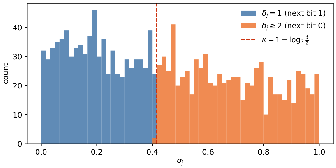
Figure 1. Histogram of the mantissas σ j for 3 2000 , split by the following gap. The two populations are exactly separated by the threshold κ = 2 log 2 3 (dashed line), as proved in Theorem 4.3.
Preprints 230437 g001
Figure 2. Density of ones in the binary expansion of 3 n , 1 n 5000 .
Preprints 230437 g002
Figure 3. Longest run of ones in 3 n versus the coin-tossing benchmark 2 log 2 n .
Preprints 230437 g003
Table 1. Binary representations of 3 n for n = 1 , , 10 .
n Binary representation
1 11
2 1001
3 11011
4 1010001
5 11110011
6 1011011001
7 100010001011
8 1100110100001
9 100110011100011
10 1110011010101001
Table 2. The truncated words λ 4 ( n ) = 3 n mod 64 and the mechanism eliminating each class in Proposition 5.17.
n mod 16 λ 4 ( n ) t = 5 h ( λ 4 ) eliminated by
0 1 4 Theorem 5.18 ( ν 2 ( n ) 4 )
1 3 3 p = 5
2 9 3 p = 5
3 27 1 parity (5.4)
4 17 3 — (survives)
5 51 1 p = 5
6 25 2 p = 5
7 11 2 — (survives)
8 33 3 p = 17
9 35 2 p = 5
10 41 2 p = 5
11 59 0 saturation
12 49 2 p = 17
13 19 2 p = 5
14 57 1 p = 5
15 43 1 p = 5
Table 3. Digit statistics of 3 n .
n L n h ( n ) h ( n ) / L n longest run of ones
10 16 9 0.5625 3
100 159 85 0.5346 5
500 793 406 0.5120 9
1000 1585 758 0.4782 7
2000 3170 1574 0.4965 10
5000 7925 3899 0.4920 13
Table 4. Density of ones: measured deviations from 1 2 against the spectral predictions ( K = 101 exponents per band).
n range M mean dev. s.d. 0.5 / M max|dev| / 0.5 2 log K / M
90–110 158 + 0.0015 0.0360 0.0398 0.0758 / 0.121
450–550 791 + 0.0028 0.0183 0.0178 0.0533 / 0.054
900–1100 1584 0.0009 0.0128 0.0126 0.0419 / 0.038
1900–2100 3169 + 0.0014 0.0080 0.0089 0.0280 / 0.027
3900–4100 6339 + 0.0002 0.0061 0.0063 0.0188 / 0.019
Table 5. Distribution of binary gaps in 3 2000 (1573 gaps) against two models.
d 1 2 3 4 5 6
empirical Pr ( δ = d ) , 3 2000 0.4997 0.2537 0.1208 0.0534 0.0394 0.0140
geometric 2 d 0.5000 0.2500 0.1250 0.0625 0.0313 0.0156
uniform- σ model | I d | 0.4150 0.2630 0.1520 0.0825 0.0431 0.0220
Disclaimer/Publisher’s Note: The statements, opinions and data contained in all publications are solely those of the individual author(s) and contributor(s) and not of MDPI and/or the editor(s). MDPI and/or the editor(s) disclaim responsibility for any injury to people or property resulting from any ideas, methods, instructions or products referred to in the content.
Copyright: This open access article is published under a Creative Commons CC BY 4.0 license, which permit the free download, distribution, and reuse, provided that the author and preprint are cited in any reuse.