Inverse Problem to Control the Coefficient of a Differential Equation in Time

Preprint

Article

Inverse Problem to Control the Coefficient of a Differential Equation in Time

This version is not peer-reviewed.

This version is not peer-reviewed.

Altmetrics

Downloads

183

Views

169

Comments

Submitted:

27 December 2023

Posted:

30 December 2023

Read the latest preprint version here

A peer-reviewed article of this preprint also exists.

Abstract

There are many problems based on solving non-autonomous differential equations of the form x¨(t)+ω2(t)x(t)=0, where x(t) represents the coordinate of a material point and ω is the angular frequency. The inverse problem involves finding the bounded coefficient ω. Continuity of the function ω(t) is not required. The trajectory x(t) is unknown, but the initial and final values of the phase variables are given. The variation principle of minimum time for the entire dynamic process allows for the determination of the optimal solution {x(t),ω(t)}. Thus, the inverse problem is an optimal control problem. No simplifying assumptions were made.

Keywords:

Subject:

Computer Science and Mathematics - Computational Mathematics

This preprints belongs to the Topic

Mathematical Modeling

Table 1. Notations to their definitions.

Notation	Description
$t, τ$	Time variables;
$x (t), y (t)$	Coordinate functions;
$\dot{x} (t)$	Velocity;
$\ddot{x} (t)$	Acceleration;
$ω (t)$	Control function;
$T, T_{1}, T_{2}, T_{o p t}$	Optimal time;
$\begin{matrix} A, A_{i}, C, B, \\ x (0), \dot{x} (0), x (T), \dot{x} (T) \end{matrix}$	Boundary conditions;
$t_{1}, t_{2}, t_{i}$	Switching points;
$ω_{0}$	Lower limited of the control function;
$ω_{i}$	Discrete values of $ω$ .

1. Introduction

The investigation of the equation

\ddot{x} (t) + ω^{2} (t) x (t) = 0,

(1)

where

ω (t)

is a given function, has a rich history and a wide range of applications. In the 19th century, Mathieu [1] studied solutions of this equation (1) for a special class of

ω (t) .

The research in this area began with the work of Magnus and Winkler on Hill’s equation [2]. Yakubovich and Starzhinskii [3] explored linear differential equations with periodic coefficients. This equation, in particular, describes the motion of a particle in a potential field, a problem that dates back to the work of K.M. Case [4] on singular coefficient. W.B. Case [5] examined the motion of a swing.

The inverse problem, where

ω (t)

is not given a priori and must be determined, is also field of interest but has been much less investigated.

Such problems arise, for example, in the theory of control of mechanical systems, when the goal is to find a control function that ensures the desired motion of a system [6].

The aim of this paper is to study the inverse problem the function

ω (t)

that guarantees the existence of a solution

x (t)

of the equation (1) satisfying the given final and initial conditions.

A more general problem related to equation (1) does not require smoothness of

ω (t)

and, in generally makes no simplifying assumptions about this function other than boundedness. The most natural formulation of the problem involves applying the variational principle to minimizing the total time of the process or some other objective function. It is also possible to give the problem a physical interpretation, considering parametric resonance [7], to find solutions where

x (t)

has an increasing amplitude, as well as conditions for damping oscillations.

The motivation of this work is to solve the inverse problem of the control with the coefficient

ω (t)

as a bang-bang control for the trajectories of equation (1). The function

ω (t)

can be applied in controllers for robotic systems [8]. Solutions to inverse control problems are generally non-classical. The smoothness of such solutions is violated at a finite number of isolated points. Therefore, between the switching points of the control function

ω (t)

the solution to the general problem

x (t)

(1) is smooth, allowing to cancel numerical methods to solve hard optimization problems. According to Pontryagin’s maximum principle [9]

ω (t)

imposes bounds, which simplifies the optimal control problem. Analytical methods are preferable to predict the

ω (t)

function, but exact solutions are rarely straightforward. It’s also worth noted that not all analytically solvable ill-posed problems can be easily solved numerically due to instability [10,11]. When additional constraints are imposed on the phase variables (for example,

| \dot{x (t)} | < const

), singular solutions to the

ω (t)

problem are possible [12]. In such cases, it is convenient to resort to numerical methods, which are widely available online in both open and private access, such as MATLAB, Python with SciPy, or Julia. The input data are assumed to be well-specified, so the main result of the work is to obtain nontrivial analytic solutions to the inverse control problem.

The complexity lies in the implicit connections between

ω (t), x (t),

and the total time

T,

and the need to satisfy all conditions simultaneously.

2. Preliminaries and problem formulation

An inverse problem of time optimal control for a second-order differential equation is considered. The objective is to determine the coefficient

ω (t)

of the differential equation, which is the boundary value problem:

\{\begin{matrix} \ddot{x} (t) = - ω^{2} (t) x (t), 0 < t < T; \\ x (0) = A > 0, \dot{x} (0) = 0; \\ x (T) = B \neq 0, \dot{x} (T) = 0, \end{matrix}

(2)

where

\{\begin{matrix} T \to i n f; \\ 0 \leq ω (t) \leq 1 or 0 < ω_{0} \leq ω (t) \leq 1, \end{matrix}

(3)

at the same time, the optimal process time T is unknown. Under these constraints, the function

ω (t)

can be found. The coefficient

ω (t)

is not smooth function indeed. The equation in the problem (2), (3) describes the motion of a material point with given boundary conditions. Initial conditions determine the position and speed of the point at the moment of time

t = 0 .

It is required in the shortest time T to move the point from the initial position to a given one, while the speed

\dot{x} (t)

at this moment should be equal to zero, and the entire trajectory should be a smooth function. The variational approach allows determining the controlling function

ω (t) .

Remark 2.1

The value of the constant A can be considered non-negative. If

A < 0,

then by replacing

y (t) = - x (t)

(due to the linearity of equation for

x (t)

), we arrive at the same equation for

y (t)

with the initial condition

y (0) > 0 .

Remark 2.2

The function

ω (t)

requires boundedness, but not continuity.

Remark 2.3

In real applications, the function

ω (t)

is typically non-negative. However, our approach can also find a solution for

ω (t)

when

\ddot{x} (t) - ω^{2} (t) x (t) = 0,

though this case is considered physically insignificant.

Remark 2.4

The condition of the initial and final velocities being zero is not a limitation. The proposed algorithm works in this scenario as well, but it leads to more cumbersome formulas

Remark 2.5

From a practical standpoint, the problem is not overdetermined, as technological processes in robotics aim for minimal time execution.

Remark 2.6

In problems (2) and (3), the stationary point

x = 0

of equation (1) is not investigated because the trajectory cannot converge to the point

x (T) = \dot{x} (T) = 0 .

Thus, the problem is reduced to two cases:

a.: If $0 \leq ω \leq 1,$ then the solution contains trigonometric and linear functions.
b.: The coefficient $ω (t)$ is limited and greater than zero ( $0 < ω_{0} \leq ω \leq 1$ ), the solution may oscillate, with the amplitude of oscillations increasing or decreasing over time.

In all these cases, the solutions for

x (t)

and

ω (t)

are explicit form. The number of switching points is limited. The problem is considered solved if all the switching points, trajectories, and the reachability set of are found.

3. Symmetry of the problem

Consider the following boundary problem:

\{\begin{matrix} \ddot{x} + ω^{2} (t) x = 0, 0 < t < T; \\ x (0) = A, \dot{x} (0) = 0; \\ x (T) = B, \dot{x} (T) = 0, \end{matrix}

(4)

where

A, B - const, A \cdot B \neq 0 .

Denoting

t = T - τ

leads to the same system:

\{\begin{matrix} \ddot{y} (τ) + ω^{2} (τ) y (τ) = 0, 0 < τ < T; \\ y (0) = B, \dot{y} (0) = 0; \\ y (T) = A, \dot{y} (T) = 0; \\ y (τ) = x (T - τ) . \end{matrix}

(5)

Thus, it is enough to consider the solution case (4) for all possible combinations of boundary conditions.

4. Analysis with $0 \leq ω \leq 1$

4.1. Different sign values at the boundary

Let’s again consider the system:

\{\begin{matrix} \ddot{x} + ω (t) x = 0, 0 < t < T; \\ x (0) = A > 0, \dot{x} (0) = 0; \\ x (T) = - B, \dot{x} (T) = 0, \end{matrix}

(6)

where

B = const > 0,

T \to i n f,

0 \leq ω (t) \leq 1, 0 \leq t \leq T,

x (t) \in C^{1} [0, T] .

There is a solution in the form (

ω = {0, 1}

x (t) = \{\begin{matrix} A cos (t), & 0 \leq t \leq t_{1}; \\ a t + b, & t_{1} \leq t \leq t_{2}; \\ B cos (t + Δ), & t_{2} \leq t \leq T . \end{matrix}

There is a system with continuity conditions for

x (t)

and

\dot{x} (t) :

\{\begin{matrix} A cos t_{1} = a t_{1} + b; \\ - A sin t_{1} = a; \\ B cos (t_{2} + Δ) = a t_{2} + b; \\ - B sin (t_{2} + Δ) = a; \\ T + Δ = π; \\ T \to i n f . \end{matrix}

(7)

Let’s express the auxiliary variables

a, b, t_{2}, Δ

through

t_{1} .

The solution (7) is sought analytically:

B^{2} = a^{2} + {(a t_{2} + b)}^{2} \Rightarrow a t_{2} + b = - \sqrt{B^{2} - a^{2}} (a t_{2} + b < 0 - under the axis) \Rightarrow

\{\begin{matrix} a = - A sin t_{1}; \\ b = A (cos t_{1} + t_{1} sin t_{1}); \\ t_{2} = \frac{1}{A sin t_{1}} (\sqrt{B^{2} - A^{2} {sin}^{2} t_{1}} + A (cos t_{1} + t_{1} sin t_{1})); \\ Δ = π - arcsin (\frac{A sin t_{1}}{B}) - t_{2}, \end{matrix}

resulting in the total non-optimal time of the process:

T = π - Δ (t_{1}) = arcsin (\frac{A sin t_{1}}{B}) + \frac{1}{A sin t_{1}} (\sqrt{B^{2} - A^{2} {sin}^{2} t_{1}} + A (cos t_{1} + t_{1} sin t_{1})) .

From the condition

T_{t_{1}}^{'} = 0 \Rightarrow t_{1} = \frac{π}{2} .

it turns out to be minimum total process time

T_{o p t} (B > A) = \frac{π}{2} + \frac{\sqrt{B^{2} - A^{2}}}{A} + arcsin (\frac{A}{B})

(8)

and the switching points

t_{1}, t_{2} :

\{\begin{matrix} t_{1} = \frac{π}{2}; \\ t_{2} = \frac{π}{2} + \frac{\sqrt{B^{2} - A^{2}}}{A} . \end{matrix}

The final solution is:

ω (t) = \{\begin{matrix} 1, & t \in [0, \frac{π}{2}) \cup [\frac{π}{2} + \frac{\sqrt{B^{2} - A^{2}}}{A}, T_{o p t}]; \\ 0, & t \in [\frac{π}{2}, \frac{π}{2} + \frac{\sqrt{B^{2} - A^{2}}}{A}), \end{matrix}

x (t) = \{\begin{matrix} A cos (t), & 0 \leq t \leq \frac{π}{2}; \\ - A (t - \frac{π}{2}), & \frac{π}{2} \leq t \leq \frac{π}{2} + \frac{\sqrt{B^{2} - A^{2}}}{A}; \\ - B cos (t - T_{o p t}), & \frac{π}{2} + \frac{\sqrt{B^{2} - A^{2}}}{A} \leq t \leq T_{o p t} . \end{matrix}

It is noted that this solution is optimal. If

B < A,

a similar analysis of the system (6) leads to the formulas:

T_{o p t} (B < A) = \frac{π}{2} + \frac{\sqrt{A^{2} - B^{2}}}{B} + arcsin (\frac{B}{A}) .

(9)

The final solution is:

ω (t) = \{\begin{matrix} 1, & t \in [0, arcsin (\frac{B}{A})) \cup [\frac{\sqrt{A^{2} - B^{2}}}{B} + arcsin (\frac{B}{A}), T_{o p t}); \\ 0, & t \in [arcsin (\frac{B}{A}), \frac{\sqrt{A^{2} - B^{2}}}{B} + arcsin (\frac{B}{A})), \end{matrix}

x (t) = \{\begin{matrix} A cos t, & t \in [0, arcsin (\frac{B}{A})]; \\ B (\frac{\sqrt{A^{2} - B^{2}}}{B} + arcsin (\frac{B}{A}) - t), & t \in [arcsin (\frac{B}{A}), \frac{\sqrt{A^{2} - B^{2}}}{B} + arcsin (\frac{B}{A})]; \\ - B cos (t - T_{o p t}), & t \in [\frac{\sqrt{A^{2} - B^{2}}}{B} + arcsin (\frac{B}{A}), T_{o p t}] . \end{matrix}

All possible solutions can be found on Figure 1.

4.2. Proof of optimality

It is easy to show that using value

ω \notin {0, 1}

leads to a non-optimal solution.

The system for the general case looks like:

x (t) = \{\begin{matrix} A cos (α t), & 0 \leq t \leq t_{1}; \\ a t + b, & t_{1} \leq t \leq t_{2}; \\ B cos (α t), & t_{2} \leq t \leq T . \end{matrix}

After some algebra the solution leads to

T (B > A) = t_{1} + \frac{1}{β} arcsin (\frac{A α}{B β} sin (t_{1})) - (\frac{1}{A} \sqrt{B^{2} - \frac{A^{2} α^{2}}{β^{2}} {sin}^{2} (t_{1})} - cos (t_{1})) \frac{1}{α sin (t_{1})} .

To get the minimal time

T_{m i n}

it is needed to solve the equation

T_{t_{1}}^{'} = 0 .

The final parameters are

α = β = 1, t_{1} = \frac{π}{2} .

The same calculation can be done for the case

T (B < A) .

4.3. Identical sign values at the boundary

Let’s now consider the case when the values on the boundaries are of the same sign:

\{\begin{matrix} \ddot{x} + ω (t) x = 0, 0 \leq t \leq T; \\ x (0) = A, \dot{x} (0) = 0; \\ x (T) = B, \dot{x} (T) = 0, \end{matrix}

(10)

where

A, B = const, T \to i n f, 0 \leq ω (t) \leq 1, x (t) \in C^{1} [0, T] .

Also, let’s assume

0 < A < B .

It should be noted that in this case the solution is non-monotonic, i.e. the coordinate undergoes one full oscillation.

Indeed,

1.: For any $ω (t) \in [0, 1]$ there is exist $t_{0}^{*}$ such that: $x (t_{0}^{*}) = 0, \dot{x} (t_{0}^{*}) < 0, x (t) > 0, t \in (0, t_{0}^{*}) .$
2.: For any $ω (t) \in [0, 1]$ there is exist $t_{1}^{*}$ such that: $x (t_{1}^{*}) < 0, \dot{x} (t_{1}^{*}) = 0, x (t) < 0, t \in (t_{0}^{*}, t_{1}^{*}) .$

Moreover,

1.: For any $ω (t) \in [0, 1]$ there is exist $t_{2}^{*}$ such that: $x (t_{2}^{*}) = 0, \dot{x} (t_{2}^{*}) > 0, x (t) < 0, t \in (t_{1}^{*}, t_{2}^{*}) .$
2.: For any $ω (t) \in [0, 1]$ there is exist $t_{3}^{*}$ such that: $x (t_{3}^{*}) > 0, \dot{x} (t_{3}^{*}) = 0, x (t) > 0, t \in (t_{2}^{*}, t_{3}^{*}) .$

These propositions lead to the construction of a solution.

Clearly, if we consider the points

t_{0}^{*}, t_{1}^{*}, t_{2}^{*}, t_{3}^{*},

and the previously constructed solution

x (t), t \in (0, t_{3}^{*})

with the described properties, and set

T = t_{3}^{*},

then the constructed solution will be optimal.

In fact, let’s consider the point

t_{1}^{*},

where

x (t_{1}^{*}) < 0, \dot{x} (t_{1}^{*}) = 0 .

An optimal solution on the interval

[0, t_{1}^{*}]

can then be constructed. This solution precisely addresses the problem where values of different signs are accepted at the boundaries, as discussed earlier..

Similarly, by solving the problem for the interval

[t_{1}^{*}, T],

we obtain the optimal part of the solution.

In other words, there are lower estimates for

t_{1}^{*}

and

T - t_{1}^{*} .

Since the boundary conditions of the problems at the point

t = t_{1}^{*}

are identical, the obtained solution is defined on

[0, T]

and belong to the class

C^{1} [0, T] .

However, to solve each of the problems separately, it is necessary to know the value of

x (t_{1}^{*}) < 0 .

In fact, determining this value is essential because the analytical formulas for the length of the interval and the solutions for each part have already been obtained (see equations (8), (9)).

Thus, the problem is formalized, which will be equivalent to the original one (see equation (10)).

This problem is divided into two parts: for

t \in [0, T_{1}]

and for

t \in [T_{1}, T_{2}] .

Ultimately, it is necessary to minimize

T_{1} + T_{2} :

T_{1} = \frac{π}{2} + \frac{\sqrt{A_{1}^{2} - A^{2}}}{A} + arcsin (\frac{A}{A_{1}}), T_{2} = \frac{π}{2} + \frac{\sqrt{B^{2} - A_{1}^{2}}}{A_{1}} + arcsin (\frac{A_{1}}{B}),

here

A_{1}

is a parameter through which the optimal curve must pass.

\begin{matrix} \frac{d (T_{1} + T_{2})}{d A_{1}} = \frac{A_{1}}{A} \frac{1}{\sqrt{A_{1}^{2} - A^{2}}} - \frac{A}{A_{1}^{2}} \frac{1}{\sqrt{1 - A^{2} / A_{1}^{2}}} + \\ + \frac{- A_{1}}{A_{1} \sqrt{B^{2} - A_{1}^{2}}} - \frac{\sqrt{B^{2} - A_{1}^{2}}}{A_{1}^{2}} + \frac{1}{B \sqrt{1 - A_{1}^{2} / B^{2}}} = 0 \\ \Rightarrow A_{1} = \sqrt{A B} \Rightarrow T_{1} = T_{2} = \frac{π}{2} + \frac{\sqrt{B - A}}{\sqrt{A}} + arcsin (\sqrt{\frac{A}{B}}), \end{matrix}

optimal time of this process:

T_{o p t} (B > A) = π + 2 \sqrt{\frac{B}{A} - 1} + 2 arcsin (\sqrt{\frac{A}{B}}) .

The final solution is:

ω (t) = \{\begin{matrix} 1, & t \in (0, \frac{π}{2}) \cup [t_{1}, t_{2}) \cup [t_{3}, T_{o p t}); \\ 0, & t \in [\frac{π}{2}, t_{1}) \cup [t_{2}, t_{3}), \end{matrix}

x (t) = \{\begin{matrix} A cos t, & t \in [0, \frac{π}{2}]; \\ A (\frac{π}{2} - t), & t \in [\frac{π}{2}, t_{1}]; \\ - \sqrt{A B} cos (t - (t_{2} - \frac{π}{2})), & t \in [t_{1}, t_{2}]; \\ \sqrt{A B} (t - t_{2}), & t \in [t_{2}, t_{3}]; \\ B cos (t - T_{o p t}), & t \in [t_{3}, T_{o p t}], \end{matrix}

where

\{\begin{matrix} t_{1} = \frac{π}{2} + \sqrt{\frac{B}{A} - 1}, \\ t_{2} = π + \sqrt{\frac{B}{A} - 1} + arcsin (\sqrt{\frac{A}{B}}), \\ t_{3} = π + 2 \sqrt{\frac{B}{A} - 1} + arcsin (\sqrt{\frac{A}{B}}) . \end{matrix}

T_{o p t} (B < A) = π + 2 \sqrt{\frac{A}{B} - 1} + 2 arcsin (\sqrt{\frac{B}{A}}),

ω (t) = \{\begin{matrix} 1, & t \in (0, t_{1}) \cup [t_{2}, t_{3}) \cup [t_{4}, T_{o p t}); \\ 0, & t \in [t_{1}, t_{2}) \cup [t_{3}, t_{4}), \end{matrix}

x (t) = \{\begin{matrix} A cos t, & t \in [0, t_{1}]; \\ \sqrt{A B} (t_{2} - t), & t \in [t_{1}, t_{2}]; \\ \sqrt{A B} cos (t - (t_{2} - \frac{π}{2})), & t \in [t_{2}, t_{3}]; \\ B (t - t_{4}), & t \in [t_{3}, t_{4}]; \\ B cos (t - T_{o p t}), & t \in [t_{4}, T_{o p t}], \end{matrix}

where

\{\begin{matrix} t_{1} = arcsin (\sqrt{\frac{B}{A}}); \\ t_{2} = arcsin (\sqrt{\frac{B}{A}}) + \sqrt{\frac{A}{B} - 1}; \\ t_{3} = \frac{π}{2} + \sqrt{\frac{A}{B} - 1} + 2 arcsin (\sqrt{\frac{B}{A}}); \\ t_{4} = \frac{π}{2} + 2 \sqrt{\frac{A}{B} - 1} + 2 arcsin (\sqrt{\frac{B}{A}}) . \end{matrix}

The set of reachability is constructed for two cases when the boundary values of the coordinate

x (0)

and

x (T)

are of different signs - Figure 1 and the same sing - Figure 2. It should be noted that the maximum number of switches in the case of

0 \leq ω (t) \leq 1

is equal to

4 .

The simple solution

x (t) = A cos t

with

ω = 1

of (4) is interface curve of the two different regimes:

B > A

and

B < A

of system (4).

Similarly, one can consider the case of separation from zero, i.e.,

0 < ω_{0} \leq ω (t) \leq 1 .

5. Problem with $ω > 0$

5.1. Construction of an analytical solution when $ω > 0$

Let’s set the problem of determining the optimal process for achieving the final value of the coordinate

x (T) = B .

Let

ω (t) \in [ω_{0}, 1],

where

ω_{0} > 0 .

| x (T) | > A,

in this case, parametric resonance occurs [7], when the final value is obtained after a large number of switches. In this case, the amplitude of oscillations

x (t)

increases with the growth of t under the condition of minimum total process time.

| x (T) | < A

, in this case, the effect of damping occurs. In this case, the amplitude of oscillations

x (t)

decays with the growth of

t .

Oscillations with

| x (T) | \neq A

occur with a changing amplitude.

Let’s introduce a division of the segment

[0, T]

into intervals

[t_{i}, t_{i + 1}], i = 0, 1, \dots, (N + 1), t_{0} = 0, t_{N + 2} = T .

Then

ω (t)

is represented as a piecewise-constant function, which allows finding an analytical solution, as

ω (t)

only takes two values:

ω (t) = {ω_{0}, 1}

according to Pontryagin’s maximum principle [9].

Consider the coordinate function

x (t) \in C^{1} [0, T] : \{\begin{matrix} x (0) = A; \\ \dot{x} (0) = \dot{x} (T) = 0, \end{matrix}

of the following form:

x (t) = \{\begin{matrix} A cos (α t), & 0 \leq t \leq t_{1}; \\ A_{1} cos (ω_{1} t + δ_{1}), & t_{1} \leq t \leq t_{2}; \\ \dots & \dots \\ A_{i} cos (ω_{i} t + δ_{i}), & t_{i} \leq t \leq t_{i + 1}; \\ \dots & \dots \\ A_{N} cos (ω_{N} t + δ_{N}), & t_{N} \leq t \leq t_{N + 1}; \\ B cos (β t + Δ), & t_{N + 1} \leq t \leq T, \end{matrix}

(11)

where

t_{i}, i = 1, 2, \dots, (N + 1)

are the points of pairing,

B \in R {0}

is terminal value. The task of determining

ω (t)

is reduced to finding the values

{ω_{i}, t_{i}, A_{i}, δ_{i}, α, β, Δ} .

Note that the intervals

[t_{i}, t_{i + 1}]

can be of unequal length.

Based on this, clarify the main goal: from all such functions

x (t),

one should choose such that the total time of the process T is minimal.

The variational setting should be supplemented with the conditions of differentiability of the trajectory

x (t)

and the continuity of the velocity

\dot{x} (t)

at the points of pairing.

Note that the maximum principle is not fulfilled for

ω (t)

in the presence of some constraints.

Thus, calculations lead to a recursive relation, determined by formulas (11) with

N = 0, 1, \dots, M .

The number of switches is defined unambiguously, but if a smaller number of switches is set, then the boundary conditions (2), are not fulfilled; if more, then part of the time intervals degenerates into points. For the verification of analytical solutions, a numerical calculation was performed taking into account formulas (11) with 1000 possible switches, and the calculations confirmed the analytical solution.

As a result, the task can be divided into a family of separate boundary tasks, where the boundary conditions are recurrently determined by the conditions of pairing:

A_{i} = \sqrt{A_{i - 1} A_{i + 1}}

A_{0} = A, A_{N + 1} = B .

A_{i} = {(\sqrt[N]{A B})}^{i}

The proof of optimality is based on the dependency of the solution on the initial and terminal conditions on each full oscillation and will be given below.

Thus, the solution

x (t)

represents a smooth curve. The number of oscillations depends on the position of the final point

x (T)

inside reachability set.

1.

x (T) < 0,

then the following cases of the optimal process are possible:

a): $x (T) = - A ω_{0}^{- 1}$ or $x (T) = - A ω_{0}$ ;
b): $x (T) : - A ω_{0}^{- 1} < x (T) < - A ω_{0}$ ;
c): If $x (T) \notin [- A ω_{0}^{- 1}, - A ω_{0}],$ then the solution oscillates with a number of switches.

2.

x (T) > 0, x (T) \neq A,

then

a): $x (T) = A ω_{0}^{- 2}$ or $x (T) = A ω_{0}^{2}$ ;
b): $x (T) \in [A ω_{0}^{2}, A ω_{0}^{- 2}]$ ;
c): If $x (T) \notin [A ω_{0}^{2}, A ω_{0}^{- 2}],$ then the solution oscillates with a number of switches.

One switch.

For the final point

x (T) < 0,

let’s consider the case with one switching point. We obtain that the function

x (t)

consists of two cosines:

x (t) = \{\begin{matrix} A cos (α t), & 0 \leq t \leq t_{1}; \\ B cos (β t + Δ), & t_{1} < t \leq T, A, B > 0 . \end{matrix}

Let’s write the conditions of continuity and the existence of the derivative at the point

t_{1} \in [0, T],

i.e.

\{\begin{matrix} A cos (α t_{1}) = B cos (β t_{1} + Δ); \\ A α sin (α t_{1}) = B β sin (β t_{1} + Δ) . \end{matrix}

(12)

It leads to

B = A \sqrt{1 + {sin}^{2} (α t_{1}) ({(\frac{α}{β})}^{2} - 1)}

(13)

t_{1} = \frac{1}{α} arcsin \sqrt{\frac{(B^{2} - A^{2}) β^{2}}{A^{2} (α^{2} - β^{2})}} if A α \geq B β,

(14)

α, β \in [ω_{0}, 1], 0 \leq {sin}^{2} (α t_{1}) \leq 1 \Rightarrow

A ω_{0} \leq B \leq A ω_{0}^{- 1} .

Let’s consider characteristic cases:

If $B = A ω_{0},$ then $\{\begin{matrix} {sin}^{2} α t_{1} = 1; \\ α = ω_{0}, β = 1, \end{matrix}$ the solution is: $α = ω_{0}, β = 1, t_{1} = \frac{π}{2 ω_{0}},$ then the function $x (t)$ is uniquely determined $T = \frac{π}{2} (1 + ω_{0}^{- 1}) .$
If $B = \frac{A}{ω_{0}},$ then discussing similarly to the previous case, we obtain that the function $x (t)$ is determined similarly: $α = 1, β = ω_{0}, t_{1} = \frac{π}{2}, T_{o p t} = \frac{π}{2} (1 + ω_{0}^{- 1}) .$
If $B = A,$ then the function $x (t)$ is determined as follows:

$[\begin{matrix} t_{1} = π k, k = 0, 1, \forall α, β; \\ α = β, \forall t_{1} \end{matrix} \Rightarrow [\begin{matrix} t_{1} = 0 and Δ = 0 \Rightarrow x (t) = A cos (β t); \\ t_{1} = π \Rightarrow x (t) = A cos (α t); \\ α = β \Rightarrow x (t) = A cos (α t) \end{matrix}$

In this case, the function will be equal to $A \cdot cos (α t), α \in [ω_{0}, 1], T = \frac{π}{α} .$ Taking into account the minimum $T,$ we get that $α = 1$ and $x (t)$ is determined unambiguously.

6. Construction of the optimal solution

As was mentioned earlier - the optimal solution from A to

(- B),

where

B \in [A ω_{0}, \frac{A}{ω_{0}}],

will consist of one, two, or three cosines.

Let’s consider the function

x (t) = \{\begin{matrix} A cos (ω_{1} t), & 0 \leq t \leq t_{1}; \\ C cos (ω_{2} t + δ), & t_{1} \leq t \leq t_{2}; \\ B cos (ω_{3} t + Δ), & t_{2} \leq t \leq T . \end{matrix}

Proposition: let

ω_{1} = ω_{3} = 1, ω_{2} = ω_{0} > 0

, B is known, then

x (t) = \{\begin{matrix} A cos (t), & 0 \leq t \leq t_{1}; \\ C cos (ω_{0} t + δ), & t_{1} \leq t \leq t_{2}; \\ B cos (t + Δ), & t_{2} \leq t \leq T . \end{matrix}

According to the maximum principle [9] two values of

ω (t)

are admissible as well.

Construct an analytical optimal solution and prove that it is optimal.

Let’s write the continuity conditions and the existence of the derivative at the points

t_{1}, t_{2} :

\{\begin{matrix} A cos (t_{1}) = C cos (ω_{0} t_{1} + δ); \\ - A sin (t_{1}) = - C ω_{0} sin (ω_{0} t_{1} + δ); \\ C cos (ω_{0} t_{2} + δ) = B cos (t_{2} + Δ); \\ - C ω_{0} sin (ω_{0} t_{2} + δ) = - B sin (t_{2} + Δ) . \end{matrix}

Let’s express the unknowns through

t_{1} .

Let’s write the conditions of continuity and the existence of the derivative at the point

t_{1},

i.e.

\{\begin{matrix} A cos (t_{1}) = C cos (ω_{0} t_{1} + δ) \\ A sin (t_{1}) = C ω_{0} sin (ω_{0} t_{1} + δ) . \end{matrix}

(15)

Using the basic trigonometric identity, we have (we divide the second equation by

ω_{0},

raise each equation to the second power, and sum them up):

C = A \sqrt{1 + {sin}^{2} (t_{1}) ({(\frac{1}{ω_{0}})}^{2} - 1)},

(16)

From the first equation, let’s express

δ :

δ (t_{1}) = arccos (\frac{A cos t_{1}}{C}) - ω_{0} t_{1}

Let’s write the conditions of continuity and the existence of the derivative at the point

t_{2},

i.e.

\{\begin{matrix} C cos (ω_{0} t_{2} + δ) = B cos (t_{2} + Δ) \\ C ω_{0} sin (ω_{0} t_{2} + δ) = B sin (t_{2} + Δ) . \end{matrix}

(17)

Using the basic trigonometric identity, we have (raise each equation to the second power and sum them up):

C^{2} ({cos}^{2} (ω_{0} t_{2} + δ) + ω_{0}^{2} {sin}^{2} (ω_{0} t_{2} + δ)) = B^{2},

(18)

\begin{matrix} C^{2} (ω_{0}^{2} + (1 - ω_{0}^{2}) {cos}^{2} (ω_{0} t_{2} + δ)) = B^{2} \Rightarrow (1 - ω_{0}^{2}) {cos}^{2} (ω_{0} t_{2} + δ) = \frac{B^{2}}{C^{2}} - ω_{0}^{2} \Rightarrow \\ {cos}^{2} (ω_{0} t_{2} + δ) = \frac{B^{2} - C^{2} ω_{0}^{2}}{C^{2} (1 - ω_{0}^{2})} \Rightarrow t_{2} = \frac{1}{ω_{0}} (π - arccos \sqrt{\frac{C^{2} - B^{2} ω_{0}^{2}}{B^{2} (1 - ω_{0}^{2})}} - δ) . \end{matrix}

(19)

Δ (t_{1}) = arccos (\frac{C cos (ω_{0} t_{2} + δ)}{B}) - t_{2}

It turns out that all unknown variables are expressed through

t_{1} :

\{\begin{matrix} C = A \sqrt{1 + {sin}^{2} (t_{1}) ({(\frac{1}{ω_{0}})}^{2} - 1)}; \\ δ (t_{1}) = arccos (\frac{A cos t_{1}}{C}) - ω_{0} t_{1}; \\ t_{2} = \frac{1}{ω_{0}} (π - arccos \sqrt{\frac{B^{2} - C^{2} ω_{0}^{2}}{C^{2} (1 - ω_{0}^{2})}} - δ); \\ Δ (t_{1}) = arccos (\frac{C cos (ω_{0} t_{2} + δ)}{B}) - t_{2}; \\ T (t_{1}) = π - arccos (\frac{C cos (ω_{0} t_{2} + δ)}{B}) + t_{2} . \end{matrix}

(20)

After some algebra the system (20) gives us the solution.

The optimal time T is found from the condition

\frac{d T (t_{1})}{d t_{1}} = 0

The solution:

\begin{matrix} t_{1} = \frac{π}{2}, δ = (1 - ω_{0}) \frac{π}{2}, C = \frac{A}{ω_{0}}; \\ t_{2} = \frac{1}{ω_{0}} (\frac{π}{2} (1 + ω_{0}) - arccos (ω_{0} \sqrt{\frac{B^{2} - A^{2}}{A^{2} (1 - ω_{0}^{2})}})); \\ Δ = arccos (\frac{A cos (ω_{0} t_{2} + δ)}{ω_{0} B}) - t_{2}; \\ T (B) = π - Δ . \end{matrix}

These considerations will help us come up with a solution.

7. Proof of optimality and final solution

Let’s consider the following case

A > 0 \overset{T_{1}}{\to} (- C) \overset{T_{2}}{\to} B,

where

B \in [A ω_{0}^{2} A / ω_{0}^{2}],

T = T_{1} + T_{2} :

A \overset{T_{1}}{\to} (- C) : x (t) = \{\begin{matrix} \ddot{x} + ω^{2} (t) x = 0, 0 < t < T_{1}; \\ x (0) = A, \dot{x} (0) = 0; \\ x (T_{1}) = - C, \dot{x} (T_{1}) = 0, \end{matrix}

(21)

and

(- C) \overset{T_{2}}{\to} B : x (t) = \{\begin{matrix} \ddot{x} + ω^{2} (t) x = 0, T_{1} < t < T; \\ x (T_{1}) = - C, \dot{x} (T_{1}) = 0; \\ x (T) = B, \dot{x} (T) = 0, \end{matrix}

(22)

For the problems (21), (22) the solution for the optimal time

T_{1}

and

T_{2} :

T_{1} = \frac{π}{2} (1 + \frac{1}{ω_{0}}) + arccos (\frac{1}{C} \sqrt{\frac{C^{2} - A^{2}}{1 - ω_{0}^{2}}}) - \frac{1}{ω_{0}} arccos (\frac{ω_{0}}{A} \sqrt{\frac{C^{2} - A^{2}}{1 - ω_{0}^{2}}});

(23)

T_{2} = \frac{π}{2} (1 + \frac{1}{ω_{0}}) + arccos (\frac{1}{B} \sqrt{\frac{B^{2} - C^{2}}{1 - ω_{0}^{2}}}) - \frac{1}{ω_{0}} arccos (\frac{ω_{0}}{C} \sqrt{\frac{B^{2} - C^{2}}{1 - ω_{0}^{2}}}) .

(24)

Let’s study first derivative:

\frac{d (T_{1} + T_{2})}{d C} = 0 \Rightarrow C = \sqrt{A B} - minimum value \Rightarrow T_{1} = T_{2},

where

\begin{matrix} \frac{π}{2}, \frac{1}{ω_{0}} (\frac{π}{2} (1 + ω_{0}) - arccos (\frac{ω_{0}}{A} \sqrt{\frac{C^{2} - A^{2}}{A^{2} (1 - ω_{0}^{2})}})) - \\ switching points t_{1}, t_{2} Figure a); \end{matrix}

(25)

\begin{matrix} T_{1} + \frac{π}{2}, T_{1} + \frac{1}{ω_{0}} (\frac{π}{2} (1 + ω_{0}) - arccos (\frac{ω_{0}}{C} \sqrt{\frac{B^{2} - C^{2}}{C^{2} (1 - ω_{0}^{2})}})) - \\ switching points for t \in [t_{1}, T] . \end{matrix}

(26)

For the case

b)

on Figure 3 solution is

T^{★} = T_{1}^{★} + T_{2}^{★}

\begin{matrix} T_{1}^{★} = \frac{π}{2} (1 + ω_{0}) - \frac{1}{ω_{0}} arccos (\frac{1}{C} \sqrt{\frac{C^{2} - A^{2}}{1 - ω_{0}^{2}}}) + arccos (\frac{ω_{0}}{A} \sqrt{\frac{C^{2} - A^{2}}{1 - ω_{0}^{2}}}); \\ T_{2}^{★} = \frac{π}{2} (1 + ω_{0}) - \frac{1}{ω_{0}} arccos (\frac{1}{B} \sqrt{\frac{B^{2} - C^{2}}{1 - ω_{0}^{2}}}) + arccos (\frac{ω_{0}}{C} \sqrt{\frac{B^{2} - C^{2}}{1 - ω_{0}^{2}}}) . \end{matrix}

At the point

C = \sqrt{A B}

, the maximum of

T^{★}

is reached, but this time is not optimal.

From the obtained formulas, it follows that the solution to the original problem is unique, as it is constructed in explicit form.

Remark.

The issue of optimality can be solved through the maximum principle [9]. However it’s proved by direct classical analysis.

Thus, the complete solution of the problem of determining the optimal process consists in finding amplitudes according to the formulas:

A_{i} = \sqrt{A_{i - 1} A_{i + 1}},

A_{0} = A, A_{N} = B

and the time

T = \sum_{i = 1}^{N} T_{i},

where

T_{i}

- is the time of one full oscillation. The choice of sign for

A_{i}

is determined from the reachability set.

8. General case

Write the condition of pairing at an arbitrary point

t_{i} :

\{\begin{matrix} A_{i} cos (ω_{i} t_{i} + δ_{i}) = A_{i + 1} cos (ω_{i + 1} t_{i} + δ_{i + 1}); \\ A_{i} ω_{i} sin (ω_{i} t_{i} + δ_{i}) = A_{i + 1} ω_{i + 1} sin (ω_{i + 1} t_{i} + δ_{i + 1}), \end{matrix}

(27)

where

A_{i}, ω_{i}, δ_{i}

are known (they are determined at the previous point of pairing).

Note that if

ω_{i} t_{i} + δ_{i} = ω_{i + 1} t_{i} + δ_{i + 1} = π k, k \in N,

then

A_{i} = A_{i + 1},

and

ω_{i + 1}, δ_{i + 1}

are paired by the equation

ω_{i + 1} t_{i} + δ_{i + 1} = π k,

in which any

ω_{i + 1} \in [ω_{0}, 1]

can be taken.

ω_{i} t_{i} + δ_{i} = ω_{i + 1} t_{i} + δ_{i + 1} = \frac{π}{2} + π k, k \in N_{0},

then

A_{i} ω_{i} = A_{i + 1} ω_{i + 1},

and

δ_{i + 1}

is determined from the equation

ω_{i + 1} t_{i} + δ_{i + 1} = \frac{π}{2} + π k .

Let’s consider the function

x (t)

for an arbitrary

N > 0 .

Writing the conditions of continuity and the existence of the derivative at the points

t_{i}, i = 1, 2, \dots, N

we have:

B = A \sqrt{1 + {sin}^{2} (α t_{1}) ({(\frac{α}{ω_{1}})}^{2} - 1)} \sqrt{1 + {sin}^{2} (ω_{1} t_{2} + δ_{1}) ({(\frac{ω_{1}}{ω_{2}})}^{2} - 1)} \cdot \dots

\dots \cdot \sqrt{1 + {sin}^{2} (ω_{N} t_{N + 1} + δ_{N}) ({(\frac{ω_{N}}{β})}^{2} - 1)} .

Hence, it leads that

A ω_{0}^{N} \leq B \leq \frac{A}{ω_{0}^{N}}

In conclusion, we get that the set

D_{ω_{0}} = [A ω_{0}^{N}, \frac{A}{ω_{0}^{N}}]

is the set of controllability (reachability).

9. Construction of the set of reachability

Let N be the number of zeros of the function

x (t)

on the set

(0, T],

and

A = x (0),

ω_{0} \neq 0 .

Consider the following family of sets for negative final values:

\begin{matrix} A_{-}^{1} = [- A ω_{0}, \frac{- A}{ω_{0}}], A_{-}^{N} = (\frac{- A}{ω_{0}^{N - 2}}, \frac{- A}{ω_{0}^{N}}], \\ B_{-}^{N} = (- A ω_{0}^{N}, - A ω_{0}^{N - 2}], N = 2 k + 1, k \in N . \end{matrix}

For positive final values:

\begin{matrix} A_{+}^{2} = [A ω_{0}^{2}, \frac{A}{ω_{0}^{2}}], A_{+}^{N} = (\frac{A}{ω_{0}^{N - 2}}, \frac{A}{ω_{0}^{N}}], \\ B_{+}^{N} = (A ω_{0}^{N}, A ω_{0}^{N - 2}], N = 2 k, k \in N, k \in N . \end{matrix}

These sets enable the determination of the optimal process time corresponding to the specific trajectory.

Let’s outline the process for determining the optimal trajectory:

1.: Determine the optimal time curve that $x (T)$ belongs to.
2.: Choose a trajectory that converges to the terminal point; this trajectory will be optimal (see Figure 4)
3.: Construct the analytical solution within a single oscillation and extend it to the terminal point using Eq. (23),(24) and Eq. (25),(26).

The boundary of the intervals are connected by convex functions

T (B) .

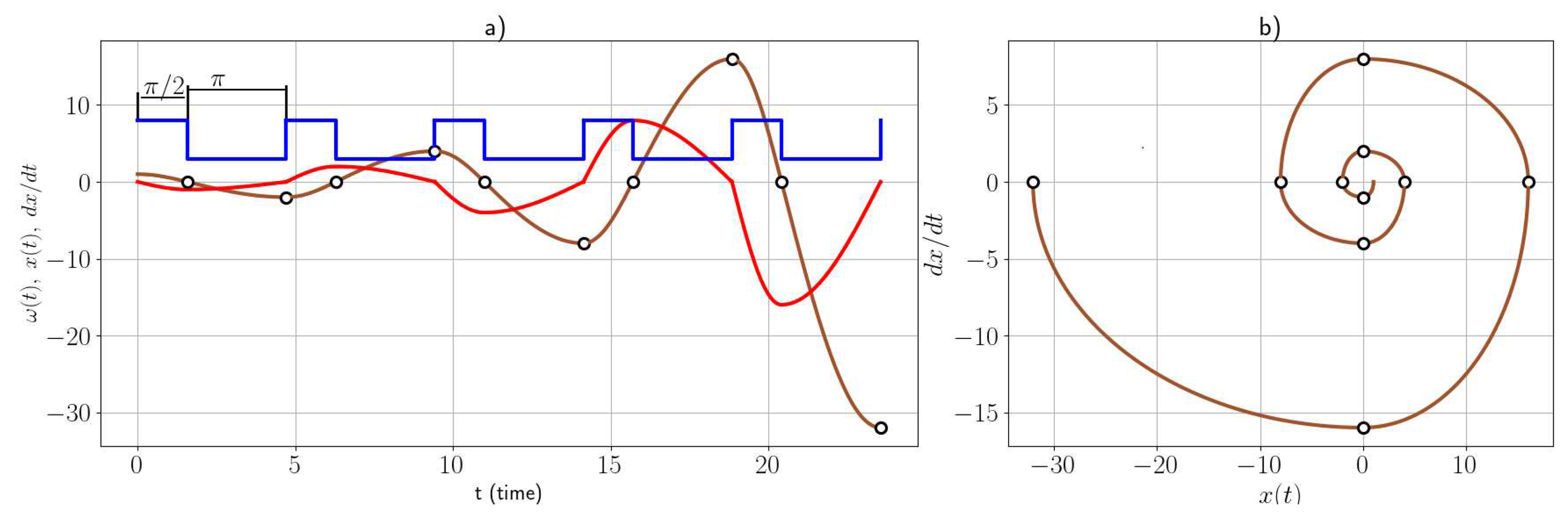
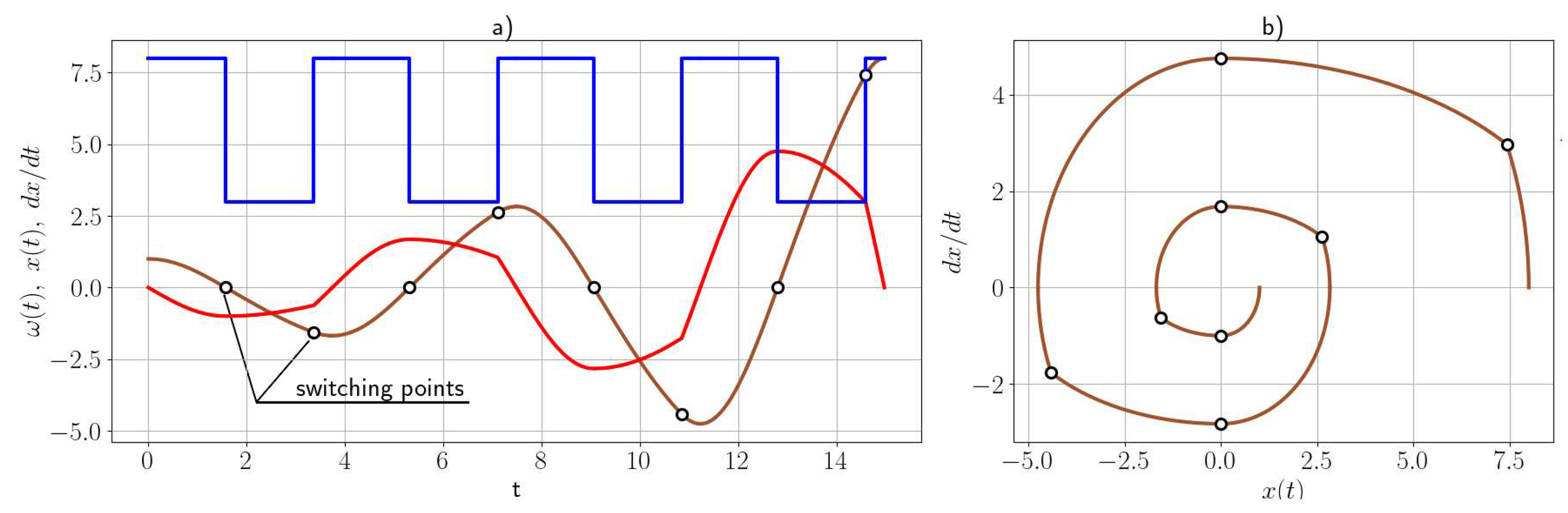
Figure 6. A time optimal trajectory of oscillations

a)

and the phase portrait

b)

with switching points

x (0) = 1, \dot{x} (0) = 0, x (T) = - 32, \dot{x} (T) = 0, 0.5 \leq ω (t) \leq 1, T \approx 23.56 .

The oscillations follow the boundary of the reachability set.

Figure 6. A time optimal trajectory of oscillations

a)

and the phase portrait

b)

with switching points

x (0) = 1, \dot{x} (0) = 0, x (T) = - 32, \dot{x} (T) = 0, 0.5 \leq ω (t) \leq 1, T \approx 23.56 .

The oscillations follow the boundary of the reachability set.

10. Conclusions and outlook

In this paper, we address the multiparameter problem of optimally controlling the coefficients of a linear differential equation in the shortest possible time. The instability of the inverse control problem leads to difficulties in obtaining a reliable solution by numerical method. Therefore, the solution is constructed analytically and verified through direct modeling, using recurrent formulas for each trajectory segment while ensuring smoothness.

The following results were obtained:

Constraints on the parameters under which nontrivial solutions occur were established.
Points were identified where the coefficients of the equation can be switched, for arbitrary input parameters, to achieve an optimal solution.
The reachability set was constructed for the conditions $0 \leq ω (t) \leq 1$ and $0 < ω_{0} \leq ω (t) \leq 1 .$

In the problem under consideration, the trend

μ \dot{x},

where

μ > 0

, was not included; this aspect will be the subject of research in the subsequent article.

11. Declaration of competing interest

The authors declare that they have no known competing financial interests of personal relationships that could have appeared to influence the work reported in this paper.

References

E. Mathieu. Course de physique mathematique. Publisher: Paris, France, 1973.
S. Magnus, W. Winkler. Hill’s equation. Publisher: Dover Publications, January 26, 2004.
V.A. Yakubovich, V.M. Starzhinskii. Linear differential equations with periodic coefficients, Wiley, 1975.
K. M. Case. Singular potentials. Physical Review, 80(5), 1950; 797. [CrossRef]
W. B. Case. The pumping of a swing from the standing position. American Journal of Physics. 64 (3), 1996, pp.215-220. [CrossRef]
G. Yakubu, P. Olejnik, J. Awrejcewicz. On the modeling and simulation of variable - length pendulum. Archives of computational methods in engineering, 29:, 2022, 2397-2415. [CrossRef]
L. Hatvani. On the parametrically excited pendulum equation with a step function coefficient. International journal of non-linear mechanics, 77, 2015, pp.172-182. [CrossRef]
Q. Luo, C. Chevallereau, Y. Aoustin. Walking Stability of a Variable Length. Inverted Pendulum Controlled with Virtual Constraints International journal of humanoid robotics, 2019, pp.1950040. [CrossRef]
L.S. Pontryagin. The mathematical theory of optimal processes., 1st ed.; Publisher: London, UK, 1987; p. 360. [CrossRef]
S. Walczak. Well-posed and ill-posed optimal control problems. Journal of optimization theory and applications, vol. 109, No.1, 04.2001, 169–185. [CrossRef]
F. Po¨rner. Regularization methods for ill-posed optimal control problems. Doctoral thesis. Wu¨rzburg University Press; 2018. [CrossRef]
J. Flaherty, R. O’Malley. On the computation of singular controls. IEEE Transactions on Automatic Control, vol. 22, no. 4, 08.1977, 640–648. [CrossRef]

Figure 1. Reachability set for

0 \leq ω \leq 1, A = 1, B \in [0.2, 5] .

Any point with negative coordinate values can be reached in 2 switches (eq. (6)).

Figure 1. Reachability set for

0 \leq ω \leq 1, A = 1, B \in [0.2, 5] .

Any point with negative coordinate values can be reached in 2 switches (eq. (6)).

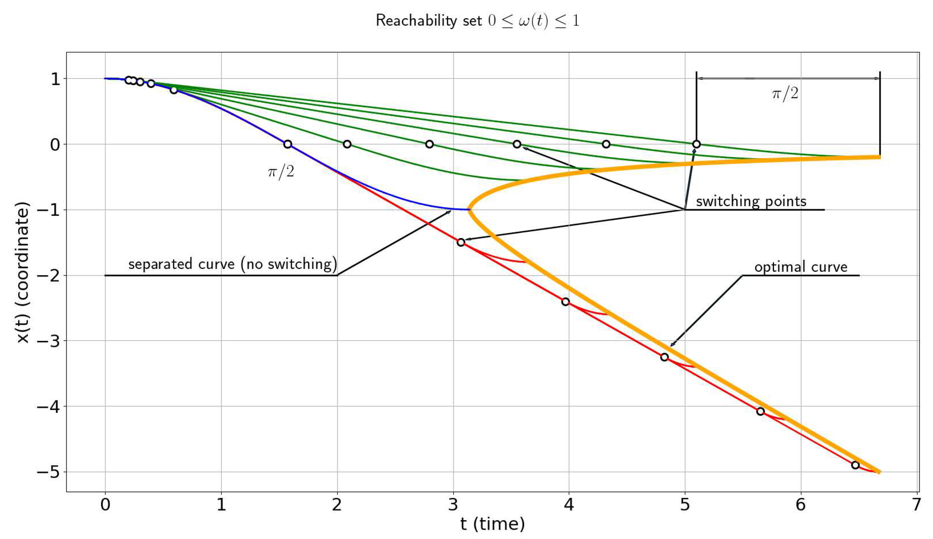
Figure 2. Complete reachability set of all possible optimal trajectories.

0 \leq ω \leq 1, A = 1, B \in [0.2, 5] .

Any points with

x = 0

can be reached in 4 switches (eq. (10)).

Figure 2. Complete reachability set of all possible optimal trajectories.

0 \leq ω \leq 1, A = 1, B \in [0.2, 5] .

Any points with

x = 0

can be reached in 4 switches (eq. (10)).

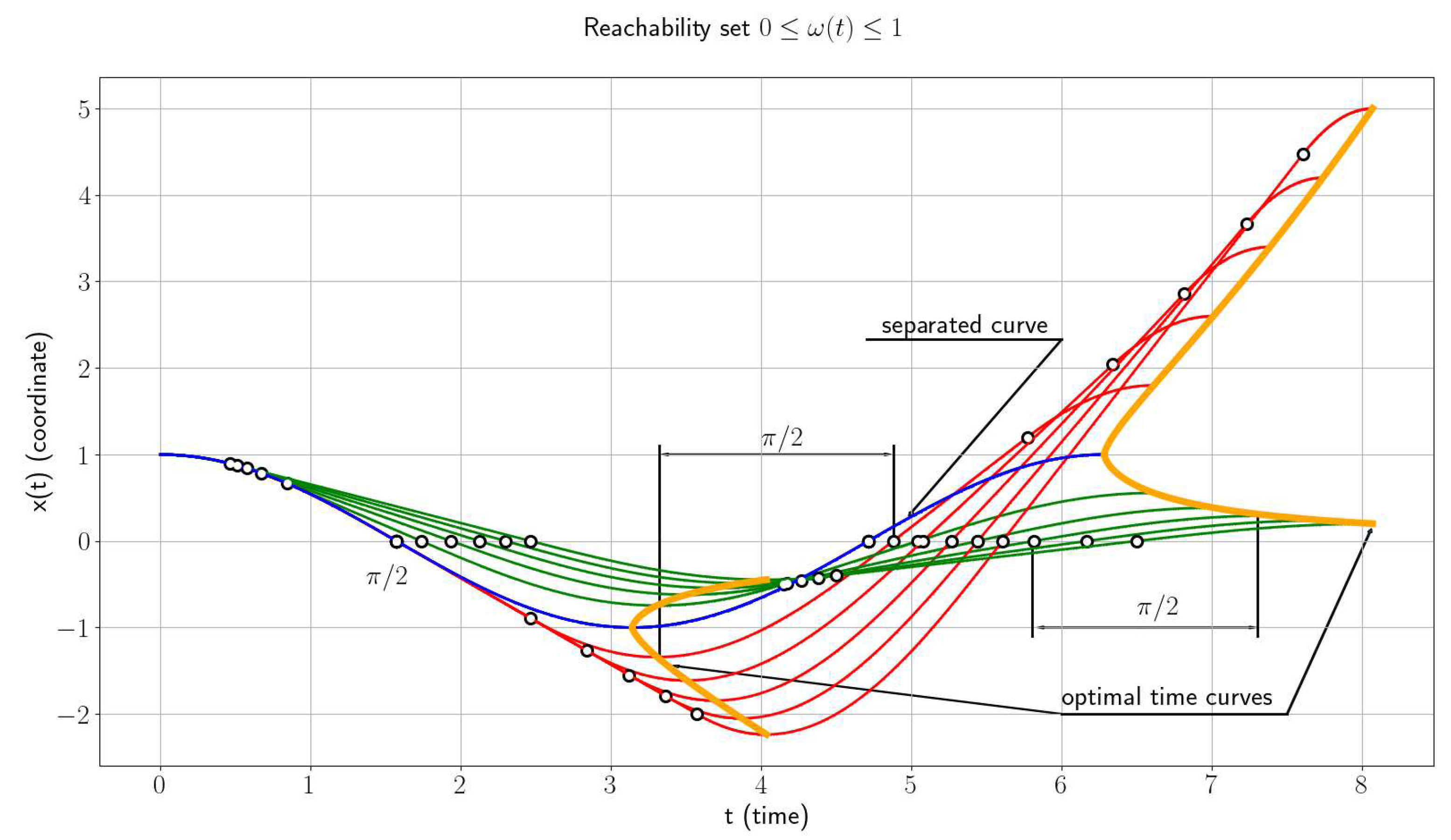
Figure 3. The initial guess of

ω (t) .

The plot a) refers to the optimal case (23), the case b) refers to the non-optimal solution (24).

Figure 3. The initial guess of

ω (t) .

The plot a) refers to the optimal case (23), the case b) refers to the non-optimal solution (24).

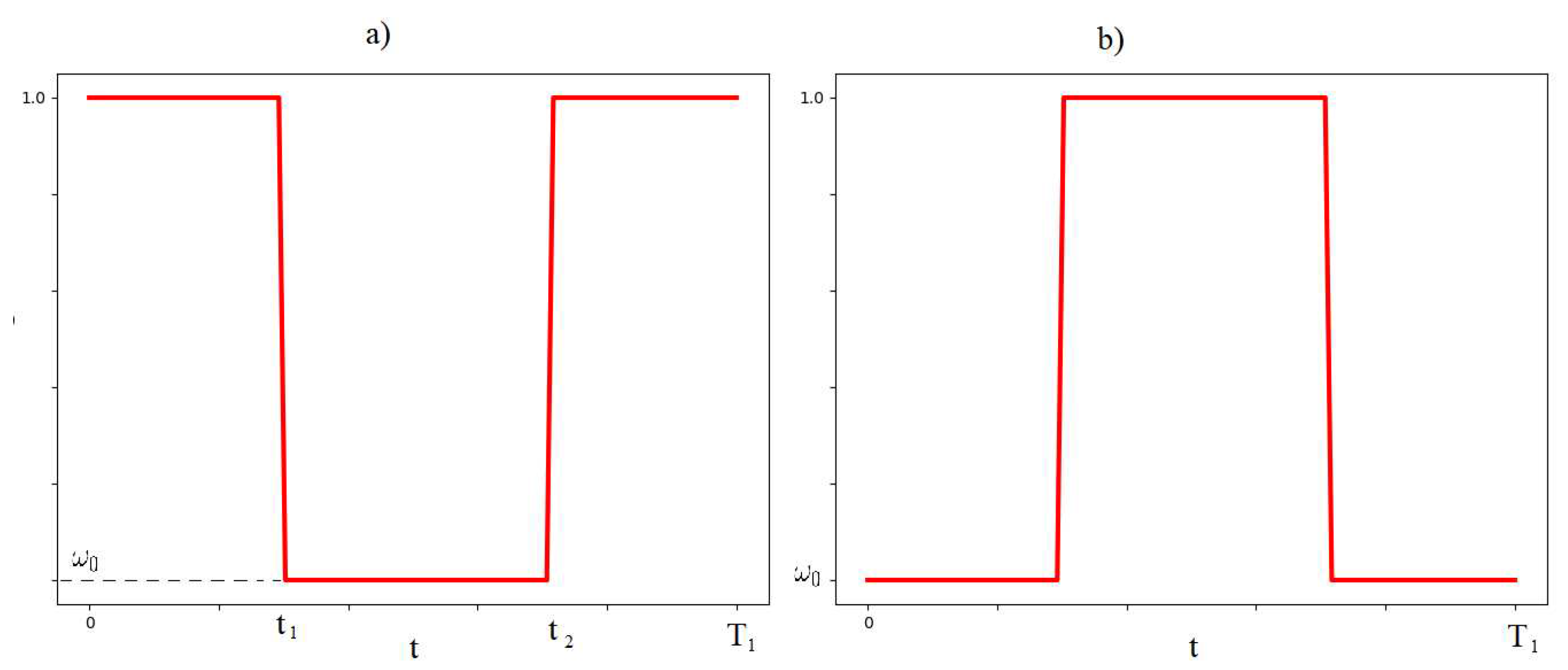
Figure 4. Complete reachability set of all possible optimal trajectories.

0.75 \leq ω \leq 1, A = 1 .

Number of switching points depends on terminal conditions. Within a single oscillation there are 4 switching points.

Figure 4. Complete reachability set of all possible optimal trajectories.

0.75 \leq ω \leq 1, A = 1 .

Number of switching points depends on terminal conditions. Within a single oscillation there are 4 switching points.

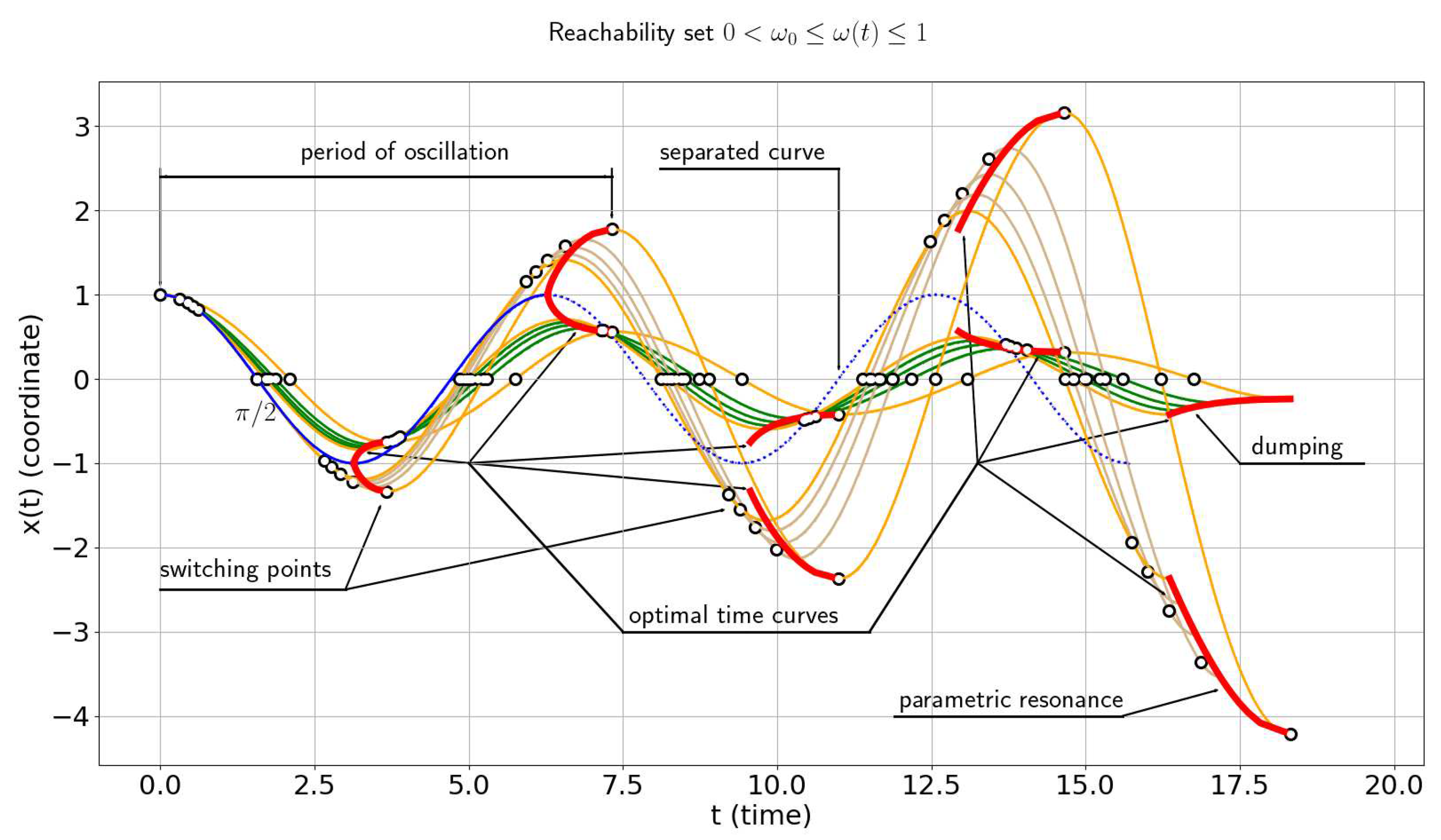
Figure 5. A time optimal trajectory of oscillations

a)

and the phase portrait

b)

with switching points

x (0) = 1, \dot{x} (0) = 0, x (T) = 8, \dot{x} (T) = 0, 0.5 \leq ω (t) \leq 1, T \approx 14.97 .

Figure 5. A time optimal trajectory of oscillations

a)

and the phase portrait

b)

with switching points

x (0) = 1, \dot{x} (0) = 0, x (T) = 8, \dot{x} (T) = 0, 0.5 \leq ω (t) \leq 1, T \approx 14.97 .

Disclaimer/Publisher’s Note: The statements, opinions and data contained in all publications are solely those of the individual author(s) and contributor(s) and not of MDPI and/or the editor(s). MDPI and/or the editor(s) disclaim responsibility for any injury to people or property resulting from any ideas, methods, instructions or products referred to in the content.

© 2023 by the authors. Licensee MDPI, Basel, Switzerland. This article is an open access article distributed under the terms and conditions of the Creative Commons Attribution (CC BY) license (http://creativecommons.org/licenses/by/4.0/).

Copyright: This open access article is published under a Creative Commons CC BY 4.0 license, which permit the free download, distribution, and reuse, provided that the author and preprint are cited in any reuse.

Alerts

MDPI Initiatives

Important Links

Choose an area of interest and we will send you notifications of new preprints at your preferred frequency.

Disclaimer

Inverse Problem to Control the Coefficient of a Differential Equation in Time

Abstract

Keywords:

Subject:

1. Introduction

2. Preliminaries and problem formulation

3. Symmetry of the problem

4. Analysis with 0 ≤ ω ≤ 1

4.1. Different sign values at the boundary

4.2. Proof of optimality

4.3. Identical sign values at the boundary

5. Problem with ω > 0

5.1. Construction of an analytical solution when ω > 0

6. Construction of the optimal solution

7. Proof of optimality and final solution

8. General case

9. Construction of the set of reachability

10. Conclusions and outlook

11. Declaration of competing interest

References

MDPI Initiatives

Important Links

Subscribe

4. Analysis with $0 \leq ω \leq 1$

5. Problem with $ω > 0$

5.1. Construction of an analytical solution when $ω > 0$