1. Introduction
The load density increases even more with the inclusion of different loads passing through the electrical networks [
1]. Consequently, the complexity of the electric network is further increased. Under these conditions the stability of power systems must be ensured, and distributed generation plants contribute significantly to improving the stability. Especially the increase in environmental factors on transmission and distribution lines increases the importance of distributed generation plants (DGP) on energy security [
2]. Photovoltaic systems and wind energy systems are generally used for distributed generation plants. Since inverters are used in these systems, harmonic distortion rates in the network increase [
3,
4,
5,
6,
7,
8]. In electricity networks, 3rd, 5th, 7th and 9th order harmonics occur due to DGP and total harmonic distortion is seen around 20% [
9]. Generally, 5th and 7th order harmonics occur in wind farms. In cases of unbalanced loading, 3rd and 9th order harmonics are also seen [
10,
11,
12,
13,
14,
15]. In photovoltaic systems, 3rd, 7th and 9th order harmonics are dominant and the total harmonic distortion is around 20% [
16]. While 5th and 7th order harmonics have positive component character, 3rd and 9th order harmonics have zero sequence character [
17]. Many connections in electrical facilities are made with cables. Especially the connection of DGP to the electricity network is made with high voltage power cable (HVPC). Thus, HVPC faults are important issue for DGP. HVPC occurs from insulation layer, semiconductor layer, metal sheath, buffer layer and armour respectively. The most important layer in HVPC is the insulation layer because the insulating layer prevents short circuits by covering the conductor. Hence, HVPC faults usually occur in the insulating layer. The most important factor for insulation faults is insulation aging. High electrical stress and high temperature in the insulation layer are causes of insulation aging [
18,
19,
20]. The metal part of HVPC is grounded to restrict high electrical stress. These metal parts are metal sheath and armour. However, when metal parts of the cable are grounded the sheath current (SC) flows on the metal parts of the cable. SC induces in the metal parts of the cable due to the load current, just like in the transformer. Also, SC can be up to 50% of line current. As this will cause a lot of energy loss, it causes an increase in temperature in the cable [
21]. The cable temperature according to SC is shown in
Table 1. PVC and XLPE insulation materials are generally used in HVPC. The endurance temperature of XLPE insulation material is 90ºC, and that of PVC insulation material is 70ºC. As can be seen from
Table 1, insulating materials will be damaged at high SC.
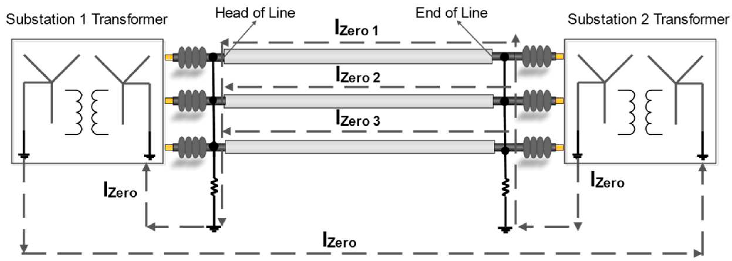
In addition to SC, harmonic currents and zero sequence currents cause malfunctions in high voltage power cables. Harmonic currents generally occur due to power electronic devices, and cable temperature increases due to harmonic currents. Also, parallel resonance occurs due to harmonics, and extremely insulation voltage occurs due to parallel resonance. The most important causes of zero sequence currents, which are composed of cable metal parts, are unbalanced load currents and cable configuration. In unbalanced load current case, the sum of currents at the cable grounding point is different from zero and the residual current flows through the metal parts of the cable as zero sequence current. This case is shown in
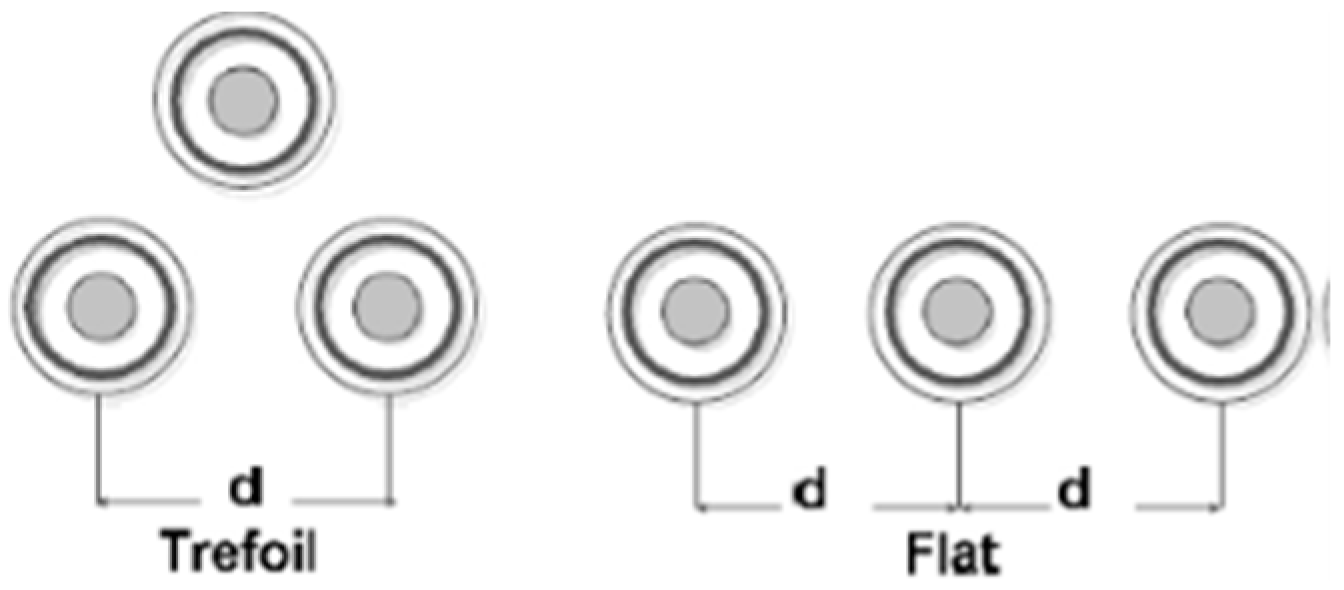
Figure 1. Even if the line current is balanced, zero sequence current occurs in the metal parts of the cable due to the cable configuration. The cable configurations used in the application are trefoil and flat. These arrangements are shown in
Figure 2.
Since the distances between the cables are equal in trefoil arrangement, the inductance and capacitance of the cables are equal. However, since the distance between the cables is not equal in a flat arrangement, the inductance and capacitance of the cable are not equal. Therefore, zero sequence currents flow in the metal parts of the cable due to unbalanced currents, and flat formation is generally used in the practice [
22,
23]. Especially with the increase in cable length, cable capacitance also increases. Increasing capacitance of the cable further increases the effect of these currents. For example, 800 A sheath current occurs in the metal part of high voltage cable that has 30 km long in wind farm [
24]. As a result of the research, cable failures are mostly seen in cable accessory points [
25]. Cable joints and cable terminations are the most important cable accessories. Single-point bonding, solid bonding and cross bonding methods are used in today's practice for grounding of high voltage cable metallic parts to prevent cable insulation faults. However, since these grounding methods are not sufficient in systems with high harmonic and zero sequence currents because these factors are not considered when these methods are designed, so cable faults cannot be prevented sufficiently [
26].
2. Materials and Methods
In this study, the material and method section consists of two stages. First of all, a grounding method has been introduced to prevent insulation failures in the high voltage cable due to different factors. Then, how the proposed grounding method is optimized with artificial intelligence methods is introduced.
2.1. The suggested high voltage cable grounding method
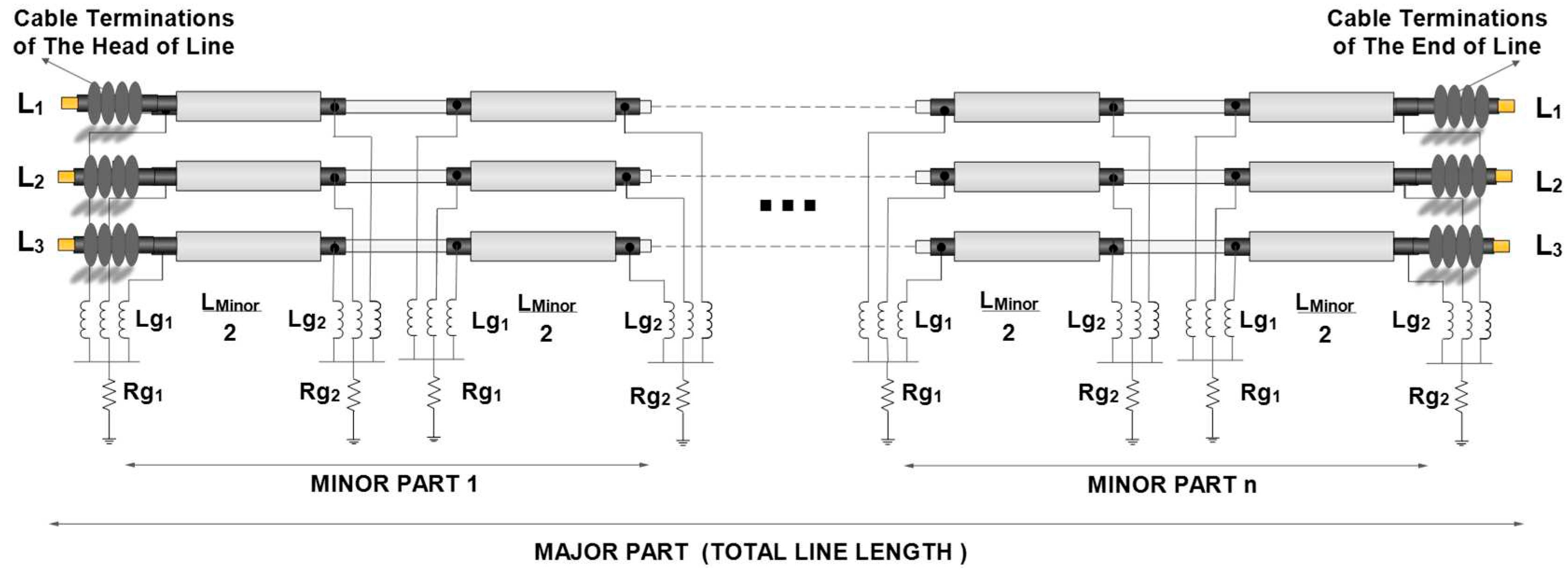
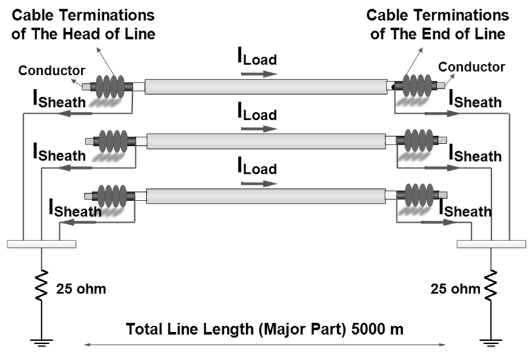
In this study, SSBLR method is designed as a new high voltage power cable grounding method to prevent the sheath current and voltage effects, harmonic current effects, and zero sequence current effects. This cable grounding method is shown in
Figure 3.
In SSBLR method, the total cable length is called a major part, and the major part occurs from minor parts. These minor part parameters are determined by the optimization methods. There are different optimization problems in determining minor part parameters. These optimization problems are minimization of current harmonic distortion (MHC), the induced voltage (MV), and the induced current (MC) on the metal parts of the cable. In practice, cable sheath and armour are usually grounded. therefore, the total current flowing through the armour and cable is defined as the metal part current (MC). Minor part parameters are minor part length (L), grounding resistances (Rg1 and Rg2), and grounding inductances (Lg1 and Lg2), and optimum minor part parameters should provide optimum MV, MC, and MHC values.
2.2. Optimization process of the suggested high voltage cable grounding method
It is seen that optimization of minor part parameters is a multi-objective optimization problem. The most widely used multi objective optimization methods are Pareto Optimal, Scalarization method and Vector Computational Genetic Algorithm [
27,
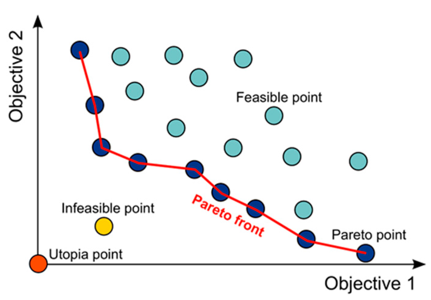
28]. In this study, Pareto optimal method is used as multi-objective optimization method. In Pareto optimal method, there are dominant and non-dominant solutions. These solutions are shown on Pareto front, and the most suitable solution is determined with Pareto optimal. This Pareto front is shown in
Figure 4 [
29]. In this study, many optimal solutions are obtained, so Pareto optimal method is selected as multi-objective optimization method to determine the most suitable solution.
These solutions are classified as dominant and non-dominant solutions by Pareto optimal method. Thus, the most suitable solution is determined by Pareto front. Optimum MV, MC, and MHC values that are determined according to optimum minor part parameters (L, Rg1, Rg2, Lg1 and Lg2 values) are used determination of Pareto front, and the objective function is necessary to solve optimization problems. The prediction methods are used as the objective function to solve optimization problems in this study. Minor part parameter values are given as input parameters, and the predicted MV, MC, and MHC values are used as output parameters. Namely, MV, MC, and MHC values are objective function values in the optimization problem.
2.3. Usage of the prediction methods in Optimization process
The prediction methods are artificial neural networks, hybrid artificial neural networks and regression methods. These methods are used as objective function because these methods are widely used for the forecasting studies in electrical engineering [
30,
31,
32,
33,
34,
35,
36]. In hybrid artificial neural networks, the weights of artificial neural network are updated by optimization method [
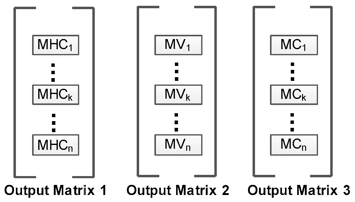
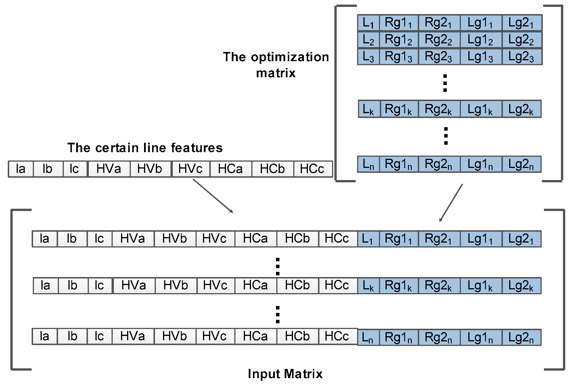
37]. The prediction methods should be trained with the training data to predict MV, MC, and MHC values. Training data are the input and output matrices. In this study, there are three optimization problems, and each the prediction method should be trained for each optimization problem. Namely, the prediction method should be trained for prediction of MV, MC, and MHC separately. Thus, there are three output matrices for MV, MC, and MHC in training of the prediction method. Also, the input matrix is common for each optimization problem. The input matrix is generated with vectors, and a vector occurs from minor part length (L), grounding resistances (Rg1 and Rg2), grounding inductances (Lg1 and Lg2), three-phase line currents (Ia,Ib,Ic), voltage harmonic distortions of each phase (HDVa, HDVb, HDVc), current harmonic distortions of each phase (HDCa, HDCb, HDCc). The input matrix is shown in
Figure 4, and the output matrices are shown in
Figure 5.
When the prediction method is trained for MHC prediction, the input matrix and output matrix 1 are used that is shown in
Figure 6. When the prediction method is trained for MV prediction, the input matrix and output matrix 2 are used. When the prediction method is trained for MC prediction, the input matrix and output matrix 3 are used.
Primarily, optimum minor part parameters are determined according to the predicted most suitable MV value. In MV prediction, the input matrix and output matrix 2 are used for the training of the prediction method. After the training of the prediction method, the optimum minor part parameters are determined according to the predicted most suitable MV value. Thus, a new input matrix is necessary for minor part optimization. The generation of this input matrix is shown in
Figure 7.
It is seen that when the input matrix is generated, the optimization matrix is used to generate the vector for the input matrix. Namely, the optimum minor part values are researched in the optimization matrix, and the optimization matrix is updated by optimization methods. Hence, a vector for the input matrix is generated by unify of the certain line features and a vector of the optimization matrix. After the input matrix is generated, MV values of the vectors are predicted according to
Figure 8.
2.4. Optimum minor part detection process for the suggested method
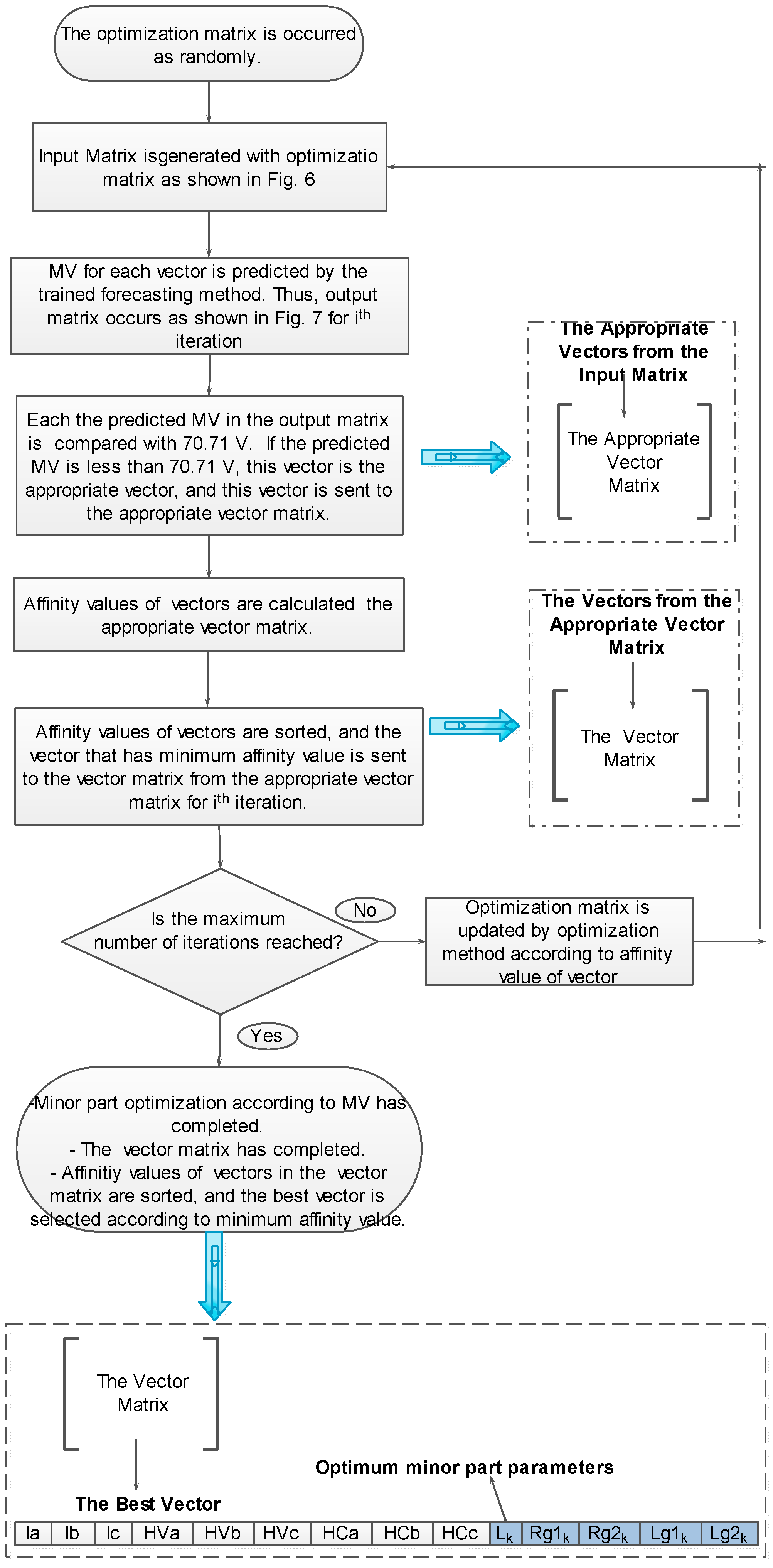
Optimum minor parameters are determined the optimization algorithm that is shown in
Figure 9 according to the predicted most suitable MV value. In this study, the most suitable MV is determined according to affinity value, and affinity value is calculated with touch voltage limit and the predicted MV of the vector. Where touch voltage limit is for person is 70.71 V (peak) according to IEC 479-1 standard. Affinity value (AV) shows vector quality, and affinity value is calculated by (1) in the optimization algorithm. Where 70.71 V is touch voltage limit for person. Namely the most suitable predicted MV value has minimum affinity value.
The optimum parameter determination for the grounding method proposed in this study is done with the multi-objective optimization method. Optimum grounding parameters for the proposed method were first determined by MV optimization. However, these parameter values must also be appropriate for MC and MHC, so many optimal solutions are necessary for pareto front. Thus, many optimum minor parameters are determined according to the most suitable MV values on the pareto front. These optimum minor part parameters are the dominant solutions, and these dominant solutions are compared to select the most dominant solution on the pareto front.
The most dominant solution is the most suitable optimum minor part parameters, and MC and MHC values should also be minimized with the most suitable optimum minor part parameters. Namely, the selection of the most dominant solution is made according to MC and MHC minimization. MV is more dependent on the minor part length than the minor part parameters. Namely, as the length of the minor part increases, MV increases even more. If the length of the minor part is short, MV will also be low. However, if the length of the minor part decreases to reduce MV, the number of minor parts increases. In this case, grounding will not be economical as the number of parts will increase. As can be seen, the length of the minor part should be as large as possible for an economical grounding. This length is limited by MV. Therefore, the closer MV is to the touch voltage, the greater the minor part length will be. In other words, the smaller the affinity value for MV, the greater the length of the minor part and the less the number of minor parts, so the grounding will be more economical and technical.
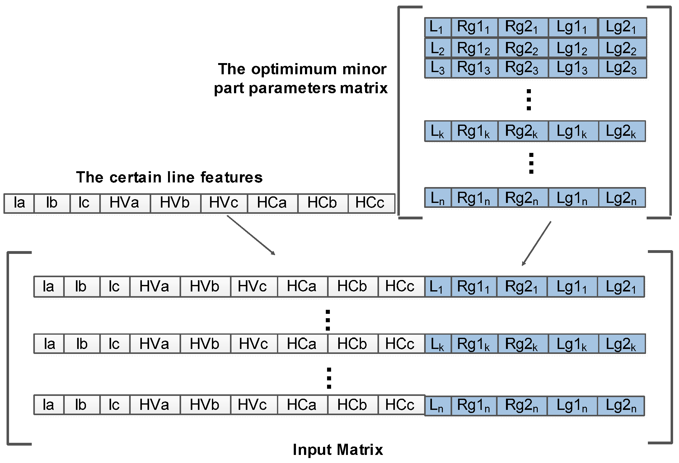
The Pareto front is occurred with the estimated MC and MHC. MC and MHC values are estimated by the optimum minor part parameters that are determined MV value. Before MC and MHC estimation studies for the pareto front, the prediction method should be trained. An input matrix is necessary for MC and MHC estimation studies. This input matrix is the input matrix used for MV training. The input matrix and output matrix 1 are used when the prediction method is trained for MHC. The input matrix and output matrix 3 are used when the prediction method is trained for MC. After the prediction method is trained for MC or MHC, MC or MHC prediction are made to occur the pareto front. Also, a new input matrix is necessary for the prediction of MC and MHC. Many the optimum minor part parameters are determined with the most suitable MV values, and the optimum minor part parameters matrix is generated for the input matrix. The vectors for input matrix are generated with the optimum minor part parameters matrix and certain line features as seen in
Figure 10. The prediction process of MC or MHC is shown in
Figure 11.
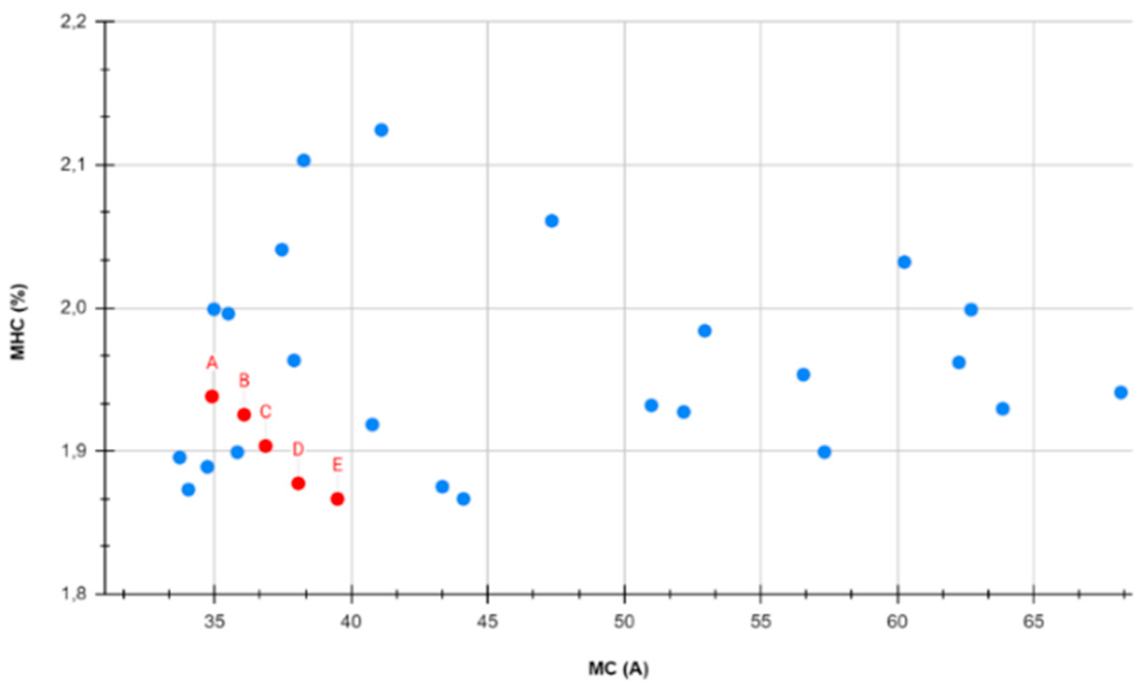
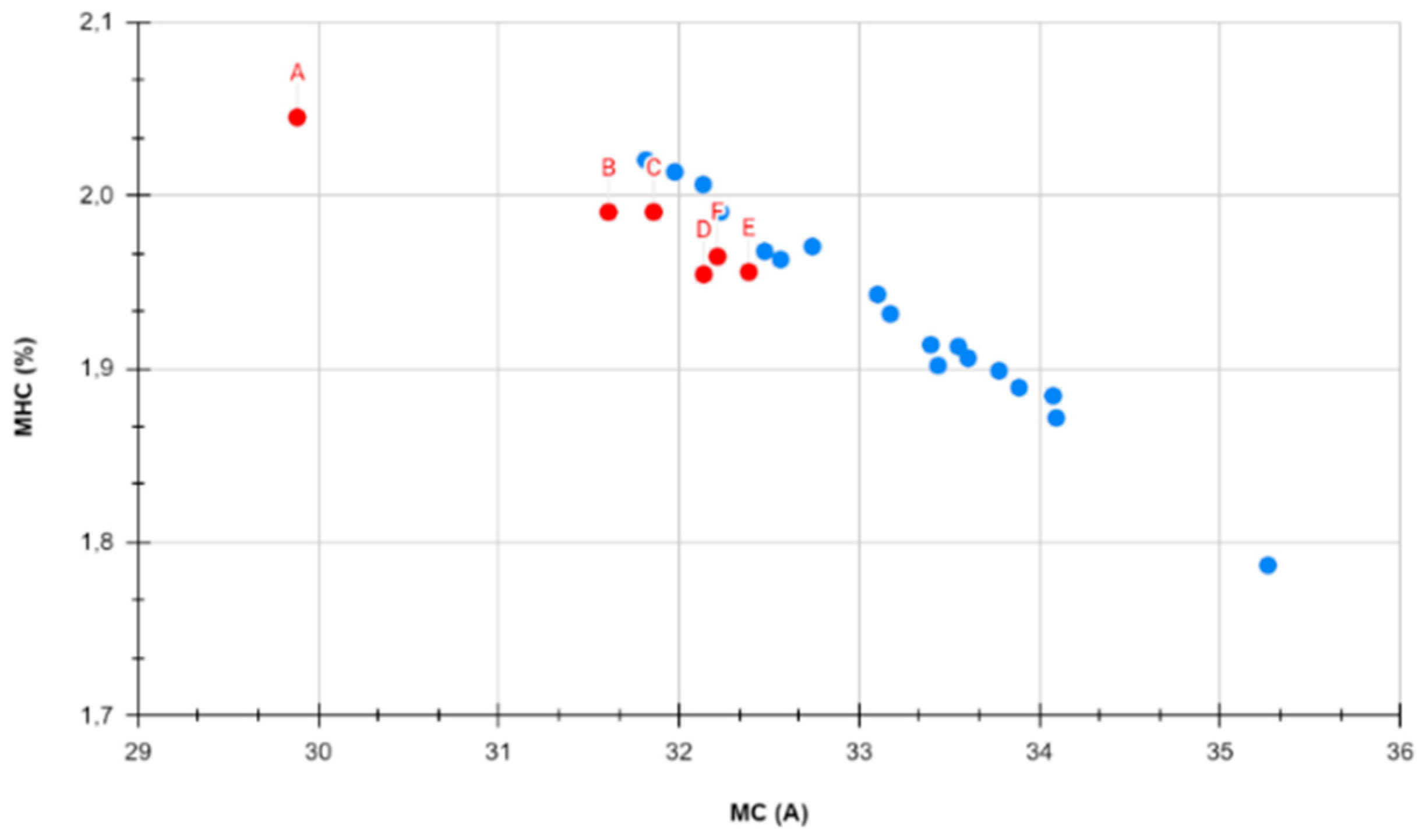
The predicted MC and MHC values are marked in Pareto graphic as shown in
Figure 4. Thus, pareto front is occurred by different MC and MHC values. The most dominant solution is found among the optimal results on the Pareto front. Therefore, the most suitable minor part parameter values for the grounding of high voltage cables are determined by Pareto front.
3. Results and Discussion
Simulation studies are carried out to see the effects of the optimum grounding parameters found by the multi-objective optimization method on the line and to find the best method. A 5 km long high voltage cable line was selected for simulation studies. Additionally,
Table 2 contains information about the current and voltage values of the line.
Primarily, bonding of high voltage cable line is made with the bonding method that is indicated in the literature. In the literature, single point bonding, solid bonding and cross bonding methods are indicated according to IEEE 575-1988 standard. The most important factor is MV, and MV of solid bonding is less than single point bonding and cross bonding. Thus, bonding of high voltage cable line is made with solid bonding to compare the suggested the optimized SSBLR method. The solid bonding that is shown in
Figure 12 is used for the same high voltage line, and the result of solid bonding is shown in
Table 3.
It is seen in
Table 3 that MV, MC and MHC extremely increases at the cable termination points. In this case, the cable temperature extremely increases according to
Table 1. Thus, cable insulation faults and electroshock risk occur when the solid bonding is used as the bonding method for long high voltage lines in the distributed generation plants.
3.1. Training process for the prediction methods in optimization of the suggested method Subsection
It is seen that the solid bonding is not suitable for bonding of high voltage cable line. Thus, optimum SSBLR method is designed. The data that are used in optimization studies of SSBLR method are obtained from PSCAD/EMTDC simulation program. 54 different high voltage power cable lines are simulated, and MC, MV, and MHC values of these lines are measured in PSCAD/EMTDC. These measured data are used in the training studies of the prediction methods. The input matrix occurs from 54x14 matrix. Namely, the input parameters are Ia, Ib, Ic, HDVa, HDVb, HDVc, HDCa, HDCb, HDCc, L, Rg1, Rg2, Lg1 Lg2. Output matrices are 54x1 matrices for MV, MC, MHC. Namely, output matrices occur from the measured MV, MC, MHC in PSCAD/EMTDC. Primarily, the prediction methods are trained for MV, and the trained prediction methods that have minimum training errors are used to determine optimum minor part parameter with MV. Three types of prediction methods are used to determine the most suitable prediction method. These methods are artificial neural networks (ANN), hybrid artificial neural networks (H-ANN) and regression methods. Feed forward back propagation, Elman Neural Network and Narx are compared for ANN. The raining error of FFBP is 344.1, the training error of ENN is 76.76, and the training error of Narx is 265.65. In H-ANN, the weights of ANN are updated by optimization method. The used optimization methods to update weight of ANN are genetic algorithm (GA), particle swarm optimization (PSO), and gravitational search algorithm (GSA). Thus, H-GA, H-PSO, and H-GSA methods are generated. The training error of H-GA is 1.769, the training error of H-PSO is 3.449, and the training error of H-GSA is 2.36. Exponential gaussian regression (EGR), squared exponential gaussian regression (SEGR), and matern 5/2 gaussian regression (MGR) are used for regression. The training error of EGR is 6.66, the training error of SEGR is 5.05, and the training error of MGR is 4.60. The prediction methods are selected according to minimum training error. ENN, H-GA, and MGR are selected from each group according to their training error value. Also, genetic algorithm (GA), particle swarm optimization (PSO), and gravitational search algorithm are used as the optimization methods. These optimization methods are used for optimization of the optimization matrix that is shown in
Figure 7.
3.2. Determination of the optimum grounding parameters with Pareto Optimal for different cases
In this study, 7 different cases are evaluated to determine the optimum parameters for the proposed grounding method using the Pareto optimal method. In each case, a different estimation method is used with a different optimization method. Optimum grounding parameters are obtained with these methods. Then, for each case, the grounding parameters obtained by the Pareto optimal method were simulated on the line and their suitability is checked.
Case 1
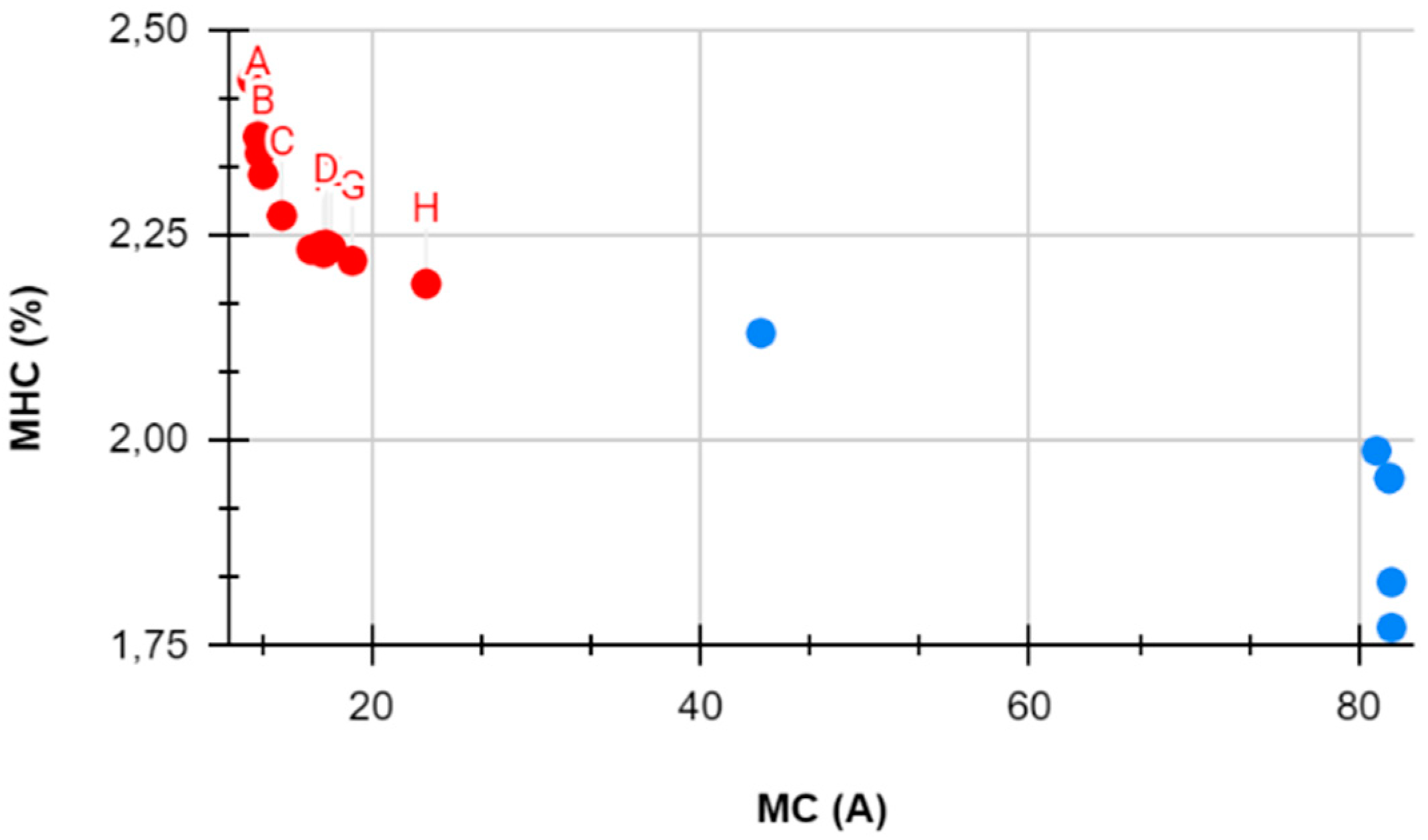
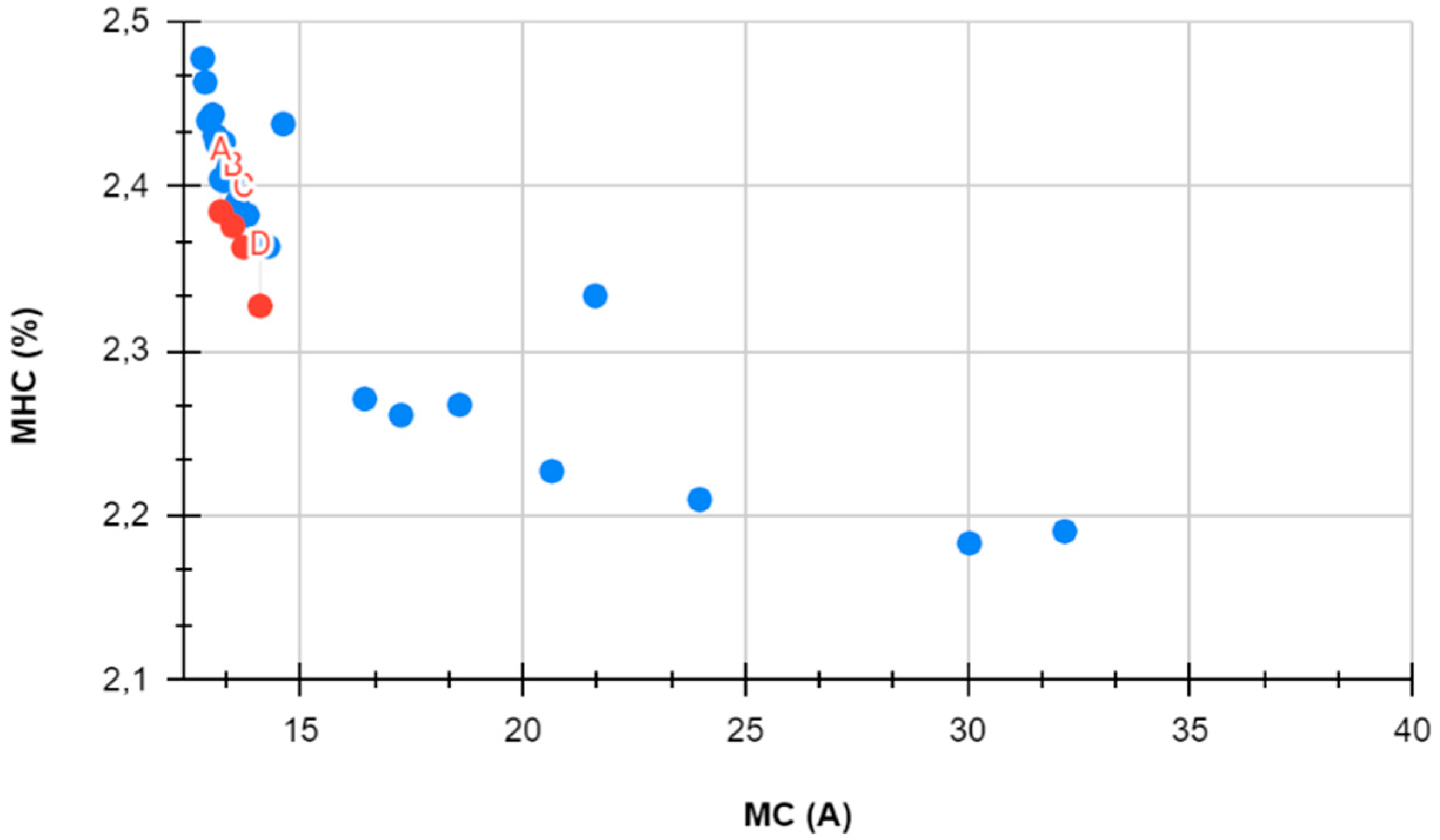
When ENN is used as the objective function, and GA is used as the optimization method, the optimum minor part parameters are determined with the most suitable MV values. MC and MHC values of the vectors are predicted to occur the pareto front. In the
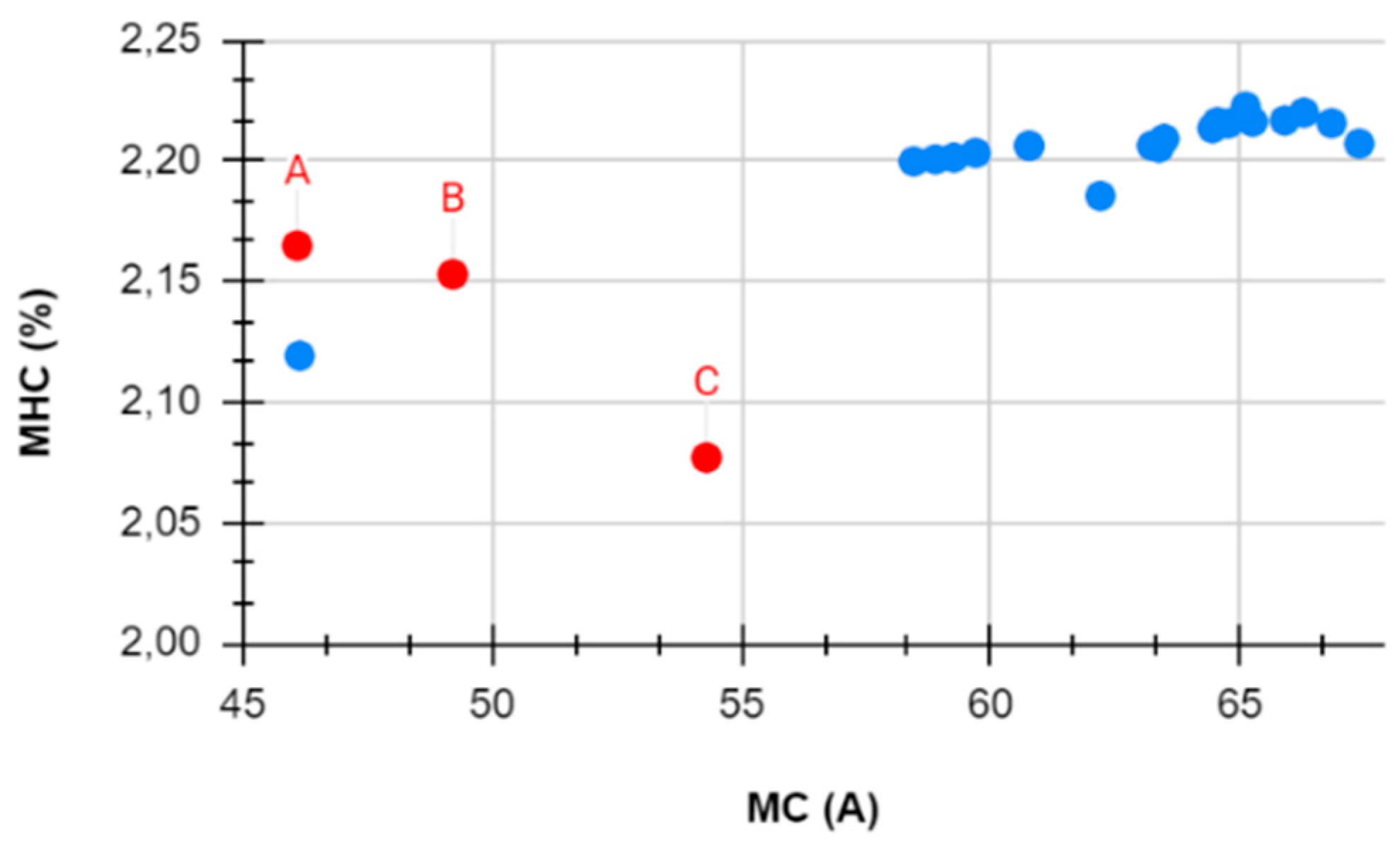
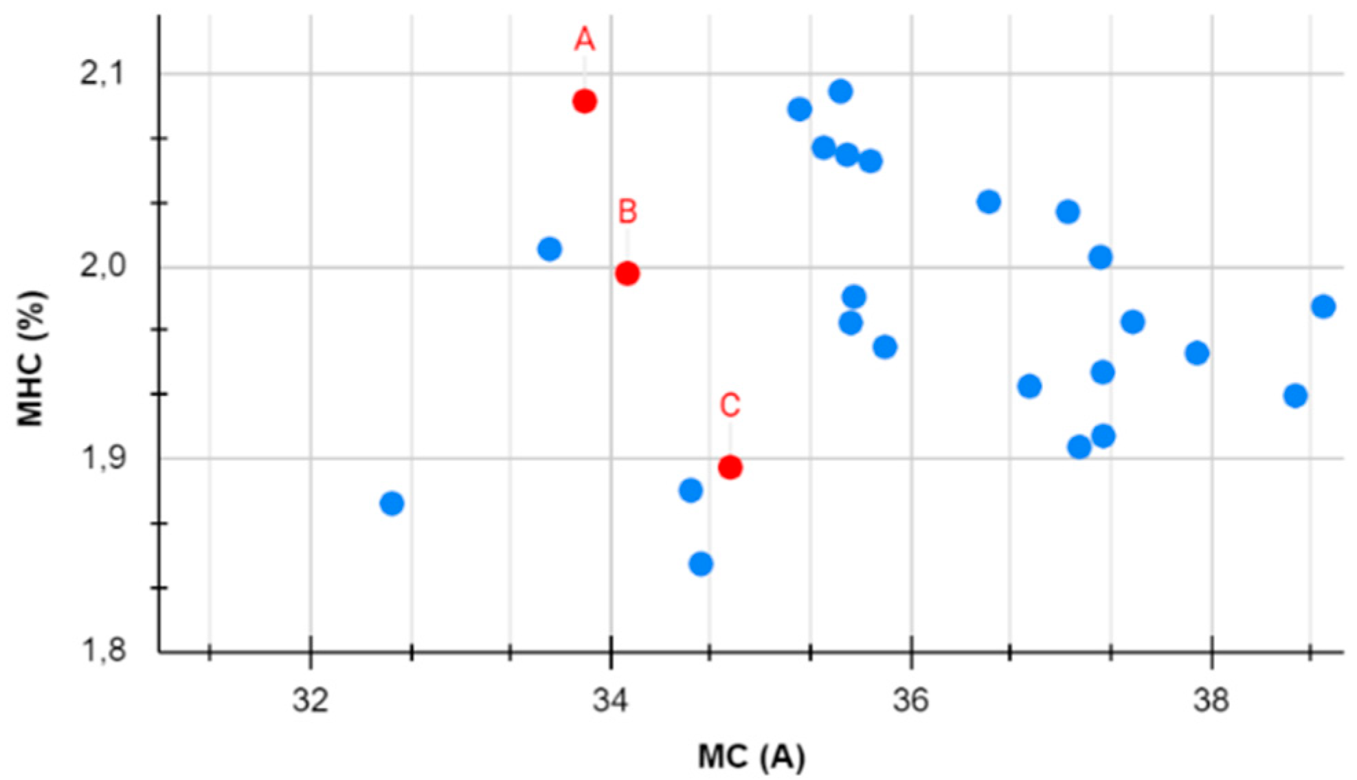
Figure 13, the predicted MC and MHC values are shown, and each dot in
Figure 12 presents a vector that is in the input matrix, and red dots present the pareto front. The optimum minor part parameters that are on the pareto front vectors are seen in
Table 4.
Case 2
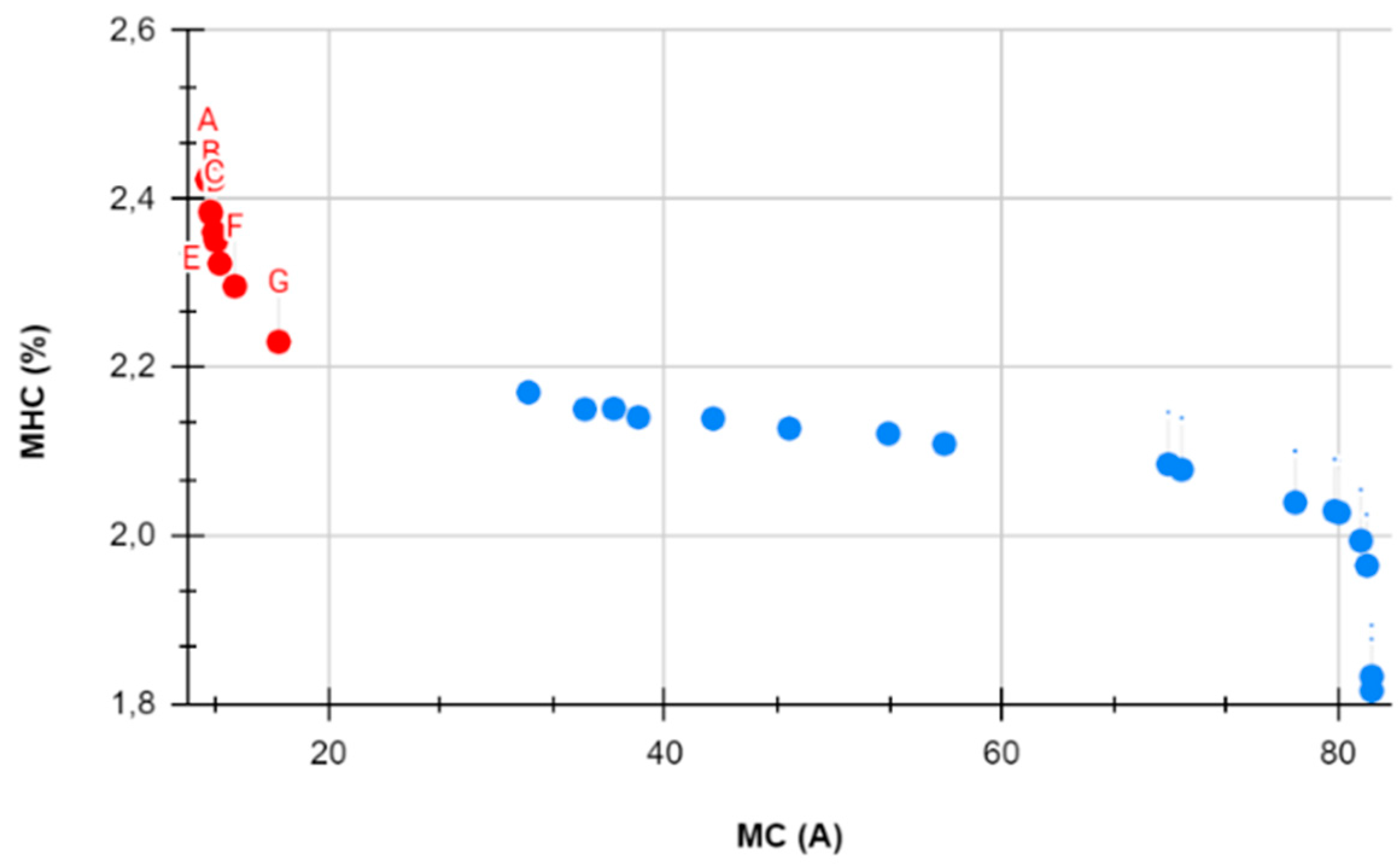
When ENN is used as the objective function, and PSO is used as the optimization method, the optimum minor part parameters are determined with the most suitable MV values, and then MC and MHC values of the vectors are predicted. The predicted MC and MHC values and the pareto front are shown in
Figure 14. The optimum minor part parameters that are on pareto front vectors are shown in
Table 5.
Case 3
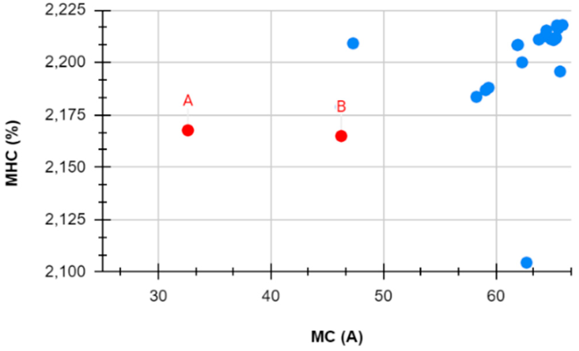
When ENN is used as the objective function, and GSA is used as the optimization method, the optimum minor part parameters are determined. After the minor part parameters are determined, MC and MHC values of the vectors are predicted, and pareto front is occurred as shown
Figure 15. The optimum minor part parameters on the pareto front are shown in
Table 6.
Case 4
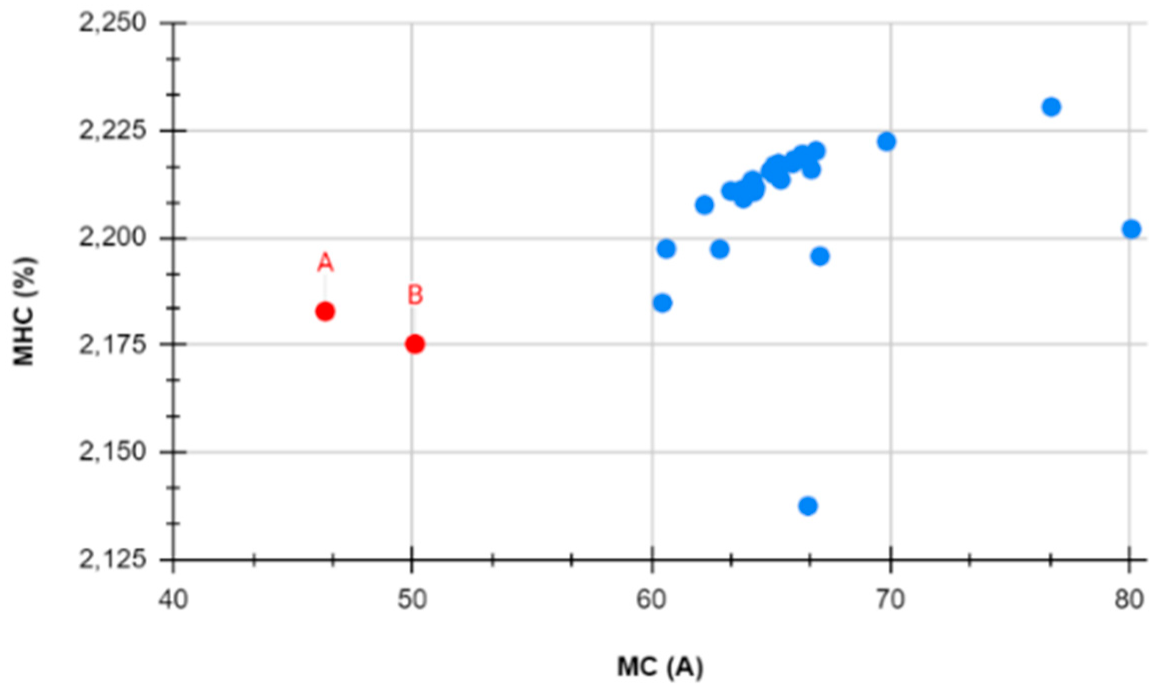
When MGR is used as the objective function, and GA is used as the optimization method, the optimum minor part parameters are determined. After the minor part parameters are determined, MC and MHC values of the vectors are predicted, and the pareto front is occurred as shown
Figure 16. The optimum minor part parameters on the pareto front are shown in
Table 7.
Case 5
When MGR is used as the objective function, and PSO is used as the optimization method, the optimum minor part parameters are determined. After the minor part parameters are determined, MC and MHC values of the vectors are predicted, and the pareto front is occurred as shown
Figure 17. The optimum minor part parameters on the pareto front are shown in
Table 8.
Case 6
When MGR is used as the objective function, and GSA is used as the optimization method, the optimum minor part parameters are determined. After the minor part parameters are determined, MC and MHC values of the vectors are predicted, and the pareto front is occurred as shown Figure 18. The optimum minor part parameters on the pareto front are shown in
Table 9.
Figure 18.
Pareto front and the predicted MC and MHC values.
Figure 18.
Pareto front and the predicted MC and MHC values.
Case 7
When H-GA is used as the objective function, and GA is used as the optimization method, the optimum minor part parameters are determined. After the minor part parameters are determined, MC and MHC values of the vectors are predicted, and pareto front is determined as shown in Figure 18. The optimum minor part parameters on the pareto front are shown in
Table 10.
Figure 18.
Pareto front and the predicted MC and MHC values.
Figure 18.
Pareto front and the predicted MC and MHC values.
Case 8
When H-GA is used as the objective function, and PSO is used as the optimization method, the optimum minor part parameters are determined. After the minor part parameters are determined, MC and MHC values of the vectors are predicted, and pareto front is determined as shown in
Figure 19. The optimum minor part parameters on the pareto front are shown in
Table 11.
Case 9
When H-GA is used as the objective function, and GSA is used as the optimization method, the optimum minor part parameters are determined. After the minor part parameters are determined, MC and MHC values of the vectors are predicted, and pareto front is determined as shown in
Figure 20. The optimum minor part parameters on the pareto front are shown in
Table 12.
4. Simulation results for different cases
The obtained optimum minor part parameters on the pareto front are simulated in PSCAD/EMTDC, and MV, MC and MHC values of these vectors are measured to determine dominant solution on the pareto front.
Simulation results for Case 1
The simulation results of pareto front vectors are shown in
Table 13. The measurements of these values are made at head of line (HL) and end of line (EL) points. Where 1, 2 and 3 present each phase (L1, L2 and L3) in high voltage cable line. The dominant solution on the pareto front is determined according to MV, MC and MHC values. Primarily, MV values of vectors are compared with touch voltage limit, and the vectors whose MV are lower than the touch voltage are selected. These vectors are C, D, F, G and H vectors, and then, MC values of these vectors are compared. MHC values of these vectors are near each other’s. The lowest MC value belongs to the H vector. Thus, dominant solution is H vector in Case1.
Simulation results for Case 2
The simulation results of pareto front vectors for Case 2 are shown in
Table 14. MV values of vectors are compared with touch voltage limit, and it is seen that only MV of D vector is lower than touch voltage limit. Thus, dominant solution is D vector in Case 2.
Simulation results for Case 3
The simulation results of the pareto front vectors for Case 3 are shown in
Table 15. MV values of vectors are compared with touch voltage limit, and the vectors whose MV are lower than the touch voltage are D, E, F and G vectors, and then, MC values of these vectors are compared. MHC values of these vectors are near each other’s. The lowest MC value belongs to the F vector. Thus, dominant solution is F vector in Case 3.
Simulation results for Case 4
The simulation results of the pareto front vectors for Case 4 are shown in
Table 16. MV values of vectors are compared with touch voltage limit, and it is seen that there is no vector whose MV is lower than the touch voltage. Thus, there is no suitable solution in Case4.
Simulation results for Case 5
The simulation results of the pareto front vectors are shown in
Table 17. The simulation results of Pareto front solutions MV values of vectors are compared with touch voltage limit, and it is seen that there is no vector whose MV is lower than the touch voltage. Thus, there is no suitable solution in Case 5.
Simulation results for Case 6
The simulation results of pareto front vectors for case 6 are shown in
Table 18. MV values of vectors are compared with touch voltage limit, and it is seen that only MV of A vector is lower than touch voltage limit. Thus, dominant solution is A vector in Case 6.
Simulation results for Case 7
The simulation results of pareto front vectors for case 7 are shown in
Table 19. MV values of vectors are compared with touch voltage limit, and the vectors whose MV is lower than the touch voltage are A, B, and C vectors, and then, MC and MHC values of these vectors are compared. The lowest MHC and MC values belong to the B vector. Thus, dominant solution is B vector in Case 7.
Simulation results for Case 8
The simulation results of pareto front vectors are shown in
Table 20. MV values of vectors are compared with touch voltage limit, and the vectors whose MV is lower than the touch voltage are A, B, C, D and E vectors, and then, MC and MHC values of these vectors are compared. The lowest MC and MHC values belong to the B vector. Thus, dominant solution is B vector in this section.
Simulation results for Case 9
The simulation results of pareto front vectors are shown in
Table 21. MV values of vectors are compared with touch voltage limit, and the vectors whose MV is lower than the touch voltage are A, B, C, D, E and F vectors, and then, MC and MHC values of these vectors are compared. The lowest MC values belongs to the A vector. Thus, dominant solution is A vector in Case 9.
5. Discussion
After creating the Pareto optimum front for each case, the dominant vectors forming this front are determined according to the simulation results. Vector H for Case 1, vector D for Case 2, vector F for Case 3, vector A for Case 6, vector B for Case 7, vector B for Case 8 and vector A for Case 9 are determined as vectors. The dominant vector could not be determined for Case 4 and Case 5. These dominant vectors are also shown in
Table 22. In these tables, PM presents the prediction method, and OM presents optimization method for each case. Additionally, the simulation results of these determined dominant vectors are also shown in
Table 23.
By comparing the simulation results of the dominant vectors determined for each case, the most dominant vector is determined. It is seen in
Table 23 that metallic part voltages of all suggested methods are lower than the touch voltage limit. Namely, electrical safety is provided by SSBLR method in high voltage cable. In this study, SSBLR method is designed to grounding of XLPE insulated high voltage cable metallic part, and the endurance temperature of XLPE insulation material is 90ºC. It is seen in
Table 1 that cable temperature is 74°C when the sheath current is 20A. Also, cable temperature is 119°C when the sheath current is 30A. Namely, it will be a good result if the MC current is less than 20 A. It is seen
Table 23 that MC values of ENN-GA, ENN-GSA, H-GA-GA, and H-GA,GSA are less than 20 A. These methods are more dominant than other methods in terms of MC. Also, a comparison should be made in terms of minor part length. The total number of minor parts should be the less for an economic bonding. If the minor part length is the longer, the total number of minor parts will be the less, so an economical grounding will be made. It is seen that when ENN-GA, ENN-GSA, H-GA-GA, and H-GA,GSA are compared, the minor part length of H-GA-GA is longer than other methods. Namely, the most dominant solution is obtained by H-GA,GA method. MHC values of the suggested method are not extremely values, and MHC values of these vectors are near each other’s. Thus, MHC values are not compared when the most dominant solution is determined.
Figure 1.
The zero-sequence path in the high voltage power cable line.
Figure 1.
The zero-sequence path in the high voltage power cable line.
Figure 2.
The cable configurations.
Figure 2.
The cable configurations.
Figure 4.
The Pareto Front.
Figure 4.
The Pareto Front.
Figure 5.
The input matrix for training studies.
Figure 5.
The input matrix for training studies.
Figure 6.
The output matrices for training studies.
Figure 6.
The output matrices for training studies.
Figure 7.
The input matrix for prediction studies.
Figure 7.
The input matrix for prediction studies.
Figure 8.
The prediction process of MV in the optimum minor part detection algorithm.
Figure 8.
The prediction process of MV in the optimum minor part detection algorithm.
Figure 9.
Optimum minor part detection algorithm with MV.
Figure 9.
Optimum minor part detection algorithm with MV.
Figure 10.
The input matrix for prediction of MC and MHC.
Figure 10.
The input matrix for prediction of MC and MHC.
Figure 11.
The prediction process of MC or MHC.
Figure 11.
The prediction process of MC or MHC.
Figure 12.
Solid bonding.
Figure 12.
Solid bonding.
Figure 13.
Pareto front and the predicted MC and MHC values.
Figure 13.
Pareto front and the predicted MC and MHC values.
Figure 14.
Pareto front and the predicted MC and MHC values.
Figure 14.
Pareto front and the predicted MC and MHC values.
Figure 15.
Pareto front and the predicted MC and MHC values.
Figure 15.
Pareto front and the predicted MC and MHC values.
Figure 16.
Pareto front and the predicted MC and MHC values.
Figure 16.
Pareto front and the predicted MC and MHC values.
Figure 17.
Pareto front and the predicted MC and MHC values.
Figure 17.
Pareto front and the predicted MC and MHC values.
Figure 19.
Pareto front and the predicted MC and MHC values.
Figure 19.
Pareto front and the predicted MC and MHC values.
Figure 20.
Pareto front and the predicted MC and MHC values.
Figure 20.
Pareto front and the predicted MC and MHC values.
Table 1.
SC and The Cable Temperature.
Table 1.
SC and The Cable Temperature.
| SC (A) |
0 |
10 |
20 |
30 |
40 |
| CT (ºC) |
43.1 |
54.4 |
74.2 |
119.0 |
184.1 |
Table 2.
Current, voltage and harmonic distortion rates of high voltage line.
Table 2.
Current, voltage and harmonic distortion rates of high voltage line.
| |
Line Current(A) |
Line Voltage(kV) |
THDI (%) |
THDV (%) |
| L1 |
485 |
24.7 |
3.97 |
4.20 |
| L2 |
485 |
24.7 |
5.44 |
5.30 |
| L3 |
455 |
24.7 |
3.18 |
3.04 |
Table 3.
The results of solid bonding method.
Table 3.
The results of solid bonding method.
| The head of line cable terminations values |
The end of line cable terminations values |
| Parameters |
Phases |
Phases |
| L1 |
L2 |
L3 |
L1 |
L2 |
L3 |
| MV (V) |
798 |
822 |
647 |
786 |
793 |
630 |
| MC (A) |
181 |
179 |
173 |
176 |
175 |
169 |
| MHC (%) |
5.87 |
4.75 |
3.47 |
5.89 |
5.01 |
3.45 |
Table 4.
The optimum minor part parameters on Pareto front Case 1.
Table 4.
The optimum minor part parameters on Pareto front Case 1.
| Label |
L (m) |
Rg1 (ohm) |
Rg2 (ohm) |
Lg1 (H) |
Lg2 (H) |
| A |
198 |
12.49 |
9 |
0.0086 |
0.0014 |
| B |
201 |
22 |
4 |
0.0084 |
0.0051 |
| C |
184 |
23.16 |
19 |
0.0073 |
0.0048 |
| D |
188 |
6 |
23.29 |
0.0071 |
0.0059 |
| E |
209 |
12.2 |
4.21 |
0.00325 |
0.0014 |
| F |
204 |
25 |
4 |
0.0043 |
0.0038 |
| G |
202 |
10 |
12 |
0.0058 |
0.0051 |
| H |
183 |
11 |
19 |
0.0081 |
0.0082 |
Table 5.
The optimum minor part parameters on Pareto front for Case 2.
Table 5.
The optimum minor part parameters on Pareto front for Case 2.
| Label |
L (m) |
Rg1 (ohm) |
Rg2 (ohm) |
Lg1 (H) |
Lg2 (H) |
| A |
234 |
11.8 |
9.66 |
0.0092 |
0.0062 |
| B |
224 |
7.32 |
1.66 |
0.0099 |
0.0078 |
| C |
243 |
13.46 |
23.08 |
0.0091 |
0.0071 |
| D |
218 |
14.46 |
3.27 |
0.0088 |
0.00751 |
Table 6.
The optimum minor part parameters on Pareto front for Case 3.
Table 6.
The optimum minor part parameters on Pareto front for Case 3.
| Label |
L (m) |
Rg1 (ohm) |
Rg2 (ohm) |
Lg1 (H) |
Lg2(H) |
| A |
201 |
21.5 |
18.48 |
0.0088 |
0.0029 |
| B |
206 |
11.77 |
3.73 |
0.007 |
0.0026 |
| C |
202 |
18.71 |
15.36 |
0.0082 |
0.0052 |
| D |
201 |
11.33 |
12.29 |
0.0083 |
0.0057 |
| E |
207 |
4.31 |
10.03 |
0.0059 |
0.0039 |
| F |
182 |
14.81 |
9.23 |
0.011 |
0.0102 |
| G |
200 |
14.18 |
12.18 |
0.0035 |
0.0018 |
Table 7.
The optimum minor part parameters on Pareto front.
Table 7.
The optimum minor part parameters on Pareto front.
| Label |
L (m) |
Rg1 (ohm) |
Rg2 (ohm) |
Lg1 (H) |
Lg2 (H) |
| A |
194 |
7.25 |
9.31 |
0.0059 |
0.0096 |
| B |
211 |
7.94 |
12 |
0.0086 |
0.0055 |
Table 8.
The optimum minor part parameters on Pareto front.
Table 8.
The optimum minor part parameters on Pareto front.
| Label |
L (m) |
Rg1 (ohm) |
Rg2 (ohm) |
Lg1 (H) |
Lg2 (H) |
| A |
213 |
3.55 |
13.36 |
0.0072 |
0.0095 |
| B |
219 |
13.62 |
3.28 |
0.0048 |
0.0096 |
Table 9.
The optimum minor part parameters on Pareto front.
Table 9.
The optimum minor part parameters on Pareto front.
| Label |
L (m) |
Rg1 (ohm) |
Rg2 (ohm) |
Lg1 (H) |
Lg2 (H) |
| A |
211 |
10.64 |
10.10 |
0.0073 |
0.0067 |
| B |
207 |
6.43 |
12.39 |
0.0046 |
0.0070 |
| C |
202 |
6.49 |
2.75 |
0.0044 |
0.0016 |
Table 10.
The optimum minor part parameters on Pareto front.
Table 10.
The optimum minor part parameters on Pareto front.
| Label |
L (m) |
Rg1 (ohm) |
Rg2 (ohm) |
Lg1 (H) |
Lg2 (H) |
| A |
204 |
2.10959 |
17.65897 |
0.00904 |
0.00720 |
| B |
206 |
10.68774 |
14 |
0.00936 |
0.00816 |
| C |
208 |
21.67438 |
9.763249 |
0.00113 |
0.00708 |
Table 11.
The optimum minor part parameters on Pareto front.
Table 11.
The optimum minor part parameters on Pareto front.
| Label |
L (m) |
Rg1 (ohm) |
Rg2 (ohm) |
Lg1 (H) |
Lg2 (H) |
| A |
212 |
14.77 |
8.63 |
0.0051 |
0.0033 |
| B |
219 |
23.01 |
16.03 |
0.0063 |
0.0072 |
| C |
226 |
17.05 |
5.14 |
0.0015 |
0.0084 |
| D |
236 |
24.21 |
13.37 |
0.0095 |
0.0025 |
| E |
249 |
21.90 |
6.23 |
0.0086 |
0.0030 |
Table 12.
The optimum minor part parameters on Pareto front.
Table 12.
The optimum minor part parameters on Pareto front.
| Label |
L (m) |
Rg1 (ohm) |
Rg2 (ohm) |
Lg1 (H) |
Lg2 (H) |
| A |
175 |
5,12 |
14,20 |
0,0093 |
0,0095 |
| B |
185 |
9,80 |
10,85 |
0,0055 |
0,0038 |
| C |
189 |
9,79 |
10,85 |
0,0054 |
0,0040 |
| D |
191 |
14,29 |
11,47 |
0,0039 |
0,0057 |
| E |
192 |
14,10 |
11,43 |
0,0040 |
0,0058 |
| F |
191 |
11,44 |
8,17 |
0,0059 |
0,0073 |
Table 13.
The simulation results of Pareto front solutions for Case 1.
Table 13.
The simulation results of Pareto front solutions for Case 1.
| Values |
A |
B |
C |
D |
E |
F |
G |
H |
| |
HL |
EL |
HL |
EL |
HL |
EL |
HL |
EL |
HL |
EL |
HL |
EL |
HL |
EL |
HL |
EL |
| MV1(V) |
91 |
16 |
68 |
42 |
59 |
40 |
55 |
48 |
74 |
32 |
58 |
51 |
43 |
40 |
36 |
40 |
| MV2(V) |
96 |
18 |
73 |
44 |
63 |
43 |
57 |
52 |
79 |
34 |
62 |
53 |
45 |
42 |
38 |
42 |
| MV3(V) |
77 |
10 |
54 |
36 |
49 |
30 |
48 |
36 |
59 |
26 |
44 |
45 |
33 |
29 |
29 |
28 |
| MC1(A) |
33 |
33 |
25 |
25 |
25 |
26 |
24 |
25 |
69 |
69 |
41 |
41 |
22 |
23 |
14 |
14 |
| MC2(A) |
32 |
32 |
24 |
24 |
24 |
25 |
23 |
24 |
66 |
67 |
39 |
40 |
21 |
22 |
13 |
13 |
| MC3(A) |
30 |
30 |
23 |
23 |
24 |
24 |
23 |
23 |
63 |
63 |
38 |
38 |
20 |
21 |
13 |
13 |
| MHC1(%) |
2.80 |
2.87 |
2.82 |
2.90 |
2.88 |
2.95 |
2.81 |
2.89 |
2.70 |
2.73 |
2.77 |
2.82 |
2.50 |
2.61 |
2.51 |
2.97 |
| MHCI2(%) |
3.54 |
3.57 |
3.46 |
3.50 |
3.40 |
3.44 |
3.45 |
3.50 |
3.84 |
3.85 |
3.60 |
3.63 |
3.63 |
3.69 |
3.46 |
3.55 |
| MHCI3(%) |
5.27 |
5.31 |
5.27 |
5.33 |
5.29 |
5.34 |
5.23 |
5.29 |
5.45 |
5.47 |
5.27 |
5.30 |
5.01 |
5.08 |
4.98 |
5.08 |
Table 14.
The simulation results of Pareto front solutions for Case 2.
Table 14.
The simulation results of Pareto front solutions for Case 2.
| Values |
A |
B |
C |
D |
| |
HL |
EL |
HL |
EL |
HL |
EL |
HL |
EL |
| MV1 (V) |
74 |
52 |
74 |
59 |
73 |
59 |
65 |
56 |
| MV2 (V) |
79 |
56 |
80 |
63 |
76 |
65 |
69 |
59 |
| MV3 (V) |
62 |
42 |
58 |
51 |
62 |
47 |
50 |
48 |
| MC1 (A) |
25 |
26 |
23 |
24 |
25 |
25 |
23 |
23 |
| MC2 (A) |
24 |
25 |
22 |
22 |
24 |
24 |
22 |
22 |
| MC3 (A) |
23 |
24 |
21 |
22 |
23 |
24 |
21 |
21 |
| MHC1 (%) |
2.85 |
2.94 |
2.80 |
2.89 |
2.81 |
2.91 |
2.78 |
2.87 |
| MHC2 (%) |
3.42 |
3.48 |
3.40 |
3.47 |
3.45 |
3.50 |
3.39 |
3.45 |
| MHC3(%) |
5.38 |
5.44 |
5.24 |
5.32 |
5.23 |
5.30 |
5.15 |
5.22 |
Table 15.
The simulation results of Pareto front solutions for Case 3.
Table 15.
The simulation results of Pareto front solutions for Case 3.
| Values |
A |
B |
C |
D |
E |
F |
G |
| |
HL |
EL |
HL |
EL |
HL |
EL |
HL |
EL |
HL |
EL |
HL |
EL |
HL |
EL |
| |
|
|
|
|
|
|
|
|
|
|
|
|
|
|
| MV1 (V) |
81 |
28 |
80 |
30 |
66 |
44 |
64 |
45 |
66 |
45 |
52 |
49 |
51 |
27 |
| MV2 (V) |
86 |
31 |
85 |
32 |
70 |
47 |
68 |
49 |
69 |
50 |
55 |
53 |
54 |
29 |
| MV3 (V) |
68 |
21 |
66 |
25 |
55 |
35 |
54 |
36 |
57 |
34 |
42 |
41 |
39 |
19 |
| MC1 (A) |
29 |
29 |
36 |
36 |
25 |
26 |
24 |
24 |
35 |
35 |
15 |
15 |
43 |
44 |
| MC2 (A) |
28 |
28 |
34 |
34 |
24 |
25 |
23 |
23 |
33 |
34 |
12 |
14 |
42 |
42 |
| MC3 (A) |
27 |
27 |
33 |
33 |
23 |
24 |
22 |
23 |
32 |
33 |
14 |
14 |
39 |
39 |
| MHC1 (%) |
2.81 |
2.89 |
2.79 |
2.85 |
2.81 |
2.89 |
2.81 |
2.90 |
2.78 |
2.84 |
2.82 |
2.94 |
2.46 |
2.52 |
| MHC2 (%) |
3.50 |
3.54 |
3.55 |
3.59 |
3.46 |
3.51 |
3.45 |
3.50 |
3.54 |
3.58 |
3.44 |
3.42 |
3.88 |
3.91 |
| MHC3 (%) |
5.27 |
5.32 |
5.28 |
5.32 |
5.24 |
5.30 |
5.27 |
5.33 |
5.27 |
5.31 |
5.20 |
5.29 |
5.06 |
5.10 |
Table 16.
The simulation results of Pareto front solutions for Case 4.
Table 16.
The simulation results of Pareto front solutions for Case 4.
| Values |
A |
B |
| |
HL |
EL |
HL |
EL |
| MV1 (V) |
40 |
66 |
69 |
46 |
| MV2 (V) |
42 |
71 |
72 |
50 |
| MV3 (V) |
32 |
55 |
59 |
36 |
| MC1 (A) |
21 |
21 |
25 |
26 |
| MC2 (A) |
20 |
20 |
24 |
24 |
| MC3 (A) |
20 |
20 |
23 |
224 |
| MHC1 (%) |
2.8 |
2.89 |
2.80 |
2.88 |
| MHC2 (%) |
3.41 |
3.46 |
3.43 |
3.48 |
| MHC3 (%) |
5.23 |
5.30 |
5.22 |
5.28 |
Table 17.
The simulation results of Pareto front solutions for Case 5.
Table 17.
The simulation results of Pareto front solutions for Case 5.
| Values |
A |
B |
| |
HL |
EL |
HL |
EL |
| MV1 |
49 |
68 |
41 |
80 |
| MV2 |
51 |
74 |
44 |
84 |
| MV3 |
42 |
53 |
28 |
70 |
| MC1 |
22 |
22 |
25 |
26 |
| MC2 |
20 |
21 |
24 |
24 |
| MC3 |
20 |
20 |
23 |
24 |
| MHC1 |
2.80 |
2.89 |
2.75 |
2.84 |
| MHC2 |
3.41 |
3.46 |
3.41 |
3.46 |
| MHC3 |
5.24 |
5.31 |
5.14 |
5.20 |
Table 18.
The simulation results of Pareto front solutions for Case 6.
Table 18.
The simulation results of Pareto front solutions for Case 6.
| Values |
A |
B |
D |
| |
HL |
EL |
HL |
EL |
HL |
EL |
| MV1 (V) |
59 |
56 |
44 |
68 |
77 |
28 |
| MV2 (V) |
62 |
60 |
47 |
73 |
82 |
30 |
| MV3 (V) |
48 |
46 |
37 |
55 |
63 |
23 |
| MC1 (A) |
25 |
25 |
29 |
30 |
54 |
54 |
| MC2 (A) |
24 |
24 |
28 |
28 |
52 |
52 |
| MC3 (A) |
23 |
24 |
27 |
27 |
50 |
50 |
| MHC1 (%) |
2.79 |
2.87 |
2.79 |
2.86 |
2.73 |
2.77 |
| MHC2 (%) |
3.43 |
3.48 |
3.49 |
3.52 |
3.71 |
3.73 |
| MHC3 (%) |
5.21 |
5.27 |
5.25 |
5.30 |
5.30 |
5.33 |
Table 19.
The simulation results of Pareto front solutions for Case 7.
Table 19.
The simulation results of Pareto front solutions for Case 7.
| Values |
A |
B |
C |
| |
HB |
HS |
HB |
HS |
HB |
HS |
| MV1 (V) |
45 |
40 |
44 |
42 |
17 |
94 |
| MV2 (V) |
46 |
43 |
43 |
47 |
19 |
99 |
| MV3 (V) |
38 |
25 |
32 |
33 |
7 |
83 |
| MC1 (A) |
15 |
16 |
14 |
14 |
41 |
42 |
| MC2 (A) |
15 |
15 |
13 |
13 |
40 |
40 |
| MC3 (A) |
14 |
14 |
12 |
13 |
38 |
38 |
| MHC1 (%) |
2.50 |
2.67 |
2.50 |
2.67 |
3.06 |
2.16 |
| MHC2 (%) |
3.53 |
3.62 |
3.44 |
3.55 |
3.77 |
3.81 |
| MHC3 (%) |
5.01 |
5.11 |
4.98 |
5.09 |
4.52 |
4.58 |
Table 20.
The simulation results of Pareto front solutions for Case 8.
Table 20.
The simulation results of Pareto front solutions for Case 8.
| Values |
A |
B |
C |
D |
E |
| |
HB |
HS |
HB |
HS |
HB |
HS |
HB |
HS |
HB |
HS |
| MV1 (V) |
51 |
34 |
55 |
64 |
21 |
101 |
99 |
27 |
99 |
35 |
| MV2 (V) |
54 |
36 |
59 |
68 |
23 |
106 |
106 |
30 |
105 |
38 |
| MV3 (V) |
38 |
26 |
44 |
54 |
9 |
89 |
84 |
21 |
80 |
29 |
| MC1 (A) |
20 |
30 |
27 |
27 |
37 |
38 |
33 |
33 |
36 |
36 |
| MC2 (A) |
29 |
29 |
26 |
26 |
36 |
36 |
31 |
32 |
34 |
34 |
| MC3 (A) |
27 |
27 |
25 |
25 |
34 |
35 |
30 |
30 |
33 |
33 |
| MHC1 (%) |
2.50 |
2.58 |
2.07 |
2.16 |
2.75 |
2.81 |
2.80 |
2.88 |
2.79 |
2.86 |
| MHC2 (%) |
3.71 |
3.76 |
3.62 |
3.69 |
3.55 |
3.58 |
3.51 |
3.55 |
3.55 |
3.59 |
| MHC3 (%) |
5.00 |
5.06 |
4.41 |
4.51 |
5.27 |
5.32 |
5.22 |
5.28 |
5.27 |
5.32 |
Table 21.
The simulation results of Pareto front solutions for Case 9.
Table 21.
The simulation results of Pareto front solutions for Case 9.
| Values |
A |
B |
C |
D |
E |
F |
| |
HB |
HS |
HB |
HS |
HB |
HS |
HB |
HS |
HB |
HS |
HB |
HS |
| MV1 (V) |
47 |
50 |
58 |
42 |
43 |
34 |
31 |
47 |
42 |
62 |
47 |
58 |
| MV2 (V) |
49 |
55 |
62 |
45 |
45 |
36 |
33 |
49 |
45 |
65 |
49 |
62 |
| MV3 (V) |
40 |
39 |
49 |
33 |
34 |
24 |
22 |
36 |
31 |
52 |
34 |
49 |
| MC1 (A) |
16 |
16 |
33 |
33 |
24 |
25 |
24 |
24 |
33 |
33 |
24 |
25 |
| MC2 (A) |
15 |
15 |
31 |
32 |
23 |
20 |
23 |
23 |
31 |
31 |
23 |
24 |
| MC3 (A) |
15 |
15 |
31 |
31 |
22 |
22 |
22 |
22 |
30 |
30 |
23 |
23 |
| MHC1 (%) |
2.8 |
7.2 |
2.8 |
2.8 |
2.5 |
2.5 |
2.5 |
2.6 |
2.8 |
2.8 |
2.8 |
2.9 |
| MHC2 (%) |
3.3 |
5.3 |
3.5 |
3.5 |
3.6 |
3.5 |
3.6 |
3.7 |
3.5 |
3.5 |
3.4 |
3.5 |
| MHC3 (%) |
5.2 |
5.8 |
5.2 |
5.3 |
5.0 |
5.0 |
5.0 |
5.1 |
5.3 |
5.3 |
5.2 |
5.3 |
Table 22.
The optimum minor part parameters of the dominant solution.
Table 22.
The optimum minor part parameters of the dominant solution.
| PM-OM |
L (m) |
Rg1 (ohm) |
Rg2 (ohm) |
Lg1 (H) |
Lg2(H) |
| ENN, GA |
183 |
11 |
19 |
0.0081 |
0.0082 |
| ENN, PSO |
218 |
14.46 |
3.27 |
0.0088 |
0.00751 |
| ENN, GSA |
182 |
14.81 |
9.23 |
0.011 |
0.0102 |
| MGR, GSA |
211 |
10.64 |
10.10 |
0.0073 |
0.0067 |
| H-GA, GA |
206 |
10.68774 |
14 |
0.00936 |
0.00816 |
| H-GA, PSO |
219 |
23.01 |
16.03 |
0.0063 |
0.0072 |
| H-GA, GSA |
175 |
5,12 |
14,20 |
0,0093 |
0,0095 |
Table 23.
The simulation results of optimum minor part parameters of the dominant solution.
Table 23.
The simulation results of optimum minor part parameters of the dominant solution.
| Values |
ENN, GA |
ENN, PSO |
ENN, GSA |
MGR, GSA |
H-GA, GA |
H-GA, PSO |
H-GA, GSA |
| |
HL |
EL |
HL |
EL |
HL |
EL |
HL |
EL |
HL |
EL |
HL |
EL |
HL |
EL |
| MV1 (V) |
36 |
40 |
65 |
56 |
52 |
49 |
59 |
56 |
44 |
42 |
55 |
64 |
47 |
50 |
| MV2 (V) |
38 |
42 |
69 |
59 |
55 |
53 |
62 |
60 |
43 |
47 |
59 |
68 |
49 |
55 |
| MV3 (V) |
29 |
28 |
50 |
48 |
42 |
41 |
48 |
46 |
32 |
33 |
44 |
54 |
40 |
39 |
| MC1 (A) |
14 |
14 |
23 |
23 |
15 |
15 |
25 |
25 |
14 |
14 |
27 |
27 |
16 |
16 |
| MC2 (A) |
13 |
13 |
22 |
22 |
12 |
14 |
24 |
24 |
13 |
13 |
26 |
26 |
15 |
15 |
| MC3 (A) |
13 |
13 |
21 |
21 |
14 |
14 |
23 |
24 |
12 |
13 |
25 |
25 |
15 |
15 |
| MHC1 (%) |
2.51 |
2.97 |
2.78 |
2.87 |
2.82 |
2.94 |
2.79 |
2.87 |
2.50 |
2.67 |
2.07 |
2.16 |
2.81 |
7.17 |
| MHC2 (%) |
3.46 |
3.55 |
3.39 |
3.45 |
3.44 |
3.42 |
3.43 |
3.48 |
3.44 |
3.55 |
3.62 |
3.69 |
3.37 |
5.30 |
| MHC3 (%) |
4.98 |
5.08 |
5.15 |
5.22 |
5.20 |
5.29 |
5.21 |
5.27 |
4.98 |
5.09 |
4.41 |
4.51 |
5.22 |
5.83 |
