Submitted:
22 December 2023
Posted:
25 December 2023
You are already at the latest version
Abstract
One of the main challenges in geodetic deformation analysis is to infer whether the geometry of some engineering structures or zones of natural hazards has changed from their initial state or not. The pillar that supports such an analysis is tightly based on the fundamentals of statistical hypothesis testing. The null hypothesis model indicates that no displacement has occurred. It is tested against a class of alternative models, which stipulate different displacement patterns. In this contribution, we present an innovative geodetic displacement detection which integrates combinatorial analysis and likelihood ratio tests into a sequential procedure for the case where the differences between observations of two epochs are in play. This framework is applied and investigated to two test scenarios: a synthetic and a real simulated trilateration network. From a statistical point of view, our approach is rigorous, because the alternative model can identify simultaneously more than one unstable point. In addition, the relationship between the unknown parameters and the observations is always linear, even if the problem manifests itself as non-linear. Consequently, we avoid a potential loss of statistical test power due to the model linearization. In addition, the proposed method controls the false positive rate efficiently. One of the problems that arise here is also related to the selection of the maximum number of points to be considered in the test procedure ( ). Here, we provide an innovative methodology based on rank computation of the design matrices to define , which can even be extended to the problem of outlier detection. Determining avoids the problem of having non-separable models in identifying unstable points. The algorithms and data are available in the repository.
Keywords:
Deformation
; Displacement
; Monitoring
; Statistical Testing
; Quality Control
; Monte Carlo
1. Introduction
One of today’s major challenges of geodetic data analysis is to detect geometric changes of objects or areas which are subject to displacements and/or deformations, such as man-made structures like dams, dikes, bridges, wind turbines or high towers as well as natural Earth structures like volcanos, mining area, or tectonic plates. The analysis of monitoring measurement can be categorized into four deformation models: congruence model, kinematic model, static model and dynamic model. The congruence model describes the deformations by means of displacement vectors without specifying the time and any factor related to the acting forces, internal and external loads as well. The kinematic models describe the geometric changes in terms of temporal variations (velocities and accelerations), considering that the state of the object is permanently in motion, but also there are no concerns with the causes of the deformations. If there is interest in investigating the functional relationship between causative forces and geometrical reactions of the object, then the static model will be more suitable. In latter, the deformations are described from physical properties of the object (e.g., expansion coefficients, temperature, and lengths), so that the temporal aspects are not explicit in the model. Finally, the dynamic model is a combination of static and kinematic models, i.e., deformations are linked to their influencing factors (causative forces, internal and external loads) and the object’s physical properties [1]. Due to its common usage, we restrict ourselves to the congruence model which only tells us whether the object has moved or not.
In the congruence analysis, the structure under investigation is often monitored by a geodetic network which is measured in at least two epochs in time, and these epochal measurements are then analysed statistically. The geodetic network works as a displacement monitoring system. The statistical test is one of the most widely used approaches to the specification of deformation congruence models [2,3,4,5,6,7]. The robust approach is another one also widely used and has been had important advances in recent years [5,8,9,10], but it is not part of the scope of this work. Typically, the input data is a vector composed of the differences between the coordinates of points estimated by least squares at an initial epoch (say, Epoch I) and a current epoch (say, Epoch 2). The null hypothesis, denoted by , is formulated under the condition that all points are stable (points which do have a congruent/rigid geometrical structure at both considered epochs). On the other hand, the alternative hypotheses are stipulated from the assumption that there is at least one unstable point. As it is not known which point or group of points are unstable, a consecutive hypothesis test is often applied to identify one unstable point after the other [11]. Such a test procedure is similar to the outlier screening by iterative data-snooping [12]. However, the iterative consecutive hypothesis tests are non-rigorous because the alternative hypotheses are restricted to only one single unstable point [11]. The point which is flagged as most suspected to be unstable in a given step is not then inspected in the next iteration step. In addition, the result of a misidentification in a given iteration conditions the result of the next iteration [13]. The weakness of the iterative consecutive hypothesis tests for the case where multiple displacements are in play has been reported by several authors [13,14,15,16].
To overcome the problem of iterative procedures, non-iterative combinatorial procedure emerges for the case where all possible combinations of displaced points are considered [11,17,18]. Such procedure consists of comparing all possible candidates for stable points at the same stage, and consequently it is not necessary to consecutively point-by-point specify the congruence model. This method has been applied in some numerical examples and discussed in detail by Velsink [17,18]. Velsink proposed the ratio of the test statistic and its critical value as a decision rule. The point or group of points with the largest ratio is flagged as unstable, if it exceeds the critical value. Another interesting combinatorial method is discussed by Lehmann and Lösler [11]. They use various information criteria, and then select from among all possible candidate models the one which provide the lowest information criterion value as the best model. The idea of using information criteria is outside the scope of the work but will be considered in future works.
Unfortunately, combinatorial-only method is often done from the set of different-dimensional models [13]. The comparison between models of different dimensions is complicated in this case. For example, the more points are modeled as unstable (higher dimension of congruence model – more complex is the model), the larger the occurrence of overfitting (a model is always better fitted to observations with a larger number of parameters). Model complexity can be circumvented by applying penalties. As highlighted by Nowel [13], the goodness of model fit and a penalty term constitutes an identification criterion. However, he warns there are many criteria, and it is not yet clear which of these to adopt. Nowel used the possibilities of combinatorics and generalized likelihood ratio tests performed in an iterative step to overcome the weaknesses related to the both iterative consecutive point-by-point model specification and combinatorial-only method. Although there has been substantial progress in this new combinatorics field, there are still challenges that open up new research perspectives [19,20,21,22,23,24,25,26]. In this contribution, we present an alternative and sophisticated method that integrates combinatorial analysis and likelihood ratio tests in a sequential procedure, which we call Sequential Likelihood Ratio Tests for Unstable Points Identification – SLRTUPI. The procedure is an extension of the sequential method for detecting multiple outliers proposed by Klein et al. [27].
Here, the method makes use of differences of the observations from two epochs instead of estimated coordinates, as proposed by some authors [9]. The idea of using unadjusted (original) observation differences has been around for some time, as can be seen in [28,29]. When adopting the differences of observations as a vector of observations in the Gauss-Markov model, for example, we do not need to concern about the problem of defining the datum of the epochs and applications of the S-transformation [30,31,32,33]. The effect of the network geometry is eliminated [34]. On the other hand, we must guarantee that the campaigns are always carried out with the same occupation of the points in order to be able to compare measurements between epochs – epoch-wise measurements.
Erdogan et al. [32] presented a methodology for identifying unstable points based on this approach of analyzing the differences between measurements taken in two epochs, which they called the univariate approach. As a result, we do not also need to concern about whether it is a linear geodetic network (e.g., levelling or GNSS vector network) or non-linear (e.g., trilateration), since the univariate model is always linear. Linearization of a nonlinear model may reduce the detection power [35]. In addition, the univariate approach has the benefit of reducing the smearing and masking effect of displacements. Smearing means that one unstable point makes another stable point appear as an unstable and masking means that one unstable point prevents another one from being identified.
However, Erdogan et al. [32] do not control for false positive rates (Type I Error rate – detect displacements when in reality there are none). This is because they generally consider that the test involves only a single alternative hypothesis, when in fact they are multiple tests, i.e., it involves multiple alternative hypotheses. Consequently, an approach that allows controlling the Type I Error is needed. Here, for example, we use a Monte Carlo method so that the user-defined Type I Error rate is efficiently controlled [36]. Furthermore, the works cited above do not make it clear how to choose the maximum number of points to be modeled as unstable (displaced). This choice is somewhat arbitrary. To avoid a subjective choice, the maximum number of possible points to be inspected as displaced (unstable) is based on the rank computation of the design matrices constructed for all possible combinations of points modeled as unstable, as well as on the statistical overlap analysis (i.e., when it is not possible to distinguish one model from another, since the computed test statistics present the same values, and therefore identification cannot occur).
The next part of the paper is organized as follows. Section 2 describes the univariate model under null and alternative hypothesis for the case where the point or group of points to be tested is a priori specified. In this section, a trilateration network is presented, which is the object of study throughout the entire paper. In addition, we present the matrix that makes the connection between the network points and the measurements and its conversion to the displacement-design matrix that captures the sign of the differences between the observations from the two epochs in time. This section ends with the test statistic derived from the maximum likelihood ratio test concept for the case where there is only one single alternative hypothesis. In section 3, we describe the proposed SLTRUPI method step-by-step. We provide a Monte Carlo-based procedure for controlling the false positive rates in subsection 3.1. And in the last subsection 3.2., we present the procedure to determine the maximum number of points allowed for identification via SLRTUPI, and its application in some numerical examples. Section 4 is devoted to experiments and results based on computer simulations and real dataset to demonstrate the reliability and performance of SLRTUPI in several displacement pattern scenarios. In that section, we also describe the success and failure rates classes associated with SLRTUPI for the case of having both individually and mutually (simultaneously) unstable points. Section 6 highlights the contributions from the study.
2. Null and Alternative Hypothesis
Let's start by describing the univariate model for identifying unstable points in geodetic networks by the following equations [32,34]:
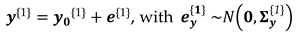
where are the vectors of geodetic measurements, the unknowable true quantity vectors of measurand, and the unknown vectors of measurement errors (note: the indices ‘1’ and ‘2’ inside the curly braces represent the quantities related to the first and second epoch in time, respectively).
By subtracting the Epoch 2 equation from the Epoch 1 equation, the univariate model can be formulated as a linear Gauss-Markov model, as follows:
with being the vector of the two-epoch geodetic observations differences, the unknown vector of errors of the two-epoch geodetic observations differences, the Jacobian matrix (also called the design matrix) of full rank , which in this case is a column vector of ones (i.e., ) , and the estimable unknown parameter, which in this case is a scalar that represents the unknown true difference between the two epochs. It is important to highlight that now our vector of observations corresponds to the differences of the geodetic measurements at two epochs in time. Furthermore, these differences are computed from the identical observations of each epoch.
After having defined the univariate model according to Eq. (2), we now need to resort to hypothesis testing theory to infer whether a subset of point fields measured in two epochs is stable/congruent or not. Typically, in displacement detection, the model under null hypothesis, denoted by , is set up for the case where all points to be analyzed are treated as stable points. In other words, the null hypothesis states that the null model in Eq. (2) explains the observations. Assuming normally distributed observation errors with expectation zero, i.e.:
the null hypothesis of the standard Gauss–Markov model in the linear form of the Eq. (2) is then given by:
 with the expectation operator, the dispersion operator, and the positive-definite variance matrix of . The variance matrix is obtained by applying the variance propagation law to the , which is the result of the sum of the variance matrices of the geodetic observations from Epoch 1 and Epoch 2 .
When the null model in Eq. (4) is assumed to be true, the scalar parameter can be estimated by simple least-squares calculus as:
and the estimated observation errors as being:
where is the known matrix of weights, taken as , where is the priori variance factor. The overall degrees of freedom (redundancy) of the model under is given by:
 where is the estimated variance matrix of the observation errors.
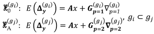
On the other hand, an alternative model can be proposed when there are doubts about the stability of points in the network. Here, we restrict ourselves – for simplicity of the analyses – measurements not contaminated by outliers. Thus, for the case of univariate approach, the model under the alternative hypothesis, denoted by , is to oppose Eq. (4) by an extended model that includes an extra parameter which describes the disturbance on the measurements in function of the displacement of a subset “” of network points, as follows:
 with being the matrix which captures the relationship between the displaced points and the changes in the measurements connected to them (hereafter, this matrix will be called displacement-design matrix). If the alternative model in Eq. (9) holds true, then the unknown parameters will be obtained as:
The redundancy of the model under is , with the estimated observation errors and estimated variance matrix of the observation errors under alternative hypothesis given respectively by:
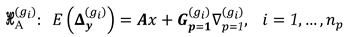
As a simple example, an alternative hypothesis may then be formulated for the case of having a specific point as displaced (), as can be seen in the illustration of a trilateration network in Figure 1. It is presumed that only point F has been moved to a new position F’. Consequently, this causes changes only to the observations connected to it. This means that such distances measured in the second epoch undergo deformations in the sense of stretching and/or compressing in relation to their initial states, whereas the other ones remain stable. The initial state refers to the first epoch the measurements were gathered, so that all network points are assumed to be free of displacements. For point F, for example, the matrix is described as:
The sign assigned to the elements of displacement-design matrix depends on the sign of the two-epoch geodetic observations differences. A positive sign means that at epoch 2 the measure was positively distorted and therefore the parameter acts positively (). The same occurs for the case in which the measure is reduced in relation to its initial state and, therefore, the parameter acts with a negative sign (). In this example (Figure 1), the shifted point F to its new position F’ makes the AF' segment smaller than its initial state AF. Consequently, the disturbance parameter on that measurement in function of the displacement of the F point acts with negative sign (). The same occurs for BF, i.e., BF' segment gets smaller than the BF segment (), while for the case of CF sign is positive, since CF' segment gets larger than CF ().
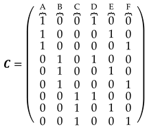
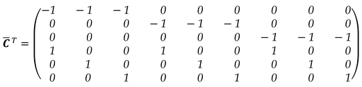
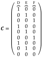
The displacement-design matrix in expression (10) has been constructed for the case of assuming only one single displaced point, which in our example was point F. In that case, the unknown parameter vector has become a scalar , and the displacement-design matrix has reduced to a unit vector, whose elements are exclusively formed by values of 0, 1 and -1, where 1 or -1 means that the ith parameter of magnitude or , respectively, affects the measurements connected to the point, and 0 means otherwise. However, as given by Eq. (9), we can design an overall displacement-design matrix , so that each column represents the displacement of a given point. For this, we first provide an auxiliary matrix which describes the general case of the relationship between the measures (matrix rows) and the network points (matrix columns), but without taking into account the sign of the unknown estimable vector . We call this matrix of Point-to-Measurement Connection Matrix, which for the network in Figure (1) is given by:
Then, the signs of the coefficients of the displacement-design matrix can be obtained generically from the application of a signum function as:
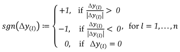 where is the sign function and gives a non-negativity value (absolute value) for each two-epoch geodetic observation differences. The result of Eq. (15) can be stacked into a vector as . Thus, the displacement-design matrix for the general case becomes:
where is the diagonalize operator which convert a vector to a diagonal matrix. Consequently, the alternative hypothesis is now given by:
where is the sign function and gives a non-negativity value (absolute value) for each two-epoch geodetic observation differences. The result of Eq. (15) can be stacked into a vector as . Thus, the displacement-design matrix for the general case becomes:
where is the diagonalize operator which convert a vector to a diagonal matrix. Consequently, the alternative hypothesis is now given by:

The displacement-design matrix can be developed in several ways, depending on which point, or group of points will be chosen to be monitored. Taking another example in Figure 2, if and , then a possible displacement-design matrix would be and for the case where the point A and B were considered simultaneously as displaced points. It is important to note that in this example the first and second columns of the matrix were selected, which refer to points A and B, respectively.
After postulating the null and alternative hypotheses, the test statistic derived from the concept of the maximum likelihood ratio test are computed as [37]:
Then, a test decision is then performed as

Under the null hypothesis , the test statistic follows the central chi-squared distribution with degrees of freedom; under the alternative hypothesis , the test statistic follows the non-central chi-squared distribution with degrees of freedom and non-centrality parameter . If the test statistic is larger than a critical value (), then a particular combination of tested points is flagged as displaced, where is the chi-squared critical value at a given significance level with degrees of freedom, i.e., . The probability level defines the size of a test and is often called the “false alarm probability”. Thus, the null model is assessed by specifying a significance level . [Note: the subscript "0" means that the test is performed for the case of having only one single alternative hypothesis. Thus, the non-centrality parameter and the significance level with the subscript "0" means that it is a single test involving only one single alternative hypothesis. In that case, rejecting the null hypothesis automatically consists of accepting the alternative hypothesis, and therefore, detection is the same as identification.]
In addition, the hypothesis test-based approach presented here is based on the mean-shift model: the alternative model is formulated under the condition that the displacement of the point (or a subset of network points) acts as a systematic effect by shifting the random error distribution under by its own value. This means that a displacement can cause a shift of the expectation under to a nonzero value. Therefore, hypothesis testing is often employed to check whether the possible shifting of the random error distribution under is, in fact, a systematic effect (bias) coming from a possible deformation or merely a random effect due to measurement uncertainties [38].
The alternative model in Eq. (17) has been formulated under the assumption that a specific group of points has undergone displacement. This group of points can be formulated for the cases where we have a single only one point displaced (Figure 1) or a subset of such points of the geodetic network (Figure 2). In other words, the number of points to be monitored and their locations on the network have been fully specified. This is a special case of testing the null hypothesis against only one single alternative hypothesis, and therefore, the rejection of the null model automatically implies the acceptance of the alternative model and vice versa.
3. Sequential Likelihood Ratio Tests for Unstable Points Identification – SLRTUPI
One of the questions that arises is how to define the number of points to be monitored and their locations. Clearly, geodesists need to work in an interdisciplinary way with other professional/areas so that an alternative model may be properly formulated [18]. However, even with such information, we may still have doubts whether there are points that a priori were assumed to be stable, whereas in fact they may be shifting. From a practical point of view, therefore, we often do not know well how many and which points are or are not stable. Here, all geodetic network points are subjected to be inspected, regardless of whether they are located on structure or not. Thus, a more conservative alternative hypothesis would be to assume that there is at least one point that is moving among all points involved in the geodetic network. Consequently, we would have alternative models for to be tested against the null hypothesis, i.e.:
 Note that represents the ith column vector of the displacement-design matrix . For the case of the network illustrated in Figure 1 and Figure 2, we would then have 6 alternative hypotheses, since we have a total of points, so that This means that we would have to test against , i.e.:
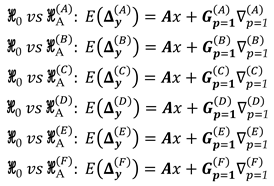
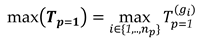
We are now dealing with testing involving multiple hypotheses. Now, we are interested in knowing which of the alternative hypotheses may lead to the rejection of the null hypothesis with a certain probability. To answer this, the test statistic in Eq. (18) is now computed for each of such tests , so that we would have a vector of test statistics, denoted by . In that case, the test statistic coming into effect is the maximum test value, which is computed as
The decision rule for this case is given by:
The decision rule in (23) states that if none of the tests get rejected, then we accept the null hypothesis . If the is larger than some percentile of its probability distribution (i.e., some critical value ), then there is evidence that there is a displaced point in the structure. In this case, we can only assume that detection occurred. The identification, however, is not straightforward. The identification (or localization) of the displaced point consists of seeking the point that produced the maximum test statistic , and whose value is greater than some critical value . Thus, point identification only happens when point detection necessarily exists, i.e., “point identification” only occurs when the null hypothesis is rejected. This means that the correct detection does not necessarily imply correct identification. For instance, we may correctly detect the occurrence of deformation, but wrongly identify a point as displaced, while in fact it is another point that has changed. The description of the success and failure rates will be covered in the next sections.
It is important to highlight that the maximum test statistic, now generally denoted by , is treated directly as a test statistic. Thus, the distribution of cannot be derived from well-known test distributions (e.g., Chi-squared distribution). Therefore, critical values cannot be taken from a statistical table but must be computed numerically. Here, the critical value is computed by Monte Carlo such that a user-defined Type I decision error rate “” for the proposed procedure is warranted [39]. In the next section, we provide details on how to compute the critical value for the proposed sequential procedure.
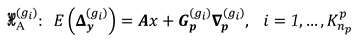
The procedure described so far allows only one single point to be identified. However, we may have multiple points displaced simultaneously. A more appropriate approach would be to apply a sequential test to decide the number and location of shifted points for the case where the null model is rejected. If the maximum test statistic value exceeds the critical value at the significance level adopted, i.e., if , the test statistics proceeds for (two possible unstable points). Since we do not know which group of two points might be shifting, we have to compute the test statistics by Eq. (18) from the possible combinations for two unstable points , and then identifying the corresponding candidate group for through the maximum value of the test statistic . Note that the extreme test statistic returns only one group of points or point. In general, the number of possible groups of points, denoted by , is given by:
For instance, for a geodetic network with points and by assuming two-point group to be tested, we would have a total of possible combinations. That would be the case for the geodetic network presented here, as can be seen either by Figure 1 or Figure 2, then we would have alternative models, i.e., . Note that for it is a particular case of having , as previously presented. Thus, the general cases of the alternative hypotheses can be expressed as:
 If the identified point with is also contained in the case of , i.e. if the one point flagged initially is among one of the pairs flagged subsequently, then the null hypothesis becomes specified according to the model identified at and the alternative hypothesis to the model defined at , as can be seen the example below:
 For example, if and the point A in the geodetic network illustrated in Figure 1 (or Figure 2) was identified by the , the model under the null hypothesis would become . If in the next step for , points A and C were identified by the , then the alternative hypothesis would be defined as . Note that is a subset of . To decide which of these models to select, we compute the test statistic based on the maximum likelihood ratio between and , denoted by [37]:
The result of Eq. (27) comes from the ratio between the maximum of the probability density function of under and , and the fact that the null hypothesis is (and must be) a subset of the alternative hypothesis. Thus, the selection of the most likely hypothesis is based on the following decision:
where and are the least-squares estimated observation errors for the model under the null and alternative hypothesis, respectively. For the example above, we would have for the null model and for the alternative one.
If the null hypothesis is not rejected, the testing ends and only the point corresponding to is flagged as unstable. On the other hand, if the null hypothesis is rejected again, then a new step is started by taking the model under the alternative hypothesis identified in the previous step as the null hypothesis. It proceeds by computing the test statistics for according to Eq. (18) for all possible combinations given by Eq. (24), identifying the corresponding candidate group for through the maximum value of the test statistic , and then checking if one of the points flagged in the previous step (i.e., for ) is among those flagged in the current step for . If this is the case, then the test is applied through Eq. (26) to decide between the null model defined by the identified model for and the alternative model for . This sequential procedure is repeated until any of the following conditions is met:
- (i)
- The current null hypothesis fails to be rejected.
- (ii)
- More than one group of geodetic network points is identified by the extreme statistic for a given , i.e., for the case where the hypotheses cannot be separable (statistical overlap), and therefore the identification cannot be accomplished.
- (iii)
- If the group of point(s) flagged by is not fully contained in the group of points flagged by , then the procedure ends with the null hypothesis given by the group of point(s) flagged by .
- (iv)
- Iteration reaches the threshold (i.e., until the maximum number of points to be evaluated is fully inspected). The definition of the maximum number of points will be detailed in the next section.
In general, therefore, the sequential testing procedure proposed here is based on likelihood ratio, which we now call Sequential Likelihood Ratio Tests for Unstable Points Identification (SLRTUPI). It consists in determining whether the additional subset of displaced point, considered in every new alternative hypothesis, is statistically significant or not, in terms of its impact on the quadratic form of the estimated observation errors, similar to its form for outlier detection [27]. Consequently, we can identify the number and the location of the displaced geodetic network points. Figure 3 provides step-by-step how to run the SLRTUPI procedure.
3.1. Monte Carlo Approach for Controlling the False Detection Rate
There is the probability of committing at least one false discovery, or Type I error when performing multiple hypotheses tests. Thus, Type I Error rate for the case where SLRTUPI is in play corresponds to the probability of incorrectly detecting at least one point as displaced while in fact there is none (i.e., accept at least one alternative hypothesis, when, in fact, the null hypothesis is true). This means that the SLRTUPI Type I decision error does not depend on all subsequent test steps, only on the extreme test statistic computed in its first step, i.e., only for in Eq. (22). The risk of rejecting a true is now one-fold: the undesired random event “reject a true ” can occur in any of the tests. Let the probability of rejecting a true in test be (the so-called “experimentwise error rate”) and let . Furthermore, assume the random events “reject a true in test ” to be approximately statistically independent. Then the total probability of rejecting a true in the multiple hypothesis test (the so-called “familywise error rate”, denoted here by ) is [11]:

The classical and well-known procedure to control the is to apply the Bonferroni equation by choosing [40]:
Unfortunately, the test statistics and consequently the random events “reject a true in test ” are statistically dependent. The extreme statistic captures such dependencies, as it is extracted from the . If such dependencies are neglected, then the computed critical values are erroneous, and the test decisions do not have the user-defined familywise error rate [34]. Here, the maximum test value in Equation (22) is treated directly as a test statistic [39]. Note that when using Equation (22) as a test statistic, the decision rule is based on a one-sided test of the form , as can be seen in expression (23). However, the distributions of cannot be derived from well-known test distributions (e.g., -distribution). Therefore, critical values cannot be taken from a statistical table but should be computed numerically. A rigorous computation of critical values requires a Monte Carlo technique.
The procedure to compute the critical values for is given step-by-step as follows:
- Generate a sequence of random vectors of the measurement errors for both epoch 1 and epoch 2 k = 1,..., m of the desired distribution. e.g.:where is known as the number of Monte Carlo experiments. In addition, Matlab's “mvnrnd” command may be used in this step, for example.
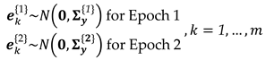
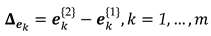
- For each pair and , k = 1,..., m compute the differences in errors between the two epochs, i.e.:
- Apply the least-squares to estimate the observation errors, as follows:where is known as the redundancy matrix, which is given by:
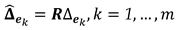 with the identity matrix.
 - Assemble the displacement-design matrix ,i = 1,..., np for each Monte Carlo experiment, according to equation (16), but the signs of the coefficients of the displacement-design matrix given by k = 1,..., m, and compute the test statistic by (18) and (22). The frequency distribution of approximates the probability distribution of .
- Sort in ascending order the , getting a sorted vector , such that:The sorted values in provide a discrete representation of the cumulative density function of the maximum test statistic .
- Determine the critical value :where denotes rounding down to next integer that indicates the position of the selected elements in the ascending order of . This position corresponds to a critical value for a stipulated overall false detection probability . This can be done for a sequence of values in parallel [34].
The Matlab function "kslrtupi.m" was elaborated for the computation of critical values. Inputs in the function are , where “” is the user-defined number of Monte Carlo experiments.
3.2. Determining the maximum possible number of points
Here, we objectively and universally demonstrate how to obtain the maximum number of points “” to be inspected by the SLRTUPI sequential procedure. The maximum number of points is also defined sequentially. The procedure to define the maximum number of points “” consists in finding a regular model (i.e., a matrix with full column rank) and, of course, that model has enough redundancy for the identification of unstable points. The step-by-step procedure to obtain the maximum possible number of points to be inspected by SLRTUPI is given by the flowchart in Figure 5.
If the full displacement-design matrix is specified by taking the total number of points in the network, i.e., by taking according to equation (16), then we fall into a problem in which there is a rank deficiency. Usually, the rank defect is greater than or equal to 1, because , where is the number of columns of the matrix . In this situation, the determinant of the normal matrix is zero. This means that such matrix cannot be considered invertible – the matrix is then said to be singular. Consequently, it is not possible to compute the test statistics by Equation (18). This demonstrates that .
By reducing the number of points by one unit, i.e., , we expect to find regular models (i.e., without rank deficiency). For that, it should be checked again whether there is rank defect or not. But now we have at our disposal not only one single group of points, but a combination of group of points. If at least one of the matrices presents rank defect, then must be reduced again by one unit, i.e., , and the rank computation is then repeated for group of points. If the rank defect persists, then the rank computation is repeated by decreasing to , otherwise we proceed to evaluate whether the test statistics computed in Equation (18) are different from each other. If there are at least two statistics with equal values, then a statistical overlap will be flagged. In that case, therefore, we should reduce to and restart the procedure. If the models are found to be regular and there is no statistical overlap, then the process ends with the value found.
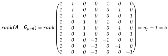
Important to highlight that the rank of the matrix depends on the behaviour of the signs of the coefficients of its displacement-design submatrix . The signs will also depend on the geometry of the geodetic network, as well as the unknown magnitude and number of points that have been shifted. Remember, however, captures these quantities. Although we have the limitation of computing the test statistics a priori, the procedure proposed above allows to determine the maximum number of testable points for identification. Generally, the choice of this maximum number is restricted to a subjective choice [11,13]. Here, Matlab function "pmax.m" was developed for the automatic computation of the maximum number of points. Inputs in the function are and , i.e., . Below are presented two possible scenarios that may occur in obtaining the for the geodetic network presented in the scope of this article (Figure 1).
Example 1:
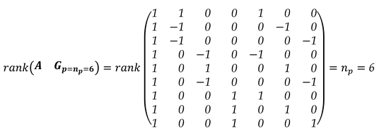 Note that the number of columns in the matrix (38) is but its . In that case, we would fall into a rank deficiency problem, because . If we considered that , then we would have group by Eq. (24), namely . However, in this case, the determinant of the normal matrix would be equal to zero, denoted by, which would characterize it as a singular matrix, and consequently would not allow the computation of the test statistics by the Eq. (18). By reducing to one unit (), we would have now a total of groups of 5 points, which would be the following: ; ; ; ; ; and . All these groups would now have full column rank with and . Thus, we would end and set .
However, another important analysis is needed. Although the determinants of the matrices constructed for each group of points are non-zero, their values are all equal to . Mostly, the test statistics computed for each of those groups by Eq. (18) would also have the same values. So, we would not be able to identify the group by the , since all the statistics are the same, i.e., there would be a statistical overlap. Consequently, we would only be able to get the information about displacement detection (i.e., ), but not identification. In order to have the possibility of identification, we would then decrease again to one unit (i.e., ), which would lead to a total of groups of 4 points. Now, the test statistics for each of would result of values different from each other, making identification possible. As a result, the maximum number of points to be considered would be for identification, which for that example we would get .
Example 2:
In this scenario, we would fall back into a problem where the matrix holds rank defect, but now with . If , we would have groups of 5 points to be considered, namely: ; ; and . Unfortunately, the rank of any of these groups would be equal to , and therefore we would still remain with rank deficiency problem. Moreover, the determinant of any normal matrix of these groups would be zero, i.e., . By reducing to one unit (i.e., ), we would have a total of groups of 4 points, but still with rank defect for the following groups: and As there would still be a lack of full column rank for some groups, we would again reduce . Now we would have a larger number of groups than the previous case, but of size equals to , i.e., groups of 3 points. In the latter case, however, we would still have only one single group of points that would cause a rank defect, namely . Again, we would proceed to decrease the maximum number of points followed by computing the rank of the matrices. Finally, we would find the maximum number of points, which in that case would be . All these groups of 2 points would have their respective matrices with full column rank and theirs test statistics would have different values from each other. Thus, would be the dimension found, so that all groups of 2 points would be testable for identification.
In addition to the examples given above, we may have cases where , which allows us to identify only one single point. In that case, the SLRTUPI procedure would not proceed in its sequential form, but would restrict only in its first step, i.e., only in the identification of a point by means of . And, if , then in that case we would have a situation in which it is not possible to detect displacements, since the network does not have enough redundancy for this purpose. This latter case may occur if the geodetic network is very poorly designed so that it will not be possible to detect displacements.
4. Results from computational simulation-based approach and real dataset: a trilateration geodetic network
4.1. Simulation setup
For a first performance testing of the SLRTUPI, we use a simulated trilateration network measured in two epochs (Figure 4), which is the same network presented in the previous sections (Figure 1 and Figure 2).
The network points are assumed to be stable at Epoch 1 (Table 1), so measurements connected to them are undisturbed (Table 2). In that case, the “true” distances for any segment formed by any two points and are easily computed as:

The true quantities in Table 2 are stacked into a vector as . To have simulated observations for Epoch 1 – see Equation 1 –, random errors are synthetically generated based on a multivariate normal distribution and added up to the true distances, as follows:
 The observations are assumed to be uncorrelated and with the same known standard deviation of , which is a value compatible with real cases. Then the main diagonal elements of the variance matrix for the Epoch 1 are the variances with values equal to , and its off-diagonal elements are zeros. Here, we use the Mersenne Twister algorithm to generate a sequence of random numbers and Box–Muller to transform it into a normal distribution [41,42]. For instance, Matlab's “mvnrnd” command can be applied to generate the random errors.
For Epoch 2, on the other hand, measurement distortions are simulated from the intentional displacement of the network points. The point displacements are simulated in terms of magnitude, denoted by , and orientation, denoted by , so that they can be propagate to the distance equation. To illustrate this step, consider that the segment formed by any two points and has suffered distortion when having point displaced to its new position (Figure 5). In this case, the true disturbance distance in Epoch 2 is computed as:
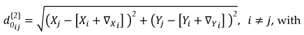
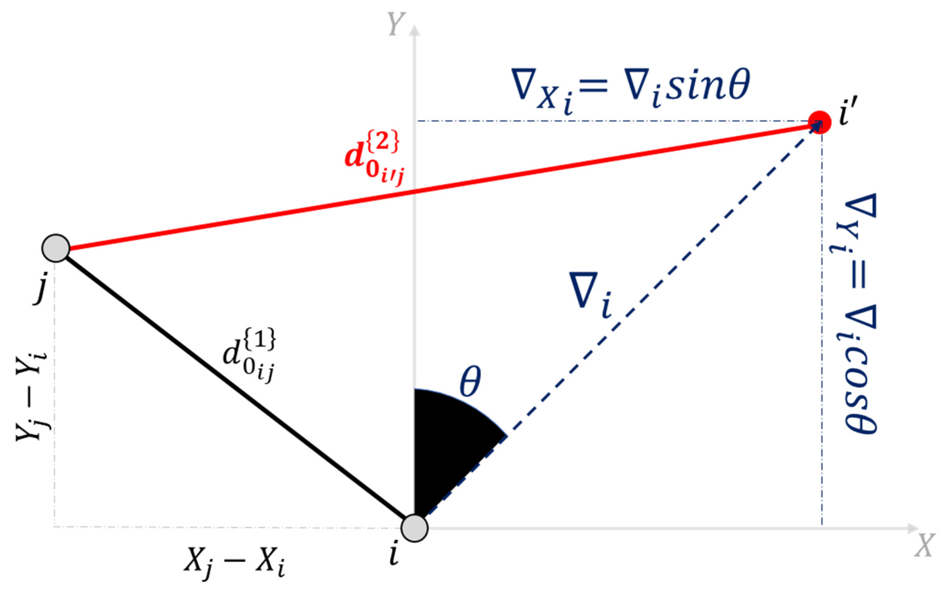
Figure 5.
Geometric aspect of simulating the displacement of a point and its effect on distance distortion.
Figure 5.
Geometric aspect of simulating the displacement of a point and its effect on distance distortion.
One can generalize the displacement simulation of any point or group of points from the Point-to-Measurement Connection Matrix (see Equation 14) from the following mathematical operations: first, we store the coordinates of the network points with no displacement into a vector . In our example, we have , which leads to:
Next, we use the Point-to-Measurement Connection Matrix in a modified form, denoted by , with the signs of its coefficients resulting from the orientation of the segment. For example, from point A towards point D, we would have with its corresponding components as and , and therefore, the first column of matrix would be . Following this reasoning, we would then have the general matrix in its transposed form for the case of the network in Figure 4 as
In general, therefore, we can simulate the disturbed distances in Epoch 2 by means the displacement of a point or groups of points from the relationship below:
where represents the Euclidean norm (also called the vector magnitude, Euclidean length, or 2-norm) of each column of a given matrix. In other words, this vector-wise 2-norm provides the distances of each segment of the network; and are the displacement vectors decomposed in the X and Y direction, which consist exclusively of elements with values of and for the selected group of points, respectively (see Equation 42), and 0 for points assumed to be free of displacements. The index “” in indicates a possible group, i.e., , as described in the previous section (see Equation 24). Note that the matrix composes the coordinates of the points with no displacements, whereas the second part of the Equation (45) represents the magnitude of the simulated displacements in the X-direction and Y-direction for a group of points .
For example, if we want to simulate the displacement of two points (i.e., ), then for the considered network we would have a total of groups, i.e., , namely: , , , , , , , , , , , , , and . To make it clearer, let's take the following specific example of having a simultaneous displacement of points A and D. i.e., for the group , with the following fixed definitions @ and @ , respectively. In that case, then we would have:
 Thus, the ‘true’ distances in Epoch 2 would be:
Next, the observations at the Epoch 2 are generated in the same way as it was done for Epoch 1 (see Equation 1), as follows:
Thus, the ‘true’ distances in Epoch 2 would be:
Next, the observations at the Epoch 2 are generated in the same way as it was done for Epoch 1 (see Equation 1), as follows:
The variance matrix for the Epoch 2 is taken to be the same as in Epoch 1, i.e., . Here, the value of is unimportant in this investigation. Now, we have all the necessary elements to apply SLRTUPI, as can be seen in the flowchart displayed in Figure 3. However, the simulation procedure explained so far is for only one single Monte Carlo experiment (i.e., ). Thus, a sequence of random observation vectors for both (Epoch 1) and (Epoch 2) are needed to evaluate the success and failure rates of the SLRTUPI. Here, therefore, we set up Monte Carlo experiments as suggest by [43], such that:

Remember that random vectors consist of the disturbed measurements due to the displacements. Displacements can vary in terms of their magnitude () and orientation () as well as the number of points (). Each scenario is simulated individually, i.e., we generate Monte Carlo experiments for each combination of (). Here, we evaluate for cases where the number of displaced points is and for the network in Figure 4.
The critical values were obtained for cases having the following significance levels: ; ; and , as displayed in Table 3.
These critical values were computed by 2 million of Monte Carlo experiments such that a user-defined Type I decision error for SLRTUPI was warranted (see topic 3.1.). To verify the consistency of these critical values found, we ran 200,000 Monte Carlo experiments under the condition of absent of displacements. In this case, the null hypothesis is fixed as true, and the detection of displacements represents the error of SLRTUPI in detecting displacements, when in fact they do not exist (false positives). Table 3 shows the significance level values found for these critical values, denoted by . The ones found must be as close as the ones setup (see the fourth column of the Table 3). Therefore, it is observed that the control of false positives was efficient by means of Monte Carlo Method, as described in Topic 3.1.
4.2. Numerical example for individually displaced points
In the first analysis, we have considered the case of having only one displaced point at a time. In that case, we had then 6 groups individually simulated, namely , with each group consisting of only one point, i.e.: . The magnitude of the displacement for each group was defined within the interval of [1,10] with increments of 1, where is the standard deviation of the observation, taken as – as mentioned before. The displacements were simulated to act in different orientations. The displacement orientation was simulated for the range of [0°,355°] with 5° increment. As a result, we had ten magnitudes of displacement for each of the 72 orientations, totalling 720 simulated displacements for each point (Figure 6).
200,000 Monte Carlo experiments were generated for each of those 720 cases, totalling 144 million trials for each point. It is important to remember that the simulated displacements of the points were converted to the space of the observations by Equation (45), which resulted in the corresponding disturbances on the measurements. Then, the Epoch 2 observations were generated from Equation (48), considering those true disturbance distances observations.
Finally, the probabilities levels associated with SLRTUPI (denoted by [.]) were computed as the ratio between the occurrence of a particular event – correct detection, wrong identification, overidentifications, statistical overlap or correct identification – and the number of possible cases (i.e., total number of Monte Carlo experiments 𝑚=200,000), which are given respectively by [38]:
where:
- – number of correct detections is the number of experiments in which SLRTUPI procedure correctly detect displacements. Inversely we have the missed detection rate for the case where SLRTUPI does not detect displacements, as follows:
- – number of wrong identifications is the number of experiments in which SLRTUPI flags only one single point as being unstable while the ‘true’ unstable point remains unidentified.
- – number of overidentifications positive is the number of experiments in which SLRTUPI identifies more than one point as being unstable, and among these points there is one that is correctly identified as unstable.
- – number of overidentifications negative is the number of experiments in which SLRTUPI identifies more than one point as being unstable, whereas the ‘true’ unstable point remains unidentified.
- – number of statistical overlaps is the number of experiments in which the detector flags two (or more) group of points simultaneously during a given iteration of SLRTUPI.
- – number of correct identifications is the number of experiments in which SLRTUPI correctly identifies the displaced point. In that case, we have the following relationship for the success rate of correct identification of the displaced point:
For identification to exist, detection must have occurred (see Equation 57). It is important to highlight that “displacement detection” only informs us whether or not there might have been at least one unstable point. For identification to exist, detection must have occurred. Detection does not guarantee correct identification, and it is clearly noted that identification is more difficult than detection (see Equation 58). This is explained in detail by Rofatto et al. [39]. Here it is also important to highlight that on average ~95% of the total experiments had ; no case occurred when ; ~3% had ; and ~2% had , according to the computation given by topic 3.2. Therefore, there were rare cases where .
Figure 7 shows the result of the correct identification. The black circles represent the radial range of magnitude displacements of 4mm, 1cm and 2cm. It is important to note that uncertainty of the two-epoch geodetic observations differences is . Therefore, these magnitudes of 4mm, 1cm and 2cm correspond to approximately , and .
Clearly, it is observed that the probability of correct identification depends on the geometry of the connections. Note that the highest success rates occur in the lines of sight. On the other hand, it is more difficult to identify in the directions perpendicular to the lines of sight, mainly for magnitudes close to the uncertainty of the measurement method . The increase in the significance level, and consequently a larger null hypothesis rejection region (smaller critical values) favours the identification of low magnitude displacements. On the other hand, higher significance levels reduce (slightly) the probability of correctly identifying displacements of larger magnitudes.
Figure 8 shows the result of the correct detection. Detection follows the same behaviour as identification in terms of the influence of the geometry of the point connections. There are no significant differences in terms of detection and identification for the case in which a low significance level is adopted ). The lower the critical value (higher significance level) the higher the detection rate.
Figure 9 provides the result for the wrong identification (also called Type III decision error). This decision error gets more expressive when the level is increased. In the worst case, we have for the case where point E moves and for . In general, the wrong identification occurs for large magnitudes in the region outside the lines of sight.
The overidentification class is presented in Figure 10. In general, such probability level become more evident when increasing . The overidentification was much rarer to occur, with its highest rate value of for . So, it is not shown here. On the other hand, the overidentification positive seems to occur more frequently than , especially close to the lines of sight and for large magnitudes.
Figure 11 portrays the behavior of the cumulative probability from the empirical cumulative distribution function (ECDF) of the identification and detection success when taking and for small (4mm), medium (1cm) and large (2cm) magnitude of displacement.
Increasing improved identification in the case of small (4mm) and medium (1cm) magnitude of displacement. Figure 11(a) reveals that approximately 90% () of the rates for achieved or less for (blue line); or less for (red line); or less for (yellow line); and or less for (purple line). In the case of medium magnitude of displacement (), approximately 90% () of the rates achieved or less for (blue line); or less for (red line); or less for (yellow line) and (purple line), as highlighted in Figure 11(b). The impact of the choice on the correct identification rate is not as critical for large magnitudes. Figure 11(c) shows that approximately 50% () of the rates for achieved or less for (blue line) and or less for (purple line). In that latter case, therefore, it is preferable to choose a lower familywise error ate to have higher identification success rate, i.e., . Detection always improves as the critical value increases, at the cost of having to increase false positive rates . In the next section, we present the testing performance of the SLRTUPI for the case of having 2 points displaced simultaneously.
4.3. Numerical example for simultaneously displaced points
In this second analysis, the scenarios were created for the case of having two points simultaneously unstable. For this, we have simulated all possible cases for at a time, i.e., we had then 15 groups of 2 points individually simulated . The magnitude of the displacement was fixed for each group as being of 10 . The displacement patterns of the two-point group varied in the same direction and opposite directions, as detailed in Figure 12. Table 4 and Table 5 display the results for correct identification and detection, respectively. [note: the results for each probability level are represented by , where max. and min. are the largest and smallest values].
In terms of detection and identification success rates, SLRTUPI depends on the interaction between the pattern in which the points move and the geometry of the geodetic network (Table 4 and Table 5). One geometry may be best for a given displacement pattern that one wish to monitor. The patterns (d), (e), (g) and (i) are the most difficult to identify for the case of the trilateration network considered in this work. This is due to the fact the displacements occur close to the perpendicular direction to the lines of sight (region more difficult to identify), as well as close to the direction where the Wrong Identification rate is larger, as also can be seen in the previous section for the case . On the other hand, displacement patterns with the pair of points displaced in different directions (c, f, j, k, and l in Figure 12) seem to be easier to identify. Furthermore, increasing the significance level does not always improve the identification rate of unstable points, but always improves detection (Table 5). In this scenario, we did not also have the occurrence of statistical overlap. The detection rate was very high (Table 5), so we can infer that it is very rare not to detect the displacement patterns simulated here.
4.4. Numerical example for simultaneously displaced points
In this last analysis under simulated conditions, the scenarios were created for the case of having three points simultaneously simulated as unstable. For this, we have simulated all possible cases for at a time, i.e., we had then 20 groups of 3 points individually simulated . The magnitude of the displacement was also fixed for each group as being of 10 . The displacement patterns of the three-point group varied in the same direction and opposite directions, as detailed in Figure 13. Table 6 and Table 7 display the results for correct identification and detection for the case of having three mutually displaced points , respectively.
The identification for the case where we have 3 simultaneous displacements is more difficult than the case of 2 simultaneous displacements (see Table 4 and Table 6), but the correct detection rates are similar (see Table 5 and Table 7). In fact, most of the patterns simulated here for are difficult to identify. The pattern described in (c, k, and l) are the easiest to identify (Table 6).
The numerical examples described here provide a way in which the user may design the geodetic network as best as possible to find the optimum geometry to identify a certain type of displacement pattern. In the next section, we will evaluate the performance of SLRTUPI for simulations of real displacements in the field.
4.4. Real example
In this experiment, the geodetic network described in Figure 4 was materialized in the field. For this, the distances were obtained using the total station FOIF OTS 685, with linear uncertainty of 2mm + 2ppm (manufacturer specifications). Tribrach were used for both the Total Station and the Reflector Prisms. The supplement files are provided for those interested in the dataset for reproducing the experiments or even for testing other procedures. Epoch 1 was recorded as no displacements, while Epoch 2 various patterns were tested. For this, the displacements at the points were intentionally applied radially. Points A, B and C were kept fixed, i.e., they were not subjected to displacement, whereas D, E and F were considered the points to be monitored. The displacements were performed in the field, by moving the reflector 1 cm from the initial position (Epoch 1) to the new positions (Epoch 2), as indicated in Figure 14. Four cases were tested for shifting only one point at a time, as displayed in Figure 14(a,b,c,d); three scenarios for 2 and 3 simultaneous displacements, with the patterns shown in Figure 14(e,f,g) and Figure 14(h,i,j), respectively, totalling 23 experiments (12 for ; 8 for ; and 3 ).
First, SLRTUPI was applied under the condition that all points are unstable, which in that case Point-to-Measurement Connection Matrix is the one given in (14). Based on the simulated results, we adopted a significance level of , which resulted in a critical value of . The results are very promising, as can be seen in Table 8. We had a success rate in identification of ~74%, and the correct detection rate was 100% for all scenarios.
The results show that of the 23 experiments, only 6 wrong identifications occurred. Most experiments resulted in , with a few exceptions, such as: [D, E, F] in Figure 15h resulted , consequently the wrong identification was already expected; and [D, E, F] in Figure 15i resulted .
Here, we also apply SLRTUPI based on the a priori knowledge that points A, B and C are known to be stable. In the latter, therefore, the matrix in (14) was reduced to:
Because we had a change in the mathematical model in terms of redundancy – 3 points less to be monitored than the previous case, consequently there was better redundancy than monitoring all points –, the critical value found was = 6.64 for = 10%. As a result, the correct identification rates increased from ~74% to ~96% when points A, B and C were fixed (adopted as control points), as can be seen in Table 9. We had only one single case of Type III Error among the 23 experiments. This is due to the fact of increasing redundancy, since we have gone from 6 points to 3 points to be monitored for the same set of observations. Furthermore, = 3 for all experiments where A, B, C were taken as fixed.
Finally, SLRTUPI was applied under a scenario in which there are no displacements to verify the efficiency of the Type I Error control (specifically, of the familywise error rate ). For this, new measurements were performed and stamped to Epoch 2, but now without applying any intentional displacement to the points. As a result, no displacement was detected in the field experiments, which shows that SLRTUPI can guarantee user-defined Type I Error control under real conditions of use.
5. Contributions
In this contribution, we present a statistical method for detecting and identifying unstable points for geodetic deformation analysis, namely Sequential Likelihood Ratio Test for Unstable Points Identification (SLRTUPI). The method makes use of the differences of measurements taken at two epochs in time instead of using the classic difference of estimated coordinates. As an advantage, we will always have a linear model, and therefore the model nonlinearity problem does not affect the test power. In addition, another advantage is to avoid the S-transformation to maintain the same datum between epochs.
The method is not restricted to points subject to monitoring but is applied in such a way that all points participate in its inspection. However, the power of the identification improves considerably if we know in advance which points are stable (see Table 8 and Table 9). The results support that the success of the proposed method depends on the interaction between the displacement pattern and the network geometry. In the case of the trilateration network used as a case study in this contribution, we observe that for the case of having only one single point displaced, the highest success rates occur in the lines of sight (Figure 7 and Figure 8). When more than one point is unstable simultaneously, success rates are generally higher for the scenarios where the displacements occur in opposite directions (see Table 4, Table 5, Table 6 and Table 7). More experiments based on different types of geodetic networks (such as, levelling and GNSS networks) will be conducted in the future works.
The larger the number of points displaced simultaneously, the more difficult the identification. However, success rates depend on the geometry and redundancy of the network. Furthermore, detection is always larger than identification. Although identification is important to localize displacement, detection plays a dominant role for the activities that involves risk assessment, such as the deformation analysis. It is preferable that detection occurs even if identification does not occur in the expected way. It is crucial that a system raises an alarm when displacements are detected, even though their location may be wrong. In this sense, we also observe that increasing the significance level does not always improve the identification rate, but always improves detection.
It is important to highlight here that the false positive rates (Type I errors) are efficiently controlled from the definition of the familywise error rate by the user (). The approach for controlling that decision error is based on Monte Carlo. Of course, this requires some computational cost, but nothing prohibitive. One way to save computational costs would be to develop a methodology based on artificial neural networks, as done for example by [44], or some other alternatives, such as [45]. This will be investigated in future work.
Another important contribution is that now the maximum number of points to be inspected by the SLRTUPI procedure is not based on non-objective choices, but rather determined from the rank analysis of the design matrices involved and the occurrence of statistical overlap. Consequently, the method avoids the occurrence of statistical overlap, which is common in multiple test problems [39,45]. More experiments will be needed to understand the effect of determining on the detection and identification of unstable points.
The simulation methodology described here can also be applied in the design stage of a geodetic network for deformation analysis purposes. This allows the user to know a priori how the measurement system (in this case, the geodetic network) should be optimally designed so that it is able to detect and/or identify a certain displacement pattern for a given probability. As a result, reliability measures can be easily extracted, such as Minimal Identifiable Displacement (MID) and Minimal Detectable Displacement (MDD) from its corresponding success rates and by a given user-defined significance level . More experiments for different geodetic networks will be needed to evaluate the ability of the measurement system to identify possible outliers (internal reliability) and the effect of these undetected errors on the quality of deformation analysis results (external reliability).
In future works we will also evaluate the question of formulating the null hypothesis with parameter-free, so that the differences between the measurements in the two epochs may be taken as being directly the errors. Thus, the test could be simpler, with the benefit that the degrees of freedom of the test will be larger than the model adopted here.
Finally, it is emphasized that the proposed method can be extended to the outlier detection problem. The proposed method can also be extended to the case of Point Clouds from Terrestrial Laser Scanning in case of having to decide between the different models of surface representation in the area-based deformation analyses problems. The dataset and algorithms used in this work are available for those interested in reproducing the results and/or applying them to other methodologies, as follows: https://data.mendeley.com/datasets/msg783rh2y/draft?a=607de244-7c1d-417f-a9c8-81281d8a6056
Conflicts of Interest
The authors declare no conflicts of interest.
References
- Welsch WM, Heunecke O. Models and terminology for the analysis of geodetic monitoring observations. (2001). In: Official report of the ad-hoc committee of FIG working group 6.1. X FIG international symposium on deformation measurements. Figure Publication No. 25, ISSN 87-90907-10-8. Retrieved from https://www.fig.net/resources/publications/figpub/pub25/figpub25.asp.
- Pelzer H (1971) Zur Analyse geodätischer Deformationsmessungen, Ph.D. Thesis (in German). Deutsche Geodätische Kommission, Reihe C: Dissertationen - Heft Nr. 164, München, Germany.
- van Mierlo J (1978) A testing procedure for analysing geodetic deformation measurements. In: Proceedings of the II. International symposium of deformation measurements by geodetic methods. Bonn, Germany, September 25–28, 1978, Konrad Wittwer, Stuttgart, pp 321–353.
- Niemeier W (1981). Statistical tests for detecting movements in repeatedly measured geodetic networks. In: P. Vyskočil, R. Green and H. Mälzer (Editors), Recent Crustal Movements, 1979. Tectonophysics, 71: 335–351. [CrossRef]
- Caspary WF (2000) Concepts of network and deformation analysis. The University of New South Wales, Kensington.
- Niemeier W (2008) Ausgleichungsrechnung, statistische auswertemethoden, 2nd edn. de Gruyter, Berlin.
- Heunecke O, Kuhlmann H, Welsch WM, Eichhorn A, Neuner H (2013) Handbuch Ingenieurgeodäsie: Auswertung geodätischer Überwachungsmessungen. 2nd edn., Wichmann, Heidelberg.
- Chen YQ (1983) Analysis of deformation surveys—a generalized method. Technical Report No. 94. University of New Brunswick. Fredericton.
- Nowel K, Kamiński W (2014) Robust estimation of deformation from observation differences for free control networks. J Geod 88(8):749–764. [CrossRef]
- Nowel K (2015) Robust M-estimation in analysis of control network deformations: classical and new method. J Surv Eng 141(4):04015002. [CrossRef]
- Lehmann, Rüdiger and Lösler, Michael. "Congruence analysis of geodetic networks – hypothesis tests versus model selection by information criteria" Journal of Applied Geodesy, vol. 11, no. 4, 2017, pp. 271-283. [CrossRef]
- Baarda W (1968) A testing procedure for use in geodetic networks, Vol. 2, Number 5, Netherlands Geodetic Commission, Publication on Geodesy, Delft, Netherlands. Retrieve from http://www.ncgeo.nl/phocadownload/09Baarda.pdf.
- Nowel, K. Specification of deformation congruence models using combinatorial iterative DIA testing procedure. J Geod 94, 118 (2020). [CrossRef]
- Hekimoglu S, Erdogan B, Butterworth S (2010) Increasing the efficacy of the conventional deformation analysis methods: alternative strategy. J Surv Eng 136(2):53–62. [CrossRef]
- Erdogan B, Hekimoglu S (2014) Effect of subnetwork configuration design on deformation analysis. Surv Rev 46(335):142–148. [CrossRef]
- Durdag UM, Hekimoglu S, Erdogan B (2018) Reliability of models in kinematic deformation analysis. J Surv Eng 144(3):04018004. [CrossRef]
- Velsink, H. On the deformation analysis of point fields. J Geod 89, 1071–1087 (2015). [CrossRef]
- Velsink H (2018) Testing methods for adjustment models with constraints. J Surv Eng 144(4):04018009. [CrossRef]
- Baselga S (2011) Exhaustive search procedure for multiple outlier detection. Acta Geod Geophys Hung 46(4):401–416. [CrossRef]
- Biagi L, Caldera S (2013) An efficient leave one block out approach to identify outliers. J Appl Geod 7(1):11–19. [CrossRef]
- Wujanz D, Krueger D, Neitzel F (2016) Identification of stable areas in unreferenced laser scans for deformation measurement. Photogram Rec 31(155):261–280. [CrossRef]
- Zienkiewicz M H (2014) Application of Msplit estimation to determine control points displacements in networks with an unstable reference system. Surv Rev 47(342):174–180. [CrossRef]
- Zienkiewicz M H, Baryla R (2015) Determination of vertical indicators of ground deformation in the old and main city of Gdansk area by applying unconventional method of robust estimation. Acta Geodyn Geomater 12(3):249–257. [CrossRef]
- Wiśniewski Z, ZienkiewiczMH(2016) Shift-M* split estimation in deformation analyses. J Surv Eng 142(4):1–13. [CrossRef]
- Duchnowski R (2010) Median-based estimates and their application in controlling reference mark stability. J Surv Eng 136(2):47–52. [CrossRef]
- Duchnowski R (2013) Hodges-Lehmann estimates in deformation analyses. J Geod 87(10–12):873–884. [CrossRef]
- I. Klein, M. T. Matsuoka, M. P. Guzatto & F. G. Nievinski (2017) An approach to identify multiple outliers based on sequential likelihood ratio tests, Survey Review, 49:357, 449-457. [CrossRef]
- Lazzarini T, Laudyn I, Chrzanowski A, Ga´zdzicki J, Janusz W, Wiłun Z, Mayzel B, Mikucki Z (1977) Geodetic measurements of displacements of structures and their surroundings. PPWK, Warsaw (in Polish).
- Chrzanowski A, Chen YQ (1990) Deformation monitoring, analysis and prediction-status report FIG XIX international congress. Helsinki 6(604.1):83–97.
- Baarda W., 1973. S-Transformation and Criterion Matrices. Publications on Geodesy, New Series, Vol. 5, No. 1, Netherland Geodetic Commission, Delft, The Netherlands.
- Nowel K (2019) Squared Msplit(q) S-transformation of control network deformations. J Geod 93:1025–1044. [CrossRef]
- Erdogan B., Hekimoglu S., Durdag U M. A new univariate deformation analysis approach considering displacements as model errors. Stud. Geophys. Geod., 65 (2021), 1-14. [CrossRef]
- Aydin C (2017) Effects of displaced reference points on deformation analysis. J Surv Eng 143(3):1–8. [CrossRef]
- Hekimoglu S, Erdogan B, Soycan M, Durdag U M (2014). Univariate Approach for Detecting Outliers in Geodetic Networks. J Surv Eng 140(2):1–8. [CrossRef]
- Lehmann, R. and Lösler, M. "Hypothesis Testing in Non-Linear Models Exemplified by the Planar Coordinate Transformations" Journal of Geodetic Science, vol. 8, no. 1, 2018, pp. 98-114. [CrossRef]
- Lehmann R (2012) Improved critical values for extreme normalized and studentized residuals in Gauss–Markov models. J Geod (86)12: 1137 – 1146. [CrossRef]
- Teunissen PJG (2000) Testing theory: an introduction. Series on mathematical geodesy and positioning. Delft University Press, Delft.
- Lehmann, R. On the formulation of the alternative hypothesis for geodetic outlier detection. J Geod 87, 373–386 (2013). [CrossRef]
- Rofatto VF, Matsuoka MT, Klein I, Roberto Veronez M, da Silveira LG Jr. A Monte Carlo-Based Outlier Diagnosis Method for Sensitivity Analysis. Remote Sensing. 2020; 12(5):860.
- Abdi H (2007) The Bonferonni and Šidák corrections for multiple comparisons. In: Neil Salkind (ed) Encyclopedia of measurement and statistics. Sage, Thousand Oaks.
- Matsumoto, M.; Nishimura, T. Mersenne twister: A 623-dimensionally equidistributed uniform pseudo-random number generator. ACM Trans. Model. Comput. Simul. 1998, 8, 3–30. [CrossRef]
- Box, G.E.P.; Muller, M.E. A Note on the Generation of Random Normal Deviates. Ann. Math. Stat. 1958, 29, 610–611. [CrossRef]
- Vinicius Francisco Rofatto, M. T. Matsuoka, I. Klein, M. R. Veronez, M. L. Bonimani & R. Lehmann (2020) A half-century of Baarda’s concept of reliability: a review, new perspectives, and applications, Survey Review, 52:372, 261-277. [CrossRef]
- Vinicius Francisco Rofatto, Marcelo Tomio Matsuoka, Ivandro Klein, Maria Luísa Silva Bonimani, Bruno Póvoa Rodrigues, Caio Cesar de Campos, Mauricio Roberto Veronez & Luiz Gonzaga da Silveira Jr. (2022) An artificial neural network-based critical values for multiple hypothesis testing: data-snooping case, Survey Review, 54:386, 440-455. [CrossRef]
- Lehmann R, Lösler M (2016) Multiple Outlier Detection: Hypothesis Tests Versus Model Selection by Information Criteria. J Surv Eng, 142(4). [CrossRef]
- Zaminpardaz, S., Teunissen, P.J.G. DIA-datasnooping and identifiability. J Geod 93, 85–101 (2019). [CrossRef]
Figure 1.
Horizontal trilateration network deformed due to the displacement (step) of point F to a new position F’.
Figure 1.
Horizontal trilateration network deformed due to the displacement (step) of point F to a new position F’.
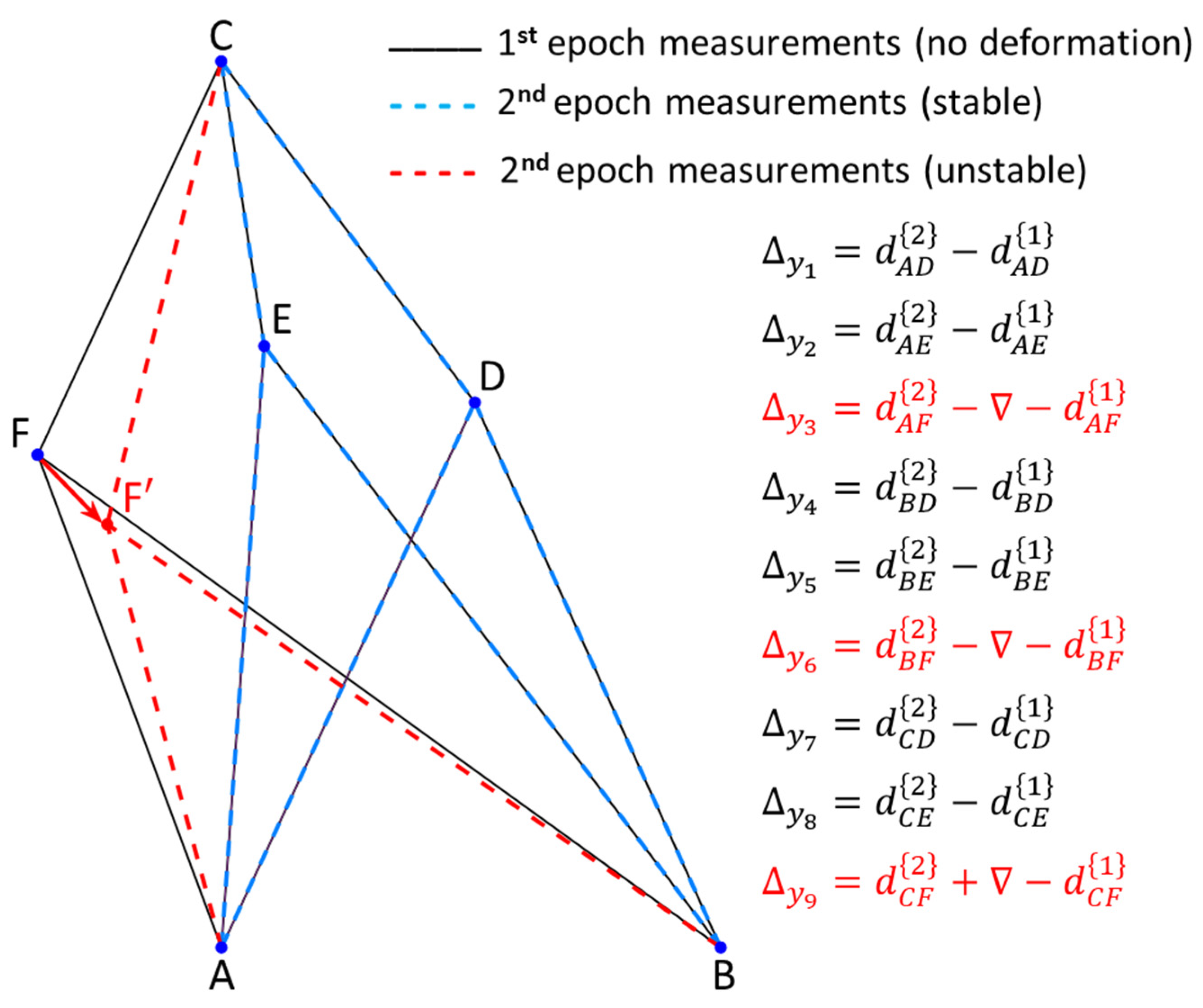
Figure 2.
Horizontal trilateration network deformed due to the simultaneous displacement (step) of point A to a new position A’ and B to B’.
Figure 2.
Horizontal trilateration network deformed due to the simultaneous displacement (step) of point A to a new position A’ and B to B’.
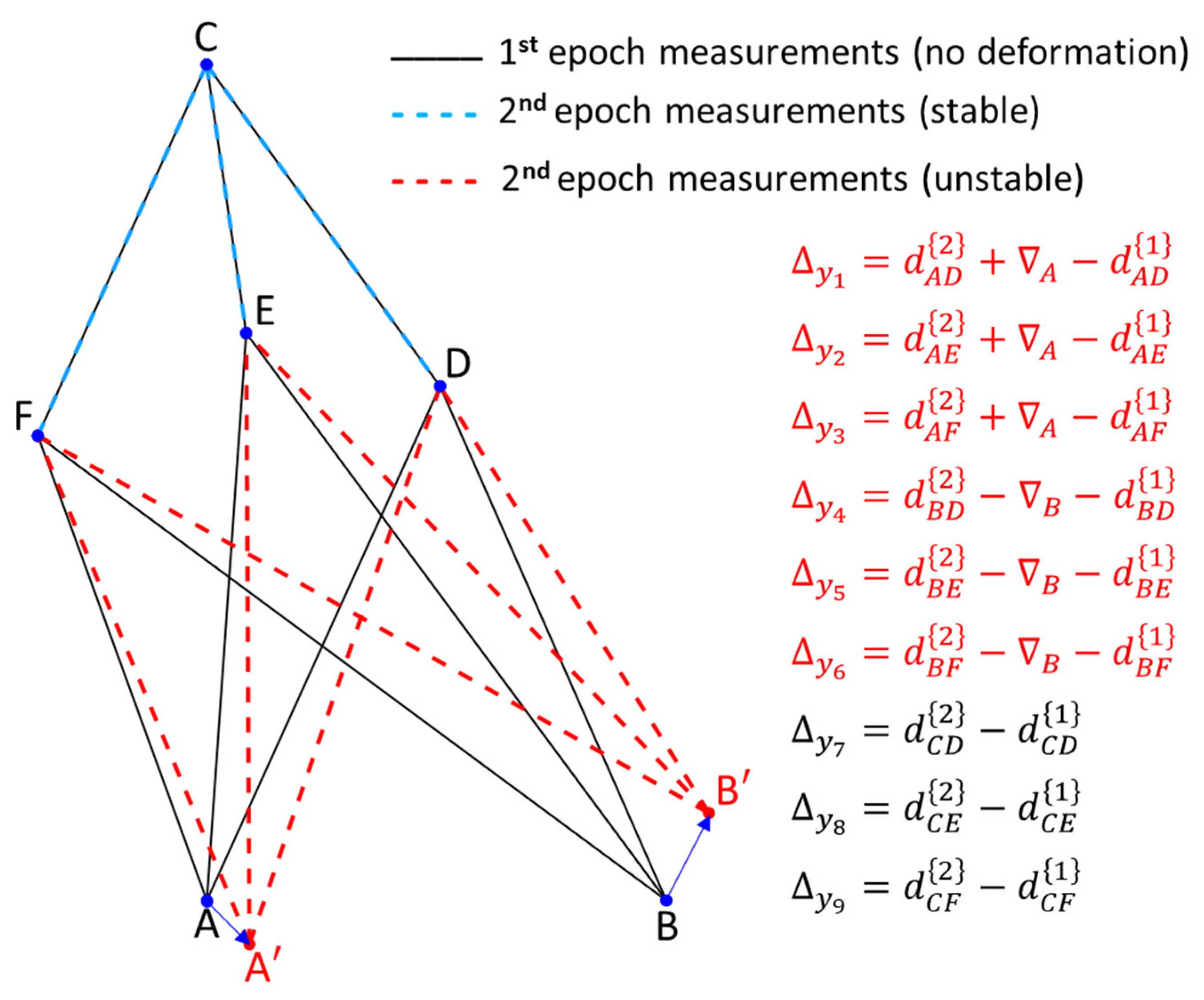
Figure 3.
Flowchart of the SLRTUPI.
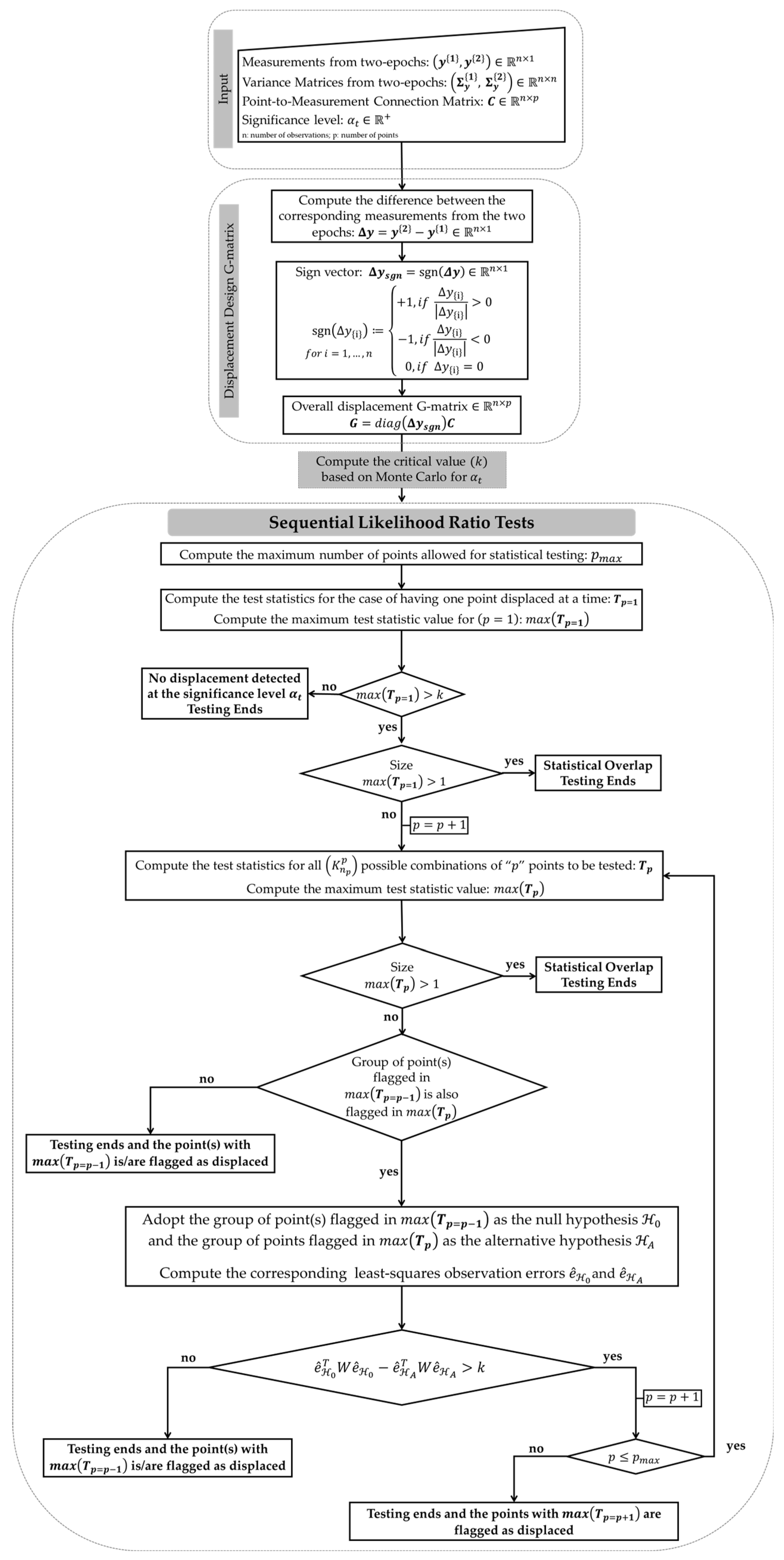
Figure 5.
Flowchart for determining the maximum possible number of points to be inspected by SLTUPI.
Figure 5.
Flowchart for determining the maximum possible number of points to be inspected by SLTUPI.
Figure 4.
Simulated Trilateration Network.
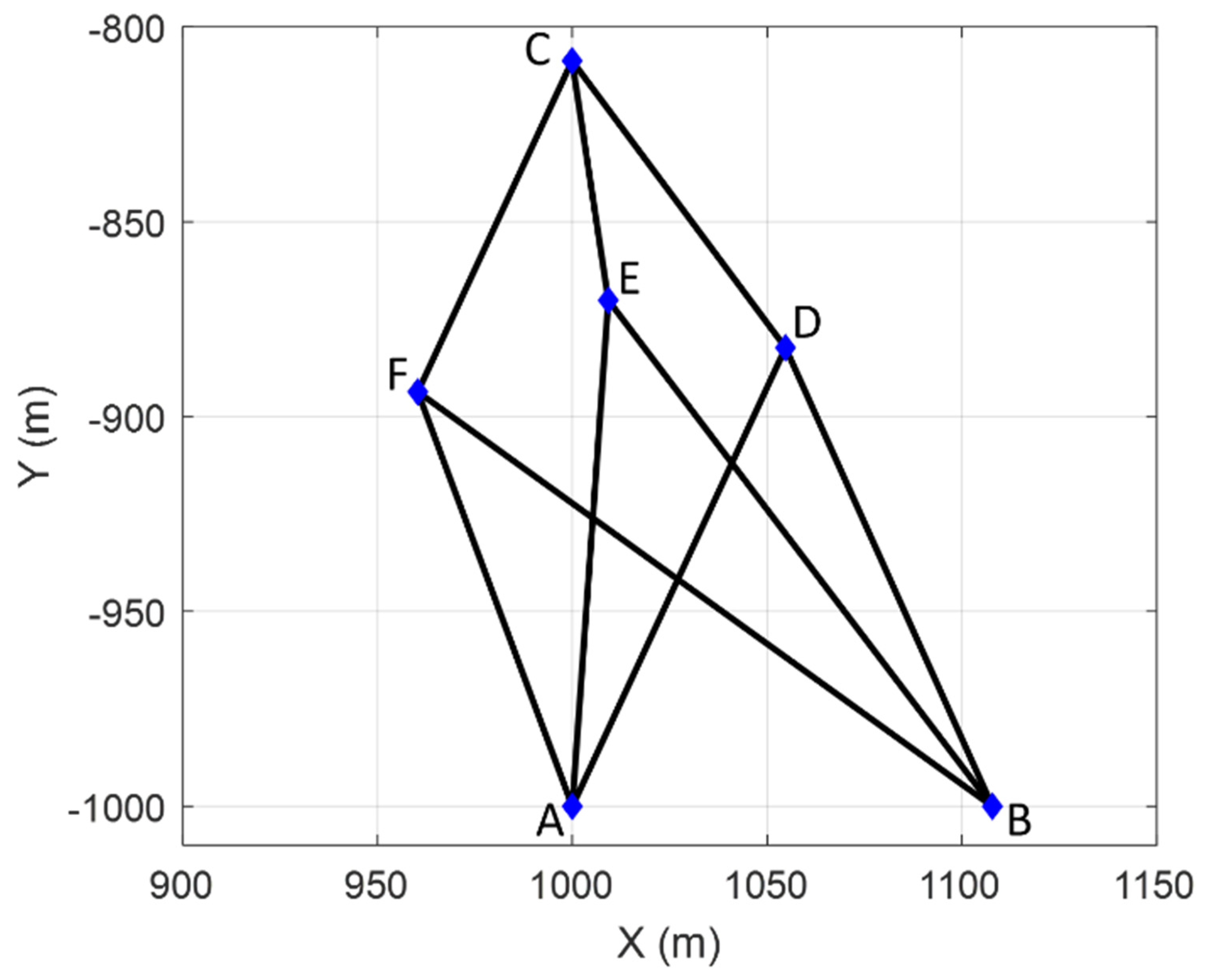
Figure 6.
Simulated displacements for each point (case ).
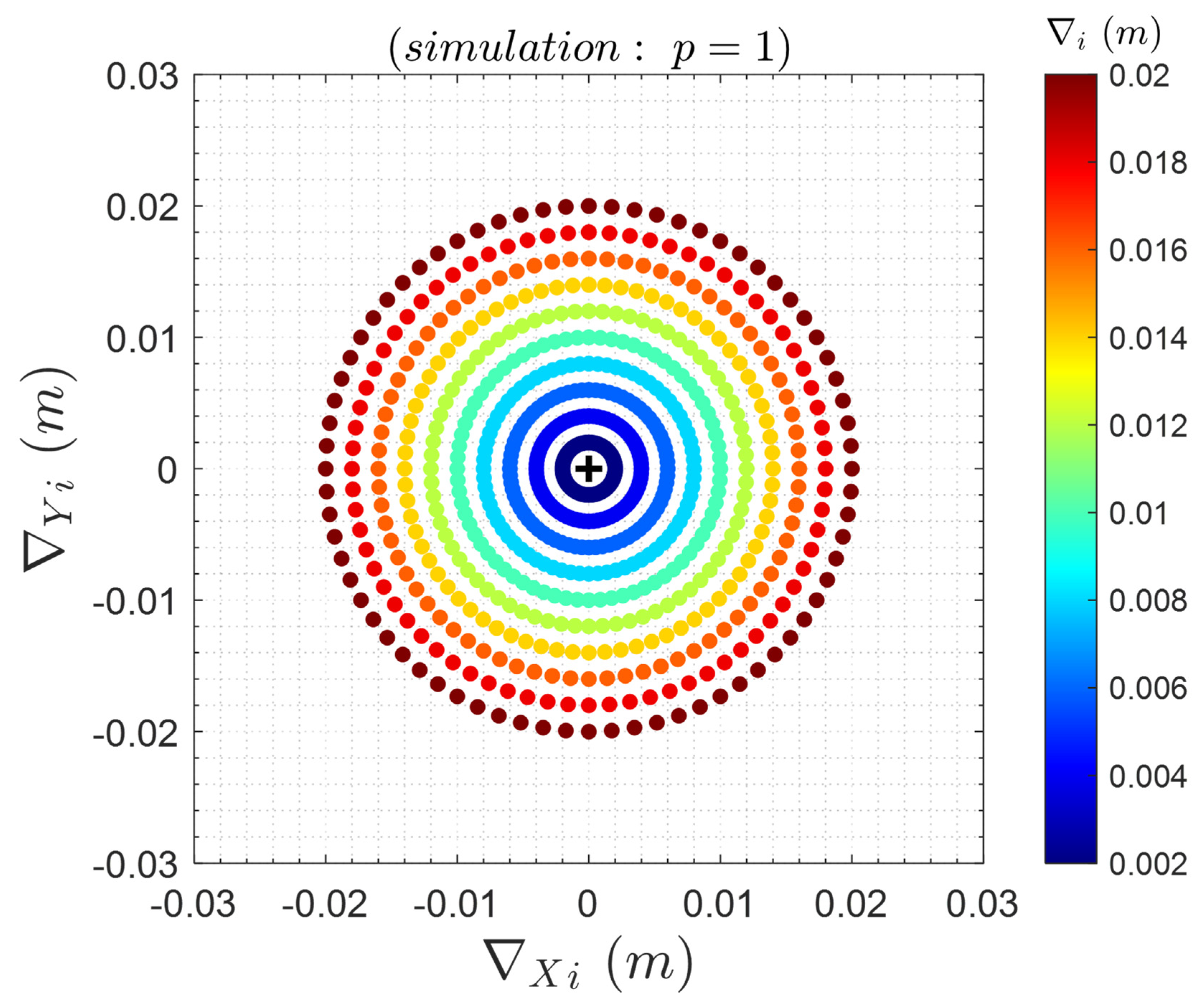
Figure 7.
Probability of correct identification (): (a) for ; (b) for ; (c) for ; and (d) for .
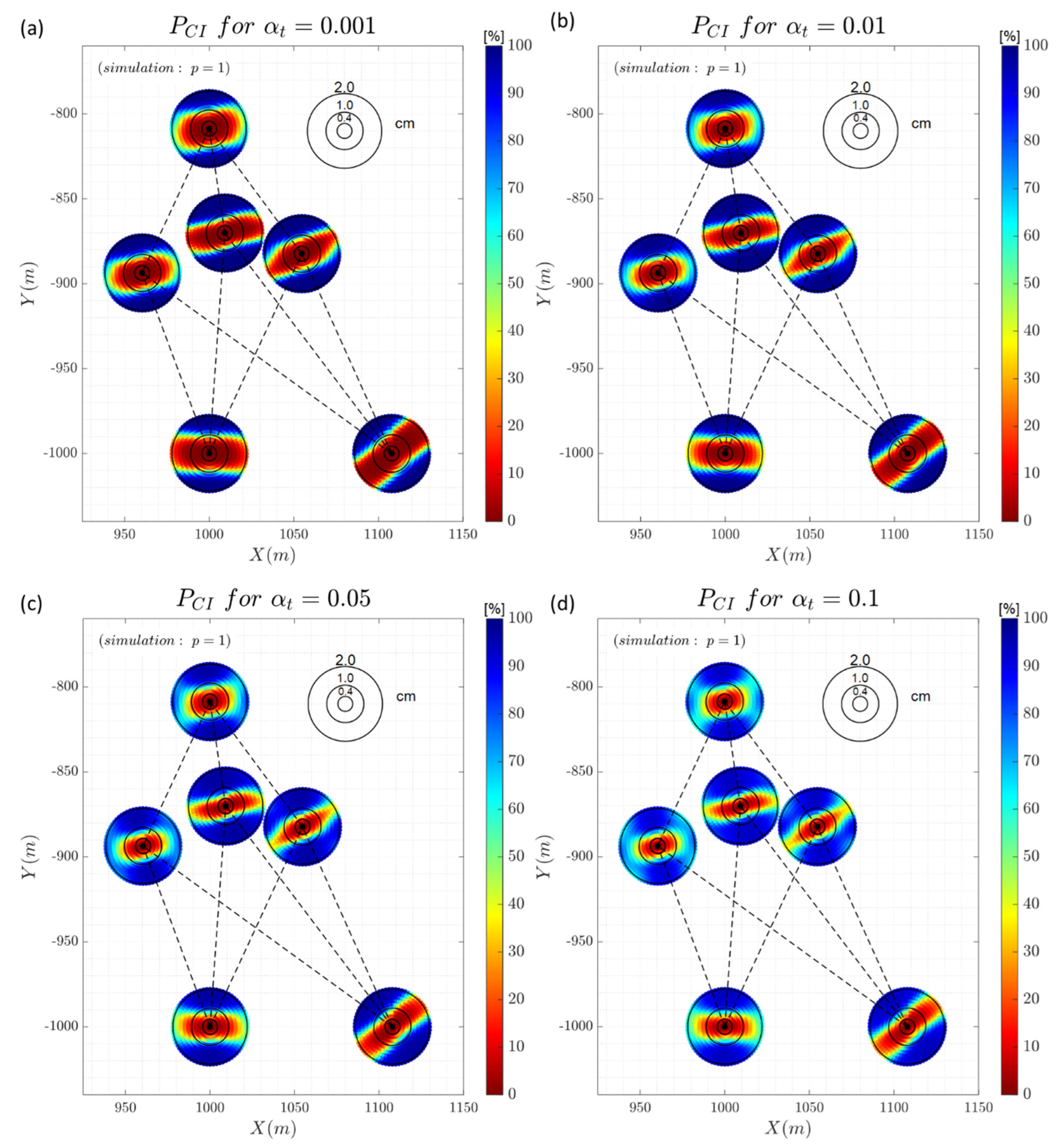
Figure 8.
Probability of correct detection (): (a) for ; (b) for ; (c) for ; and (d) for .
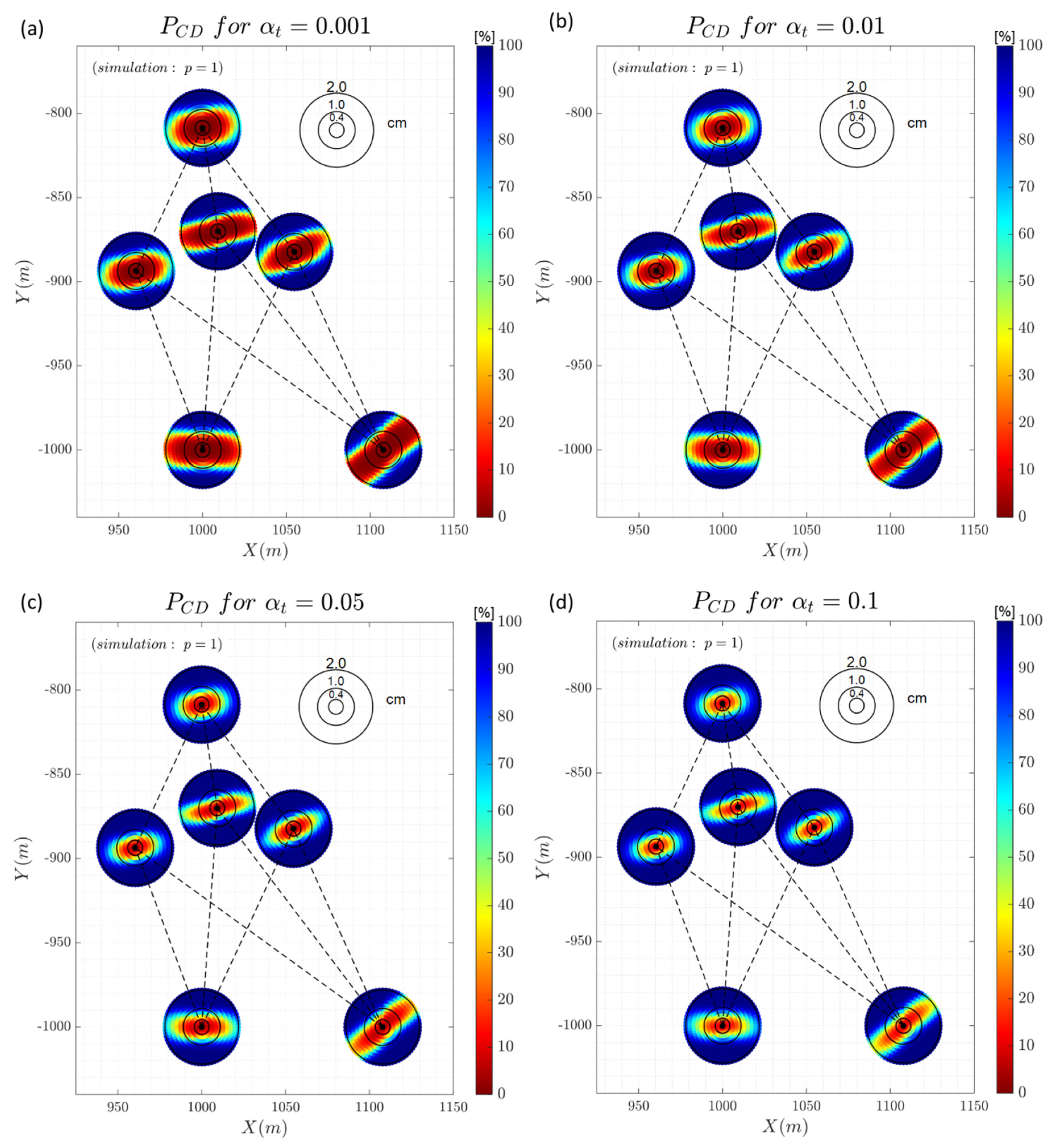
Figure 9.
Probability of wrong identification (): (a) for ; (b) for ; (c) for ; and (d) for .
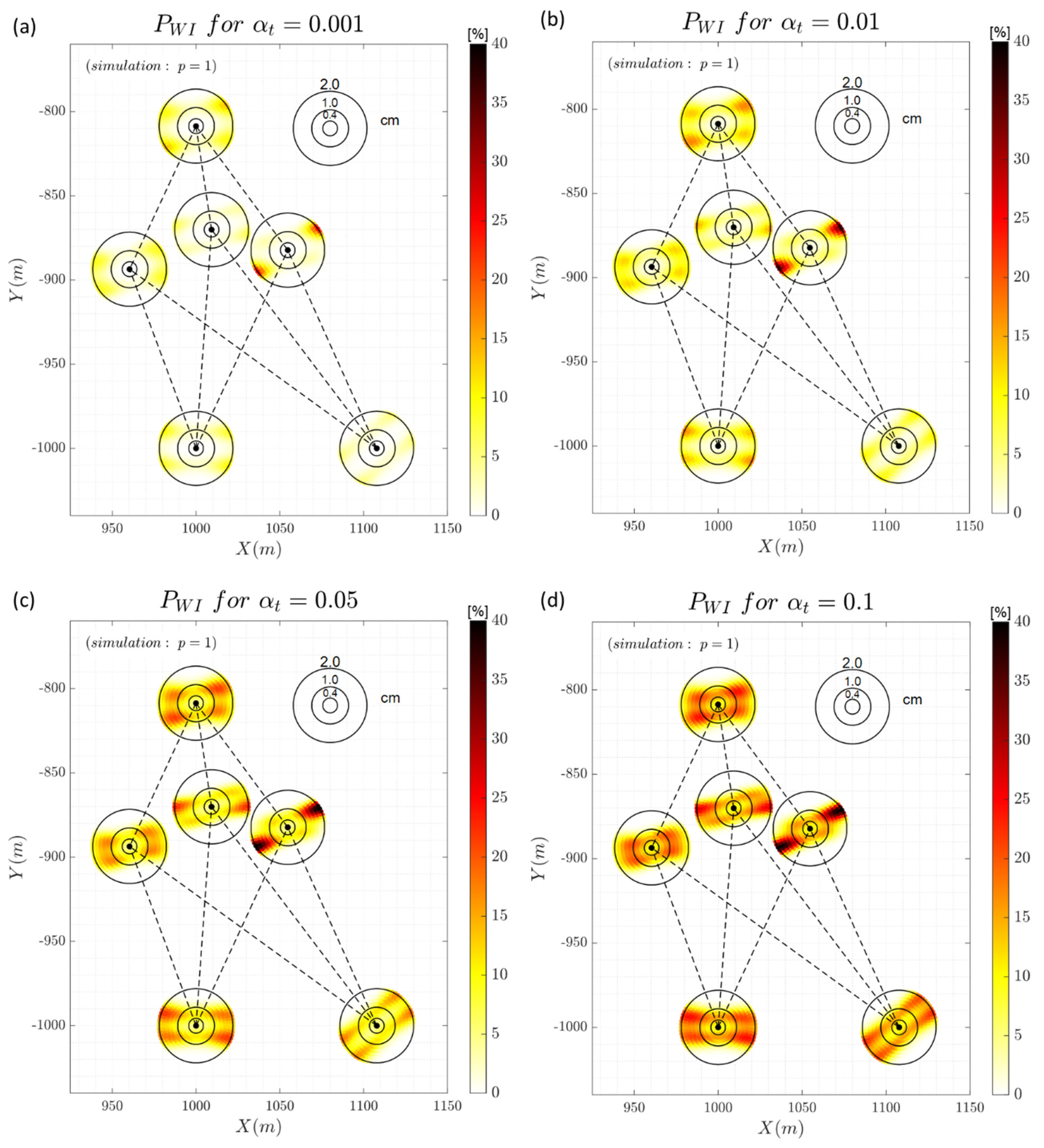
Figure 10.
Probability of overidentification for the case where SLRTUPI identifies the displaced point and others (): (a) for ; (b) for ; (c) for ; and (d) for .
Figure 10.
Probability of overidentification for the case where SLRTUPI identifies the displaced point and others (): (a) for ; (b) for ; (c) for ; and (d) for .
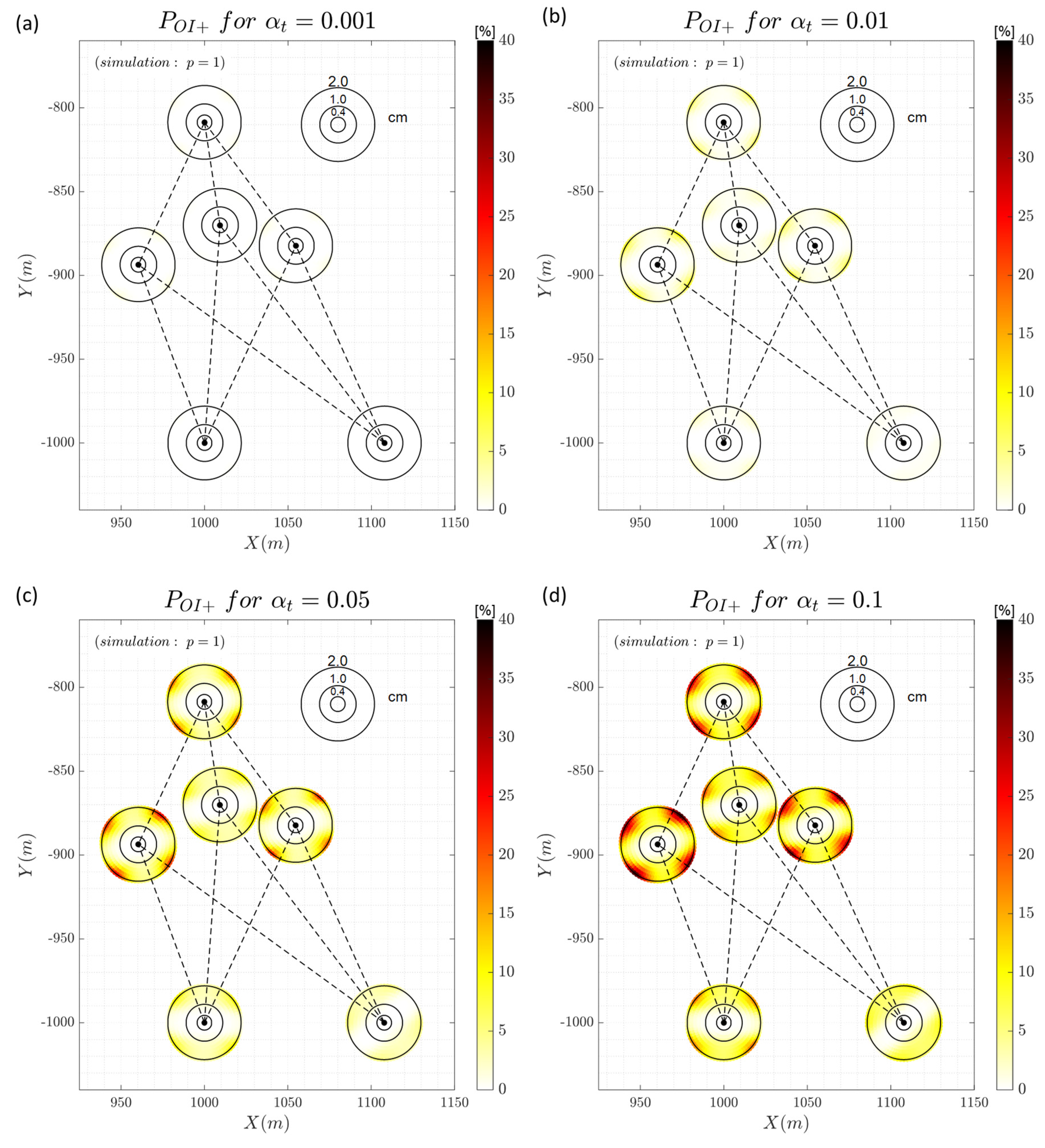
Figure 11.
Cumulative probability for the identification and detection success rates for , , and , and for the following cases: (a) for , (b) for , (c) for , (d) for , (e) for and (f) for .
Figure 11.
Cumulative probability for the identification and detection success rates for , , and , and for the following cases: (a) for , (b) for , (c) for , (d) for , (e) for and (f) for .
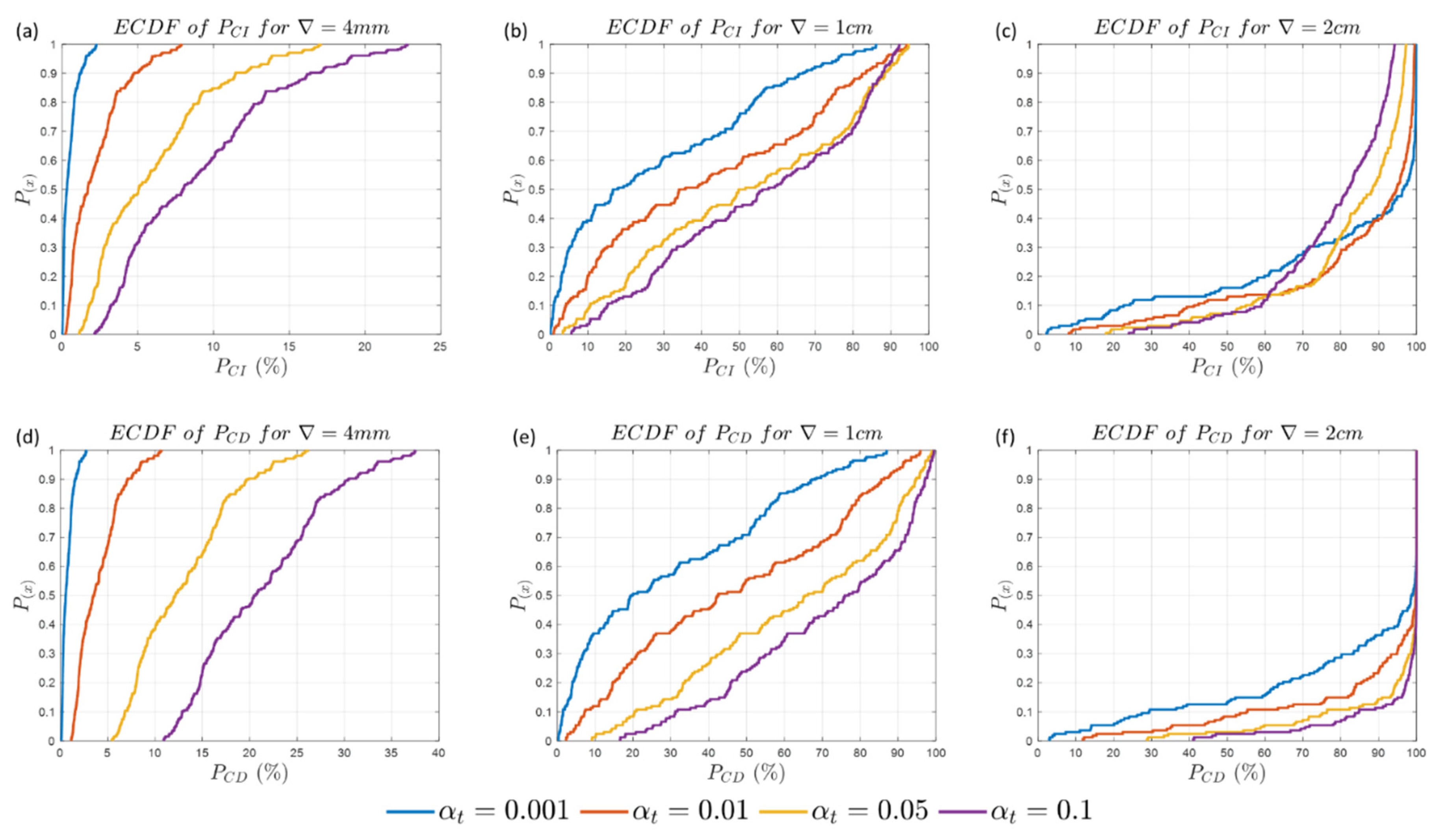
Figure 12.
Simulated displacement patterns for each group of two points ( and for first and second selected point).
Figure 12.
Simulated displacement patterns for each group of two points ( and for first and second selected point).
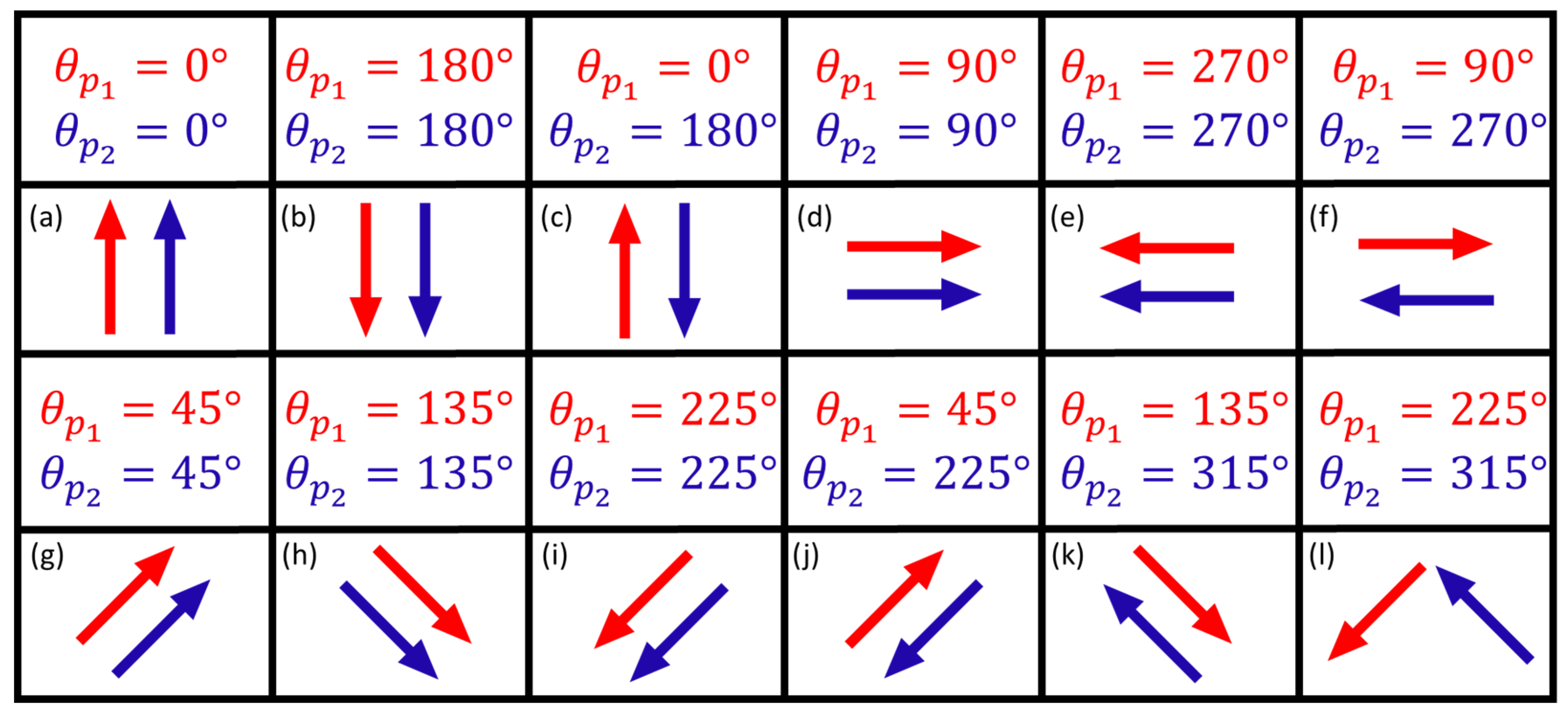
Figure 13.
Simulated displacement patterns for each group of three points (, and for first, second and third selected point).
Figure 13.
Simulated displacement patterns for each group of three points (, and for first, second and third selected point).
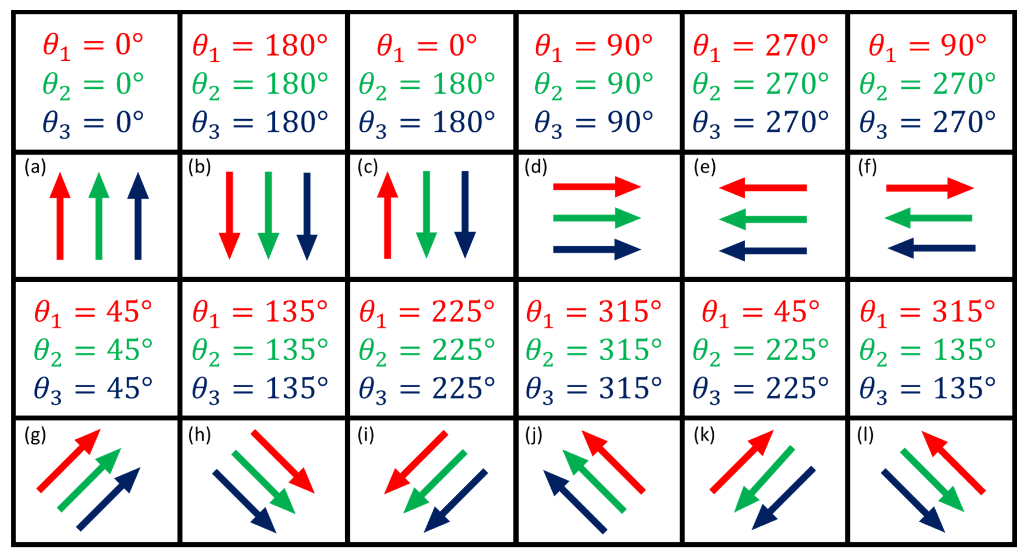
Figure 14.
Displacement patterns applied in the field: (a) displacement for each individual point at a time in the direction, denoted by ; (b) displacement for each individual point at a time in the direction, denoted by ; (c) displacement for each individual point at a time in the direction, denoted by ; (d) displacement for each individual point at a time in the direction, denoted by ; (e,f,g) displacement for two-point group simultaneous displacement, with the first point shifted in the direction and the second one in the direction; (h,i,j) displacement for three-point group simultaneous displacement, with the first point shifted in the direction, second point in the direction and the third one in the direction.
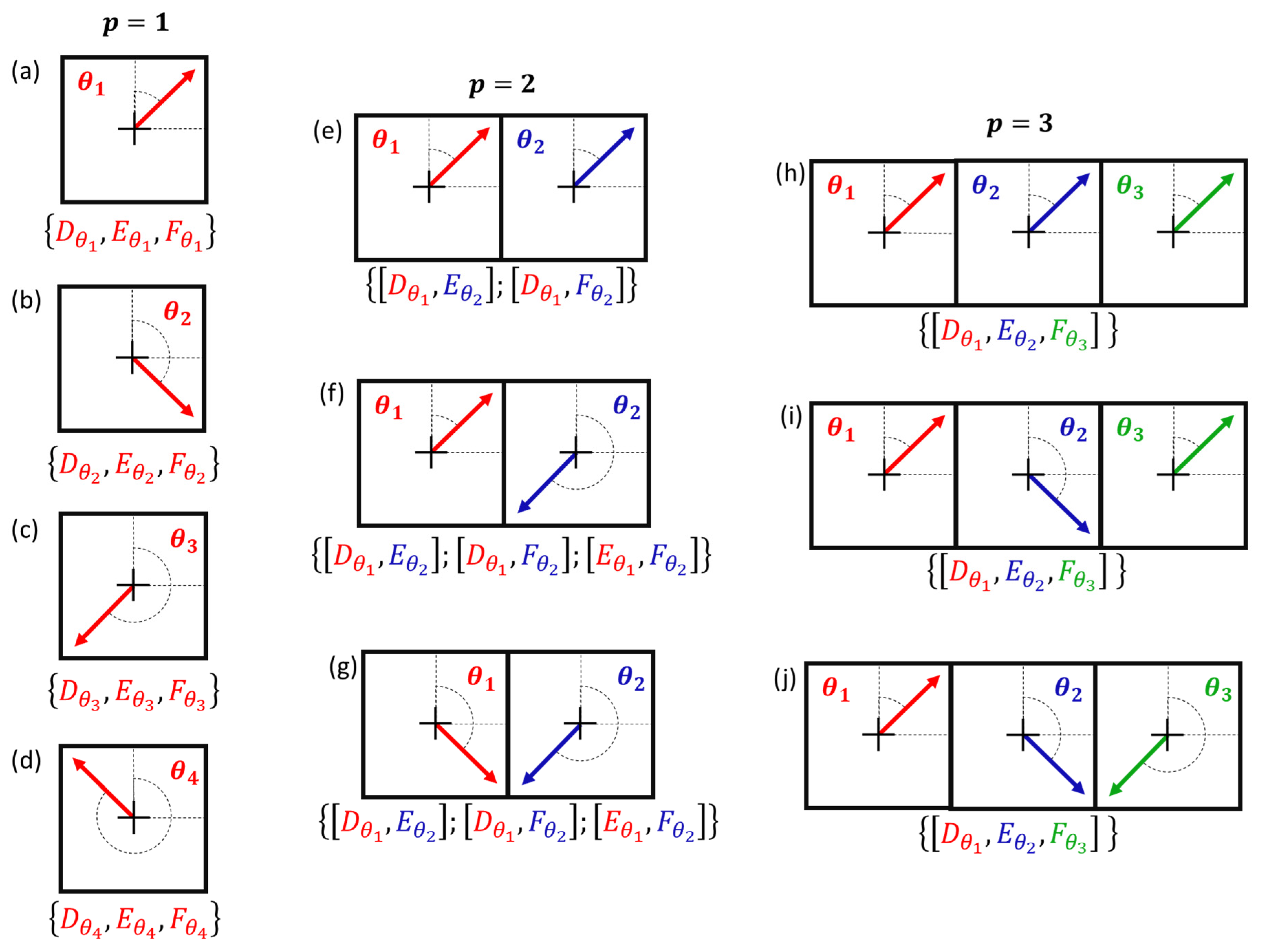

Table 1.
Coordinates of the network points for Epoch 1.
| Point | X [m] | Y [m] |
|---|---|---|
| A | 1000 | -1000 |
| B | 1107.83 | -1000 |
| C | 999.949 | -808.661 |
| D | 1054.73 | -882.298 |
| E | 1009.24 | -870.129 |
| F | 960.33 | -893.626 |
Table 2.
Distances of the segments for Epoch 1.
| Segment | True Distance [m] |
 |
129.8025 |
 |
130.1994 |
 |
113.5303 |
 |
129.1275 |
 |
163.0530 |
 |
181.8570 |
 |
91.7765 |
 |
62.1665 |
 |
93.7482 |
Table 3.
False positive rates for the critical values derived from Monte Carlo approach.
| 0.001 | 16.75 | ~0.001 | 0.00% |
| 0.01 | 12.27 | ~0.01 | 0.01% |
| 0.05 | 9.06 | ~0.05 | 0.03% |
| 0.1 | 7.62 | ~0.1 | 0.05% |
Table 4.
Maximum and minimum correct identification rate for two points mutually unstable .
| Displacement patterns | ||||||||||
| (a, b) | (c) | (d, e) | (f) | (g, i) | (h) | (j) | (k) | (l) | ||
| 0.1% | 74.63 | 99.94 | 53.47 | 90.16 | 50.64 | 69.63 | 91.2 | 99.95 | 85.87 | |
| 00.99 | 18.27 | 0.00 | 00.04 | 00.00 | 00.00 | 00.03 | 9.99 | 00.24 | ||
| 1% | 74.39 | 99.71 | 72.08 | 96.99 | 65.62 | 70.62 | 97.11 | 99.82 | 86.59 | |
| 03.46 | 20.25 | 00.00 | 00.61 | 00.00 | 00.00 | 00.28 | 19.30 | 01.26 | ||
| 5% | 72.58 | 98.69 | 78.66 | 97.83 | 69.99 | 70.55 | 97.14 | 99.14 | 83.75 | |
| 04.67 | 19.96 | 00.01 | 02.67 | 00.02 | 00.02 | 00.94 | 24.64 | 03.48 | ||
| 10% | 70.72 | 97.55 | 78.33 | 96.73 | 69.76 | 69.92 | 95.59 | 98.17 | 79.45 | |
| 04.78 | 19.38 | 00.02 | 04.45 | 00.05 | 00.05 | 01.30 | 25.76 | 05.29 | ||
Table 5.
Maximum and minimum correct detection rate for two points mutually unstable .
| Displacement patterns | ||||||||||
| (a, b) | (c) | (d, e) | (f) | (g, i) | (h) | (j) | (k) | (l) | ||
| 0.1% | 100.00 | 100.00 | 99.50 | 100.00 | 100.00 | 100.00 | 100.00 | 100.00 | 100.00 | |
| 80.63 | 95.50 | 30.87 | 45.04 | 21.73 | 21.82 | 66.71 | 68.14 | 82.80 | ||
| 1% | 100.00 | 100.00 | 99.96 | 100.00 | 100.00 | 100.00 | 100.00 | 100.00 | 100.00 | |
| 86.69 | 99.35 | 61.00 | 74.80 | 48.28 | 48.19 | 86.21 | 88.14 | 93.19 | ||
| 5% | 100.00 | 100.00 | 100.00 | 100.00 | 100.00 | 100.00 | 100.00 | 100.00 | 100.00 | |
| 93.10 | 99.95 | 81.59 | 91.52 | 72.10 | 71.97 | 95.64 | 96.68 | 98.16 | ||
| 10% | 100.00 | 100.00 | 100.00 | 100.00 | 100.00 | 100.00 | 100.00 | 100.00 | 100.00 | |
| 95.74 | 99.99 | 87.23 | 95.98 | 81.80 | 81.79 | 97.96 | 98.65 | 99.34 | ||
Table 6.
Maximum and minimum correct identification rate for three points mutually unstable .
| Displacement patterns | |||||||||
| (a, b) | (c) | (d, e) | (f) | (g, i) | (h, j) | (k) | (l) | ||
| 0.1% | 0.17 | 37.98 | 0.07 | 1.54 | 1.55 | 0.43 | 28.21 | 47.89 | |
| 0.00 | 0.00 | 0.00 | 0.00 | 0.00 | 0.00 | 0.00 | 0.00 | ||
| 1% | 0.69 | 38.16 | 0.64 | 8.22 | 5.23 | 0.56 | 40.69 | 47.94 | |
| 0.00 | 0.00 | 0.00 | 0.00 | 0.00 | 0.00 | 0.00 | 0.00 | ||
| 5% | 1.42 | 38.38 | 2.13 | 19.25 | 12.79 | 0.90 | 45.66 | 47.97 | |
| 0.00 | 0.00 | 0.00 | 0.00 | 0.00 | 0.00 | 0.00 | 0.01 | ||
| 10% | 1.76 | 37.86 | 3.17 | 25.17 | 18.20 | 1.21 | 46.51 | 48.07 | |
| 0.00 | 0.00 | 0.00 | 0.01 | 0.00 | 0.00 | 0.00 | 0.03 | ||
Table 7.
Maximum and minimum correct detection rate for three points mutually unstable .
| Displacement patterns | |||||||||
| (a, b) | (c) | (d, e) | (f) | (g, i) | (h, j) | (k) | (l) | ||
| 0.1% | 100.00 | 100.00 | 99.89 | 100.00 | 100.00 | 100.00 | 100.00 | 100.00 | |
| 85.79 | 89.16 | 32.39 | 76.51 | 37.27 | 82.02 | 29.50 | 69.40 | ||
| 1% | 100.00 | 100.00 | 99.99 | 100.00 | 100.00 | 100.00 | 100.00 | 100.00 | |
| 91.40 | 95.67 | 61.30 | 91.64 | 66.78 | 89.69 | 57.19 | 83.23 | ||
| 5% | 100.00 | 100.00 | 100.00 | 100.00 | 100.00 | 100.00 | 100.00 | 100.00 | |
| 93.98 | 98.38 | 79.75 | 97.47 | 86.30 | 94.78 | 78.75 | 91.10 | ||
| 10% | 100.00 | 100.00 | 100.00 | 100.00 | 100.00 | 100.00 | 100.00 | 100.00 | |
| 94.74 | 99.14 | 85.83 | 98.72 | 92.50 | 95.66 | 86.64 | 93.80 | ||
Table 8.
Frequency of occurrence for each SLRTUPI decision class for the case where all points are subject to be monitored.
Table 8.
Frequency of occurrence for each SLRTUPI decision class for the case where all points are subject to be monitored.
| Displace. patterns | Correct Detection | Correct Identification | Wrong Identification |
|---|---|---|---|
| (a) | 3 | 3 | 0 |
| (b) | 3 | 3 | 0 |
| (c) | 3 | 2 | 1 |
| (d) | 3 | 3 | 0 |
| (e) | 2 | 0 | 2 |
| (f) | 3 | 1 | 2 |
| (g) | 3 | 3 | 0 |
| (h) | 1 | 0 | 1 |
| (i) | 1 | 1 | 0 |
| (j) | 1 | 1 | 0 |
|
Total |
23 | 17 | 6 |
| Rate (%) | 100 | 73.91 | 26.09 |
Table 9.
Frequency of occurrence for each SLRTUPI decision class for the case where the points A, B and C are fixed as stable.
Table 9.
Frequency of occurrence for each SLRTUPI decision class for the case where the points A, B and C are fixed as stable.
| Displace. patterns | Correct Detection | Correct Identification | Wrong Identification |
|---|---|---|---|
| (a) | 3 | 3 | 0 |
| (b) | 3 | 3 | 0 |
| (c) | 3 | 3 | 0 |
| (d) | 3 | 3 | 0 |
| (e) | 2 | 2 | 0 |
| (f) | 3 | 2 | 1 |
| (g) | 3 | 3 | 0 |
| (h) | 1 | 1 | 0 |
| (i) | 1 | 1 | 0 |
| (j) | 1 | 1 | 0 |
| Total | 23 | 22 | 1 |
| Rate (%) | 100 | 95.65 | 4.35 |
Disclaimer/Publisher’s Note: The statements, opinions and data contained in all publications are solely those of the individual author(s) and contributor(s) and not of MDPI and/or the editor(s). MDPI and/or the editor(s) disclaim responsibility for any injury to people or property resulting from any ideas, methods, instructions or products referred to in the content. |
© 2023 by the authors. Licensee MDPI, Basel, Switzerland. This article is an open access article distributed under the terms and conditions of the Creative Commons Attribution (CC BY) license (http://creativecommons.org/licenses/by/4.0/).
Copyright: This open access article is published under a Creative Commons CC BY 4.0 license, which permit the free download, distribution, and reuse, provided that the author and preprint are cited in any reuse.


