Submitted:
19 December 2023
Posted:
20 December 2023
You are already at the latest version
Abstract
This work studies the discontinuities features of sedimentary flysch materials in a 100 km2 area belonging to the Basque Arc. Such materials are common in this Spanish Alpine region located in the north of the Iberian Peninsula. A total of 33 outcrops are investigated by an intensive geotechnical investigation including geomechanical stations, boreholes and mechanical laboratory tests. Two flysch units are characterized: the Upper Aguinaga Formation or siliciclastic flysch, and the Lower Itziar Formation or calcareous flysch. Differences between both flysch formation are found. Joints in the siliciclastic flysch formation present an undulated roughness, with a spacing narrower and a persistence lower than in the calcareous flysch formation, which exhibits higher friction angles, although roughness is essentially planar. In addition, the potential of using Artificial Intelligence (AI) techniques, particularly Artificial Neural Networks and Support Vector Machine, to estimate the Geological Strength Index (GSI) from the Rock Quality Design (RQD) and some discontinuities features (spacing, persistence, aperture and roughness) is investigated. AI techniques are found to be satisfactory, being the Support Vector Machine with a linear kernel the technique which achieves the best performance.
Keywords:
Flysch materials
; Geomechanical characterization
; Discontinuities
; Geological Strength Index
; AI tools
; Artificial Neural Network
; Support Vector Machine
1. Introduction
Unlike soils, the geomechanical behavior of rock masses is conditioned by discontinuities. In sedimentary rock masses, common discontinuities include bedding planes (stratification), faults and joints. Discontinuities may cause addressing the geomechanical behavior of rock masses to be difficult, so traditionally, geomechanically classifications like Bieniawski’s RMR [1] or Barton’s Q index [2] are used. When only discontinuities are to be considered, the Geological Strength Index, GSI [3,4], provides a good insight of the state of the rock mass. One of the main uses of the GSI is as an input of the well-known Generalized Hoek-Brown failure criterion [5].
Among the different geological materials, sedimentary flysch formations are a common source of slope instabilities and other geotechnical problems, which many times appear during the construction phase of a project (like roads and railways) or afterwards, during its exploitation phase. This issue increases the environmental impact of such projects, and it also contributes to increase their carbon footprint as more work actions are needed to be conducted. A good understanding of the behavior of those challenging materials is therefore essential to ensure a sustainable approach.
In Spain, flysch formations can be found in the Basque Arc, an area geologically belonging to the Basque-Cantabrian Basin, an inverted Mesozoic extensional basin, connecting the Pyrenees in the East and the Cantabrian Mountains in the West. In previous research [6], the authors studied such flysch materials, in particular the ones found in an area of approximately 100 km2 around the town of Astigarraga (Basque Country, Spain). That work aimed at characterizing the rock mass following the classification proposed by Morales et al. [7]. These authors use the GSI modified for flysch formations [4] and the uniaxial compressive strength of the intact rock to define the rock mass properties (in terms of Hoek-Brown parameters).
The present work studies the flysch materials on such area, but it is focused on the discontinuity’s features. The work makes use of a broad geological-geotechnical investigation involving 40 boreholes, laboratory tests on 124 undisturbed rock samples and geomechanical stations on 33 locations. Additionally, two Artificial Intelligence (AI) techniques were used to estimate the GSI for flysch materials from the Rock Quality Design, RQD [8], and four discontinuity features (spacing, persistence, aperture and roughness). The GSI is a geomechanical index envisage to be easily obtained in field using a chart, based on the description of the rock mass geological structure and the discontinuities surface condition. This procedure requires some practitioner experience though. Some authors [9,10,11] proposed a more quantitative approach to obtain the GSI, but such expressions are designed for hard rocks and not very heterogeneous formations like flysch. Therefore, the GSI definition for flysch materials still relays on practitioner experience. AI techniques can provide an alternative way of yielding quantitative expression to define this index. It should be note that AI integration is becoming a common practice in a sustainable approach of geotechnical problems, since it helps in the analysis of complex geological data, reduces the need for extensive field surveys and optimizes resource usage. In this work, Artificial Neural Networks (ANNs) and Support Vector Machine (SVM) AI techniques were selected. ANN is of common use in civil and geotechnical engineering [12,13,14,15,16,17] while SVM has also been used in geological engineering for solving multiclass problems [12,18,19].
2. Geographical and geological setting
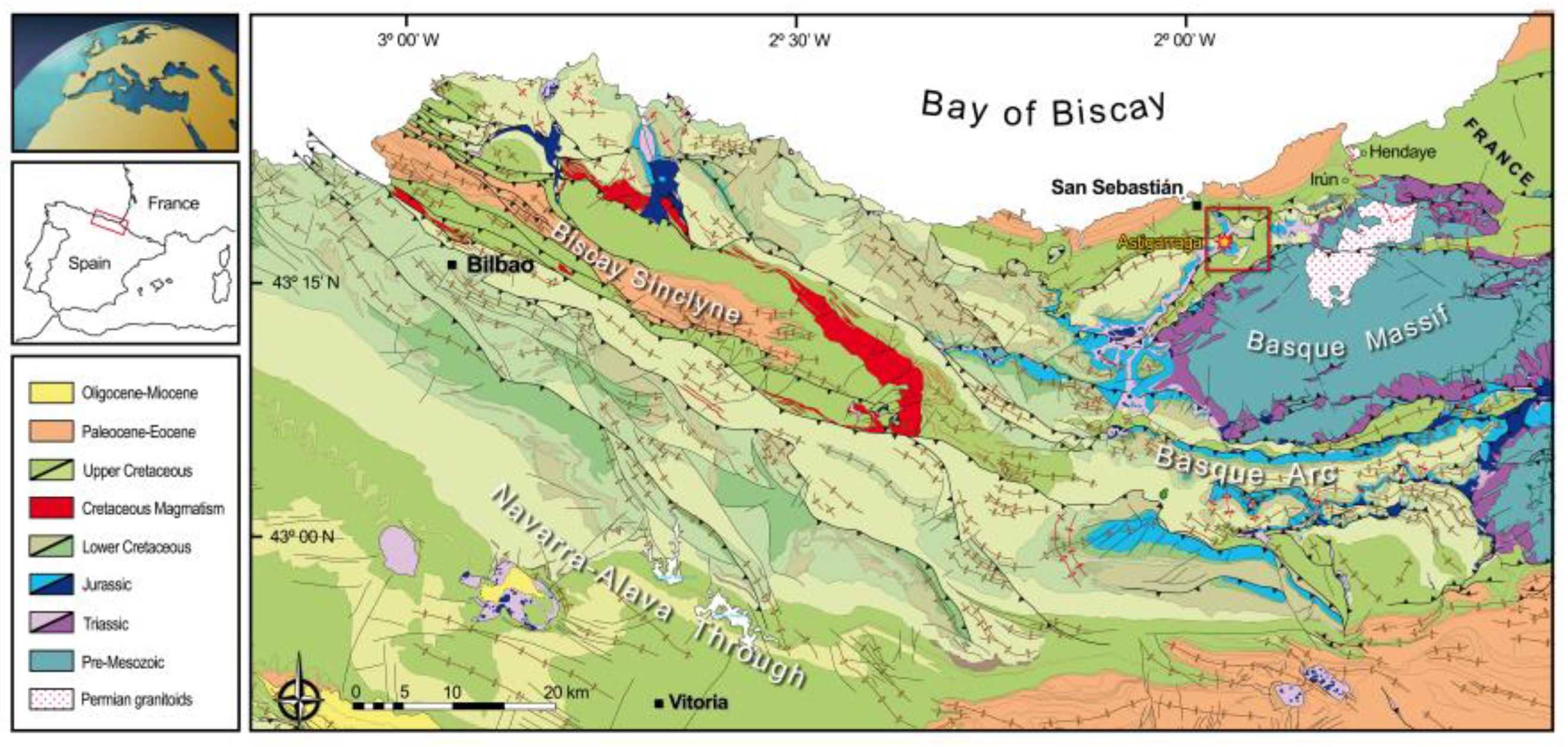
The study area lies in the Basque-Cantabrian Basin, located in the northern Iberian margin (Figure 1). The basin consists of a Mesozoic salt-bearing narrow rift basin [20,21] inverted during the Alpine orogeny [22,23]. The Mesozoic extension can be subdivided into two rift periods. The first phase took place from Permian to Triassic times [24,25], followed by a tectonic quiescence phase from Early to Middle Jurassic times [26]. The opening of the North Atlantic and the Bay of Biscay-Pyrenean rift system triggered the main and second rifting phase during the Late Jurassic and Early Cretaceous times (e.g. [27,28,29]). Overall, the basin is filled by several kilometers of a succession composed of marine carbonate and coastal siliciclastic deposits [28]. From Late Cretaceous to Miocene times, the rift basin was inverted due to the convergence between Iberia and Eurasia, resulting in the development of the E-W oriented orogenic Pyrenean-Cantabrian belt along the northern Iberian plate margin [30,31,32]. The synorogenic sedimentary record is mostly characterized by clastic material deposited and preserved in the Villarcayo and Bureba synclinal sub-basins, and especially in the Duero and Ebro foreland basins. The junction between them presents a drainage system controlled by the Miocene to present-day tectonic regime [33].
West of the Paleozoic Cinco Villas Massif lies the Basque Arc, a south and north-verging thrust belt (Figure 1), characterized by its arched shape and considered as the most intensively deformed area of the Basque-Cantabrian Basin [34]. This tectonic arc is affected by NW- and NE-directed thrust faults, sub-vertical strike-slip faults and NW-SE oriented major folds, which are represented by the Bilbao anticlinorium, the Biscay synclinorium and North-Biscay anticlinorium from south to north [35].
Figure 1.
Simplified geologic map of the eastern portion of the Basque-Cantabrian Basin showing the location of the study area (star). Inset indicates the location of the detailed map depicted in Figure 2. Modified from [6,35].
The study area is based on a railway track running through an area located between the Cinco Villas Massif and the eastern termination of the North-Biscay anticlinorium. The track consists of an 8-km-long projected stretch of the high-speed Vitoria-Bilbao-San Sebastian railway line that will connect, from north to south, the locations of Rentería and Hernani through the Astigarraga village (Figure 2). The construction of the railway will encounter a wide range of different lithologies which recorded the Mesozoic paleogeographic evolution of the Basque-Cantabrian Basin in the region.
The Mesozoic sedimentary record in the area starts with the Late Triassic extension phase, which is represented in by a thick package of evaporites and shales with dolerite intrusions, the so-called Keuper Formation [36,37]. This salt unit is responsible for the diapirism and constitute the main detachment level for the thin-skinned deformation in the Basque-Cantabrian Basin and the Pyrenees [38,39,40,41,42]. A thick package of limestones, dolostones and marlstones was deposited on top of the evaporite unit as result of the regional sag-type subsidence after the first rifting phase [43,44,45]. The Lower Jurassic dolostones act as a reservoir for the CO2 geological storage pilot plant of Hontomín in the southernmost portion of the Basque-Cantabrian Basin (e.g. [46]). The second rift phase starts with the deposition of Urgonian reef limestones with intercalations of sandstones, claystones and marlstones of Aptian to Early Albian in age. The syn-rift infilling resumed with the Oiartzum Formation (late Albian to early Cenomanian), represented by fluvial to transitional conglomerates, sandy calcarenites and sandstones. The following succession consists of a turbiditic unit (calcareous and siliciclastic flysch facies) deposited in a deep open marine environment from Campanian to Early Paleogene times. The Meso-Cenozoic basin is overlain by Quaternary fluvial and colluvial deposits (Figure 2).
Figure 2.
Detailed geologic map and schematic stratigraphic section of the studied area showing sample locations (33) on the “Calcareous Flysch” (blue stars) and the “Siliciclastic Flysch” (red stars). Modified from [6,47].
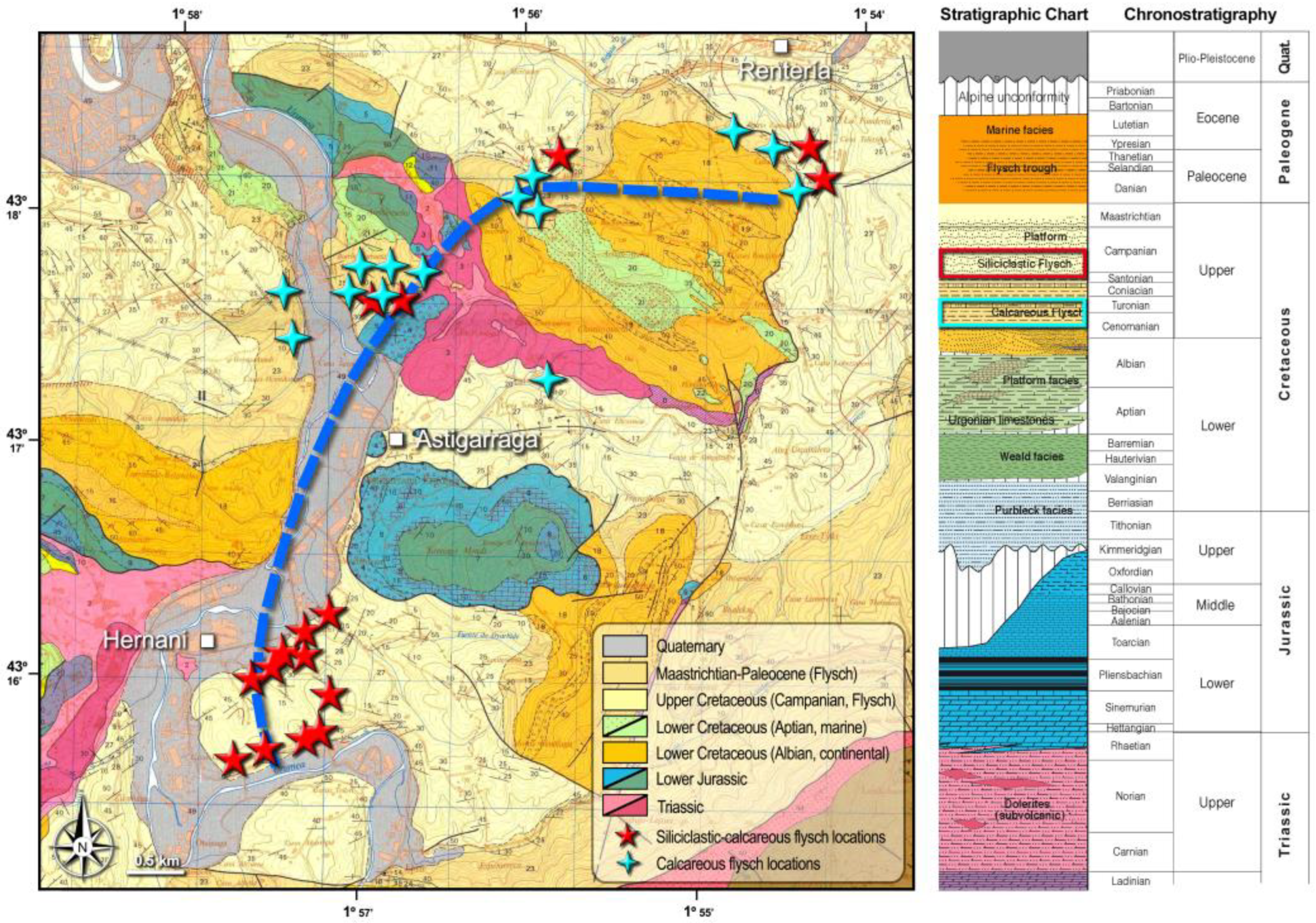
The present work comprises data obtained from the Upper Cretaceous turbiditic sequences, also known as the “Upper Cretaceous flysch” [47]. The flysch formation is represented by a relatively thick package of more than 700 m of interbedded marlstones and marly limestones, changing to quartz-rich clastic turbidites towards the top of the succession. Thus, two main units can be differentiated in terms of their lithology and timing of deposition: 1) the Lower Itziar Formation or “calcareous flysch” (Cenomanian-Turonian); and 2) the Upper Aguinaga Formation or “siliciclastic flysch” (Santonian-Campanian) [48]. These formations were deposited at the initial stages of the convergence between Eurasia and Iberia in an intraplate trough, inherited from smaller rift basins developed in the Basque-Cantabrian Basin [49,50,51]. The water depth is estimated between 800 to 1500 m in which the sediments were deposited in hemipelagic settings during an increased subsidence stage. A subsequent relative tectonic quiescence highly decreased the subsidence from Maastrichtian to Paleocene times [51].
3. Materials and Methods
3.1. Field tests
A comprehensive geological-geotechnical investigation was performed, including 24 petrographic analyses, 33 geomechanical stations and 40 boreholes. A total of 33 locations (outcrops) were studied, 18 in the upper flysch unit and 15 in the lower flysch unit. Boreholes were drilled with an 89 mm core drill, ranging from depths of 16 to 114 meters.
Geomechanical stations provided insights into the composition of intact rock and any structural irregularities, detailing their types (such as joints and faults), orientations and key properties like spacing, persistence and aperture. To assess the rock's overall fracturing state, discontinuities were analyzed through stereographic projection. This projection method involves categorizing these irregularities based on shared characteristics.
3.2. Laboratory tests
A total of 124 undisturbed rock samples were collected for various laboratory tests, including uniaxial compressive strength, point load, Brazilian and triaxial tests [6]. Direct shear tests were conducted to determine the angle of friction for rock joints. Identification tests, such as unit weight measurement, were also performed. These tests followed ISRM [52,53] and ASTM standards [54,55,56,57,58]. The RQD value was either directly obtained from borehole data through drilling or calculated using Palmström’s [59] correlation method, based on the volumetric joint count value (Jv) and obtained from geomechanical stations.
3.3. Artficial Neural Networks
Current ANN algorithms are based on the backpropagation neuron [60]. In this work, the Matlab commercial software v. R2023, especially the Neural Network Toolbox, was used to build a series of feedforward multilayer perceptron networks. In essence, such kind of ANNs consists of a series of interconnected layers (Figure 3), with each layer containing a series of neurons connected to all neurons located in previous and following layers (but not in the same layer). A neuron (1) receives a value from each neuron in the previous layer, (2) linearly combines such values according to a series of weights (which correspond to the interconnection with the other neurons) and (3) delivers the output by applying a “transfer function” to the result of the linear combination. The first layer of neurons is the “input layer” and contains the input values of the system. Therefore, its number of neurons is equal to the number of inputs and no lineal combination nor transfer function is applied. The last layer, or “output layer”, contains a number of neurons equal to the number of outputs of the system. Layers between the input and output ones are called “hidden layers” and the neuron at them “hidden neurons”. The number of hidden layers and neurons is unknown and depends on the problem under study (e.g. [16,17]).
To set the weights of each linear combination on each neuron, ANNs are trained by cases where inputs and their corresponding outputs are known. The Lavenberg–Marquardt algorithm with back-propagation was used in this work to train the ANNs. Basically, starting from random weights, the ANN is run and the error between the computed outputs (given by the ANN) and the target outputs (known value) is propagated backwards, modifying the weights. The process is continued until an error predictor is reduced to a certain value (or until a maximum number of iterations or epochs is reached). As a predictor, the Mean Squared Error (MSE) is normally used:
where Ti is the target output; and Oi is the computed output.
Performance of an ANN developed is assessed at training as well as by testing it against other cases not used for training where inputs and their corresponding outputs are known. Coefficient of determination R2, MSE and other common statistical parameters are used. If a satisfactory performance is achieved, the resulting ANN can be used as a pretrained regressor to make predictions.
In this work, 70% of the available data was randomly selected for training. The remaining 30% was used for testing. Number of epochs was set to 3000. One hidden layer was defined, selecting a sigmoid function as the transfer function for hidden neuron. In the output layer (with only one output neuron, the GSI), a linear function was set as transfer function. Taking that into account, the ANNs developed can be mathematically expressed as:
where inputi is a vector with the value of the corresponding input variables; α and β are two numbers corresponding to the weight and the bias of the output neuron; ωi is the vector with the weights of the hidden neurons and ω0 is the bias of such hidden layer. Index j corresponds to the number of hidden neurons, normally found between the number of inputs and outputs and established by a trial and error process [16,17].
Equation (2) is a pretrained regressor that allows obtaining the output value of the ANN by a mathematic expression (e.g. [13]). However, to ensure the stability of the training process and obtain a higher degree of accuracy, input and output data should be normalized before developing any ANN, and such normalization must be considered in Equation (2). In this work, normalization was done by dividing each variable by the maximum value attained for the variable considered. For instance, for a given input:
where max(input) refers to the maximum value that such input takes for the whole data considered.
A total of 20 network architectures 27-X-1 were set (being 27 the number of input neurons, see 4.3, X the number of hidden neurons and 1 the output neuron, the GSI), ranging the number of hidden neurons X from 5 to 25. For each architecture, 100 models were considered (this means running a total of 2000 models) to find the optimum ANN with the best performance for each architecture both at training and testing.
3.4. Support Vector Machine
The SVM technique appeared in the early sixties [61] and consists of using algebraic methods to find linear decision boundaries (“hyperplanes”) that separate variables. If data are nonlinear, a kernel function (linear, polynomial and sigmoidal) [62,63] may be used to transform such data into higher dimensions, where finding the hyperplanes is possible. In this work, the Matlab commercial software v. R2023 was used to apply the SVM technique, particularly the Deep Learning Toolbox and the function “fitcecoc”.
Like ANN, training of SVM is done by cases where inputs and their corresponding outputs are known. However, training of a SVM algorithm is similar to solving a quadratic programming problem. The objective is finding the best hyperplane with the largest “margin”, i.e. a hyperplane with the maximum width of the slab parallel to the hyperplane (margin) with no interior data points. For instance, given a linear hyperplane f(x) defined by a parameter β, the aim is minimizing the norm of β so the margin is maximum. This is done by maximizing a series of Lagrange multipliers αj that optimized the expression:
where yj is the output data and xj are the data vectors corresponding to the inputs. The term Σαjyjxj corresponds to the hyperplane (parameter β). Data points xj corresponding to nonzero αj values are called support vectors.
Performance of SVM developed is, as in the case of ANN, assessed at training as well as at testing against other cases not used for training where inputs and their corresponding outputs are known (using R2, MSE and other statistical parameters). If an acceptable performance is achieved, the resulting SVM can be used as a pretrained regressor to make predictions. Unlike ANN, SVM does not need the input and output data to be normalized, but, due to its algebraic nature, the pretrained regressor cannot be easily written as a simple mathematical expression.
As in the case of the ANN developed, in this work 70% of the available data was randomly selected for training, using the remaining 30% of data for testing. Two kernel functions were considered: linear and gaussian (radial basis function). For each kernel function, 1000 models were considered to find the optimum SVM model with the best performance.
4. Results
4.1. Field tests
Geomechanical assessments of flysch materials indicated the presence of at least three sets of discontinuities, occasionally four. Notably, no faults were found in either flysch unit. These findings align with the ISRM (1981) classification, which categorizes the level of fracturing in the studied rock masses as class VI ("three sets of discontinuities") and class VII ("three sets of discontinuities plus an occasional one"). Furthermore, the block shape observed in the slope inventory revealed that the rock masses analyzed primarily consisted of tabular-prismatic blocks, often vertically flattened and occasionally exhibiting a planar shape. This block morphology is characteristic of flysch deposits.
The discontinuities structural parameters were recorded in each outcrop from the two studied flysch units (Figure 4). Most of the studied outcrops related to the siliciclastic flysch formation are represented by 20 to 200 mm in terms of spacing. For the carbonated flysch formation, the spacing increased, ranging from 20 to 600 mm.
In terms of persistence strike/dip parameter, the siliciclastic flysch is characterized by very low (< 1 m) to low (1 – 3 m) values, while the carbonated flysch is mainly represented by low persistence values. The rock fracture aperture is also differentiated between the two formations. The siliciclastic flysch shows two types of apertures, very tight (< 0.1 mm) to tight (0.1 – 0.25 mm) and opened to moderately wide (2.5 –10 mm), whereas the highest values of the carbonated flysch outcrops are concentrated in the very tight to tight aperture. The undulated roughness, both rough and smooth, is representative of the siliciclastic flysch, followed by the irregular roughness (rough). The carbonated flysch presents the highest values related with planar roughness (rough and smooth), followed by undulated (smooth). The seepage also shows notable differences between both units, where most of the outcrops of the siliciclastic flysch unit are dry, while those in the carbonated flysch are mostly wet.
4.2. Laboratory tests
The laboratory analyses and mechanical testing results, encompassing parameters such as unit weight, uniaxial compressive strength, tensile strength, point load index, confined compression, and shear strength of joints, are summarized in Table 2. Siliciclastic flysch materials displayed an average dry unit weight of 26.4 kN/m³, with an average uniaxial compressive strength of 24.83 MPa and a tensile strength averaging 8.43 MPa. The triaxial test conducted under confined compression conditions revealed average values of 10 MPa for cohesion and a 40° friction angle for the intact rock, while the average residual friction angle of joints within this formation was determined to be 23°.
Calcareous flysch materials exhibited an average dry unit weight of 26.4 kN/m³, with an average uniaxial compressive strength of 22.89 MPa and a tensile strength averaging 6.49 MPa. The triaxial test under confined compression yielded average values of 8.6 MPa for cohesion and a 49° friction angle for the intact rock, along with an average residual friction angle of 30° for the joints within this formation.
4.3. Data for ANN and SVM models developed
Field data obtained in the characterization of the discontinuities studied were used to train and test the ANN and SVM models developed to estimate the GSI. The input parameters considered were RQD, spacing, persistence, aperture and roughness. The RQD value was introduced directly (previously normalized for the ANN models, dividing it by 100, maximum theoretical value for RQD). The discontinuities features were considered in terms of the ranges used for their characterization. This means 7 variables for spacing (< 20 cm extremely narrow, 20 – 60 cm very narrow, 60 – 200 cm narrow, 200 – 600 cm moderately narrow, 600 – 2000 cm wide, 2000 – 6000 cm very wide and > 6000 cm extremely wide), 5 for persistence (< 1 m very low, 1 – 3 m low, 3 – 10 m medium, 10 – 20 m high and > 20 m very high), 9 for aperture (< 0.1 mm very tight, 0.1 – 0.25 mm tight, 0.25 – 0.5 mm partially opened, 0.5 – 2.5 mm opened, 2.5 – 10 mm partially wide, > 10 mm very wide, 10 – 100, 100 – 1000 mm extremely wide and > 1000 mm cavernous) and 9 for roughness (irregular-rough, irregular-smooth, irregular-slickensided, waved-rough, waved-smooth, waved-slickensided, planar-rough, planar-smooth and planar-slickensided). Each variable was introduced in terms of the percentage that the variable represents against the rest of possible ranges for the same feature; values were normalized to the maximum for ANN models.
All in all, the total number of variables to consider as inputs in the AI models would be 31. However, since some discontinuities feature ranges were always null (spacing > 6000 cm, aperture 100 – 1000 mm and > 1000 mm, and roughness planar-slickensided), these variables were removed from the data for the AI techniques developed to avoid including noise. That resulted in considering 27 variables (RQD, 6 for spacing, 5 for persistence, 7 for aperture and 8 for roughness) as inputs for the ANN and SVM models developed.
4.4. ANN and SVM results
Table 3 shows the best performance reached by each model developed using the AI techniques ANN and SVM. As training performance achieved very satisfactory results in all cases (with low MSE values and R2 very close to 1), for the sake of brevity, these values are not included here. Only testing performance is shown. To complement the analysis, maximum, minimum and average value of the ratio between the GSI computed using the pretrained regressor obtained with each AI model and the GSI measured on field is shown. The term ANN_27-X-1, with X equal to the number of hidden neurons, is used for referring to the ANN developed, while SVM_linear and SVM_radial refer to SVM models developed considering a linear or radial (gaussian) kernel, respectively.
A general inspection of the statistical predictors reveals that the ANN technique struggles to find a satisfactory performance. In terms of R2, the best model is ANN_27-14-1 with R2 = 0.91, being the MSE 115 and the value of predictors considered for the ratio between the GSI computed and the GSI measured very acceptable: minimum of such ratio is close to 1.0, average has an error about 20 % and maximum of 65 %. The next best model in terms of R2 is ANN_27-12-1 with R2 = 0.88 and MSE = 147, but the value of predictors for the ratio between the GSI computed and the GSI measured are very poor (average and minimum are far from 1.0, especially the second one).
If the MSE predictor is considered, the best ANN model corresponds to ANN_27-17-1, with R2 = 0.75 and MSE = 82, and while maximum and average values for the ratio between the GSI computed and the GSI measured are good, the minimum is poor. The next best model in terms of MSE is ANN_27-9-1 with R2 = 0.74 and MSE = 84, and with acceptable values of the ratio between the GSI computed and the GSI measured (average 1.13, maximum 1.53, minimum 0.71). Taking into account such ratio as the main predictor, the best models can be considered ANN_27-9-1, second best model in terms of MSE, and ANN_27-14-1, best model in terms of R2, as well as ANN_27-7-1, which achieves R2 = 0.70 and MSE = 91. Thus, considering all statistical predictors, the model ANN_27-14-1 (14 hidden neurons) may be selected as the ANN model that reaches the best performance: low MSE, R2 close to 1.0 and ratio between the GSI computed and the GSI measured close to 1.0.
Regarding the SVM models, the best model is SVM_linear, which achieves R2 = 0.88 and MSE = 51 (a very low value), as well as satisfactory values of the ratio between the GSI computed and the GSI measured (average 0.94, maximum 1.12, minimum 0.51). SVM_radial does not attain such good performance, especially in terms of MSE (182) and R2 (0.70), but values for the ratio between the GSI computed and the GSI measured are good and better than some ANN models.
To compare the performance of both AI tools used, Figure 5 shows the relationship between the GSI values experimentally obtained (all data, both used for testing and training) and the GSI values obtained using the best AI models, i.e. ANN_27-14-1 and SVM_linear. As observed, for the case under study, SVM technique appears to be more appropriate to estimate the GSI. Estimated values using SVM are closer to a perfect match (R2 = 1) and all values except one provide a GSI value with an error of less than 10 points (i.e. they are inside the GSI ± 10 buffer showed), which is a reasonable error for the GSI index (note that the definition of GSI for flysch materials is mainly qualitative). Conversely, several values estimated using ANN are not close to the R2 = 1 line and some of them give errors of more than 10 points from the experimental GSI value (they are outside the GSI ± 10 buffer).
5. Discussion and Conclusions
Flysch materials found in the area under study belonging to the Basque Arc (North of Iberian Peninsula) are geologically classify in two units [48]: the Lower Itziar Formation (calcareous flysch) and the Upper Aguinaga Formation (siliciclastic flysch). This distinction is also evidenced in the geomechanical characterization of the discontinuities of such materials. Differences observed in the structural parameters (Figure 4) highlight the unique characteristics of the two flysch units.
The variations in discontinuity spacing suggest differing rheological and diagenetic histories, with the siliciclastic flysch likely experiencing more frequent but narrower discontinuities compared to the carbonated flysch.
The persistence strike/dip values provide additional clues about the role of rock composition on the deformational processes these formations underwent. The low to very low persistence values in the siliciclastic flysch suggest a more localized failure related to a more heterogenous lithology, whereas the predominantly low persistence values in the carbonated flysch point towards a more homogeneous rock composition, where deformation is more consistently distributed.
The distinct rock fracture apertures further emphasize the heterogeneity between the formations. The siliciclastic flysch’s range of aperture types indicates varied mechanical properties, potentially linked to differences in lithology or stress regimes during formation. Meanwhile, the prevalence of very tight to tight apertures in the carbonated flysch suggests a more compact and less permeable rock matrix.
Surface roughness characteristics provide insight into the erosional and depositional processes that shaped these flysch formations. The prevalence of undulated roughness in the siliciclastic flysch suggests a history of fluctuating energy conditions, possibly related to changes in sediment transport dynamics. In contrast, the dominance of planar roughness in the carbonated flysch implies more uniform and stable depositional environments.
The contrasting seepage patterns not only reflect the current hydrological conditions but also hint at potential differences in the porosity and permeability of the two formations. The dry nature of most siliciclastic flysch outcrops suggests limited water infiltration, whereas the wet conditions in the carbonated flysch imply higher permeability and a greater potential for fluid flow through the rock, more likely to produce rock instabilities and slope movement.
Differences between siliciclastic flysch and calcareous flysch formations also exist when considering geomechanical parameters. Although both formations show similar average dry unit weights, uniaxial compression strength and tensile strength average values of the intact rock are slightly higher for the siliciclastic flysch formation. Nevertheless, the calcareous flysch formation exhibits higher friction angles for discontinuities (about 20% higher) and greater mechanical values (about 25% higher) for the intact rock under confined compression tests compared to siliciclastic flysch formation.
GSI estimation by SVM and ANN AI tools proves the ability of those techniques to define this geomechanical index in flysch materials. The analysis of the statistical predictors considered for the testing data (MSE, R2 and ratio of the GSI obtained by the AI model and the GSI measured on field) show satisfactory results. Comparing the two techniques used, SVM appears to be more appropriate to estimate the GSI, in particular the SVM with a linear kernel. This achieves a high value of R2 (0.88), very low value of MSE and an average ratio of the GSI estimated and the GSI measured close to 1.0. In addition, except 1 value, all GSI estimations show a deviation of less than 10 points from the GSI measured on field. The result obtained is relevant since a linear kernel does not usually reach a high performance when classifying not linear relationships [12]. This means either the relationship for flysch formations between the GSI and the variables considered (RQD and discontinuities features) is close to be linear or the SVM technique with a linear kernel is also capable of working satisfactorily with some non-linear relationships. More research is needed about this aspect. Finally, it should be note that AI integration is becoming a common practice in a sustainable approach of geotechnical problems, since it helps in the analysis of complex geological data, reduces the need for extensive field surveys and optimizes resource usage.
Author Contributions
Conceptualization, J.G.-R. and F.J.T.; methodology, J.G.-R. and A.R.; software, J.G.-R.; validation, J.G.-R., F.J.T. and M.J.R.-P.; formal analysis, F.J.T. and M.J.R.-P; investigation, J.G.-R. and A.R.; resources, J.G.-R. and F.J.T.; data curation, J.G.-R. and A.R.; writing—original draft preparation, J.G.-R. and A.R.; writing—review and editing, J.G.-R., F.J.T. and M.J.R.-P.; visualization, J.G.-R. and F.J.T; supervision, J.G.-R. and F.J.T.; project administration, F.J.T. All authors have read and agreed to the published version of the manuscript.
Funding
Financial support was provided by the Department of Geological and Geotechnical Engineering of the Universitat Politècnica de València and the research group “Planetary Geodynamics, Active Tectonics and Related Hazards” UCM-910368 of the Complutense University of Madrid.
Institutional Review Board Statement
Not applicable.
Informed Consent Statement
Not applicable.
Data Availability Statement
The data that support the findings of this study are available upon request from the corresponding authors.
Acknowledgments
The authors thank the Spanish companies PROYEX, S.A. and IBERGEOTECNIA, S.R.L. as well as the geologist M. Estefanía Bona, for providing the geotechnical data.
Conflicts of Interest
The authors declare no conflict of interest.
References
- Bieniawski, Z.T. Engineering rock mass classifications. John Wiley and Sons, Inc: New York, USA, 1989.
- Barton, N.; Lien, R.; Lunde, J. Engineering classification of rock masses for the design of tunnel support. Rock Mech. 1974, 6, 189–236. [Google Scholar] [CrossRef]
- Hoek, E. Rock engineering. Course Notes by Evert Hoek. Balkema: Rotterdam, The Netherlands, 2000.
- Marinos, P.; Hoek, E. Estimating the geotechnical properties of heterogeneous rock masses such as flysch. Bull. Eng. Geol. Env. 2001, 60, 82–92. [Google Scholar] [CrossRef]
- Hoek, E.; Carranza-Torres, C.; Corkum, B. Hoek-Brown failure criterion – 2002 Edition. Proc. NARMS-TAC Conference 2002, 1, 267-273.
- Garzón-Roca, J.; Torrijo, F.J.; Company, J.; Cobos, G. Geomechanical characterization and analysis of the Upper Cretaceous flysch materials found in the Basque Arc Alpine region. Bull. Eng. Geol. Environ. 2021, 80, 7831–7846. [Google Scholar] [CrossRef]
- Morales, T.; Uribe-Etxebarria, G.; Uriarte, J.A.; Fernández de Valderrama, I. Geomechanical characterisation of rock masses in Alpine regions: the Basque Arc (Basque-Cantabrian basin, Northern Spain). Eng. Geol. 2004, 71, 343–362. [Google Scholar] [CrossRef]
- Deere, D.U. Technical Description of Rock Cores for Engineering Purpose. Rock Mech. Eng. Geol. 1963, 1, 16–22. [Google Scholar]
- Sonmez, H.; Ulusay, R. Modification to the Geological Strength Index (GSI) and Their Applicability to Stability of Slopes. Int. J. Rock Mech. Min. Sci. 1999, 36, 743–760. [Google Scholar] [CrossRef]
- Cai, M.; Kaiser, P.K.; Uno, H.; Tasaka, Y.; Minami, M. Estimation of rock mass deformation modulus and strength of jointed hard rock masses using the GSI system. Int. J. Rock Mech. Min. Sci. 2004, 41, 3–19. [Google Scholar] [CrossRef]
- Hoek, E.; Carter, T.G.; Diederichs, M.S. Quantification of the Geological Strength Index Chart. In Proceedings of the 47th U.S. Rock Mechanics/Geomechanics Symposium, San Francisco, California, June 2013. [Google Scholar]
- Román-Herrera, J.C.; Rodríguez-Peces, M.J.; Garzón-Roca, J. Comparison between Machine Learning and Physical Models Applied to the Evaluation of Co-Seismic Landslide Hazard. Appl. Sci. 2023, 13, 8285. [Google Scholar] [CrossRef]
- Garzón-Roca, J.; Torrijo, F.J.; Alonso-Pandavenes, O.; Alija, S. Cerchar Abrasivity Index Estimation of Andesitic Rocks in Ecuador from Petrographical Properties Using Artificial Neural Networks. Int. J. Geomech. 2020, 20(5), 04020036. [Google Scholar] [CrossRef]
- Fattahi, H.; Bazdar, H. Applying improved artificial neural network models to evaluate drilling rate index. Tunnelling Underground Space Technol. 2017, 70, 114–124. [Google Scholar] [CrossRef]
- Nejad, F.P.; Jaksa, M.B. Load-settlement behavior modeling of single piles using artificial neural networks and CPT data. Comput. Geotech. 2017, 89, 9–21. [Google Scholar] [CrossRef]
- Garzón-Roca, J.; Adam, J.M.; Roca, P.; Sandoval, C. Estimation of the axial behaviour of masonry walls based on Artificial Neural Networks. Comput. Struct. 2013, 125, 145–152. [Google Scholar] [CrossRef]
- Garzón-Roca, J.; Marco, C.O.; Adam, J.M. Compressive strength of masonry made of clay bricks and cement mortar: Estimation based on neural networks and fuzzy logic. Eng. Struct. 2013, 48, 21–27. [Google Scholar] [CrossRef]
- Marjanovic, M.; Kovacevic, M.; Bajat, B.; Voženílek, V. Landslide susceptibility assessment using SVM machine learning algorithm. Eng. Geol. 2011, 123, 225–234. [Google Scholar] [CrossRef]
- Taner San, B. An evaluation of SVM using polygon-based random sampling in landslide susceptibility mapping: The Candir catchment area (Western Antalya, Turkey). Int. J. Appl. Earth Obs. Geoinf. 2014, 26, 399–412. [Google Scholar]
- Serrano, A.; Martínez del Olmo, W. Estructuras diapíricas de la zona meridional de la Cuenca Vasco-Cantábrica. In Geología de España; Vera, J.A., Ed.; SGE–IGME: Madrid, Spain, 2004; pp. 334–338, [in Spanish]. [Google Scholar]
- Cámara, P. Salt and Strike-Slip Tectonics as Main Drivers in the Structural Evolution of the Basque-Cantabrian Basin, Spain. In: Permo-Triassic Salt Provinces of Europe, North Africa and the Atlantic Margins. Elsevier, 2017; pp. 371–393.
- Pedrera, A.; García-Senz, J.; Ayala, C. Reconstruction of the Exhumed Mantle Across the North Iberian Margin by Crustal-Scale 3-D Gravity Inversion and Geological Cross Section: Mantle Along the Basque-Cantabrian Basin. Tectonics 2017, 36, 3155–3177. [Google Scholar] [CrossRef]
- García-Senz, J.; Pedrera, A.; Ayala, C. Inversion of the north Iberian hyperextended margin: the role of exhumed mantle indentation during continental collision. Geol. Soc. Lond. 2020, Spec Publ SP490-2019–112.
- Dallmeyer, R.D.; Martínez-García, E. Pre-Mesozoic Geology of Iberia. Springer-Verlag, Berlin Heidelberg, 1990.
- Calvet, F.; Anglada, E.; Salvany, J.M. El Triásico de los Pirineos. In Geología de España; Vera, J.A., Ed.; SGE–IGME: Madrid, Spain, 2002; pp. 272–274, [in Spanish]. [Google Scholar]
- Aurell, M.; Meléndez, G.; Olóriz, F. Jurassic. In: The geology of Spain, First. The Geological Society of London: London, UK, 2002; pp. 213–253.
- Le Pichon, X.; Sibuet, J.-C. Western extension of boundary between European and Iberian plates during the Pyrenean orogeny. Earth Planet Sci. Lett. 1971, 12, 83–88. [Google Scholar] [CrossRef]
- García-Mondéjar, J.; Pujalte, V.; Robles, S. Características sedimentológicas, secuenciales y tectoestratigráficas del Triásico de Cantabria y norte de Palencia. Cuad. Geol. Ibérica 1986, 10, 151–172, [in Spanish]. [Google Scholar]
- Tugend, J.; Manatschal, G.; Kusznir, N.J. Formation and deformation of hyperextended rift systems: Insights from rift domain mapping in the Bay of Biscay-Pyrenees. Tectonics 2014, 33, 1239–1276. [Google Scholar] [CrossRef]
- Muñoz, J.A. Evolution of a continental collision belt: ECORS-Pyrenees crustal balanced cross-section. In Thrust Tectonics; McClay, K.R., Ed.; Springer Netherlands: Dordrecht, The Netherlands 1992; pp. 235–246. [Google Scholar]
- Vergés, J.; Fernández, M.; Martínez, A. The Pyrenean orogen: Pre-, syn-, and post-collisional evolution. J. Virtual Explor. 2002, 8, 55–74. [Google Scholar] [CrossRef]
- Gómez, M.; Vergés, J.; Riaza, C. Inversion tectonics of the northern margin of the Basque Cantabrian Basin. Bull. Société Géologique Fr. 2002, 173, 449–459. [Google Scholar] [CrossRef]
- Ramos, A.; Mediato, J.F.; Pérez-López, R.; Rodríguez-Pascua, M.A. Miocene to present-day tectonic control on the relief of the Duero and Ebro basins confluence (North Iberia). J. Maps 2021, 17, 290–300. [Google Scholar] [CrossRef]
- Feuillée, P.; Rat, P. Structures et paléogéographies pyrénéocantabriques. In Histoire Structurale du Golfe de Gascogne; Debyser, J., Le Pichon, X., Montadert, L., Eds.; Publications de l’Institut Français du Pétrole, Collection Colloques et Séminaires: Rueil-Malmaison, France 1971; pp. 1–48, [in French]. [Google Scholar]
- Ábalos, B.; Alkorta, A.; Iríbar, V. Geological and isotopic constraints on the structure of the Bilbao anticlinorium (Basque–Cantabrian basin, North Spain). J. Struct. Geol. 2008, 30, 1354–1367. [Google Scholar] [CrossRef]
- García-Mondéjar, J.; Agirrezabala, L.M.; Aranburu, A. Aptian — Albian tectonic pattern of the Basque — Cantabrian Basin (Northern Spain). Geol. J. 1996, 31, 13–45. [Google Scholar] [CrossRef]
- Espina, R.G. La estructura y evolución tectonoestratigráfica del borde occidental de la Cuenca Vasco-Cantábrica (Cordillera Cantábrica, NO de España). PhD Thesis, Univ. de Oviedo, 1997 [in Spanish].
- Muñoz, J.A. Alpine Orogeny: Deformation and Structure in the Northern Iberian Margin (Pyrenees s.l.). In: The Geology of Iberia: A Geodynamic Approach; Quesada, C., Oliveira, J.T., Eds.; Springer International Publishing, Cham, Germany, 2019; pp. 433–451.
- Ramos, A.; García-Senz, J.; Pedrera, A. Salt control on the kinematic evolution of the Southern Basque-Cantabrian Basin and its underground storage systems (Northern Spain). Tectonophysics 2022, 822, 229178. [Google Scholar] [CrossRef]
- Ramos, A.; García-Senz, J.; Pedrera, A. Reply to comment by Tavani et al. on “Salt control on the kinematic evolution of the Southern Basque-Cantabrian Basin and its underground storage systems (Northern Spain).” Tectonophysics 2022, 837, 229465. [Google Scholar]
- Ramos, A.; Lopez-Mir, B.; Wilson, E.P. 3D reconstruction of syn-tectonic strata in a salt-related orogen: learnings from the Llert syncline (South-central Pyrenees). Geol. Acta 2020, 18, 1–19. [Google Scholar] [CrossRef]
- Roca, E.; Ferrer, O.; Rowan, M.G. Salt tectonics and controls on halokinetic-sequence development of an exposed deepwater diapir: The Bakio Diapir, Basque-Cantabrian Basin, Pyrenees. Mar. Pet. Geol. 2021, 123, 104770. [Google Scholar] [CrossRef]
- Aurell, M.; Robles, S.; Bádenas, B. Transgressive–regressive cycles and Jurassic palaeogeography of northeast Iberia. Sediment Geol. 2003, 162, 239–271. [Google Scholar] [CrossRef]
- Robles, S.; Quesada, S.; Rosales, I. El Jurásico marino de la Cordillera Cantábrica. In Geología de España; Vera, J.A., Ed.; SGE–IGME: Madrid, Spain, 2004; pp. 279–285, [in Spanish]. [Google Scholar]
- Quesada, S.; Robles, S.; Rosales, I. Depositional architecture and transgressive–regressive cycles within Liassic backstepping carbonate ramps in the Basque–Cantabrian basin, northern Spain. J. Geol. Soc. 2005, 162, 531–548. [Google Scholar] [CrossRef]
- Pérez-López, R.; Mediato, J.F.; Rodríguez-Pascua, M.A. An active tectonic field for CO2 storage management: the Hontomín onshore case study (Spain). Solid Earth 2020, 11, 719–739. [Google Scholar] [CrossRef]
- EVE. Geological map of Basque Country, scale 1:25.000. Sheet no. 64-II, San Sebastian. Ente Vasco de Energía: Bilbao, Spain, 1998; pp. 54 [in Spanish].
- Baceta, J.I.; Orue-Etxebarria, X.; Apellániz, M.E. El flysch entre Deba y Zumaia. Enseñ Cienc Tierra 2010, 18, 269–283. [Google Scholar]
- Mary, C.; Moreau, M.-G.; Orue-Etxebarria, X. Biostratigraphy and magnetostratigraphy of the Cretaceous/Tertiary Sopelana section (Basque country). Earth Planet Sci. Lett. 1991, 106, 133–150. [Google Scholar] [CrossRef]
- Pujalte, V.; Baceta, J.-I.; Dinarès-Turell, J. Biostratigraphic and magnetostratigraphic intercalibration of latest Cretaceous and Paleocene depositional sequences from the deep-water Basque basin, western Pyrenees, Spain. Earth Planet Sci. Lett. 1995, 136, 17–30. [Google Scholar] [CrossRef]
- Pujalte, V.; Baceta, J.-I.; Orue-Etxebarria, X.; Payros, A. Paleocene Strata of the Basque Country, eastern Pyrenees, Northern Spain: facies, and sequence development in a deep-water starved basin. In: Mesoz Cenozoic Seq Stratigr Eur Basins, SEPM Spec Publ 1998, 311–328.
- ISRM. Suggested methods for rock characterization, testing and monitoring. International Society for Rock Mechanics, Pergamon Press: Oxford, UK, 1981.
- ISRM. The complete suggested methods for rock characterization, testing and monitoring: 1974–2006. International Society for Rock Mechanics: Lisbon, Portugal, 2007.
- ASTM D2664. Standard test method for triaxial compressive strength of undrained rock core specimens without pore pressure measurements. American Society for Testing and Materials: West Conshohocken, PA, USA, 2004.
- ASTM D3967. Standard test method for splitting tensile strength of intact rock core specimens. American Society for Testing and Materials: West Conshohocken, PA, USA, 2001.
- ASTM D5607. Standard test method for performing laboratory direct shear strength tests of rock specimens under constant normal force. American Society for Testing and Materials: West Conshohocken, PA, USA, 2016.
- ASTM D5731. Standard test method for determination of the point load strength index of rock and application to rock strength classifications. American Society for Testing and Materials: West Conshohocken, PA, USA, 2007.
- ASTM D7012. Standard test method for compressive strength and elastic module of intact rock core specimens under varying states of stress and temperatures. American Society for Testing and Materials: West Conshohocken, PA, USA, 2010.
- Palmstrom, A. Characterization of jointing density and the quality of rock masses. Internal report, A.B. Berdal, Norway, 1974 [in Norwegian].
- Werbos, P.J. Backpropagation Through Time: What It Does and How to Do It. Proc. IEEE 1990, 78, 1150–1560. [Google Scholar] [CrossRef]
- Vapnik, V.N.; Lerner, A.Y. Recognition of Patterns with help of Generalized Portraits. Avtomat. Telemekh. 1963, 24, 6. [Google Scholar]
- Boser, B.E.; Guyon, I.M.; Vapnik, V.N. Training algorithm for optimal margin classifiers. In Proceedings of the Fifth Annual ACM Workshop on Computational Learning Theory; Association for Computing Machinery: New York, NY, USA, 1992; pp. 144–152. [Google Scholar]
- Cortes, C.; Vapnik, V. Support-Vector Networks. Mach. Learn. 1995, 20, 273–29. [Google Scholar] [CrossRef]
Figure 3.
Feedforward Artificial Neural Network scheme.
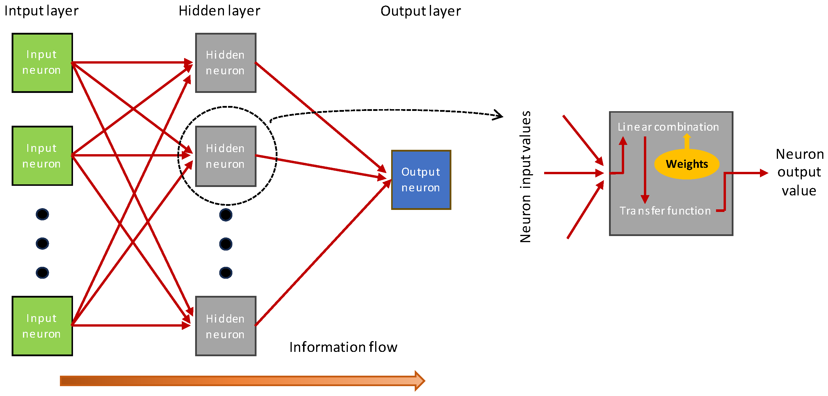
Figure 4.
Discontinuities structural parameters.
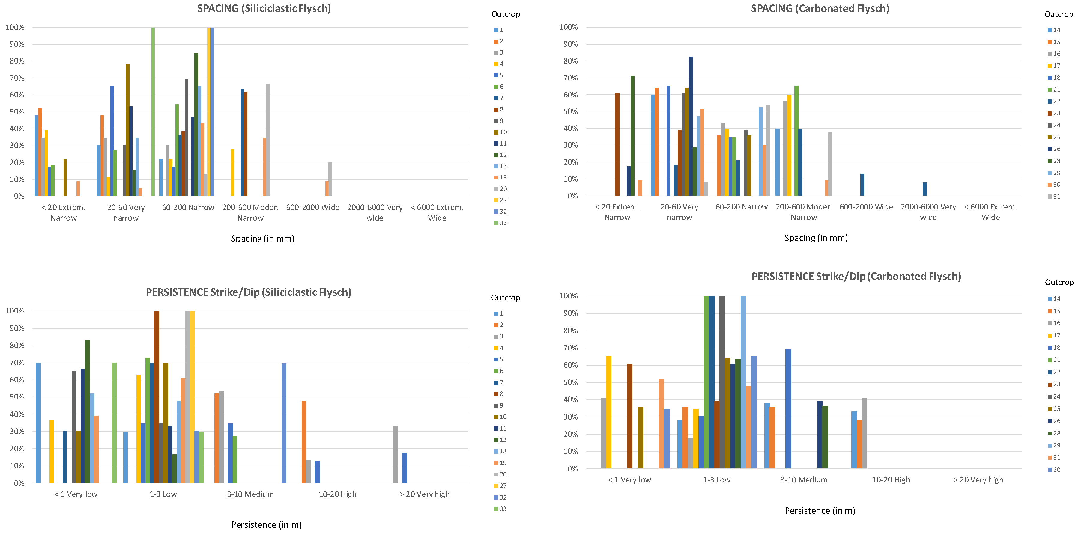
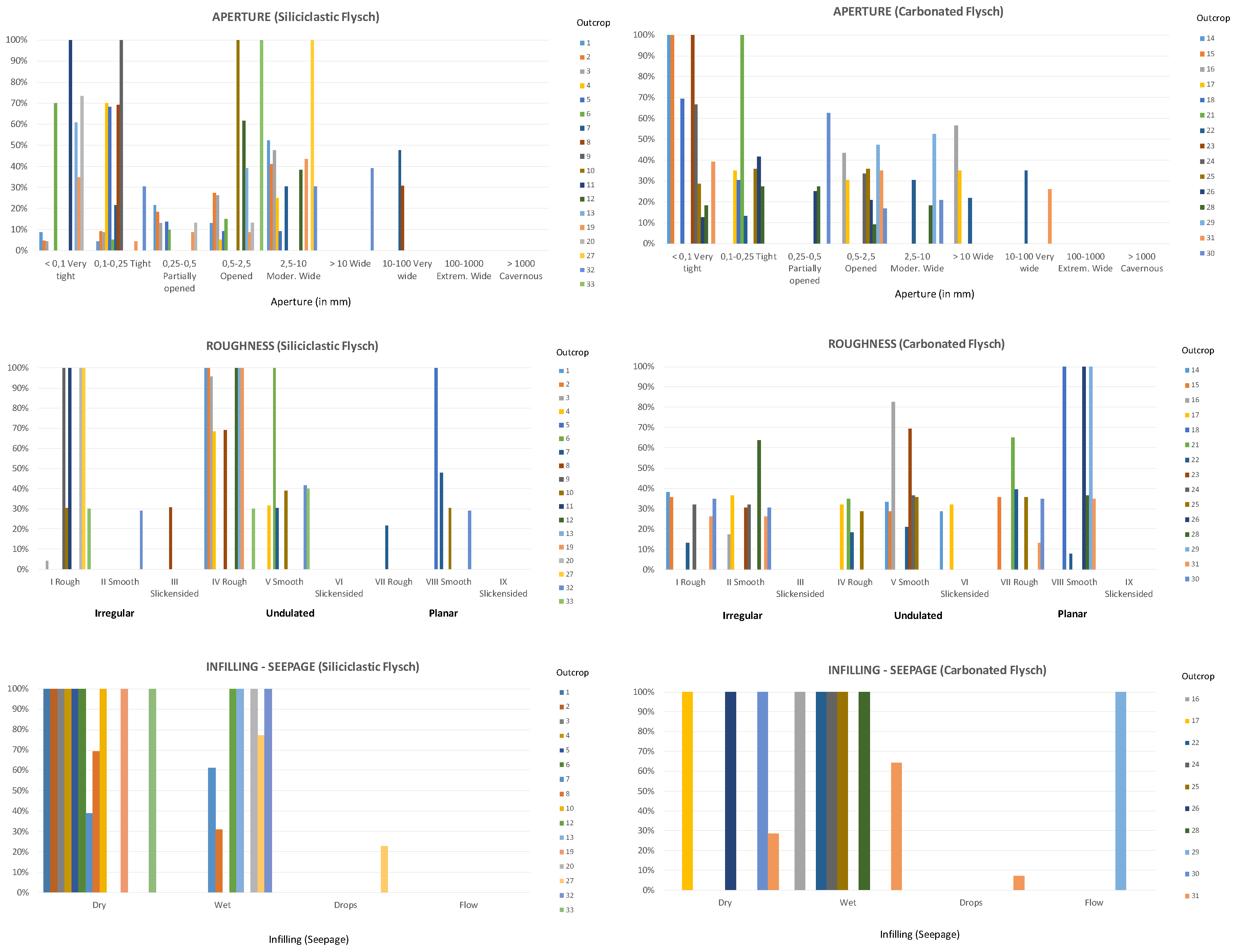
Figure 5.
Performance of the estimation of GSI values for the best AI models developed.
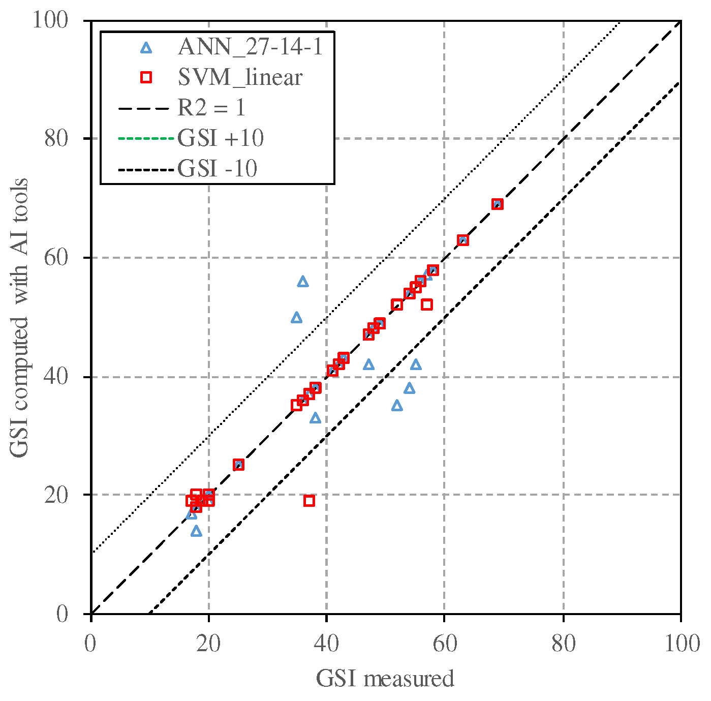

Table 1.
Results of the geomechanical tests.
| Point | Geological flysch unit | σci (MPa) | RQD | RMR | GSI | Point | Geological flysch unit | σci (MPa) | RQD | RMR | GSI | |
|---|---|---|---|---|---|---|---|---|---|---|---|---|
| 1 | Siliciclastic | 37.7 | 50 | 60 | 54 | 18 | Calcareous | 27.4 | 45 | 41 | 36 | |
| 2 | Siliciclastic | 42.4 | 45 | 62 | 55 | 19 | Siliciclastic | 50.2 | 70 | 74 | 69 | |
| 3 | Siliciclastic | 40.0 | 55 | 57 | 52 | 20 | Siliciclastic | 51.3 | 77 | 74 | 69 | |
| 4 | Siliciclastic | 42.3 | 65 | 61 | 48 | 21 | Calcareous | 25.6 | 26 | 23 | 20 | |
| 5 | Siliciclastic | 38.6 | 63 | 64 | 47 | 22 | Calcareous | 30.1 | 18 | 26 | 18 | |
| 6 | Siliciclastic | 40.1 | 65 | 47 | 35 | 23 | Calcareous | 31.0 | 43 | 49 | 41 | |
| 7 | Siliciclastic | 41.1 | 54 | 58 | 43 | 24 | Calcareous | 30.5 | 65 | 62 | 54 | |
| 8 | Siliciclastic | 32.5 | 48 | 59 | 38 | 25 | Calcareous | 17.5 | 29 | 37 | 19 | |
| 9 | Siliciclastic | 42.5 | 72 | 69 | 58 | 26 | Calcareous | 12.3 | 36 | 45 | 38 | |
| 10 | Siliciclastic | 43.2 | 69 | 72 | 63 | 27 | Siliciclastic | 13.4 | 60 | 66 | 58 | |
| 11 | Siliciclastic | 26.5 | 64 | 60 | 49 | 28 | Calcareous | 20.5 | 24 | 23 | 17 | |
| 12 | Siliciclastic | 32.1 | 63 | 55 | 47 | 29 | Calcareous | 20.0 | 25 | 44 | 37 | |
| 13 | Siliciclastic | 37.8 | 53 | 45 | 38 | 30 | Calcareous | 19.8 | 39 | 45 | 36 | |
| 14 | Calcareous | 23.5 | 20 | 43 | 37 | 31 | Calcareous | 23.4 | 32 | 47 | 42 | |
| 15 | Calcareous | 21.5 | 21 | 27 | 20 | 32 | Siliciclastic | 22.6 | 55 | 62 | 57 | |
| 16 | Calcareous | 22.3 | 23 | 21 | 18 | 33 | Siliciclastic | 32.1 | 50 | 63 | 56 | |
| 17 | Calcareous | 30.0 | 35 | 28 | 25 |
Table 2.
Laboratory testing outcomes for the flysch geological formations.
| Geological unit | Unit weight (dry), γd (kN/m3) | Uniaxial compression strength (MPa) | Tensile strength (MPa) | Point load index, Is50 (MPa) | Triaxial test on rocks (confined compression) | Shear strength of joints φr (°) | ||
|---|---|---|---|---|---|---|---|---|
| ccu (MPa) | φcu (°) | |||||||
| Siliciclastic Flysch | Minimum | 20.7 | 0.14 | 0.04 | 1.24 | 0.2 | 35 | 18 |
| Maximum | 28.5 | 76.25 | 12.47 | 4.38 | 19.9 | 44 | 30 | |
| Average | 26.4 | 24.83 | 8.43 | 2.95 | 10.0 | 40 | 23 | |
| Std. dev. | 1.4 | 18.08 | 3.56 | 1.30 | 13.9 | 6 | 10 | |
| Calcareous Flysch | Minimum | 24.5 | 6.03 | 4.55 | 0.91 | 0.2 | 42 | 23 |
| Maximum | 27.6 | 49.87 | 9.83 | 4.55 | 16.9 | 57 | 37 | |
| Average | 26.4 | 22.89 | 6.49 | 2.74 | 8.6 | 49 | 30 | |
| Std. dev. | 0.9 | 14.10 | 2.40 | 1.76 | 11.3 | 3 | 12 | |
Table 3.
Best performance at testing of ANN and SVM models developed.
| AI Model | MSE * | R2 | Ratio GSIIA / GSIfield | ||
|---|---|---|---|---|---|
| Average | Maximum | Minimum | |||
| ANN_27-5-1 | 224 | 0.79 | 0.85 | 1.47 | -0.35 |
| ANN_27-6-1 | 558 | 0.80 | 0.48 | 0.95 | -1.88 |
| ANN_27-7-1 | 91 | 0.70 | 1.22 | 1.83 | 0.87 |
| ANN_27-8-1 | 571 | 0.80 | 0.93 | 1.76 | -1.12 |
| ANN_27-9-1 | 84 | 0.74 | 1.13 | 1.54 | 0.71 |
| ANN_27-10-1 | 265 | 0.62 | 0.79 | 1.54 | -0.17 |
| ANN_27-11-1 | 98 | 0.72 | 1.27 | 2.26 | 0.79 |
| ANN_27-12-1 | 147 | 0.88 | 0.69 | 1.11 | -0.59 |
| ANN_27-13-1 | 225 | 0.74 | 0.72 | 1.19 | 0.25 |
| ANN_27-14-1 | 115 | 0.91 | 1.23 | 1.66 | 1.02 |
| ANN_27-15-1 | 253 | 0.73 | 1.29 | 2.50 | 0.39 |
| ANN_27-16-1 | 419 | 0.76 | 0.74 | 1.54 | -1.77 |
| ANN_27-17-1 | 82 | 0.75 | 1.00 | 1.29 | 0.20 |
| ANN_27-18-1 | 167 | 0.73 | 0.86 | 1.21 | -0.29 |
| ANN_27-19-1 | 115 | 0.75 | 0.97 | 1.43 | 0.22 |
| ANN_27-20-1 | 173 | 0.70 | 0.84 | 1.40 | -0.77 |
| ANN_27-21-1 | 630 | 0.62 | 0.52 | 1.14 | -0.25 |
| ANN_27-22-1 | 736 | 0.68 | 0.27 | 0.86 | -0.66 |
| ANN_27-23-1 | 96 | 0.81 | 1.03 | 1.46 | 0.59 |
| ANN_27-24-1 | 156 | 0.77 | 0.76 | 1.14 | 0.19 |
| ANN_27-25-1 | 250 | 0.77 | 1.24 | 2.03 | 0.74 |
| SVM_linear | 51 | 0.88 | 0.94 | 1.12 | 0.51 |
| SVM_radial | 182 | 0.70 | 1.35 | 1.85 | 0.93 |
* MSE considers real GSI values, which are found between 0 and 100.
Disclaimer/Publisher’s Note: The statements, opinions and data contained in all publications are solely those of the individual author(s) and contributor(s) and not of MDPI and/or the editor(s). MDPI and/or the editor(s) disclaim responsibility for any injury to people or property resulting from any ideas, methods, instructions or products referred to in the content. |
© 2023 by the authors. Licensee MDPI, Basel, Switzerland. This article is an open access article distributed under the terms and conditions of the Creative Commons Attribution (CC BY) license (http://creativecommons.org/licenses/by/4.0/).
Copyright: This open access article is published under a Creative Commons CC BY 4.0 license, which permit the free download, distribution, and reuse, provided that the author and preprint are cited in any reuse.


