Submitted:
12 December 2023
Posted:
14 December 2023
You are already at the latest version
Abstract
This paper focuses on improving the tracking accuracy for servo systems and increasing the contouring performance of precision machining. The dynamic friction during precision machining is analyzed using the LuGre model. The dynamic and static parameters in the friction model are efficiently and accurately identified using the improved Drosophila Swarm Algorithm based on cross-mutation. The friction tracking error can be deduced by the friction state space and an expression is derived. To compensate for the tracking error caused by friction, a feedforward compensation control is designed to avoid signal lag in traditional friction controllers. Furthermore, the factors of multi-axis parameter mismatching that impact the machining profile accuracy are analyzed for multi-axis control. An adaptive cross-coupled control-based pre-compensation strategy of contour error is designed to reduce both the tracking error and the contour error. The effectiveness of the proposed method is validated through several experiments, which demonstrate a remarkable improvement in tracking performance and contour accuracy.
Keywords:
Friction force prediction
; feed-forward control
; multi-parameters identification
1. Introduction
Tracking error is an important evaluation index for measuring the single-axis motion accuracy of a precision machining platform [1-5]. It describes the difference between the actual position and the command position, which hinders the machine tool from moving to the specified position accurately and leads to contour errors in multi-axis linkage [6-7]. Traditionally, methods for correcting tracking errors involve detecting the absolute position of the actuator. Although this method can reduce tracking error to some extent, it fails to meet the high precision requirements of precision machining [8-9]. Therefore, it is necessary to analyze the tracking error in detail and design advanced control strategies to compensate for it. In the process of precision machining, internal factors such as servo delay, friction, thrust fluctuation, and vibration, as well as external factors like assembly, wear, and temperature, can all influence tracking error [10-11]. This paper focuses on internal friction disturbance, analyzes its influence on tracking error, and establishes an estimation model and control strategy. Additionally, the paper thoroughly examines contour error modeling and design strategies for control.
Friction, caused by the contact of surfaces within each mechanism, hinders the linear feeding motion of a machine tool and reduces the output accuracy and motor motion stability of the machining process. This is particularly problematic for parts with high surface quality requirements since friction disturbance can disrupt the continuity and integrity of the workpiece surface, resulting in increased RA and RMS roughness values [12]. Existing research categorizes friction into two main types: static friction and dynamic friction [13-14]. Several static models have been developed, including the Coulomb force model [15], the static friction viscous damping model [16], Stribeck model [17], and Karnopp model. However, these models have limitations in fully capturing the nonlinear dynamic characteristics of pre-sliding friction, static friction, and lag friction. On the other hand, dynamic friction models such as the LuGre model [18], Leuven model [19], and Maxwell slip model [20], are widely used due to their simple structure and strong dissipation. The LuGre model decomposes the friction process into pre-sliding and sliding stages, allowing for a comprehensive description of the static and dynamic characteristics of friction. It effectively addresses the limitations of the static friction model. However, accurate identification of static and dynamic parameters is crucial in LuGre friction modeling. Liu proposed a distributed decoupling identification method to separate the friction characteristics of the pre-sliding and sliding stages, enabling separate identification and compensation for each stage [21]. Differential evolution identification algorithms are used to accurately obtain the friction model parameters, reducing computational complexity, and ensuring global optimization performance [22]. Seung Jean proposed an autoregressive model to identify the coefficient of viscous friction in the frequency domain [23]. Furthermore, various algorithms such as trained neural networks, least square methods, genetic algorithms, and ant colony algorithms are utilized for friction parameter identification [24-25]. However, these algorithms mostly focus on single parameter identification and have low efficiency for multi-objective parameter identification.
By using the control strategy to predict and compensate for the error caused by friction, the machining accuracy of precision machine tools can be effectively improved. Firstly, friction modeling and parameter identification can be carried out for the machine tool, and embedded into the system by friction feed-forward control. The control strategy compensates for the friction torque estimated by state variables. To observe the state variables, Truong's double observers are utilized to predict the nonlinear state variables in the friction process. This is combined with the advanced sliding mode adaptive control to achieve the friction compensation of the linear servo system [26]. Lin proposed an adaptive robust controller that modifies the LuGre model and incorporates a nonlinear observer to estimate the friction torque [27]. Iwasaki proposed a LuGre friction disturbance observer that includes both the static and dynamic characteristics of friction to accurately simulate the actual machining. Experimental results demonstrate that this method significantly improves the motion tracking performance of the system [28]. Rafan, using a feedforward PID compensator, takes advantage of the static friction model and generalized Maxwell model to compensate for friction in both the sliding and pre-sliding stages, resulting in a certain degree of improvement in trajectory tracking accuracy [29].
To improve the contour accuracy of precision machining, traditional methods focus mainly on reducing single axis tracking errors to decrease contour errors in the whole system. However, these methods have limited effectiveness due to their lack of consideration for the coupling of multi-axis linkage. Additionally, the contour compensation values for each axis lack coordination and adaptability. To address this issue, a cross-coupled compensation strategy is implemented, which considers the parameter diversity and matching of each axis, and adjusts the contour error compensation signal comprehensively. Furthermore, the contour error compensation is proportionally returned to each axis based on their motion characteristics. Compared to direct symmetrical compensation, the cross-coupled control (CCC) method is more accurate [30] and has a more significant impact on improving machining contour accuracy [31-32].
The organization of this paper is as follows. Section 2 introduces the modeling of tracking error and friction force, and deduces the control strategy for friction. Section 3 focuses on the modeling of contour error and the design of the cross-coupled control strategy. In Section 4, an experimental analysis is performed and the results are compared. Finally, Section 5 presents the conclusion.
2. Modeling and identification of friction
The U-type linear motor is regarded as the driving source of the precision platform. It improves transmission efficiency and reduces friction loss by eliminating the complicated mechanical transmission structure. However, the friction between the slider, platform, and other surface contact links cannot be completely avoided. This friction, influenced by factors such as load and weight, hinders the feed motion of the machine tool. Particularly at low speeds and during reversing, position deviations increase significantly, leading to a decrease in overall machining accuracy. Additionally, excessive friction impacts the stability of motor thrust output. Therefore, this section analyzes the friction disturbance and tracking error caused by the friction of the linear motor.
2.1. LuGre friction modeling
LuGre model is widely used in friction identification due to its ability to absorb the Stribeck effect and accurately describe friction characteristics through bristle parameters. The process of precision machining involves a variety of mixed nonlinear states that can cause friction disturbances. LuGre model is described as follows:
Where is average deformation of bristle, is relative feedrate, is the Stribeck speed. are friction force, Coulomb force, and maximum static friction respectively. are sideburns stiffness, damping coefficient and friction coefficient respectively. is the Stribeck function.
In the movement of a precision linear mechanism, the sliding friction is changed with different feedrates, resulting in inconsistent surface roughness that increases the calculation difficulty of friction. The dynamic parameters and static parameters are used to exhaustively describe the friction force in this complex movement. However, due to the bilateral symmetrical structure of the U-type linear motor, this paper does not consider the influence of the normal force on the friction force. Moreover, the normal thrust fluctuation between the primary and secondary can be offset, making it negligible.
Substituting (2) into the LuGre model
Eq. (3) contains the state variable , which can describe the friction process more comprehensively. The accuracy of parameters directly affects the accuracy of friction modeling. Therefore, the identification parameter matrix is established, and the variance of deviation degree between the actual path and the reference path is regarded as the evaluation function
2.2. Multi-parameter identification of friction model
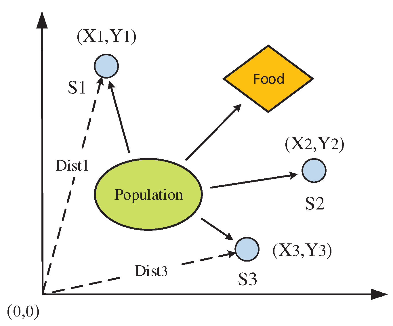
The parameters of the LuGre model can be accurately identified by addressing the limitations of conventional iterative algorithms, as shown in Eq. (4). However, these algorithms struggle to yield satisfactory results for the multi-parameters synchronous identification. To overcome these challenges, a new fly optimization algorithm (FOA) is proposed. The FOA enables group optimization, making it suitable for identifying the parameters of the LuGre model. By employing dynamic step and adaptive cross mutation, the FOA effectively addresses the issue of the traditional Drosophila algorithm falling into local extremum, thereby improving the accuracy of parameter identification. The FOA mimics the predatory process of drosophila, utilizing its olfactory superiority to quickly distinguish complex odors in the air. FOA stands out from other optimization algorithms due to its simplicity in structure, ease of programming, faster convergence, and fewer parameters. The foraging process of FOA is depicted in Figure 1.
Figure 1.
Iterative foraging process of fruit flies.
The adaptive crossover factor is introduced to regulate the crossover of the population to search for the global optimal value of the population. This effectively improves the adaptability of the Drosophila individual to environmental changes. The main steps involve randomly pairing the Drosophila population and selecting any pair as the parent. After crossover and mutation, the same number of offspring is generated as the parent. The cross-mutation process enhances the population diversity and the ability to jump out of local extremum.
The fitness of the N-th population of drosophila can be expressed as . The crossover probability q and is shown as follows:
are range of crossover probability, Smellmid represents the larger fitness value of two cross particles, Smellmax is the maximum fitness in population and Smellavg is the average value in population.
To maintain a certain crossover probability and obtain more excellent genetic genes, the function of constant Acon is used to slow down the variation trend of crossover probability q when the fitness value is high. This ensures the number of excellent offspring and improves the heritability of dominant genes (5) ~ (7). Therefore, the drosophila population, which is close to the highest quality part of the whole world, can benefit from maintaining a certain crossover probability and acquiring more excellent genetic genes. As shown in Figure 2, the parameter identification process of LuGre modeling using the improved drosophila algorithm is as follows:
(1) The calculation of the determination value of concentration S requires the initial pop ulation parameters, such as population size, the number of iterations (tmax), initial positions (X_pos and Y_ pos), fitness threshold (δ), search radius (Rvalue), mutation probability (q), and search direction.
To enhance both global search efficiency and local search accuracy, the proposed approach incorporates the strategy of dynamically reducing step length. Initially, a larger step length is employed to facilitate a wide range search of the entire population, enabling quick identification of the target area. As the target area is approached, the search step length and speed are gradually decreased to encourage the drosophila particles to explore the vicinity of the optimal solution in depth. Simultaneously, the issue of the population being prone to getting trapped in local minima is addressed through the utilization of an exponential distribution function. The improved formula is as follows:
Where Smellbesti-1 is the last generation optimal flavor concentration value, Lmax is the maximum step length, α=0.01 is the exponential factor, ti is the current iterations and Ri is the exponential distribution function that the power exponent is 0.5.
(2) The paragraph calculates the average taste concentration (Smellavg), and the variance in taste concentration (). A smaller variance indicates a higher concentration and lower diversity within the population.
Figure 2.
Iterative foraging process of fruit flies.
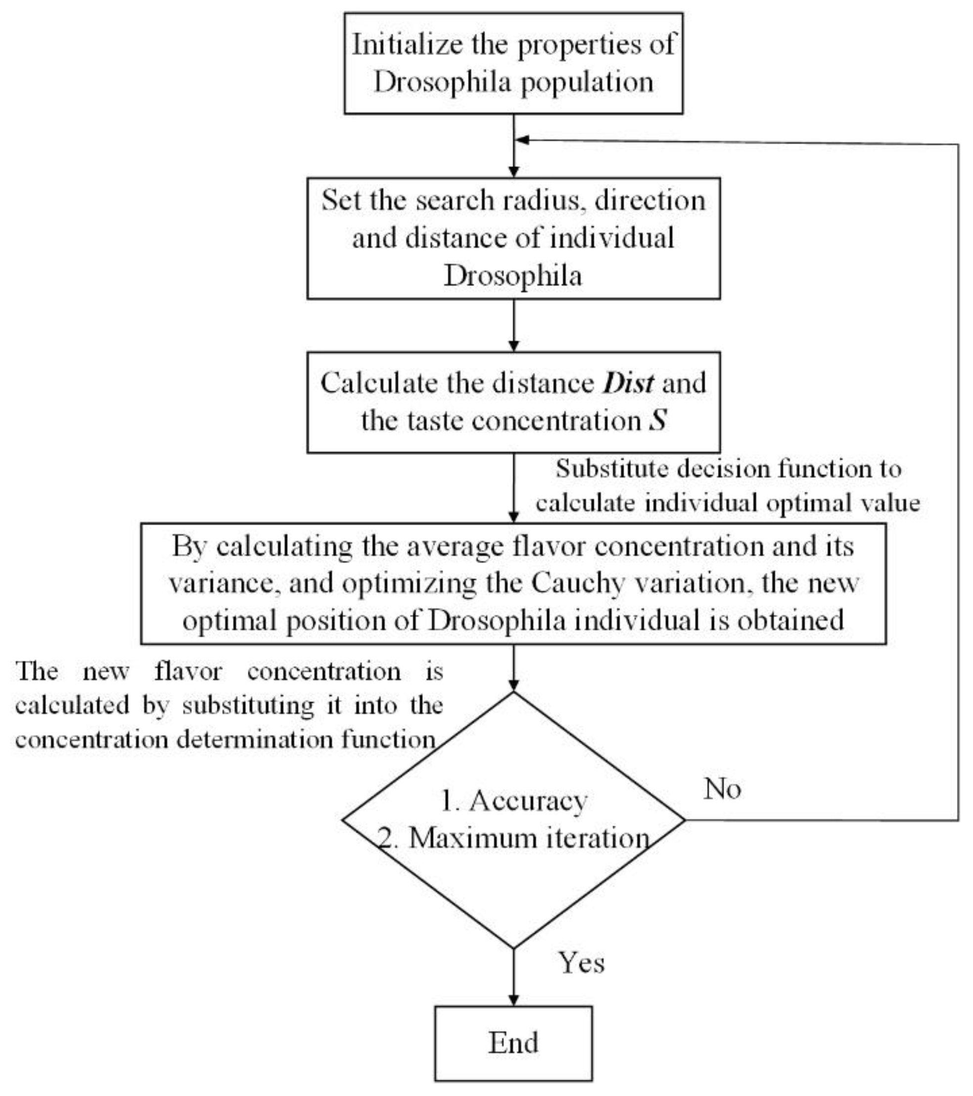
When the current fitness value Smellbest does not reach the target requirement and σ^2≤δ, it can be inferred that the current population is trapped in a local extremum. In this case, if the random number (0~1) is less than the mutation probability q, the optimal positions undergo Cauchy mutation for optimization. Subsequently, the new optimal positions of the drosophila individuals are obtained through secondary optimization of the mutated particles.
(3) Re-estimate the distance between the new position, the origin and the determination value of concentration.
Substituting into taste concentration function and calculating the new taste concentration.
If , then ,,. The flowchart shown in Figure 2 represents the iterative process described above, which is repeated until either the maximum number of iterations is reached or the desired level of accuracy is achieved. This process incorporates the adaptive crossover of drosophila, which helps to make the distribution of individuals more realistic during the optimization process. Additionally, the inclusion of a threshold and the implementation of Cauchy mutation serve to enhance the overall diversity of the population, addressing the issue of particles becoming prematurely trapped in local optima.
The advantages of the improved drosophila algorithm are demonstrated through the iterative evolution curve shown in Figure 3 and the parameter identification results displayed in Table 1. Figure 3 reveals that the improved drosophila algorithm exhibits faster convergence speed and higher efficiency. To further highlight these advantages, three traditional algorithms are compared. As demonstrated in Tab.1, the identification algorithm proposed in this paper achieves higher accuracy, with the maximum error being only 0.96%. This method is more suitable for the multi-parameter synchronous identification of the LuGre model compared to traditional iterative algorithms. Finally, the identified LuGre parameters are utilized to calculate friction and fit the friction feed rate curve, as depicted in Figure 4.
Figure 3.
Iterative foraging process of fruit flies.
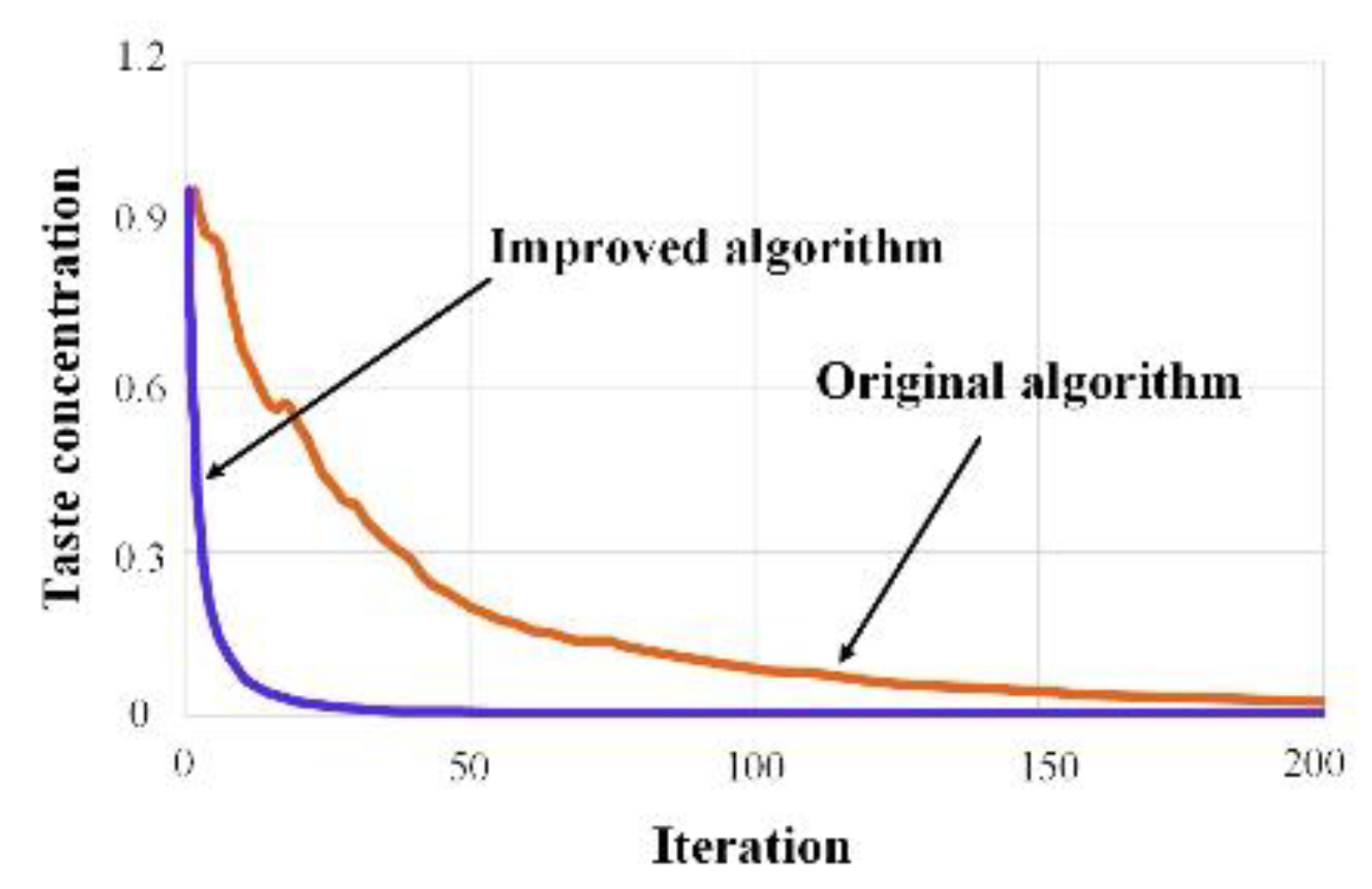
Figure 4.
Relationship diagram of friction and velocity.
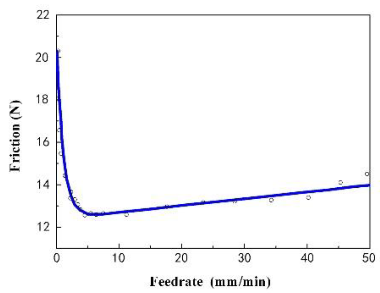

Table 1.
Identification results of friction parameters.
| Design values | Least square method | Genetic algorithm | Ant colony algorithm | Proposed algorithm |
|
| (N) | 30.00 | 30.51 | 30.63 | 30.21 | 30.12 |
| (rad/s) | 0.500 | 0.479 | 0.485 | 0.490 | 0.498 |
| (Nm/s) | 560.0 | 549.4 | 554.1 | 556.7 | 550.6 |
| (Nm/s) | 300.0 | 291.0 | 294.2 | 303 | 299.8 |
2.3. Tracking error modeling
To improve the overall contour machining accuracy of the PMLSM, it is crucial to address the issue of deviation between the actual position and theoretical position caused by friction. The complex curvature trajectory often results in sliding and crawling, which exacerbates the problem. Analyzing the tracking error attributable to friction offers an opportunity to enhance the increment accuracy of the PMLSM. Taking X-axis for an example, the system state space expression is shown as
Substituting (16) into (1), the state equations can be expressed as
where .
m —— mass matrix
c1 —— equivalent viscosity coefficient
K —— Stiffness coefficient
—— thrust coefficient
—— amplifier gain
—— input control
d —— disturbance.
Supposing the theoretical position is , the feed error is , the acceleration deviation is
Thus, the tracking error can be obtained by solving the differential equation with the given error state space expression.
3. Friction compensation and control strategy
3.1. Friction feed-forward control design
The problem of error compensated signal has been a major obstacle in the traditional method of controlling the motion accuracy of linear motors through feedback. To overcome this difficulty and improve precision machining, a feed-forward control compensator strategy has been designed. This strategy estimates and adjusts the tracking error caused by friction before it is input into the motor, thus avoiding cycle delay and improving the motion tracking accuracy of a single axis. To illustrate this strategy, a schematic diagram of the X-axis is shown in Figure 5.
Figure 5.
Friction compensation model.
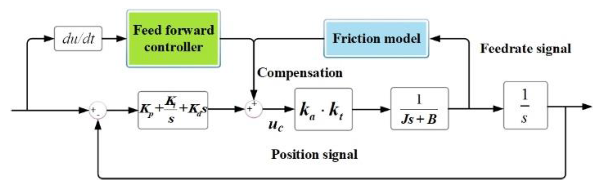
The simulation structure diagram of the LuGre model, shown in Figure 6, utilizes the velocity feedback as input to calculate the parameters. To estimate the friction force, the average elastic deformation is obtained through simulation since the bristle z, being an intermediate state variable, cannot be accurately determined. The position tracking accuracy control performance of the linear motor is improved by superimposing the tracking error compensation, adjusted by feedforward control, with the theoretical data. Furthermore, Figure 7 illustrates the simulation block diagram of the friction feedforward controller.
Shown in Figure 8, the comparison of simulated results for friction compensation reveals that the feedforward compensation strategy effectively mitigates friction disturbance during linear motion. The maximum friction is reduced by over 50%, and the fluctuation of friction compensation remains stable. Consequently, it is evident that this control strategy enhances the tracking performance of linear motors and improves the contour accuracy of precision machining.
3.2. Experiment of friction compensation control
The effectiveness and necessity of friction feed-forward control are verified by comparing the tracking error before and after friction compensation control. The friction feed-forward control is tested using the experiment of complex curves on the precision machining platform, as shown in Figure 9. The experimental path consists of straight lines and curves, with a total length of 600mm and a feed rate of 500mm/min. Since friction hinders the motion of the linear motor, it results in a reduction of tracking accuracy. Therefore, the tracking error is considered as the index for friction compensation.
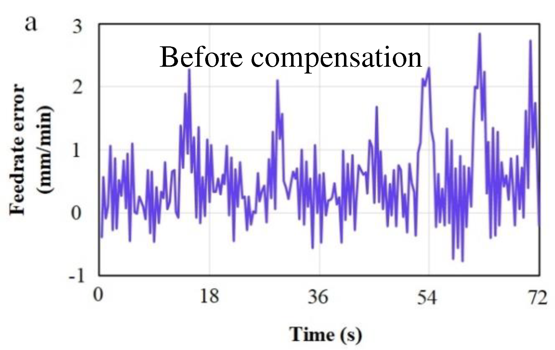
The comparison results of the tracking error are shown in Figure10. The original tracking errors for the X-axis and Z-axis are represented by a and d, respectively. The tracking errors for the X-axis and Z-axis using the traditional friction compensation strategy are denoted by b and e, while the tracking errors with the feed-forward compensation strategy are represented by c and f. The maximum tracking errors for the X-axis under the three strategies are 3.98 μm, 3.32 μm, and 3.13 μm. Meanwhile, for the Z-axis, the maximum tracking errors are -3.71 μm, -3.25 μm, and -2.78 μm. The proposed feedforward control strategy outperforms the traditional method in terms of compensation performance. The maximum tracking accuracy can be improved by 25.1% at the sharp corner.
The research of friction disturbance can enrich the analysis of motion tracking accuracy of linear motor. In addition, friction can also influence the feedrate. This deviation can be reduced by feedforward control compensation. Figure 10 shows that the feedrate errors have been improved from 2.8 mm/min to 2.3 mm/min (17.8%). Furthermore, the friction feedforward compensation strategy enhances the tracking accuracy, thus providing a foundation for improving the overall machining contour accuracy of the precision machining platform.
4. Contour error modeling and controlling
4.1. Contour error modeling
In the Figure 11, the contour error can be defined as where is the nearest point from the actual point on the designed trajectory to the actual point. To calculate the contour error, the proximate point Pe is used to instead of to calculate the contour error. Therefore, is replaced by an estimated contour error .
As shown in the Figure 11, the unit orthogonal tangent vector t and normal vector n and bi-normal vector vectors along with reference path are computed by
and the Frenet Frame consists of the three vectors, . Then, the tracking error e is transformed into the Frenet Frame
Finally, the delay timetd of contour error is
In order to calculate the Pe using Taylor expansion, the delay displacement and estimated contour error are determined. It is worth noting that both and lie on the reference path, implying that the modeling accuracy is higher than that of the traditional method, where the estimated point often deviates from the design trajectory.
4.2. Influence of the dynamic parameter on contour error
In this section, the influence of the inertia of each axis parameter on the contour error will be discussed. As mentioned above, improving the single axis tracking accuracy alone may not significantly improve the contour accuracy. This is mainly because the contour error is caused by the uncoordinated motion of each axis and the differences in inertia between them, making it difficult to directly compensate for the contour error. In the system, the input and output have the following relationship
Where is the motion period constant, is the actual trajectory, is the designed trajectory and is the close loop gain. Taking the shell parts as an example on the precision machining platform, when the radius of circular trajectory is R
Substituting into (24), the steady-state solution of the system can be expressed as
For shell parts, the deviation between the actual trajectory and the designed path can be expressed as
With steady state expansion and ignoring the higher order polynomials, then equation (25) can be rewritten as
where;
As we can see in Eq. (27), er is mainly affected by the inertia parameters of each axis system in the second and third items, the details are shown as follows
- (1)
- When the motion time and dynamic gains of each axis are equal, the second and third terms of equation (27) become zero. Consequently, the error er is solely influenced by the first servo dynamic characteristics. In this scenario, the error is dependent on both the frequency of the servo bandwidth and the size of the design path.
- (2)
- When the motion time constants Tx and Ty of each axis are different, but the motion gains Kcx and Kcy are the same, the Eq. (27) can be rewritten as
- (3)
- Except for the first item, error er is affected by two parts based on (28). One part is constant and independent of time. The other part consists of elliptic trajectories that vary with time. These trajectories have a major axis distributed in the direction of 45° or 135°, and their radius is related to the system dynamic parameter ωt.
- (4)
- When the motion time constants Tx and Ty are equal, but the motion gains Kcx and Kcy are different, equation (27) can be rewritten as follows
In this case, the error er can be compared to the second case, where the error curve resembles an ellipse. The major and minor axes of this ellipse are correlated with the radius of the intended path.
- (5)
- When Tx, Ty and Kcx, Kcy are all different, Eq. (28) can be rewritten as
Eq. (30) shows the relationship between the error er and the parameters of each axis, and the trend of er is similar to the second and third cases.
From the above analysis, it can be observed that the contour error of a linear servo system is influenced by several factors. These include the command signal frequency, the curvature of the designed path, the system frequency response, and the motion dynamic gain of each axis. Merely enhancing the tracking accuracy of a single axis does not effectively reduce the overall contour error. Therefore, it is crucial to consider the problem of inertia matching and error compensation coordination of each axis.
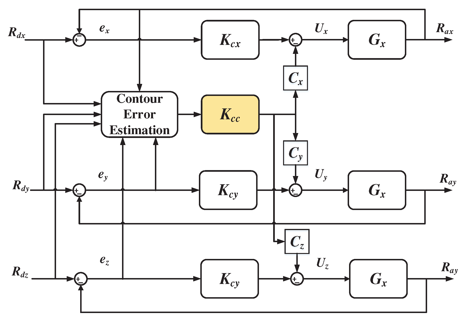
4.3. Design of cross-coupled control strategy
In this section, a three-axis cross-coupled controller is designed to adjust and control the estimated contour error. The central controller, represented by and consisting of a Fuzzy PID controller, plays a crucial role in the entire CCC system as it determines the accuracy of compensation. Kci and Gi(i=x, y, z)are the position controller and controlled object respectively. The estimated contour error, as shown in Figure 12, is input into the central controller, which generates an error control signal by coupling it with the parameters of each axis. The compensation of the contour error is then decoupled to each axis in proportion and superimposed with the theoretical point . This process enables the prediction and compensation of the contour error. The actual position , meanwhile, serves as a reference for comparison. To facilitate the controller design and ensure consistency, the motion cycle parameters of each axis are set to the same value, .
Firstly, it is assumed that the contour error is when cross-coupled controller is not added, that is to say , as known in Figure 12, where Kci and Gi(i=x, y, z)are position controller and the controlled object. When the CCC is adopted, the contour error can be expressed as
Figure 12.
Central controller of cross-coupled controller.

Figure 13.
B-spline complex spline path.
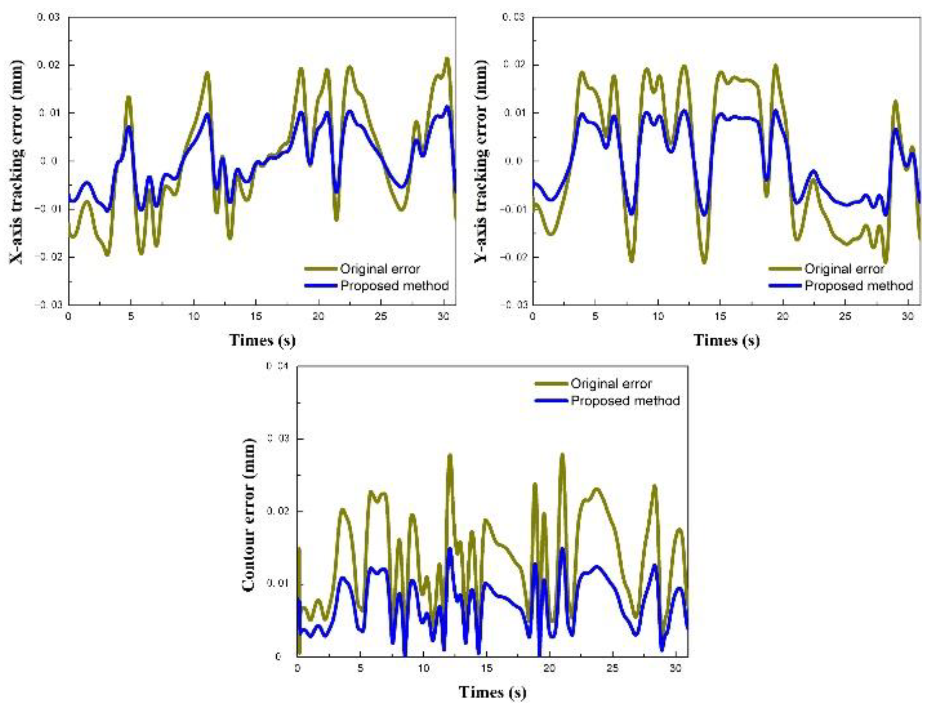
In actual machining, the main factor that affects contour accuracy is the mismatch of parameters in multi-axis. This mismatch leads to an uneven distribution of contour error throughout the whole trajectory. To address this issue, a pre-compensation strategy is proposed. The strategy takes advantage of the curvature variation characteristics of the spline path to reduce the contour error. Additionally, it considers the inertia matching and coordination of the parameters in each axis to improve the machining contour accuracy. A complex B-spline path of simulation, with a total length of 742 mm and a feed rate of 1400mm/min, is shown in Figure 13. As shown in Figure 14, the maximum tracking error of the x-axis and y-axis is reduced by 47.01% and 47.02% respectively, while the contour error is reduced by 46.5%. Consequently, the proposed strategy significantly improves the contour error.
Figure 14.
Error contrastive results of pre-compensation of CCC.
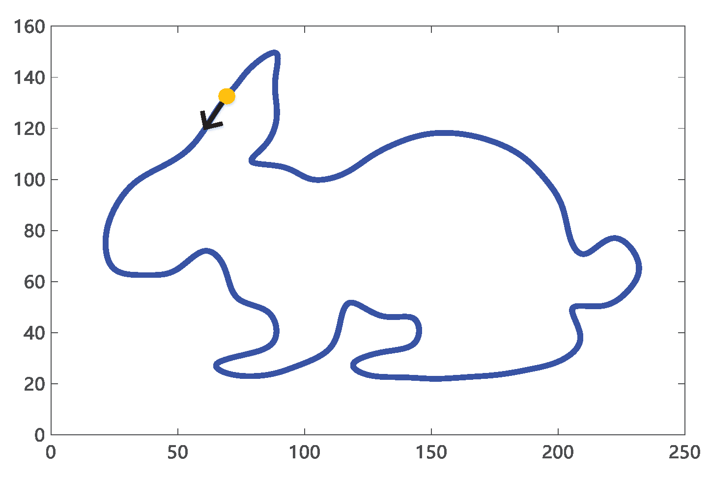
Figure 15.
Machining experiment of spherical shell.
5. Machining experiment verification
The effectiveness of the proposed friction control strategy on the precision turning and grinding integrated machining platform, shown in Figure 15, is verified by the precision machining of shell parts. The shell is made of aluminum (7075) and has a radius of 120 mm and a wall thickness of 3 mm. The machining parameters used are as follows: a speed of 450 r/min, a feedrate of 10 mm/min, and a cutting depth of 0.005 mm. The shell parts are cut using a carbide turning tool, and the cutting mode from the bottom to the top of the shell is selected to ensure machining quality and cutting integrity. In this experiment, the effect of cutting force is ignored due to the small cutting depth. During the machining process, friction hinders the feed movement of the machine tool, resulting in a reduction in tracking accuracy and overall contour accuracy of the parts. Therefore, in this section, the compensation effect of each axis tracking error is used as the standard to measure the performance of the proposed friction control strategy and to verify its effectiveness and necessity.
Figure 16.
Compensation result of tracking error.
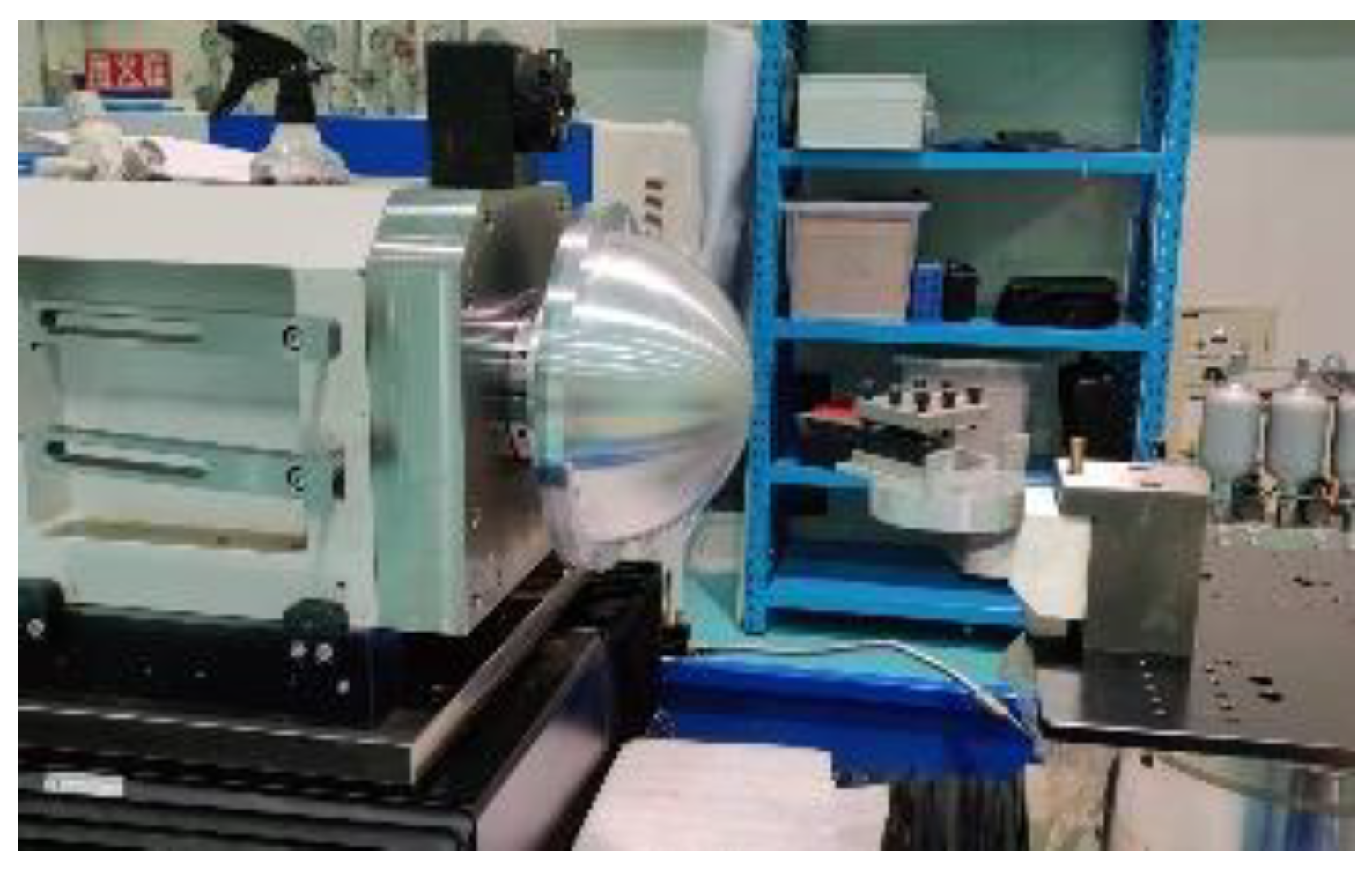
Figure 17.
Compensation result of contour error
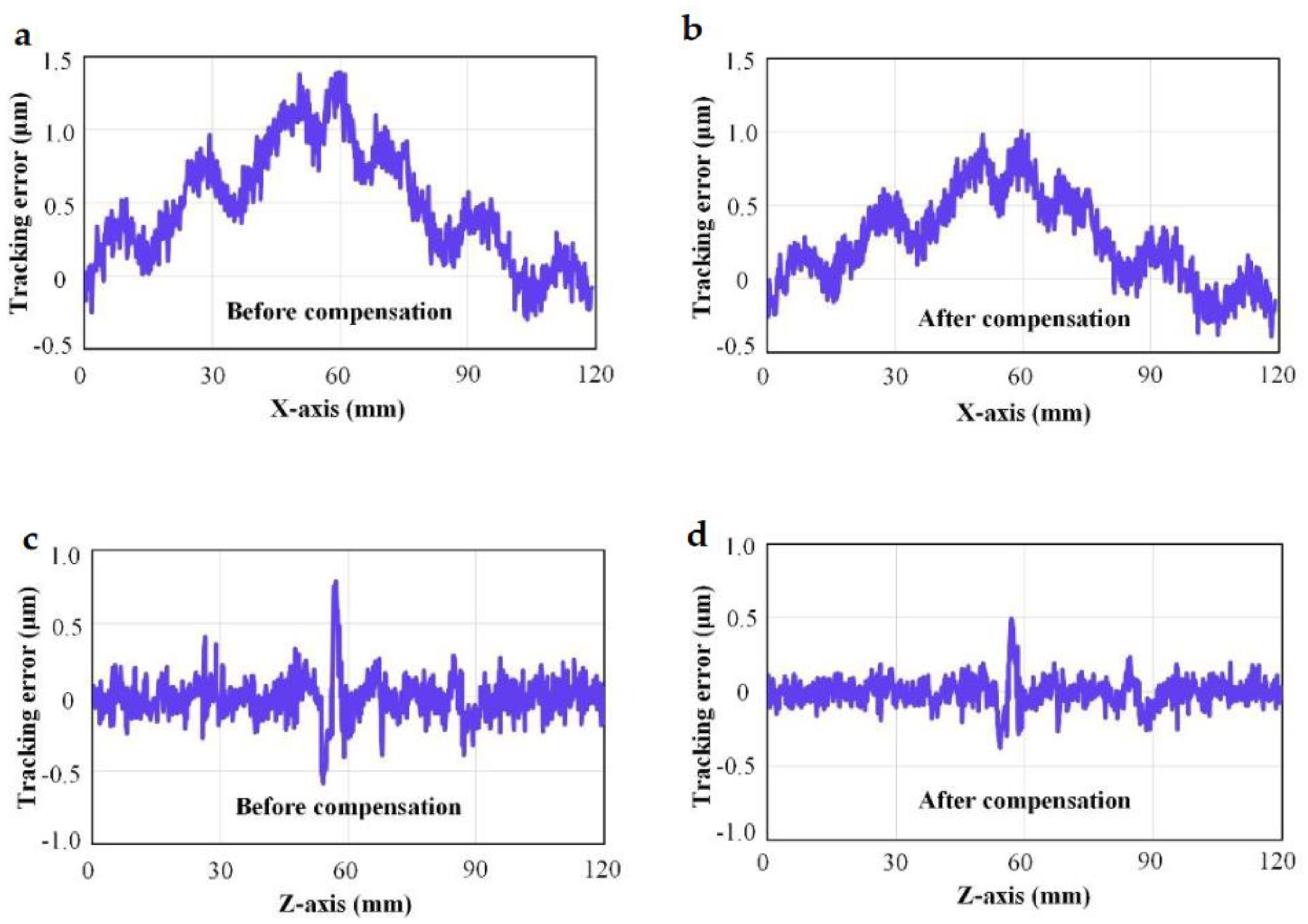
Due to dynamic friction disturbance, the motion accuracy of the linear motor decreases with high feed rate. In Figure 16, the original tracking errors of the X-axis and Z-axis are represented by a and c, respectively. Friction compensation control for the X-axis and Z-axis is denoted by b and d, respectively. The control compensation strategy based on the LuGre friction model can significantly reduce the tracking error and contour error. The thrust fluctuation causes the error to fluctuate periodically, resulting in slightly different compensation effects at different positions. As shown in Figure 16 and Figure 17, the tracking error is reduced from 1.41 μm and 0.81 μm to 1.02 μm and 0.50 μm, respectively. In addition, the contour accuracy is improved from 1.81 μm to 1.43 μm. The friction control compensation strategy further refines the motion analysis of the linear motor, improves tracking accuracy, and lays the foundation for enhancing the overall contour accuracy of the precision machining platform.
6. Conclusions
To improve the machining accuracy in precision machining, several strategies are employed. Firstly, the LuGre model is utilized for dynamic friction modeling, with the dynamic and static parameters accurately identified using the improved Drosophila multi-objective parameters optimization algorithm. Through state space analysis, the expression of tracking error caused by friction is derived. Additionally, a feed-forward compensation strategy is implemented to address the periodic signal delay issue present in traditional friction control models. Secondly, a pre-compensated cross-coupled control strategy is designed to regulate and distribute compensative values to each axis. This strategy takes into account the mismatch problem arising from the inertia parameters of each axis, ensuring accurate control over the contour error. Experimental results indicate that this friction compensation strategy can reduce the tracking error by up to 25.1%, thereby guaranteeing precise motion control of the machine tool under extreme conditions.
Author Contributions
Jiqiang Yu: Conceptualization, Validation, Formal analysis, Investigation. Zheng Zhang: Validation, Formal analysis. Weirui Liu: Writing—original draft, Project administration, Supervision, Funding acquisition. Xingjun Gao: Investigation. Ruixin Bao: Investigation.
Funding
This work was funded by the Basic Scientific Research Projects of Liaoning Provincial Department of Education (Grant No. JYTMS20231454), China Postdoctoral Science Foundation (Grant No. 2022M710833), and the College Students Innovative Entrepreneurial Training Plan Program (Grant No.202210148027).
Data Availability Statement
All the data presented in this study are contained in the article’s main text.
Conflicts of Interest
The authors declare no conflict of interest.
References
- Jiang SL, Sun YW. Stability analysis for a milling system considering multi-point-contact cross-axis mode coupling and cutter run-out effects. Mechanical Systems and Signal Processing 2020, 141, 106452. [CrossRef]
- Quynh NV. The Fuzzy PI Controller for PMSM's Speed to Track the Standard Model[J]. Mathematical Problems in Engineering, 2020, 2020. [CrossRef]
- Xu JT, Zhang DY, Sun YW. Kinematics performance oriented smoothing method to plan tool orientations for 5-axis ball-end CNC machining. International Journal of Mechanical Sciences 2019, 157-158, 293–303. [CrossRef]
- Jiang Y, Guo Q. Simulation of multi-axis grinding considering runout based on envelope theory. Chinese Journal of Aeronautics 2020, 33, 3526–3534. [CrossRef]
- Zhao DM, Gao XJ, Wang Y. Design of Piezoelectric Ceramic Pliable Microgripper Based on Two Flexible Hinges. Journal of Liaoning Petrochemical University 2022, 42, 64–69.
- Dong H, Zhu XZ, Chen L. Analysis of Vibration Characteristic of Spindl⁃Bearing System of High Speed Grinding Machine. Journal of Liaoning Petrochemical University 2021, 41, 56–60.
- Wang S, Chen G, Cui Y. Design of Contour Error Coupling Controller Based on Neural Network Friction Compensation. Mathematical Problems in Engineering 2019. [CrossRef]
- Zhang S, Hao Q, Liu Y, et al. Simulation Study on Friction and Wear Law of Brake Pad in High-Power Disc Brake[J]. Mathematical Problems in Engineering. 2019. [CrossRef]
- Lu SK, Hua DX, Li Y, et al. Stiffness Calculation Model of Thread Connection Considering Friction Factors[J]. Mathematical Problems in Engineering, 2019, 2019:1-19.
- Sun YW, Jiang SL. Predictive modeling of chatter stability considering force-induced deformation effect in milling thin-walled parts [J]. International Journal of Machine Tools and Manufacture, 2018, 135: 38-52.
- Ding R, Xiao L. Quadratic Integral Sliding Mode Control for Nonlinear Harmonic Gear Drive Systems with Mismatched Uncertainties[J]. Mathematical Problems in Engineering, 2018, 2018(PT.9):1-18.
- Armstrong-Hélouvry B, Dupont P, Wit CCD. A survey of models, analysis tools and compensation methods for the control of machines with friction[J]. Automatica, 1994, 30(7):1083-1138.
- Simba KR, Bui BD, Msukwa MR, et al. Robust iterative learning contouring controller with disturbance observer for machine tool feed drives[J]. ISA Transactions, 2018: S0019057818300703.
- Li CB, Pavelescu D. The friction-speed relation and its influence on the critical velocity of stick-slip motion[J]. Wear, 1982, 82(3):277-289.
- Dahl, Philip R. Solid Friction Damping of Mechanical Vibrations[J]. AIAA Journal, 1976, 14(12):1675-1682.
- Canudasd WC, Olsson H, Astrom KJ, et al. A new model for control of systems with friction[J]. IEEE Transactions on Automatic Control, 1995, 40(3):419-425.
- Freidovich L, Robertsson A, Shiriaev A, et al. Friction compensation based on LuGre model[C]. IEEE Conference on Decision & Control. IEEE, 2006.
- Swevers J, Al-Bender F, Ganseman CG, et al. An integrated friction model structure with improved presliding behavior for accurate friction compensation[J]. IEEE Transactions on Automatic Control, 2000, 45(4):675-686.
- Chu H, Gao B, Gu W, et al. Low-Speed Control for Permanent-Magnet DC Torque Motor Using Observer-Based Nonlinear Triple-Step Controller[J]. IEEE Transactions on Industrial Electronics, 2017, 64(4):3286-3296.
- Cui P, Zhang D, Yang S, et al. Friction Compensation Based on Time-Delay Control and Internal Model Control for a Gimbal System in Magnetically Suspended CMG[J]. IEEE Transactions on Industrial Electronics, 2017, 64(5):3798-3807.
- Liu D, Tao T, Mei CS, et al. Study on the decoupling identification method of linear dynamic and nonlinear friction for servo driver system[J]. Chinese Journal of Scientific Instrument, 2010, 31(4):782-788.
- Ba DB, Simba KR, Uchiyama N. Contouring control for three-axis machine tools based on nonlinear friction compensation for lead screws[J]. International Journal of Machine Tools and Manufacture, 2016.
- Kim SJ, Ha IJ. A frequency-domain approach to identification of mechanical systems with friction[J]. IEEE Transactions on Automatic Control, 2001, 46(6):888-893.
- Du F, Li P, Wang Z, et al. Modeling, identification and analysis of a novel two-axis differential micro-feed system[J]. Precision Engineering, 2017: 320-327.
- Sanxiu W, Yunbo Z, Guang C. LuGre Friction Compensation Control of Servo Manipulator Based on Neural Network[J]. Journal of Beijing University of Technology, 2016.
- Zhu H, Fujimoto H. Mechanical deformation analysis and high-precision control for ball-screw-driven stages[J]. IEEE/ASME Transactions on Mechatronics, 2015, 20(2):956-966.
- Lin CJ, Yau HT, Tian YC. Identification and compensation of nonlinear friction characteristics and precision control for a linear motor stage[J]. IEEE/ASME Transactions on Mechatronics, 2012, 18(4):1385-1396.
- Iwasaki M, Shibata T, Matsui N. Disturbance-observer-based nonlinear friction compensation in table drive system[J]. IEEE/ASME Transactions on Mechatronics, 1999, 4(1):3-8.
- Rafan NA, Jamaludin Z, Chiew TH, et al. Contour error Analysis of precise positioning for ball screw driven stage using friction model feedforward[J]. Procedia CIRP, 2015, 26:712-717.
- Koren Y. Cross-coupled biaxial computer control for manufacturing systems[J]. Journal of Dynamic Systems, Measurement, and Control, 1980, 102(4):265-272.
- Koren Y, Lo C C. Variable-gain cross-coupling controller for contouring[J]. CIRP Annals-Manufacturing Technology, 1991, 40(1): 371-374.
- Su K H, Cheng M.Y. Contouring accuracy improvement using cross-coupled control and position error compensator[J]. International Journal of Machine Tools & Manufacture, 2008, 48(12-13):1444-1453.
- Huo F, Poo A N. Improving contouring accuracy by using generalized cross-coupled control[J]. International Journal of Machine Tools & Manufacture, 2012, 63: 49-57.
Figure 6.
Simulation diagram of LuGre mode.
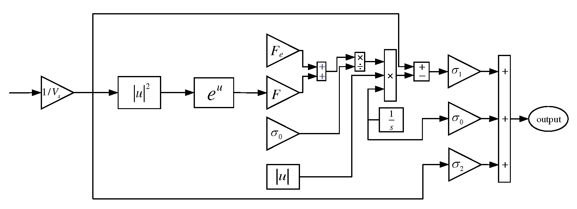
Figure 7.
Feedforward controller
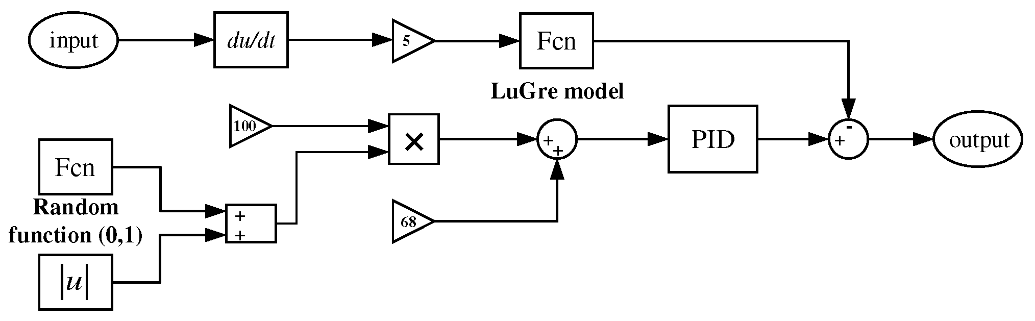
Figure 8.
Simulated comparison of friction compensation.

Figure 9.
B-spline Complex path.
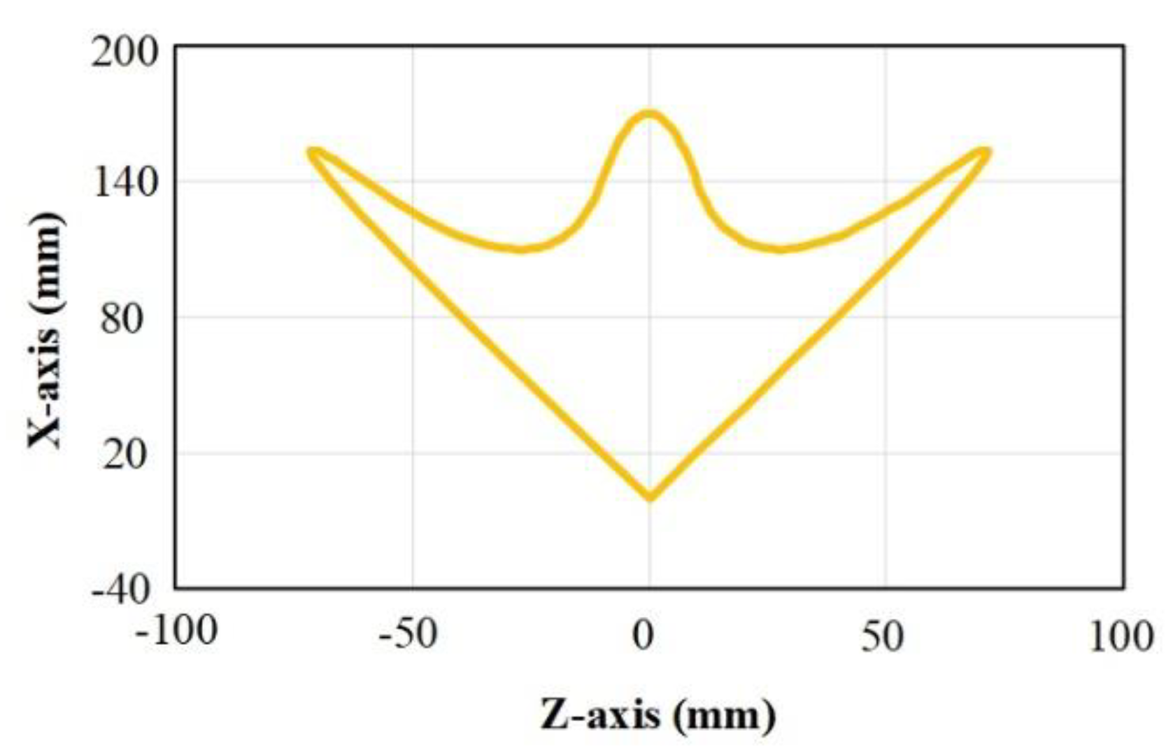
Figure 10.
Compensation result of feedrate error.

Disclaimer/Publisher’s Note: The statements, opinions and data contained in all publications are solely those of the individual author(s) and contributor(s) and not of MDPI and/or the editor(s). MDPI and/or the editor(s) disclaim responsibility for any injury to people or property resulting from any ideas, methods, instructions or products referred to in the content. |
© 2023 by the authors. Licensee MDPI, Basel, Switzerland. This article is an open access article distributed under the terms and conditions of the Creative Commons Attribution (CC BY) license (http://creativecommons.org/licenses/by/4.0/).
Copyright: This open access article is published under a Creative Commons CC BY 4.0 license, which permit the free download, distribution, and reuse, provided that the author and preprint are cited in any reuse.


