A Renormalizable Model of Quantum Gravity

John Ashmead

doi:10.20944/preprints202312.0850.v1

Preprint

Article

A Renormalizable Model of Quantum Gravity

This version is not peer-reviewed.

John Ashmead^*

This version is not peer-reviewed.

Downloads

374

Views

130

Comments

Submitted:

10 December 2023

Posted:

12 December 2023

Read the latest preprint version here

Abstract

Two main problems stand in the way of unifying quantum mechanics and general relativity. First, the treatment of time and space in quantum electrodynamics (QED) is not fully covariant. Second, the ultraviolet divergences in quantum general relativity are not easily renormalizable past the one loop level.In previous work, we ad- dressed the rst problem by promoting time from parameter to operator: with this the treatment of time and space in QED became fully covari- ant. The most obvious prediction was additional dispersion in time at the attosecond scale; such eects are falsiable with current technology. As an unexpected but welcome side-eect, this regularized the ultraviolet divergences in QED. We therefore ask \will promoting time to opera- tor regularize the ultraviolet divergences in quantum general relativity (QGR)?" Using the existing literature on QGR as a base, we show we can rewrite QGR with time as an operator. And that the ultraviolet diver- gences are contained in QGR just as they are in QED. We show that there are feasible tests which can distinguish between standard QGR and TGR. We conclude that TGR represents a renormalizable model of quantum gravity which is consistent with existing observational and experimental evidence and which is falsiable in principle.

Keywords:

quantum gravity

;

time

;

quantum mechanics

;

quantum electrodynamics

Subject:

Physical Sciences - Theoretical Physics

1. Introduction

Quantum mechanics (QM) and general relativity (GR) have modified our understanding of the physical world in depth. But they have left us with a general picture of the physical world which is unclear, incomplete, and fragmented. Combining what we have learned about our world from the two theories and finding a new synthesis is a major challenge, perhaps the major challenge, in today’s fundamental physics. – Carlo Rovelli [132]

Problem of Quantum Gravity

In quantum mechanics (QM) and general relativity (GR) we have two brilliantly confirmed theories that appear to be almost perpendicular to each other. Since they have very different domains of applicability it has not so far been possible to force a resolution. But the last few years have seen extraordinary progress in gravitational wave detection and multi-messenger astronomy [1,35,100,124] as well as equally extraordinary recent progress on the experimental side [10,18,20,27,31,80,82,87,124]. We should therefore be getting closer to finding a resolution.

There are two main problems making a resolution difficult:

The treatment of time and space in QM is not fully covariant.
There is currently no way to systematically renormalize higher order loops in quantum general relativity (QGR).

Promoting Time from Parameter to Operator

With respect to the first problem: in recent work [7,8,9] we asked “what breaks” if we force the issue by promoting time to an operator in quantum mechanics (QM) and quantum electrodynamics (QED). We used the Feynman path integral approach (FPI). We extended the paths from three dimensional – right/left; forward/back; upwards/downwards – to four dimensional, allowing the paths to move to future/past as well. From a human point of view this might be a trifle disorienting, but the math does not care about that. The rest of the FPI machinery was kept almost unchanged.

The approach (TQM for Time + QM) reduces to standard quantum mechanics (SQM) in the appropriate limits. But at short times there are differences that should be detectable with current technology. So TQM is falsifiable as well.

With respect to the second problem: we were concerned that with an additional dimension to integrate over, the familiar loop divergences would go from renormalizable to un-renormalizable. In fact the opposite happened; the combination of dispersion in time and entanglement in time made the loops self-regulating.

Quantizing Gravity

An obvious follow-on questions is “can we apply this approach to General Relativity”? We argue we can: if we quantize general relativity (GR) at the metric level and employ the de Donder or transverse-traceless gauge, the same methods that apply to QED apply to GR. The non-linear character of GR does not keep us from doing this. We refer to the result as TGR (Time + General Relativity).

Experimental Tests

Tests of TQM are feasible with current technology. The predictions are well-defined, so we expect that it will be confirmed/falsified in the near future. For purposes of this analysis we will assume that it will be confirmed.

Tests of TGR are harder. The best single test of TQM is the Heisenberg Uncertainty Principle in time. A comparable test in quantum general relativity might involve the use of planets moving at relativistic speeds with respect to each other. This is probably outside the scope of most laboratory budgets.

With that said, the number of proposed and arguably feasible tests of QGR is rapidly increasing. It is probably only a matter of time before QGR is confirmed/falsified. Again, we will assume that for purposes of this analysis it will be confirmed.

Ensembles of Gravitons

We have not found a direct test of TGR that seems suitable, but we have found a class of indirect tests that might work. In QGR it is natural to assume that the metric is really an average over an ensemble of gravitons, a variation on the emergent gravity idea (first proposed by Sakharov [135], subsequently brought to considerable prominence by Verlinde [160,161,162] and others). If we grant this assumption, then the predicted thermodynamic properties of the ensemble are very different in TGR. And it should be possible to probe them with decoherence experiments and other methods. We argue that TGR is therefore falsifiable in principle.

Outline of Paper

In his Quantum Field Theory in a Nutshell [172] Zee made quantum field theory (QFT) much more accessible by breaking the subject out into baby, child, and adult problems. We do the same thing here. We start with the non-relativistic case (baby problem), showing how to integrate four dimensional paths into the usual FPI formalism. Then we extend this to QED (child problem) letting the fields vary in all four dimensions. Then we move to quantum general relativity (the adult problem), including four dimensional paths in the analysis of graviton/matter and graviton/graviton interactions. We then verify that TGR does not have the ultraviolet (UV) divergences, before going on to experimental and observational tests of TGR. We also look at implications for dark energy ([16,21,22,34,45,88,98,104,127,142,158,166,167,168,177,178]) and dark matter ([4,6,15,33,46,86,89,97]). We conclude by arguing that while confirmation/falsification of TGR is a non-trivial problem, the odds of confirmation are reasonable and even falsification would have value from a scientific point of view.

2. Time as an Observable in Quantum Mechanics

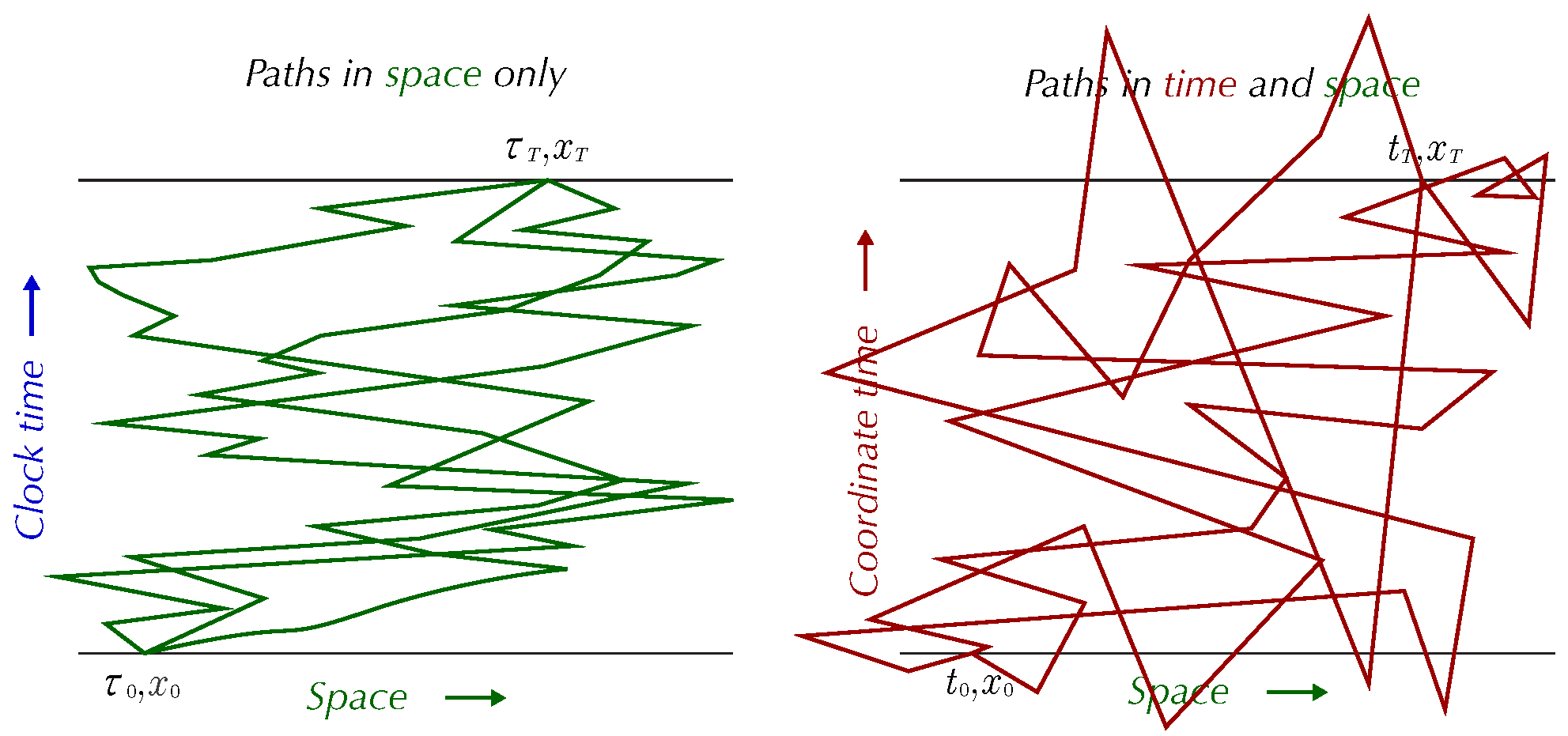
Figure 1. Paths in space; paths in time and space.

The work here has its starting point in the Feynman path integral approach (FPI) as originated by Stueckelberg and Feynman [52,53,54,55,148,149] and as further developed in [56,58,68,81,90,93,105,129,138,153,179,93,105].

Our initial goal is to promote time from parameter to operator. We chose FPI as the primary approach because with FPI the only change we had to make was to generalize the set of paths to extend in time just as they already did in space. The rest of the machinery we were able to leave largely alone.

We look at the non-relativistic (NR) and then the QED cases. Most of the key ideas show up in the NR case. To extend TQM to QED we have to shift from point particles to Fock space and to include both relativistic energies and the ability to create and annihilate particles.

Our two guiding principles are:

Complete covariance between time and space.
Consistency with the SQM results in the appropriate limit (usually time goes to infinity).

The great advantage of these two principles is that they leave us with no free parameters. And therefore ensure falsifiability.

2.1. Non-Relativistic Quantum Mechanics

As noted, the key idea is to promote the paths from 3D to 4D. A number of supporting ideas are required.

2.1.1. Clock Time

The first of these is clock time. For the moment, we define this as “what the lab clock measures”. This is also referred to as laboratory time, as in Busch [23]. This investigation is indebted not only to Busch but to many general reviews of the role of time in quantum mechanics: [24,40,47,102,103,119,139,176].

The clock time plays an essential role here; we reserve the symbol

τ

for it.

We do not mean the proper time. This would be different for each particle, so would make the analysis of the multiple particle case very difficult.

We will think of

τ

as the time of a nominal observer.

2.1.2. Coordinate Time

The paths extend into the future and into the past. They need a time coordinate along which to extend themselves. We therefore define coordinate time t as this time coordinate. Coordinate time is defined by the properties of

\vec{x}

plus covariance. We will shortly find it convenient to identify coordinate time as the time coordinate in the block universe picture.

2.1.3. Lagrangian and Action Unchanged

For both NR and QED cases we are able to reuse the existing Lagrangian. In the NR case we use a Lagrangian from Goldstein: [61]:

L [x_{τ}, {\dot{x}}_{τ}] = - \frac{1}{2} m {\dot{x}}^{μ} {\dot{x}}_{μ} - q {\dot{x}}^{μ} A_{μ} (x) - \frac{m}{2}

(2.1)

This gives the action:

S = \int_{0}^{T} d τ L

(2.2)

The path integral itself is defined as the sum over all paths weighed by the exponential of the action. To make this easier to visualize we slice time up into N slices, going from time equal zero to time T. Each slice covers an infinitesimal time

ε \equiv \frac{T}{N}

. Normally a path is defined as a series of points in three space,

π_{τ} \equiv ({\vec{x}}_{0}, {\vec{x}}_{1}, \dots, {\vec{x}}_{N})

. Here we define the paths in four space:

π_{τ} \equiv (x_{0}, x_{1}, \dots, x_{N})

. The kernel is defined as the sum over all such paths, weighted by the exponential of the action, with an overall normalization factor

C_{N}

K_{B A} = lim_{N \to \infty} C_{N} \int \prod_{n = 1}^{N - 1} d t_{n} d {\vec{x}}_{n} e^{ı ε \sum_{j = 1}^{N} L_{j}}

(2.3)

At the end of the calculation we let N go to infinity and thereby get the path integral – now understood as the appropriate QM kernel.

2.1.4. Convergence of Path Integrals

For all of this to make sense the individual integrals must converge. Normally this is insured by adding a small positive factor to the mass or the time. In QED, Wick rotation (replacing

τ \to - ı τ

) is perhaps most popular way to do this [90,179]. Neither approach works for us; there is no way to do either without violating covariance.

What we found was that neither approach is necessary. If we start with a normalizable wave function (i.e. not a

δ

function or a plane wave!) and do the integral from start to finish, each integration keeps the next one convergent. We showed this by using Morlet wave analysis to break any normalizable wave function up into a sum over Gaussians, showed it for any Gaussian, and then did the inverse sum.

While this might seem like a minor technical point – certainty it did to us at the time – it turned out to be key to showing that loops in TQM converge. If the initial wave function has a finite dispersion in time, that finite dispersion acts like a built-in regularizing factor. The integration over each slice keeps the next integral honest – or at least finite.

Note that the rate of convergence depends on the specifics of the initial wave function. Further we are not allowed to solve for a kernel directly; we must always solve for a kernel as applied to a specific wave function.

2.1.5. Schrödinger Equation

Usually we derive the FPI expression from the Schrödinger equation. But here we work in reverse, we go from the kernel to the Schrödinger equation:

\frac{\partial K}{\partial τ} = {lim}_{ε \to 0} \frac{K_{τ + ε} - K_{τ}}{ε}

(2.4)

which gives us:

- 2 m ı \frac{\partial ψ_{τ}}{\partial τ} = ((p_{μ} - q A_{μ}) (p^{μ} - q A^{μ}) - m^{2}) ψ_{τ}

(2.5)

We recognize this as the Feynman-Stückelberg equation (FS/T) from the Relativistic Dynamics (RD) program. In fact, this investigation is much indebted to the RD program. See for instance Horwitz, Fanchi, Piron, Land, Collins, and others [48,49,50,51,73,74,79,94].

The only difference is that in the RD program

τ

is a free parameter; here it is specifically defined as the clock time.

2.1.6. Free Solutions

The free solutions have the form:

ψ_{τ} (t, \vec{x}) = \frac{1}{4 π^{2}} exp (- ı E t + ı \vec{p} \cdot \vec{x} - ı ϖ τ)

(2.6)

with

ϖ_{p}

the clock energy defined by:

ϖ_{p} \equiv - \frac{E^{2} - {\vec{p}}^{2} - m^{2}}{2 m}

(2.7)

We will get the equivalent free solutions in QED by promoting

m \to E

and then including a spinor or a polarization factor for fermions and photons respectively.

2.1.7. Estimate of Initial Wave Function

Since we must always solve for a specific wave function we have to have a way to estimate them in particular cases. In the previous papers we got a crude but reasonable estimate by assuming we have an initial 3D wave function with known uncertainty in three momentum, then getting a maximum entropy estimate of the 4D wave function by using Lagrange multipliers.

〈{(Δ E)}^{2}〉 \sim 〈{(Δ p_{x})}^{2} + {(Δ p_{y})}^{2} + {(Δ p_{z})}^{2}〉

(2.8)

If we have the uncertainty in energy then we can estimate the initial wave function in energy as:

φ_{0} (E) = \sqrt[4]{\frac{1}{π σ_{E}^{2}}} e^{ı (E - \bar{E}) τ_{0} - \frac{{(E - \bar{E})}^{2}}{2 σ_{E}^{2}}}

(2.9)

σ_{E}^{2} = 2 {(Δ E)}^{2} = 2 (〈E^{2}〉 - {\bar{E}}^{2})

(2.10)

With the wave function in time as the Fourier transform:

φ_{0} (t) \equiv \sqrt[4]{\frac{1}{π σ_{t}^{2}}} e^{- ı \bar{E} t - \frac{{(t - τ_{0})}^{2}}{2 σ_{t}^{2}}}, σ_{t} = \frac{1}{σ_{E}}

(2.11)

2.1.8. Time Scales

There are two different time scales at work here. The time scales for t come from atomic units. They correspond to energies of order electron volts, therefore of order attoseconds and less.

But the time scale for the clock time

ϖ_{p}

is a million times slower than that. Taking bound state wave functions as a basis, the clock frequency is of order millionths of an electron volt and associated time scale of order picoseconds.

This provides a quick if partial explanation of the much debated transition from the quantum to the classic realm. At atomic times the clock time does not play a role,

ı \frac{\partial}{\partial τ} \approx 0

, the FS/T equation looks like the Klein-Gordon (KG) equation, and the wave function varies as rapidly in time as in space.

But consider the long (to an atomic particle) trip from interaction zone to detector. Now the effects of on-shell bits of the wave function (

ϖ_{p} \approx 0

) will tend to reinforce, off-shell bits to cancel, and the wave function that arrives at the detector will look as if it has magically gone on-shell. See for instance Tannor [154] on this sort of effect.

2.1.9. Definition of Clock Time in Terms of Quantum Time

The division of time into clock time and coordinate time was essential to the development of TQM in the previous papers. It is very difficult for a single time to successfully track both the quantum and classical aspects of time. At the same time (as it were), having two distinct time variables violates the principle of economy of ideas.

We therefore re-define the clock time as the expectation of the time operator over the wave function of the laboratory:

τ \equiv 〈ψ_{L a b} |t| ψ_{L a b}〉

(2.12)

We have shifted the weight of the analysis from the clock time, where we started, to the coordinate time. The clock time is now a mere convenience variable, useful but ultimately disposable.

And to further economize on ideas, we now redefine the coordinate time as the time part of the block universe picture. The paths are to be seen as objects that exist entirely in the block universe picture, with well-defined coordinate time endpoints, but no direct connection to the clock time. The clock time serves to divide up the paths in distinct sets and to make clear the connection of TQM to SQM, but no longer has a fundamental role to play.

2.1.10. Choice of Laboratory Frame

We had one failure to achieve full covariance; the specific choice of a laboratory frame picks out a preferred frame. We resolved this by noting that Weinberg [169] was able to define a pseudo-tensor corresponding to the energy-momentum of spacetime itself. This implies that we can choose the rest frame of local spacetime as the preferred frame. As this frame is an invariant, we have an invariant definition of the laboratory frame.

2.1.11. Falsification in Principle

We now have falsification in principle: we can solve the FS/T in a variety of cases, look for differences from the KG or the usual Schrödinger equation as the case requires, and thereby confirm or falsify TQM. However the actual effects are going to show at short times and high energies. In such cases we are looking not only at relativistic energies but also at particle creation and annihilation. To get to falsification in practice we need to extend this approach to QED.

2.2. Quantum Electrodynamics

Our primary target here is to summarize the recipe for turning an existing set of Feynman rules with time-as-parameter into the corresponding set of Feynman rules with time-as-observable. We worked these out in [9].

For the most part the derivations were straight-forward. Thinking of coordinate time (or coordinate energy) as a kind of fourth space dimension, albeit one that enters with opposite sign in some cases took care of most questions.

There are of course some subtleties. The principal ones are that:

We are primarily interested in short clock times, often short enough that the influence of the dependence on clock time can be neglected.
The elegance of the Feynman rules tends sometimes to obscure the physical meaning. In particular the use of contour integration at a key step makes the meaning of the virtual particles perhaps more opaque than is ideal. We discuss this further below.

2.2.1. Action

We were able to reuse the QED Lagrangians unchanged. But we had to define the action differently. The spin zero case is the simplest but still typical. In SQM we have the Lagrangian:

L^{S Q M} \equiv \frac{1}{2} (\partial_{τ} ϕ \partial^{τ} ϕ - \nabla ϕ \nabla ϕ - m^{2} ϕ^{2})

(2.13)

and the action is:

S^{S Q M} \equiv \int_{- \infty}^{\infty} d τ \int_{- \infty, - \infty, - \infty}^{\infty, \infty, \infty} d \vec{x} \frac{1}{2} (\partial_{τ} ϕ \partial^{τ} ϕ - \nabla ϕ \nabla ϕ - m^{2} ϕ^{2})

(2.14)

The Lagrangian in TQM is formally identical except that the clock time has been replaced by the coordinate time:

L^{T Q M} \equiv \frac{1}{2} (\partial_{t} ϕ \partial^{t} ϕ - \nabla ϕ \nabla ϕ - m^{2} ϕ^{2})

(2.15)

No surprise there.

But the action is now subtly different:

S_{T}^{T Q M} \equiv \int_{0}^{T} d τ \int_{- \infty, - \infty, - \infty, - \infty}^{\infty, \infty, \infty, \infty} d t d \vec{x} \frac{1}{2} (\partial_{t} ϕ \partial^{t} ϕ - \nabla ϕ \nabla ϕ - m^{2} ϕ^{2})

(2.16)

We have integrals for both coordinate time and clock time. The Lagrangian does not depend at all on the clock time, so that the canonical momenta either do not exist or are trivial, whichever term you prefer. Further, the integral over clock time is finite. We do not need to take the limit as clock time goes to plus and minus infinity, in fact we are usually far more interested in short clock times than long.

In either case, every vertex in momentum space will have an accompanying:

δ^{4} (\sum_{o u t} p_{o u t} - \sum_{i n} p_{i n})

(2.17)

in the coordinate energy and momenta. But it will only get a:

δ (\sum_{o u t} ϖ_{o u t} - \sum_{i n} ϖ_{i n})

(2.18)

in clock time if we take

τ \to \pm \infty

. (We have E the complementary operator of the coordinate time t;

ϖ

the complementary variable of the clock time

τ

.) If we are not taking the

τ \to \pm \infty

limit we will have to compute the integral over clock time by hand, using the appropriate factors of

exp (- ı ϖ_{p} τ)

2.2.2. Feynman-Stückelberg Equations

As a practical matter we found that starting with the FS/T equations provided a more robust extrapolation of the NR to the QED case than starting with the action. The actions are useful as a summary of the properties, but the FS/T equations are definitive. Details are in the previously cited works.

For spin zero we replace

m \to w

ı \frac{\partial}{\partial τ} ψ = - \frac{w^{2} - {\vec{k}}^{2} - m^{2}}{2 w} ψ

(2.19)

For photons we assume we are in Lorentz gauge, so that each component obeys its own KG equation:

- 2 w ı \frac{\partial}{\partial τ} A^{ν} = (w^{2} - {\vec{k}}^{2}) A^{ν}

(2.20)

And for fermions we again take advantage of the fact that with a bit of manipulation the Dirac equation can also apply to each component separately:

- ı γ_{0} \frac{\partial}{\partial τ} ψ_{τ} = (/ p - m) ψ_{τ}

(2.21)

With these choices the propagators can be written as a polarization or spin factor times the spin zero propagator. (This is also true in the QED case, see [92]).

2.2.3. Free Wave Functions

With the FS/T equations we have their corresponding free solutions almost by inspection. We focus, as usual, on the spin zero case.

Explicit Free Wave Functions

SQM free wave function:

ϕ_{k} (x) = \frac{1}{\sqrt{V}} \frac{1}{\sqrt{|2 ω_{\vec{k}}|}} exp (- ı ω_{\vec{k}} τ + ı \vec{k} \cdot \vec{x}), ω_{\vec{k}} \equiv \sqrt{{\vec{k}}^{2} + m^{2}}

(2.22)

TQM free wave function:

ϕ_{k} (x) = \frac{1}{\sqrt{TV}} \frac{1}{\sqrt{|2 w|}} exp (- ı ϖ_{k} τ - ı k x), ϖ_{k} \equiv - ı \frac{w^{2} - {\vec{k}}^{2} + m^{2}}{2 w}

(2.23)

The changes are:

Box normalization goes to hyper box normalization: $V \to TV$ . We assume periodic boundary conditions.
Three vectors go to four vectors: $\vec{k} \cdot \vec{x} \to k x$ .
Energy normalization goes from on-shell energy to free energy: $w_{\vec{k}} \to w$ .
Dependence on clock time given by clock frequency.

The first two changes are direct results of rule one.

The use of box normalization is a great help with dimension checking. Once the dimension checking is done, it is often simpler to work with continuous normalization. In this case the factors

{(2 π)}^{3}

go to

{(2 π)}^{4}

The presence of a box in time – the factor of

T

– may be a bit unnerving at first. In QED we can think of this as a box in time large enough to contain the entire interaction of interest. In GR, this time range may be up to 13.8 billion years, so as boxes go, this is a large one. In this case, we may prefer a more sophisticated treatment using a manifold of hyper-boxes, keeping the individual boxes at a more reasonable size.

The shift from the on-shell energy to the unconstrained energy is an aspect of the shift from time as parameter (constrained) to time as observable (unconstrained). This same rule is applied to the Dirac spinors: all occurrences in them of the on-shell/contrained

E_{\vec{p}}

are replace by the unconstrained E.

As to the fourth point, in TQM almost all the dependence on time is through the dependence on coordinate time. For the sort of high-speed interactions we are primarily interested in, the clock time is likely to be essentially frozen, only coming into play on the legs.

It is often helpful to write the coordinate time as:

t \equiv τ + δ t

(2.24)

the coordinate energy as:

w \equiv w_{\vec{k}} + δ w

(2.25)

with the usually reasonable expectation that both

δ t

and

δ w

will be small in practice.

Fock Space

This lets us define the Fock space in terms of sums of the appropriately symmetrized free wave functions. It is given in the occupation representation by:

|\{n_{k}\}〉

(2.26)

where n is an integer from zero to infinity and the wave functions are fully symmetric.

The creation and annihilation operators are defined by their effects in Fock space:

a_{k} |n_{k}〉 = \sqrt{n_{k}} |n_{k} - 1〉, a_{k}^{†} |n_{k}〉 = \sqrt{n_{k} + 1} |n_{k} + 1〉

(2.27)

with 4D commutators:

[a_{k}, a_{k^{'}}^{†}] = δ^{4} (k - k^{'})

(2.28)

All other commutators are zero. We make no use of the common interpretation in terms of harmonic oscillators.

In and Out Wave Functions

These are given by sums over the free wave functions above.

Feynman Propagators

SQM The propagator is defined in terms of time ordered products of the free wave functions:

ı Δ_{τ_{x} τ_{y}}^{S} (\vec{x} - \vec{y}) \equiv 〈0 |T \{ϕ_{τ_{x}}^{S} (\vec{x}), ϕ_{τ_{y}}^{S} (\vec{y})\}| 0〉

(2.29)

We pause the derivation at what is normally treated as an intermediate step:

ı S_{τ} (k) = \frac{ı}{{(2 π)}^{3}} (\frac{e^{- ı ω_{\vec{k}} τ}}{2 ω_{\vec{k}}} θ (τ) + \frac{e^{- ı ω_{\vec{k}} τ}}{2 ω_{\vec{k}}} θ (- τ))

(2.30)

These are Feynman boundary conditions; as noted, good for S matrix calculations, but problematic for loop calculations in TQM. We will refer to this as the “unpacked” form.

The next step in the derivation is to replace the positive time branch with a contour integral:

\frac{e^{- ı ω_{\vec{k}} τ}}{2 ω_{\vec{k}}} θ (τ) = \frac{ı}{2 π} \int_{- \infty}^{\infty} d ω \frac{e^{- ı ω τ}}{(ω - ω_{\vec{k}} + ı ε) (ω + ω_{\vec{k}})}

(2.31)

and the negative time with a similar contour integral. Combined, they give us the familiar expression for the propagator:

ı Δ_{ω}^{S} (\vec{k}) = \frac{ı}{ω^{2} - {\vec{k}}^{2} - m^{2} + ı ε}

(2.32)

This looks four dimensional; that’s not quite correct. The integral over energy is a contour integral. The value of the energy is effectively fixed by the value at the residue forcing the energy – appearances not withstanding – back on shell. This elegant trick makes the integrals easier to do but somewhat deceptive in appearance. TQM will replace this contour integral with a real one.

TQM TQM can be handled the same way, but with four dimensions in play rather than three. Again start with the definition of the propagator:

ı Δ_{x y} (x - y) = 〈0 |T \{ϕ_{x} (x), ϕ_{y} (y)\}| 0〉

(2.33)

We again use Feynman boundary conditions, to keep the development in parallel with SQM. But we stop the derivation just before the trick with the contour integral:

ı Δ_{x y} (x - y) = \frac{1}{{(2 π)}^{4}} \int d^{4} k \frac{e^{- ı ϖ_{k} τ_{x y} - ı k (x - y)}}{2 w} θ (τ) - \frac{e^{- ı ϖ_{k} τ_{x y} - ı k (x - y)}}{2 w} θ (- τ)

Note that the second term in TQM differs from the second term in SQM by the overall sign and by the sign of the clock frequency term. We are already integrating over w. We can see that the w integral is real; that off-shell values will contribute to the result. Effectively we have moved from virtual fluctuations in energy to real ones. This is what changing time from parameter to observable means in the context of propagators.

The value of w does depend on the choice of frame; see earlier comments about the use of the rest frame of spacetime to eliminate this choice.

With the same approach we have the propagator for photons in Lorentz gauge:

ı D_{τ}^{μ ν} (x) = - \frac{ı g^{μ ν}}{{(2 π)}^{4}} \int \frac{d w d \vec{k}}{2 w} (exp (- ı ϖ_{k} τ - ı k x) θ (τ) - exp (- ı ϖ_{k} τ + ı k x) θ (- τ))

(2.34)

and the propagator for fermions:

ı S_{τ} (p) = \frac{ı}{{(2 π)}^{4}} \int d^{4} p \frac{/ p + m}{2 E} (e^{- ı ϖ_{p} τ_{x y} - ı p (x - y)} θ (τ) - e^{- ı ϖ_{p} τ_{x y} - ı p (x - y)} θ (- τ))

The derivation of the photon and fermion propagators depended on the ability to find a gauge in which each component separately obeyed the KG equation. We then mapped the SQM KG equation to the TQM KG equation:

K^{S Q M} = \frac{ı}{k^{2} + ı ε} \Rightarrow K^{T Q M} = \frac{exp (- ı ϖ_{k} τ)}{2 w} θ (τ) - \frac{exp (- ı ϖ_{k} τ)}{2 w} θ (- τ)

(2.35)

We have not as yet extended TQM to Yang-Mills theories. Given that our experience was that almost all of the difficulties happened in the promotion from NR to spin zero we expect technical difficulties but not conceptual ones in that extension.

2.2.4. Vertexes

In QED there is only the one vertex term:

- e {\bar{ψ γ}}_{ν} A^{ν} ψ

(2.36)

As discussed earlier, in TQM each vertex will get a delta function in the coordinate momenta. If we are taking the limit as

τ \to \pm \infty

we will also get a

δ

function in clock energies. But for shorter times, we will generally want to go to the unpacked forms (of both SQM and TQM) and work out the dependence on clock time explicitly.

2.2.5. Measurable Differences between SQM and TQM

The driving difference between SQM and TQM is the promotion of time from parameter to operator. This implies the paths go from 3D to 4D, the wave functions have dispersion in time as well as in space, and so forth. There are technical questions as to normalization and boundary conditions but they are secondary.

If we want to see differences between SQM and TQM we will generally have to look at short times; attoseconds or smaller. Fortunately our reach into the attosecond realm is rapidly increasing. The recent award of the Nobel prize for such work [107] is a strong sign of this.

Currently the shortest attosecond scale pulses are now down to about 53as [91] which is still too large. But with skillful experimental design we can push well below that. For instance Ossiander et al [116] were able to probe down to sub-attosecond levels.

The scope of the expected effects is great: any time-dependent phenomena will show some effect.

Tests of the Heisenberg uncertainty principle (HUP) in time/energy are the most promising. If the HUP applies in energy/time as it does in space/momentum, then when a wave packet passes through a small gate in time (think very rapid camera shutter) it will be diffracted: the resulting uncertainty in time at a detector will be arbitrarily great. But if the HUP does not, then the wave packet will be clipped: the resulting uncertainty in time at a detector will be arbitrarily small. (In practice the small gate could be replaced by a probe wave packet engineered to have a small dispersion in time.) The experiment is a knife: the effect is either arbitrarily large or arbitrarily small.

3. Quantizing the Metric

3.1. Metric as Quantum Field

There is an extraordinary literature on GR; we have found the following particularly helpful: [2,29,70,101,134,140,151,155,157,163,173].

Our goal is now to apply the approach used for QED to QGR. To do this we will treat the metric as a field, no different in principle from any other field, and slot it into the machinery developed for QED.

This should then address both of the problems that inspired this work:

The treatment of time will be fully consistent with that of space. As we saw, this is not entirely true of QED; it is certainly a fundamental requirement for any quantization of GR.
The perturbative expansion of the action in Feynman diagrams is not convergent: the loop diagrams do not converge. The first order loop diagrams can be renormalized but the number of renormalization constants increases without limit as the number of loops increases.

Before settling on the metric as the target we consider alternatives. The principal alternative is to quantize at the spacetime level. There are two problems with this:

Which spacetime? There are many: string theory, loop quantum gravity, causal set theory, causal dynamic triangulation, and so on.
Most show their effects at the Planck scale. For the most part, this means there is no real prospect of falsifying any results.

By working at the metric level we are working with a kind of lowest common denominator of most or all of the proposed spacetimes. If we can quantize at the metric level, then experimental or observational discrepancies can direct our attention to effects of some underlying spacetime.

We have found it helpful to think in terms of the Mercator projection maps of the world found in schoolrooms everywhere. The Mercator projection stretches the distances at the poles so you can not just apply ruler to map to get a correct distance. It is easy enough to develop a metric that corrects for this.

But consider now a traveler using a Mercator map to get from one place to another. The metric will give the true distance from a flying crow’s point of view. But if the traveler has to climb mountains or descend into oceans to follow the straight course from A to B, the travel time metric will give wildly different results from the Mercator metric.

For us, then spacetime plays the role of the underlying geography. We focus on the metric because with that we can get falsifiable results, but we are always mindful of the possibility that there may be more to the question than just the metric.

We take the metric as target and assume that there are also quantized disturbances in the metric (ripples on the map). We follow the literature in referring to these as gravitons. They may be quasi-particles or fundamental representations of an irreducible Lorentz group: we are not fussy. So long as we can quantize them in a consistent way and predict experimental or observational results, we have what we need.

We can write the metric as:

g_{μ ν} \to η_{μ ν} + h_{μ ν}

(3.1)

where

η

is the Minkowski metric (using particle conventions):

η = (\begin{matrix} + 1 & 0 & 0 & 0 \\ 0 & - 1 & 0 & 0 \\ 0 & 0 & - 1 & 0 \\ 0 & 0 & 0 & - 1 \end{matrix})

(3.2)

Much of the literature uses a variable dimension

D \geq 4

. We will content ourselves with the usual four dimensions here.

We can break up the h into classical and quantum parts:

g_{μ ν} = η_{μ ν} + {\bar{h}}_{μ ν}^{(c l a s s i c a l)} + {\hat{h}}_{μ ν}^{(q u a n t u m)}

(3.3)

Often it will be useful to perform a coordinate transformation to flatten out the classical part of h, leaving us with just the Minkowski metric and the quantum fluctuations on it:

g_{μ ν} \to η_{μ ν} + {\hat{h}}_{μ ν}

(3.4)

3.2. Free Gravitons

We now build up the free wave functions and propagator for gravitons. The treatment here is abbreviated from [68,84,157,159].

The matter free action in general relativity is:

\int d τ d \vec{x} \sqrt{- g} R

(3.5)

If we vary the action with respect to the metric we get the free Einstein equations of motion. If we take a second variation, we get the propagator. For instance [159]:

K_{μ ν, α β} = \frac{δ_{μ α} δ_{ν β} + δ_{μ β} δ_{ν α} - δ_{μ ν} δ_{α β}}{k^{2} + ı ε}

(3.6)

This is more complex than we would like.

We can simplify the propagator by making an appropriate gauge choice. We want one where each element of the metric obeys the KG equation by itself; then we can apply equation 2.35 to get the TQM propagator.

The metric starts as a symmetric four-by-four matrix, with ten degrees of freedom. The metric must satisfy the four Bianchi identities; this leaves have only six degrees of freedom. We can use our freedom to choose the four coordinates to reduce the number of degrees of freedom by four, leaving us with only two degrees of freedom.

We take advantage of this to impose the de Donder (or transverse traceless) gauge condition:

\partial^{μ} h_{μ ν} - \frac{1}{2} \partial_{ν} h_{μ}^{μ} = 0

(3.7)

We can simplify still further by defining:

{\bar{h}}_{μ ν} \equiv h_{μ ν} - \frac{1}{2} h η_{μ ν}

(3.8)

This gives the simple form for the matter-free Einstein equation:

{\bar{h}}_{μ ν} = 0

(3.9)

We can get the familiar h back from

\bar{h}

by:

h_{μ ν} \equiv {\bar{h}}_{μ ν} - \frac{1}{2} \bar{h} η_{μ ν}

(3.10)

With only two actual degrees of freedom we can describe a graviton using only two polarization matrices. For example assume the graviton is traveling in the z direction:

k_{μ} = (w_{\vec{k}}, 0, 0, w_{\vec{k}})

(3.11)

We can take the two polarization matrices as:

H_{μ ν}^{1} = (\begin{matrix} 0 & 0 & 0 & 0 \\ 0 & 1 & 0 & 0 \\ 0 & 0 & - 1 & 0 \\ 0 & 0 & 0 & 0 \end{matrix}), H_{μ ν}^{2} = (\begin{matrix} 0 & 0 & 0 & 0 \\ 0 & 0 & 1 & 0 \\ 0 & 1 & 0 & 0 \\ 0 & 0 & 0 & 0 \end{matrix})

(3.12)

These are sometimes called plus (+) and cross (x) polarizations.

We can write the graviton wave function in terms of these two polarizations:

G_{k}^{r} (τ, \vec{x}) = \frac{1}{\sqrt{2 V ω_{\vec{k}}}} H_{k}^{r} e^{- ı ω_{\vec{k}} τ + ı \vec{k} \cdot \vec{x}}

(3.13)

The corresponding TGR free wave function is:

G_{τ}^{r, k} (t, \vec{x}) = \frac{1}{\sqrt{2 T V w}} H_{k}^{r} e^{- ı ω_{\vec{k}} τ - ı w t + ı \vec{k} \cdot \vec{x}}

(3.14)

3.2.1. Fock Space in TGR

This gives us the Fock space as the sum over these free wave functions:

|\{n_{k}^{r}\}〉

(3.15)

With creation and annihilation operators:

{\hat{H}}_{k}^{r} |n_{k}^{r}〉 = \sqrt{n_{k}^{r}} |n_{k}^{r} - 1〉, {\hat{H}}_{k}^{r †} |n_{k}^{r}〉 = \sqrt{n_{k}^{r} + 1} |n_{k}^{r} + 1〉

(3.16)

Commutation relations:

[{\hat{H}}_{k}^{r}, {\hat{H}}_{k^{'}}^{r^{'} †}] = δ^{4} (k - k^{'}) δ_{r r'}

(3.17)

And wave function operators:

G_{τ}^{T} (t, \vec{x}) = \sum_{k} \sum_{r = 1, 2} \frac{1}{\sqrt{2 TV w}} ({\hat{H}}_{k}^{r} e^{- ı ω_{k} τ + ı k x} + {\hat{H}}_{k}^{† r} e^{ı ω_{k} τ - ı k x})

(3.18)

3.2.2. TGR Propagators

And same procedure as with TQM gives us the free graviton propagator. We start with the (clock) time-ordered product:

ı K (x - y) = 〈0 |T \{G (x), G (y)\}| 0〉

(3.19)

We use same approach as for TQM. The treatment is essential;y the same as for the photon. The result is:

K_{μ ν}^{α β} = I_{μ ν}^{α β} (\frac{exp (- ı ϖ_{k} τ)}{2 w} θ (τ) - \frac{exp (- ı ϖ_{k} τ)}{2 w} θ (- τ))

(3.20)

with side-definition:

I_{μ ν}^{α β} \equiv \frac{1}{2} (δ_{μ}^{α} δ_{ν}^{β} + δ_{μ}^{β} δ_{ν}^{α})

(3.21)

I ensures that the graviton matrix stays symmetric.

We therefore have the free TGR wave functions and propagator. Note that during the derivation we required that the individual components of the graviton obey the KG equation. But now we have established the mapping from SQM to TQM, we are permitted to undo the gauge transformations that achieved this simplicity. For instance, we could return to the article-title propagator and map it to its TQM equivalent:

K_{μ ν, α β} \to (δ_{μ α} δ_{ν β} + δ_{μ β} δ_{ν α} - δ_{μ ν} δ_{α β}) (\frac{exp (- ı ϖ_{k} τ)}{2 w} θ (τ) - \frac{exp (- ı ϖ_{k} τ)}{2 w} θ (- τ))

(3.22)

4. Action for Quantum General Relativity

“Wheeler’s often unconventional vision of nature was grounded in reality through the principle of radical conservatism, which he acquired from Niels Bohr: Be conservative by sticking to well-established physical principles, but probe them by exposing their most radical conclusions.” – K. S. Thorne [156]

We first note our obligation to workers in the area of Quantum Gravity as [25,28,36,37,38,39,41,42,43,44,59,68,83,115,123,133,147,152,169]

At this point we have what we need to build a renormalizable model of quantum gravity. We do this by applying the methods of TQM to the metric of QGR. We are largely taking a kind of “direct product” of the two approaches, although the non-linear character of gravity and the fact that general relativity expresses itself as geometry add complications.

We start by taking the “cosmic time” as the equivalent of laboratory time. Then we look at the expansion of the action in powers of the graviton. The propagator provides a convenient way to categorize this. We have pure matter, matter-graviton, and graviton-graviton terms. Once we have done this we will have enough to apply our Feynman rules recipe to promote QGR to TGR.

We will refer to QGR with time-as-parameter as standard QGR or SGR.

4.1. Cosmic Time As clock Time

To develop in parallel with TQM, we need a clock time to serve as reference. For the development here the specific choice of clock time is not critical; we only require a well-defined and consistent choice.

We may think of the universe as an unusually large laboratory clock. We therefore use as our laboratory time the cosmic time as defined in the

Λ - C D M

model.

And ultimately we can define the cosmic time, in its turn, as the expectation of the coordinate time variable of the wave function of the universe

U

τ \equiv 〈 U | t |U〉

(4.1)

From here to the end, references to

τ

will refer to cosmic time.

4.2. Expansion of the Action in Powers of the Quantum Operators

We have found Jakobsen [84] particularly helpful. He is approaching QGR from a QFT perspective, as we are, and gives a detailed account of the propagator, vertexes, and so on. As usual we will focus on the spin zero case to define the rules, then extend to include photons and fermions.

We start with the Einstein-Hilbert and matter actions. We work in parallel to the development in TQM. The QGR action is given by:

\int d τ d \vec{x}} \sqrt{- g} (\frac{2 R}{κ^{2}} + L_{M})

(4.2)

with

κ

defined as:

\begin{matrix} κ^{2} & \equiv & 32 π G_{N} \end{matrix}

(4.3)

This lets us mark the various terms in the Feynman diagrams by

κ

to reflect how many powers of

G_{N}

they correspond to.

We have immediately the corresponding action for TGR:

\int d τ {d x}^{4} \sqrt{- g} (\frac{2 R}{κ^{2}} + L_{M})

(4.4)

The two Lagrangians are formally the same, but all references within to clock time have been replaced with references to coordinate time. We will be interrogating this action with in powers of the graviton operator

\hat{h}

g \to g + \hat{h}

(4.5)

The measure for the path integral looks formally the same. But as earlier, each field is define over four dimensions rather than three. For instance at clock time

τ

we will be varying the metric over its values for the entire block universe (not merely one time-slice of the block universe):

D h_{μ ν} D ϕ

(4.6)

The Einstein equations are derived by varying the action with respect to the fields:

\frac{δ \sqrt{- g} (\frac{2 R}{κ^{2}} + L_{M})}{δ h_{μ ν}} + \frac{δ \sqrt{- g} (R + L_{M})}{δ ϕ} = 0

(4.7)

To help with power counting, we work with a scaled graviton field:

{\tilde{h}}_{μ ν} \equiv \frac{h_{μ ν}}{κ}

(4.8)

There are three cases we will look at:

Classical gravity; quantized matter. The matter waves are traveling over a classical sea of gravitons.
Quantum interactions between gravity and matter. We look at $h ϕ, h ϕ^{2}, h^{2} ϕ, h^{2} ϕ^{2}$ terms.
Gravity self-interactions. We will focus on the three graviton vertex, although in practice the four graviton vertex may also be significant.

4.3. Quantum Matter/Classical Gravity Interactions

We look first at classical gravity, quantum matter. Here we get classical gravity as merely the first term in an expansion of the action. Oppenheim has argued that gravity should be seen as ultimately classical [110,111,112,113,114] so that the treatment of gravity should stop here. In this context this is a minority but a necessary position.

There are a number of analyses of quantum matter moving in a curved space, including [74,75,76,77,78,164]. Any of those might serve as a starting point for the analysis here.

We focus on the matter action, taking the metric as a given. In SGR this is:

\int \sqrt{- g} d^{4} x L_{M}

(4.9)

with the normal derivatives being replaced by covariant derivatives:

\partial_{μ} \to D_{μ}

We promote this action to a TQM action by turning all internal

τ \to t

and adding an integral over clock time:.

\int \sqrt{- g} d^{4} x L_{M} \to \int d τ \int \sqrt{- g} d^{4} x L_{M}

(4.10)

We look first at the spin zero case. For spin zero the covariant derivative and the ordinary derivative are the same. Therefore in the spin zero case, at this order we replace the flat Minkowski metric with the curved but classical Einstein metric and (in TQM) include the integrals over 4D paths, but have no further changes to make:

S = \int d τ {d x}^{4} \sqrt{- g} \frac{1}{2} (\partial_{μ} ϕ \partial^{μ} ϕ - μ^{2} ϕ^{2})

(4.11)

For photons we have:

S = - \int d τ \int d^{4} x \sqrt{- g} F_{a b} F_{c d} g^{a b} g^{b d}

(4.12)

The covariant derivatives do not vanish but they do the next best thing, the Christoffel symbols cancel out.

F_{μ ν} \equiv D_{μ} A_{ν} - D_{ν} A_{μ} = \partial_{μ} A_{ν} - \partial_{ν} A_{μ}

(4.13)

Therefore the case for photons is the same as for spin zero particles: adjust to life on a curved metric and include paths in time as well as space. But again nothing particularly tricky.

For fermions we have our first taste of real complexity:

S = \int d τ \int d^{4} x \sqrt{- g} \bar{ψ} (ı D_{μ} - {e A}_{μ}) γ^{μ} ψ

(4.14)

The covariant derivative does not reduce to the normal partial derivatives:

{ı \partial}_{μ} γ^{μ} {\to ı \partial}_{μ} γ^{μ} + ı Γ_{μ ν}^{μ} γ^{ν}, Γ_{μ ν}^{μ} = \partial_{ν} (ln \sqrt{|g|})

(4.15)

We have:

S = \int d τ \int d^{4} x \sqrt{- g} \bar{ψ} ({ı \partial}_{μ} + {ı \partial}_{μ} (ln \sqrt{|g|}) - {e A}_{μ}) γ^{μ} ψ

(4.16)

We can if we wish treat the Christoffel term as an effective addition to the vector potential:

A_{μ} \to A_{μ} + \frac{1}{e} p_{μ} (ln \sqrt{|g|})

(4.17)

where we have rewritten the

ı \partial

as a momentum operator acting on the

ln \sqrt{|g|}

There are more sophisticated ways of modeling the behavior of fermions in curved space, see for instance [141]. Since our primary focus here is on the behavior of gravitons we leave this question unexplored.

4.4. Quantum Matter/Graviton Interactions

We now look at the quantum matter/graviton interactions. We are concerned with cases where we have one power of the graviton field and one or two powers of the matter fields in play.

4.4.1. Action

Again we start with the spin zero case, with action:

\int d τ \sqrt{- g} \frac{1}{2} (\partial_{μ} ϕ \partial^{μ} ϕ - μ^{2} ϕ ϕ)

(4.18)

Again we switch to a locally Minkowskian frame. We expand the metric with lowered indices to the first power of the graviton operator:

g_{μ ν} = η_{μ ν} + {\hat{h}}_{μ ν}

(4.19)

The graviton with raised indices is the inverse of that, so the graviton operator enters with opposite sign:

g^{μ ν} \approx η^{μ ν} - {\hat{h}}^{μ ν}

(4.20)

We must also include the density. To first order in the graviton operator we have:

\sqrt{- g} = 1 + \frac{1}{2} \hat{h}, \hat{h} \equiv {\hat{h}}_{μ}^{μ}

(4.21)

4.4.2. Hybrid Matter/Graviton Particles

We are faced with a slight twist here. Normally the propagator part of a Feynman diagram expansion represents two powers of the same species of particles. But here we have terms with powers of

h ϕ, h A, h ϕ

appearing. Appearing in the expansion at the propagator level suggests they may have an important role to play.

For now, we will treat them as hybrid particles. Think of them as normal particles strongly coupled to spacetime.

The most interesting case is graviton/photon hybrids. Both travel at the same speed, c, and we know that photons can be coaxed into forming hybrid particles with sound, i.e. phonon polaritons [72].

We will refer to these as “gotons” – gravitons + photons. Since the coupling of a graviton to anything depends on its energy, they are most likely to appear in cases where high energy gravitons are created next to high energy photons. If they succeed in hybridizing, we can see the graviton half as a ripple in spacetime that accompanies its companion photon, like a flying fish teaming up with a diving bird.

In the section on experimental and observational tests we will suggest several places where they might be looked for. The odds are not good, but if the long odds can be overcome, the scientific and practical possibilities may be significant.

4.4.3. Three Point Interactions

We turn now to more conventional interactions.

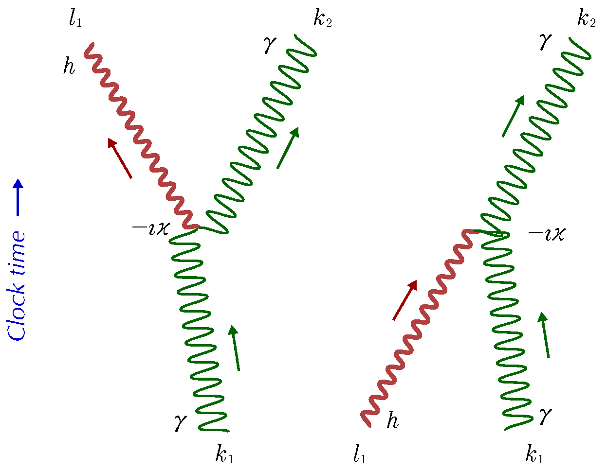
Figure 2. Graviton spin-zero scattering.

Spin Zero

The action to first order in h is:

S^{ϕ} (h) = - \frac{1}{2} \int d^{4} x h^{μ ν} ϕ_{, μ} ϕ_{, ν} + \frac{1}{4} \int d^{4} x h_{μ}^{μ} (ϕ^{, ν} ϕ_{, ν} - m^{2} ϕ^{2})

(4.22)

Per Jakobsen, the vertex is:

V^{(ϕ^{2} h) μ ν} (p, k, m) = I_{α β}^{μ ν} p^{α} k^{β} - \frac{p k - m^{2}}{2} η^{μ ν}

(4.23)

We normal order the operators at the vertex. The cases are:

$a^{†} h a$ – spin zero particle absorbs a graviton
$a^{†} h^{†} a$ – spin zero particle emits a graviton
$a^{†} a^{†} h$ – graviton emits a spin zero, anti spin zero pair
$h^{†} a a$ – spin zero, anti spin zero pair consume each other and give off a (rather high energy) graviton.

The first two represent quantum interactions of spin zero particles with a metric. The latter two represent variations on Hawking radiation.

The second and fourth represent ways that spin zero particles can pump energy into a metric (and vice versa).

Photons

We note that as before the covariant derivatives reduce to ordinary partial derivatives so in this respect this is similar to the spin zero case.

S^{{γ}} = \int d τ \int \sqrt{- g} d t d \vec{x} \frac{1}{4} F_{μ ν} F^{μ ν}

(4.24)

We have a coupling to the trace of the graviton, coming from the density:

V^{{γ}} = \frac{h_{α}^{α}}{8} (F_{μ ν} F^{μ ν})

(4.25)

And we have a more complicated coupling from the raised form of the metric:

(A_{μ, ν} - A_{ν, μ}) g^{μ α} g^{ν β} (A_{α, β} - A_{β, α})

(4.26)

which to first order gives:

(A_{μ, ν} - A_{ν, μ}) h^{μ α} η^{ν β} (A_{α, β} - A_{β, α}) + (A_{μ, ν} - A_{ν, μ}) η^{μ α} h^{ν β} (A_{α, β} - A_{β, α})

(4.27)

We have the same set of possible couplings as for the spin zero case.

Fermions

Again we start with the action:

S^{f} = \int d τ \int d t d \vec{x} \sqrt{- g} \bar{ψ} (ı D_{μ} - A_{μ}) γ^{μ} ψ

(4.28)

For the trace term, we drop the covariant derivative part:

V^{{e}} = \frac{h_{α}^{α}}{2} ({ı \partial}_{μ} γ^{μ} - {e A}_{μ} γ^{μ})

(4.29)

The metric replacement in the action acts once:

\bar{ψ} (h^{μ ν} ({ı \partial}_{μ} - {e A}_{μ}) γ_{ν}) ψ

(4.30)

And we have the same set of possible couplings as in the spin zero case.

4.4.4. Higher Order Corrections

There are order

h^{2}

and higher terms to consider, but for a first attack on the problem the first order should suffice.

The key point is that any quantum particle will experience a kind of quantum friction with the metric, even in flat space. This means there will be a constant interchange of energy and information between metric and particle.

While this may not be detectable at the single graviton level, if we model the metric as an ensemble of gravitons, there may be observational and experimental possibilities.

4.5. Graviton/Graviton Interactions

Figure 3. Three graviton vertex.

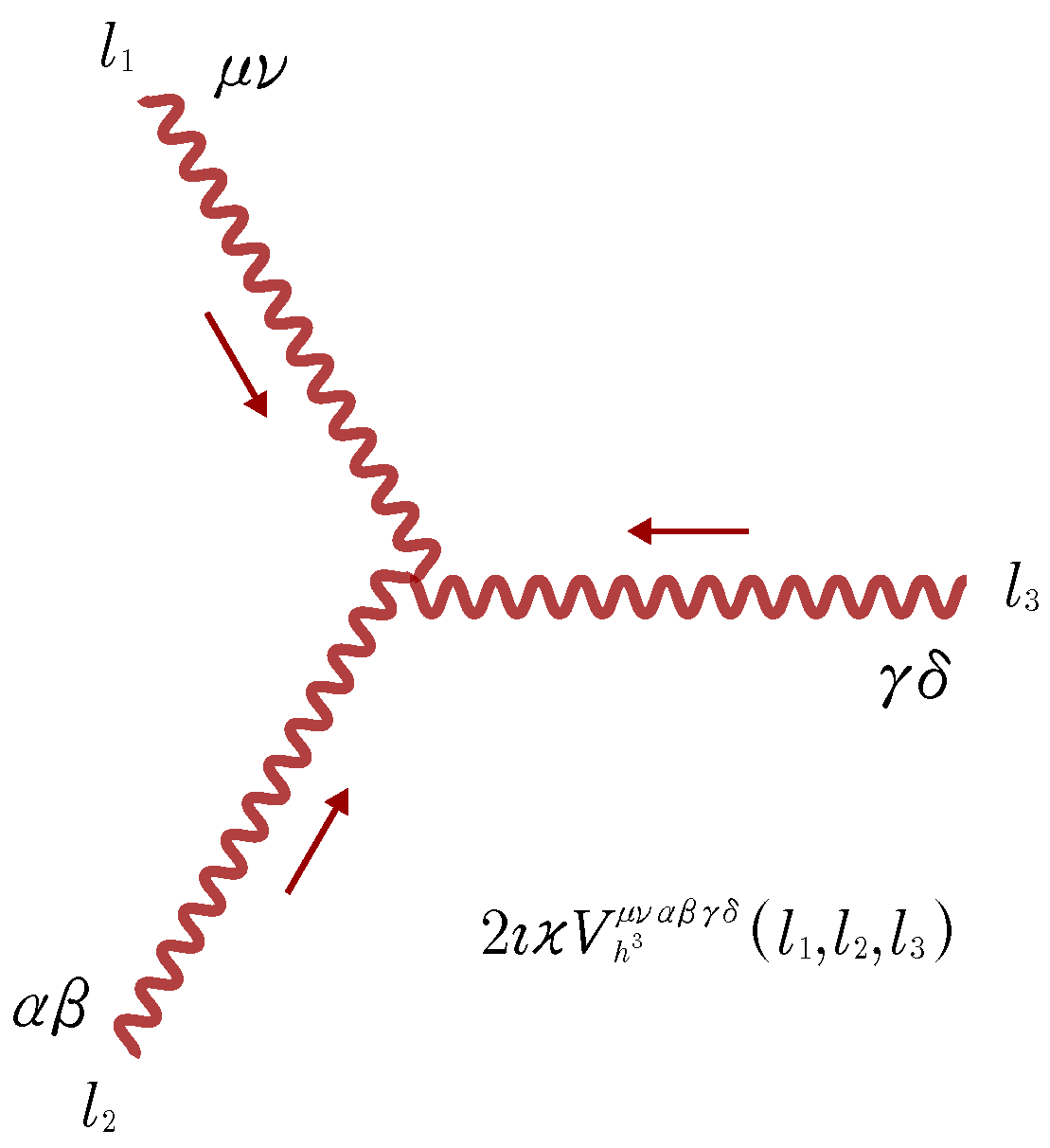
The graviton/graviton interactions are extremely complex. And as QGR is a non-linear gauge theory we have to include ghost terms in the action, which adds considerably to the complexity. DeWitt [38] notes there are 171 terms in the three point vertex, 2850 terms in the four point vertex – although he goes on to reassure us that with appropriate symmetrizations these may be reduced to 11 and 28 respectively.

Fortunately for our purposes here we do not actually need the details of the vertexes; we need their symmetry properties and how they scale with momentum, but the detailed index structure of the vertexes is the same in QGR and TGR, so not itself a concern.

We will look only at the three point vertex.

And we will focus on the case where there is no matter nearby and we are using a locally flat metric.

In SGR each vertex is accompanied by a

δ

function in three momentum plus a

δ

function in clock energy reflecting the fact that it is normal to take the limit as

τ \to \pm \infty

in SGR. Using the convention that all momenta are inward bound we have:

δ^{4} (l_{1} + l_{2} + l_{3})

(4.31)

The vertex is given (in Jakobsen’s notation) by:

2 ı κ V_{h^{3}}^{μ ν α β γ δ} (l_{1}, l_{2}, l_{3})

(4.32)

We have one pair of indices –

(μ ν) (α β) (γ δ)

for each incoming graviton. The vertex may be expanded out in terms of “U” functions. The U functions are complex but not functions of the momenta; they are eight dimensional constant matrices. In a certain sense the U function appears only once here; the second and third terms are symmetrized versions of the first. Each of the three terms gives up six of its eight indexes to the incoming gravitons, leaving the other two to pair with all three possible pairs of the graviton momenta.

V_{h^{3}}^{μ ν α β γ δ} (l_{1}, l_{2}, l_{3}) = - (U^{μ ν α β ρ γ δ σ} l_{(2) σ} l_{(3) ρ} + U^{α β γ δ ρ μ ν σ} l_{(3) σ} l_{(1) ρ} + U^{γ δ μ ν ρ α β σ} l_{(1) σ} l_{(2) ρ})

(4.33)

Note that the vertex is completely symmetric in its three inputs. And that there are two powers of

l^{2}

present. This latter is consistent with the fact that for gravity, energy is charge.

This is also the source of the difficulties with renormalization: the two extra powers of momentum in the numerator make the use of standard renormalization techniques difficult. For instance a standard loop integral might have two vertices. Each will contribute two extra powers of the momenta, making the loop integral not logarithmically divergence but quartically divergent.

In TQM the vertex structure is, as it was with QED, identical. The

δ

functions in momentum are adjusted just as they are in TQM: every vertex gets a

δ^{4}

in the coordinate energy and three momenta; it will have a

δ

in the clock energy if we are taking the limit as

τ \pm \infty

, otherwise not.

4.6. Feynman Rules for Metric and Matter

We now have all we need to write the Feynman diagrams for TGR. We assume we start with a set of Feynman diagrams for QGR. The topology and symmetries are the same as with QGR. All non-graviton parts are unchanged from TQM.

4.6.1. Initial Graviton Wave Function

The initial graviton wave functions have to be written with four rather than three dimensions 3.2. We can estimate the extension in energy for an individual wave function using the method in 2.1.7. The polarization part is unchanged.

We repeat for convenience:

SGR wave function:

G_{k}^{r} (τ, \vec{x}) = \frac{1}{\sqrt{2 V ω_{\vec{k}}}} H_{k}^{r} e^{- ı ω_{\vec{k}} τ + ı \vec{l} \cdot \vec{x}}

(4.34)

goes to TQM wave function:

G_{k}^{r} (t, x) = \frac{1}{\sqrt{2 TV u}} H_{k}^{r} e^{- ı ϖ_{k} τ - ı l x}

(4.35)

4.6.2. Graviton Propagator

The index part of the QGR propagator stays the same. For instance if the index factor is:

(δ_{μ α} δ_{ν β} + δ_{μ β} δ_{ν α} - δ_{μ ν} δ_{α β})

(4.36)

it stays unchanged. The spin zero factor maps in the same way that does in QED:

\frac{1}{k^{2} + ı ε} \to (\frac{exp (- ı ϖ_{k} τ)}{2 w} θ (τ) - \frac{exp (- ı ϖ_{k} τ)}{2 w} θ (- τ))

(4.37)

4.6.3. Vertexes

The vertexes are unchanged except that the accompanying delta function is changed per the above: the vertex gets an addition

δ

function in the coordinate energy while the

δ

function in clock energy is deprecated and rare.

4.6.4. Overall Diagram

The same remark applies to the

δ

functions in overall momenta.

We allow for short times:

δ (Σ u_{i n} - Σ u_{o u t}) \to \int_{τ_{s t a r t}}^{τ_{f i n i s h}} d τ exp (- ı ϖ_{l} τ)

(4.38)

but expand the remaining three dimensional overall delta functions into four dimensional delta functions:

δ^{3} (Σ {\vec{l}}_{i n} - Σ {\vec{l}}_{o u t}) \to δ^{4} (Σ l_{i n} - Σ l_{o u t})

(4.39)

4.6.5. Discussion

With that caveat, the main objective of this paper is accomplished. We can take any SGR Feynman diagram and translate it into an equivalent TGR diagram. It will include paths in time on the same basis as paths in space. And the loops will be convergent.

While we can compute any Feynman diagram in principle as a practical matter the combinatoric explosion in indexes requires the use of dedicated software. An appropriate starting point may be provided by the open source Mathematica packages FeynGrav, FeynCalc, FeynArts [62,63,64,65,66,67,95,96,143,144,145,146].

The methods used to distinguish between SQM and TQM in the QED arena will not work here: those methods looked for differences at the attosecond scale. This scale looks to be well below the reach of any currently proposed tests of QGR. Therefore we are unlikely to be able to find a direct test that distinguishes between SGR and TGR. In the section Experimental and Observational Tests we will look at indirect tests.

5. Self-Energy Calculation for Gravitons

“The shell game that we play … is technically called ’renormalization’. But no matter how clever the word, it is still what I would call a dippy process! Having to resort to such hocus-pocus has prevented us from proving that the theory of quantum electrodynamics is mathematically self-consistent. It’s surprising that the theory still hasn’t been proved self-consistent one way or the other by now; I suspect that renormalization is not mathematically legitimate.” - Richard P. Feynman p128 [57]

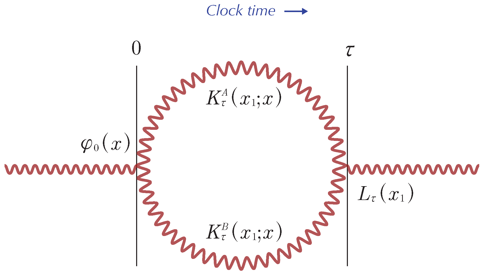
Figure 4. Simple loop diagram.

The loop integrals in QED have been a problem since its inception. They are dealt with by renormalizing, by comparing two “nearby” integrals and arguing that even if each is infinite, it is only the difference between the two that is physically significant. It then is possible to combine integrals in such a way that all measurable properties are finite.

We originally expected that the loop diagrams would be still more of a problem in TQM: TQM has one more dimension to integrate over in the loop integrals: we would expect that the loop diagrams might go from logarithmically divergent to linearly divergent, perhaps making them unrenormalizable. More detailed calculations, however, showed that two factors:

initial finite dispersion in time
entanglement in time

made the loop diagrams self-regularizing. This is essentially the same mechanism that guaranteed the convergence of the time slice integrals in the non-relativistic case. Of course the calculations in the field theory case are much more complex.

5.1. Loop Calculation

We will first calculate the loop for fixed clock time, then take the Fourier transform of this with respect to clock time. This functions as an effective mass correction. The details of how that is done are familiar; our goal here is show that the loop and the Fourier transform of the loop with respect to clock time are finite in TGR. The graviton splits into two at clock time

τ = 0

. Each of the two gravitons travels along till time

τ

, when they merge. The loop is normally calculated in momentum space, but in some ways the calculation is clearer in coordinate space. We have:

L_{τ} (x_{1}) = - κ^{2} \int d^{4} x K_{τ}^{A} (x_{1}; x) K_{τ}^{B} (x_{1}; x) φ_{0} (x)

L represents the wave function as it is modified by the loop. It will be added to the initial wave function to get the loop corrected wave function. To get the full loop correction we will need to sum over clock time. To do this we will take the Fourier transform with respect to the clock time. But we will focus on the loop correction at fixed clock time first.

We will take the wave function as a Gaussian. If it is a Gaussian in coordinate space it is also one in momentum space and vice versa.

The basic idea is to observe that if we take the initial wave function as a Gaussian in four dimensions, each of the four Gaussians serves to regularize one of the four loop integrals. The regularization is supplied by the incoming wave function. In coordinate space this is obvious, but the QGR vertex functions are unmanageable in coordinate space. So we will shift back and forth at need.

Note that in standard field theory this does not work: connecting the time/energy part of the initial wave function to the time/energy variable in the integral is exactly entanglement in time. And entanglement-in-time is one aspect of time-as-observable, a defining property of TQM, forbidden in QED.

5.1.1. Setup

Vertex

As noted earlier, the three graviton vertex has six indexes. A simple loop has two of these:

2 ı κ V_{h^{3}}^{μ ν α β γ δ} (l_{1}, l_{2}, l_{3})

(5.1)

In each vertex the three incoming momenta occur in pairs:

l_{1}, l_{2}

and

l_{2}, l_{3}

and

l_{3}, l_{1}

in a fully symmetric manner. In the case of our loop the incoming momentum is p and the loop momentum is k. Each vertex contains two momenta in symmetric pairs. At each vertex the pairs are

p, k

p, p - k

k, p - k

. The external momenta p is fixed, so that momenta that are integrated over as part of the loop go as the powers of k from

0 \to 4

. Depending on the specifics we might be looking at

w^{2} k_{x}

in one term and

w^{4}

at another and so on. The total number of k factors in a single term is a maximum of 4. As noted, DeWitt put the number of terms at each three vertex at 171 so that the total number of our terms here is 29241. DeWitt shows that the number of distinct terms is much smaller, but the loops in QGR are still far more complex than those in QED.

Initial Wave Function

We estimate the initial wave function as a Gaussian with fixed dispersions in energy and momentum.

φ_{0} (p) = \sqrt[4]{\frac{1}{π^{4} det (\hat{Σ})}} e^{ı {(p - p_{0})}_{μ} x_{0}^{μ} - {(p - p_{0})}^{μ} \frac{1}{2 {\hat{Σ}}^{μ ν}} {(p - p_{0})}^{ν}}

(5.2)

We take the initial dispersion as diagonal in the momentum. Effectively the initial wave function is a product of four separate Gaussians in

E, p_{x}, p_{y}, p_{z}

\hat{Σ} \equiv (\begin{matrix} {\hat{σ}}_{t} & 0 & 0 & 0 \\ 0 & {\hat{σ}}_{x}^{2} & 0 & 0 \\ 0 & 0 & {\hat{σ}}_{x}^{2} & 0 \\ 0 & 0 & 0 & {\hat{σ}}_{z}^{2} \end{matrix})

(5.3)

As noted earlier, using Morlet wave analysis any normalizable wave function may be written as sums over such direct products, so there is no loss of generality in doing this.

The equivalent wave function in coordinate space is very similar:

φ_{0} (x) = \sqrt[4]{\frac{1}{π^{4} det (\hat{Σ})}} e^{- ı p_{0 μ} x^{μ} - {(x - x_{0})}^{μ} \frac{1}{2 Σ^{μ ν}} {(x - x_{0})}^{ν}}, Σ = \frac{1}{\hat{Σ}}

(5.4)

Propagator

The propagators are much simpler in momentum space:

\begin{matrix} K^{S} (k) = \frac{ı}{k^{2} - μ^{2} + ı ε} \to K_{τ}^{T} (k) = \frac{exp (- ı ϖ_{k} τ)}{2 w} θ (τ) \\ ϖ_{k} \equiv - \frac{k^{2}}{2 w}, k^{2} = w^{2} - {\vec{k}}^{2} \end{matrix}

(5.5)

Note we have shifted from the Feynman boundary conditions to retarded boundary conditions. The kernels are shorthand for:

\hat{K} (k) \to \hat{K} (k_{1}; k) δ^{4} (k_{1} - k)

(5.6)

The propagators in coordinate space are much more complex. In the non-relativistic case, the momentum space propagator replaces the factors of the relativistic energy with the rest mass:

\frac{1}{2 w} \to \frac{1}{2 m}

(5.7)

With this change the kernel in coordinate space is:

K_{τ} (x; x^{'}) = - ı \frac{m_{0}^{2}}{4 π^{2} τ^{2}} e^{- ı m_{0} \frac{{(t - t^{'})}^{2}}{2 τ} + ı m_{0} \frac{{(\vec{x} - {\vec{x}}^{'})}^{2}}{2 τ} - ı \frac{m_{0}}{2} τ}

(5.8)

If we use steepest descents to approximate the coordinate kernel, given the exact momentum space kernel, we can expand:

\frac{1}{2 w} \to \frac{1}{2 w_{0}} (1 - \frac{δ w}{w_{0}} + \frac{δ w^{2}}{w_{0}^{2}} - \dots), w = w_{0} + δ w

(5.9)

More generally we could write:

k = k_{0} + δ k

(5.10)

Then we get the steepest descents approximation by expanding around

k_{0}

to second order in

δ k

. We are going to further simplify by approximating the denominators to zeroth order, i.e. just the average energy. This let us treat the kernel in coordinate space as the product of four independent kernels, one for each dimension.

This is a technical change; we could if we wished expand the denominators to second order. The cost would be a slight correction to the time-squared part of the argument, which would not be too bad, and cross terms in

δ w δ k_{x}

, which we could get rid of by diagonalizing the argument. Since our goal is only to show the integrals are finite, not to compute their most exact values, we keep the simpler if less accurate form.

Core Loop Calculation

We now take advantage of the symmetry of the loop calculation in the case of graviton. This is one of the few places where a calculation in quantum gravity is simpler than the equivalent calculation in QED. Consider a graviton with average momentum:

p_{0} = (E_{0}, {\vec{p}}_{0})

(5.11)

It splits into two gravitons. The best estimate of the relativistic energy for each is half of the article-title energy:

E_{1} = \frac{E_{0}}{2}

(5.12)

Since there are two gravitons and their kernels are identical, the total kernel to go from

x \to x_{1}

is:

K_{τ}^{(e f f)} (x; x^{'}) = - ı \frac{E_{0}^{2}}{16 π^{2} τ^{2}} K_{τ} (x; x^{'})

(5.13)

We can write the equivalent momentum space kernel by inspection:

{\hat{K}}_{τ}^{(e f f)} (p; p^{'}) = - ı F_{τ} {\hat{K}}_{τ} (p; p^{'}), F_{τ} \equiv \frac{E_{0}^{2}}{16 π^{2} τ^{2}}

(5.14)

Or more explicitly:

{\hat{K}}_{τ}^{(e f f)} (p; p^{'}) = - ı F_{τ} \frac{exp (- ı ϖ_{p} τ)}{2 E} δ^{4} (p - p')

(5.15)

We are free to replace the E in the denominator with

E_{0}

and cancel it against one of the

E_{0}

’s in the numerator if we wish.

We got a similar result in the mass correction loop in the QED case, the

F_{τ}

there was:

- ı \frac{m^{2}}{4 π^{2} τ^{2}}

(5.16)

With the replacement

m \to \frac{E_{0}}{2}

the overall factor is the same. The clock frequency was not as simple, however.

Fourier Transform

The Fourier transform of the kernel is given by:

F T [\frac{exp (- ı ϖ_{p} τ)}{τ^{2}}] = - \sqrt{\frac{π}{2}} |ω - ϖ_{p}|

(5.17)

so the loop correction is:

{\hat{L}}_{ω} (p) = ı \frac{E_{0}^{2}}{16 π^{2}} \sqrt{\frac{π}{2}} |ω - ϖ_{p}^{M}|

(5.18)

Quadratic and Higher Powers of the Momentum

Whereas in QED or in standard QGR the regularizing factor has to be supplied by hand, in TQM and TGR it is supplied by the initial wave function. Any mere polynomial potential will be easily regularized by the wave function. We have been using Gaussians for convenience but as noted these are completely general.

We can do the actual calculations with this same approach here provided we are willing to be a bit more careful about our steepest descents approximation. If we add an additional factor of, say:

exp (- ı α_{μ} k^{μ})

(5.19)

in the definition of the momentum space kernel, and then do the steepest descents calculation in detail, at the end of the calculation we can take the derivative of the result with respect to

α_{μ}

to get whatever powers of the momentum we need to see integrated over:

{- ı \frac{\partial}{\partial α_{μ}} K^{e f f e c t i v e}|}_{α_{μ} = 0} \to K^{e f f e c t i v e} (k^{μ})

(5.20)

Higher powers means more derivatives. As they are being compared to Gaussians, the degree of the polynomial will not make the integral infinite.

5.2. Discussion

5.2.1. If Renormalization Does not Make Sense, Why Does It Work So Well?

The most obvious question about renormalization is “why does it work at all?” As Feynman (among many others) noted it does not make sense. Yet it works astonishingly well.

The approach here sheds some light on this. The effective regularization function is the time dispersion of the initial wave function. Renormalization works by looking at the difference between the loop calculation at two different starting points. If these starting points have initial wave functions with similar dispersions in time, the correction due to the difference in the these two regularization functions will be a correction to a correction, and therefore quite possibly too small to see.

5.2.2. Could We See the Effects of Regularization in TGR?

At sufficiently high energies, we should see the effects of the regularization function take effect. In principle, these functions are then detectable.

We would almost certainly need something more finely calibrated than the maximum entropy estimate of the dispersion in time that we started with. That makes sense in terms of giving an order-of-magnitude estimate. And that in turn should be adequate for falsifiability. But it is not likely to be suitable for precision work.

It would be preferable to have an a priori estimate of the initial wave function in time. In QED, we would need to compute the bound state wave functions with time now part of the calculation. This looks doable but non-trivial. Once this is done we could look at, say, the Lamb shift and see what further corrections would result from differences in the dispersion in time for the

2 s

and the

2 p

states that are compared there.

In TGR we would need to work out the statistical mechanics of an ensemble of gravitons, as that would be the population an incoming graviton would be coming from. This is also non-trivial.

6. Experimental and Observational Tests

“In this work, the potential of twisted light for the generation of gravitational waves in the high frequency regime is explored for the first time. ... Compelling evidence is provided that the properties of the generated gravitational waves, such as frequency, polarisation states and direction of emission, are controllable by the laser pulse parameters and optical arrangements.” – Atonga et al [11]

The fundamental problem in developing tests of quantum gravity is that gravitons, if they exist, do not couple strongly to matter. See Rothman [130] and also Nicolini [106].

Graviton/Photon Hybrids

We discussed previously the possibility that under the right conditions graviton-photon hybrids might form. The force between the two halves would go as the product of their energies so the optimal conditions for the production would be conditions where high energy gravitons and photons are created simultaneously. The collapse of two neutron stars into each other is one possibility (as in the GW170817 gravitational wave detection [118]). The work of Atonga et al [11] is another. This is focused on the use of intense laser beams to generate gravitational waves. One asks if the same approach could be used to generate gravitons and/or graviton-photon pairs? The great advantage of such pairs is that the photon half of the hybrid would be relatively detectable. From our specific point of view, these may also serve as tests of TGR since there will almost certainly be a strong time element.

Gravity as a Classical Potential with Effects on Quantum Particles

In a number of the proposed experiments the effects of gravity are similar to the effects of any other (classical) potential. For instance in the Overstreet treatment of the Aharonov-Bohm effect from a gravitational field [117] the passage through a gravity potential changes the relative phase of the two halves of the wave function. An interferometer can then detect the difference. The same sort of thing is predicted from gravitational time dilation [131].

In semi-classical approximation, the phase goes as the integral of the Lagrangian along the path, i.e. the action. Different paths give different values of the action, hence interference effects. Unfortunately as TGR uses the GR action, the actions along the paths are going to be the same. Such approaches do not seem promising as tests of TGR specifically, although they are interesting in their own right.

Gravity as a Quantum Field

The next step up in sophistication is to see gravity as a quantum field and look specifically for effects that are only present at the quantum level. Entanglement is one such; see discussions in [19,126]. One could also look for interference between different quantum states of spacetime, as in [32].

Unless the entanglement involves entanglement in time, such experiments are unlikely to disambiguate between TGR and standard QGR.

The Metric as an Ensemble of Gravitons

Decoherence has been proposed as a mechanism to help explain the transition from the quantum to the classical case [85,109,137,174,175,180,181,182,183,184,185]. Gravity is particularly attractive as a source of decoherence; it is omnipresent and can therefore explain why most of the observable universe appears to be made of classical objects. A number of experiments have been proposed to look for decoherence effects created by gravity [3,5,13,14,17,26,99,120,121,122,128,136,165,171].

When decoherence is used to model the collapse of the wave function it invariably is modeling the loss of information from the observed system. Since in quantum mechanics information can neither be created nor destroyed (see the no-cloning and no-deleting theorems), the information must have gone somewhere. That somewhere is always the system doing the detecting. And that system has to be modeled as a statistical system. In this way, we ensure that the “lost” information is still extant but no longer accessible, it is “lost in the crowd”.

Specific examples of decoherence generally need to model the statistical mechanics of the system doing the decohering.This makes them the first of these classes of experiments which can specifically be used to test for TGR as opposed to QGR. This is sufficiently important here that we devote the next section to it.

7. Statistical Mechanics of the Graviton Ensemble

We look at the statistical mechanics of the graviton ensemble. We are not going to work out the rules for this here; it is a large, complex subject requiring a dedicated investigation. Instead we are going to discuss why we should make such an investigation, how we can go about this, and how we might compare the predictions of TGR to currently available observations.

We start with two working hypotheses:

that the GR metric is in fact composed of a statistical ensemble of gravitons.
and that the metric acts as a store of energy and information.

Metric as a Statistical Ensemble of Gravitons

Jakobsen [84] has shown that we can derive the Schwartzschild metric from QGR, which is strong evidence of the feasibility of this approach. He and Latosh [95,96] both cite a significant literature developing general relativity from a particle perspective. It appears that there is no fundamental principle barring this approach, even if it is a minority view.

See also the discussion in [60] of gravity as irreversible, a statistical property.

Treating the metric as an ensemble of gravitons provides a natural explanation of the black hole information paradox [69,108,150]: as with decoherence, information that goes into a black hole is not lost, it has merely been “misplaced”, part of the sea of gravitons that comprises the metric, even the black hole metric.

Metric as a Store of Energy and Information

There has been a fair amount of work on the energy to be associated with spacetime: Weinberg [169], Dirac [41], and Baryshev has a review of this [12]. Baryshev discusses the storage of energy in the gravity field. We have not seen a discussion of the storage of energy and information in the metric treated as a statistical system.

There is some indirect evidence to suggest the metric should be treated as a statistical system, and further one with its own characteristic properties. The cosmic microwave background (CMB) currently has an estimated energy density of

0.260 e V / c m^{3}

0.260 M e V / m^{3}

[170]. The cosmological constant corresponds to an energy density of about

3.35 G e V / m^{3}

[125]. Naively, the statistical structure of graviton gas should be very similar to that of a photon gas; they are both massless and there are two degrees of freedom. We may reasonably assume that being, as it were, in very close proximity, they are at the same temperature. The gravitons have an attractive force for each other, but that is normally considered weak. If we model the graviton gas using the same approach as for the photon gas ([30]) then for the gravitons to have a heat capacity about 12,000 times greater than a photon gas is a discrepancy too great to easily reconcile.

In statistical mechanics we normally weight each state by with an occupation number of n and momentum

\vec{k}

by:

exp (- β n |\vec{k}|)

(7.1)

where

β \equiv \frac{1}{k T}

When time is an observable we are at liberty to look at off-shell variation, as:

exp (- β n |\vec{k}| - n \frac{{(w - |\vec{k}|)}^{2}}{2 σ_{k}^{2}})

(7.2)

where the dependence on w is a Gaussian centered on

|\vec{k}|

. If

σ_{|\vec{k}|}^{2}

is small enough, this turns into a

δ

function so reduces to the usual.

This provides an adjustable constant in the dispersion in energy. It can easily account for the factor of 12,000 difference. Too easily in fact, which is a problem.

Feynman and Hibbs [58] show we can use Feynman path integrals to compute partition functions. The core of the approach is to note the formal resemblance between partition functions and the path integral, then exploit this resemblance by using imaginary time as formally equivalent to a temperature. This should let us compute the partition function for a graviton ensemble from first principles.

Could a graviton gas be that different in character from a photon gas? The force between gravitons is attractive and for gravity the energy of the graviton functions as charge. A statistical distribution with an otherwise disproportionately high percentage of high energy gravitons might be energetically favored because of the potential energy benefits.

How this plays out is best determined by detailed calculation. If a formal calculation is consistent with the dark energy energy density, then we will have confirmatory evidence. If it does not, we will have falsified the hypothesis.

Decoherence Experiments as a Probe of the Graviton Ensemble

The decoherence experiments discussed previously necessarily probe the statistical structure of the gravitons. For instance, high energy photons will couple at one rate, lower energy at another. The results from such experiments may be used to probe the statistical structure of the gravitons.

Metric as Explanation of Dark Energy and Dark Matter

We currently detect dark energy and dark matter only through their gravitational effects, through the metric. While many explanations have been proposed for them, none have been confirmed.

It is possible that the explanation for these two phenomena is that they represent an accumulation of energy in the metric structure of spacetime. Dark energy would be the part averaged over the universe, dark matter would be the local variations in the energy distribution.

Normally in general relativity we assume that the exchange of energy and momentum between metric and matter is entirely described by the Einstein equations “Space tells matter how to move Matter tells space how to curve” (Wheeler in [101]). But as noted, QGR implies an additional mechanism for the exchange of energy and information between matter and metric, a kind of quantum friction.

If the metric is correctly described as an ensemble of gravitons, then these transfers will be governed by the principles of statistical mechanics. Now consider the situation at the Big Bang. Assume there is relatively little energy in the metric. We expect then that there will be a transfer of energy from matter to metric. This will result in an increase in the temperature and the volume of the metric, in other words it will look like an expansion of the universe (i.e. dark energy). Once the universe has expanded enough that its parts are no longer in effective communication with each other the rate of transfer will be governed by local conditions. Any concentrations of energy in matter (i.e stars and galaxies) will drive transfers of energy into the local metric (i.e. dark matter). The transfers of this energy within the metric will look like currents of energy radiating outward from the core of a galaxy, surrounding galaxies with a halo of dark matter.

The patterns of the initial transfer and the local transfers will obey the rules of statistical mechanics. The direction of the transfer of energy from matter to metric or vice verse will be determined by whichever transfer increases entropy the most. The rate will be defined by the coupling matrices, integrated over the local metric and matter.

Observations of the history of dark energy and dark matter will provide an additional line of attack on the partition function of the metric.

Falsifiability

We have a way to compute the statistical structure of graviton ensemble and several ways to compare the predicted structure with experimental and observational evidence. Therefore TGR is falsifiable in principle.

8. Discussion

The question of whether time should be treated as a parameter or as an operator goes back to the start of quantum mechanics. Heisenberg [71] took for granted that it should, at least in the sense that the uncertainty principle should apply to the time/energy relation as it does to the space/momentum relation. But practice since then has largely treated time as a parameter. Our initial goal was to force the issue and see what breaks.

The push to non-relativistic quantum mechanics and then to QED was relatively straightforward: with Feynman path integrals it was largely a matter of extending the paths to include motion in the future/past direction on the same basis as motion in the right/left, forward/back, and up/down directions. For the most part the rest of the FPI machinery could be left untouched.

This can be seen as an exercise of Wheeler’s principle of radical conservatism: we are taking both special relativity and quantum mechanics completely seriously. By making time an operator we are merely “completing the square”. The predictions are well-defined; the associated tests non-trivial but feasible with current technology. We expect that TQM will be confirmed/falsified in the near future.

What we have done in this paper is apply the same approach to quantum general relativity: we have combined not special relativity but general relativity with quantum mechanics, again taking both completely seriously. The non-linear character of general relativity and the presentation of general relativity as curvature in spacetime present technical problems. But the use of the metric as the field to be quantized lets us use the same procedures for general relativity as we had used for QED.

Further we have shown here that the UV divergences are contained in QGR just as they are contained in QED. In fact, for once, the calculations in QGR were simpler than in QED. With this we established that TGR is a renormalizable model for QGR.

It is not yet established that general relativity should be quantized in the first place. However if it should be quantized then it is very difficult to see how that could be done correctly without quantizing time and the three space dimensions in the same way and at the same point in the calculation. In a way then, and a bit paradoxically, any confirmation of QGR – whether or not the confirmation is specifically of time-related aspects of QGR – will tend to confirm that time should be treated as an operator in QM as well. Of course as a practical matter we would expect to see confirmations with QM first.

The predictions for TGR are well-defined if technically demanding to work out. The next question is: are the odds good enough to justify the potentially significant effort required to test the predictions by observation or experiment?

TGR starts from well-defined and accepted theories – general relativity and QED – and combines them in a straight-forward way. Further it does not suffer from the infinities that trouble SGR. Therefore the odds of confirmation should be reasonably good.

As additional motivation, the necessary experiments tend to be interesting in their own right. For instance, to compare the predictions of TGR for the graviton ensemble with nature using decoherence we need to look at decoherence probes of spacetime in a different way: not just is there decoherence? but how fast does it happen? at different frequencies? is there latency? does a quantized spacetime give us a way to entangle matter at different locations? and so on.

To compare those predictions with observations of dark energy and dark matter we need to think about those mysterious phenomena in a different way: what is their history? are stars and galaxies interacting with spacetime at the thermodynamic level? or is it curvature all the way down? and so on.

In a certain sense, an experimental or observational test of time-as operator is likely to have no null outcomes; whatever result comes back, that result should tell us something interesting about nature. Which is ultimately the goal.

Acknowledgments

I thank my long time friend Jonathan Smith for invaluable encouragement, guidance, and practical assistance. I thank Ferne Cohen Welch for extraordinary moral and practical support. I thank Martin Land, L. P. Horwitz, James O’Brien, Tepper Gill, Petr Jizba, Matthew Trump, and the other organizers of the International Association for Relativistic Dynamics (IARD) 2018, 2020, and 2022 Conferences for encouragement, useful discussions, and hosting talks on the papers in this series in the IARD conference series. I also thank my fellow participants in the 2022 conference – especially Pascal Klag, Bruce Mainland, Luca Smaldone, Howard Perko, Philip Mannheim, Alexey Kryukov, Ariel Edery, and others – for many excellent questions and discussions. I thank Steven Libby for several useful conversations and in particular for insisting on the extension of the article-title ideas to the high energy limit and therefore to QED. I thank Avi Marchewka for an interesting and instructive conversation about various approaches to time-of-arrival measurements. I thank Asher Yahalom for insisting that a better explanation of the clock time than simply what clocks measure was required. I thank Y. S. Kim for organizing the invaluable Feynman Festivals, for several conversations, and for general encouragement and good advice. I thank Walt Mankowski for useful questions I thank Arthur Tansky for useful questions. I note he independently suggested the approach developed here. And I note that none of the above are in any way responsible for any errors of commission or omission in this work.

References

A. Addazi, J. Alvarez-Muniz, R. Alves Batista, G. Amelino-Camelia, V. Antonelli, M. Arzano, M. Asorey, J.-L. Atteia, S. Bahamonde, F. Bajardi, A. Ballesteros, B. Baret, D.M. Barreiros, S. Basilakos, D. Benisty, O. Birnholtz, J.J. Blanco-Pillado, D. Blas, J. Bolmont, D. Boncioli, P. Bosso, G. Calcagni, S. Capozziello, J.M. Carmona, S. Cerci, M. Chernyakova, S. Clesse, J.A.B. Coelho, S.M. Colak, J.L. Cortes, S. Das, V. D’Esposito, M. Demirci, M.G. Di Luca, A. di Matteo, D. Dimitrijevic, G. Djordjevic, D. Dominis Prester, A. Eichhorn, J. Ellis, C. Escamilla-Rivera, G. Fabiano, S.A. Franchino-Viñas, A.M. Frassino, D. Frattulillo, S. Funk, A. Fuster, J. Gamboa, A. Gent, L.Á. Gergely, M. Giammarchi, K. Giesel, J.-F. Glicenstein, J. Gracia-Bondía, R. Gracia-Ruiz, G. Gubitosi, E.I. Guendelman, I. Gutierrez-Sagredo, L. Haegel, S. Heefer, A. Held, F.J. Herranz, T. Hinderer, J.I. Illana, A. Ioannisian, P. Jetzer, F.R. Joaquim, K.-H. Kampert, A. Karasu Uysal, T. Katori, N. Kazarian, D. Kerszberg, J. Kowalski-Glikman, S. Kuroyanagi, C. Lämmerzahl, J. Levi Said, S. Liberati, E. Lim, I.P. Lobo, M. López-Moya, G.G. Luciano, M. Manganaro, A. Marcianò, P. Martín-Moruno, Manel Martinez, Mario Martinez, H. Martínez-Huerta, P. Martínez-Miravé, M. Masip, D. Mattingly, N. Mavromatos, A. Mazumdar, F. Méndez, F. Mercati, S. Micanovic, J. Mielczarek, A.L. Miller, M. Milosevic, D. Minic, L. Miramonti, V.A. Mitsou, P. Moniz, S. Mukherjee, G. Nardini, S. Navas, M. Niechciol, A.B. Nielsen, N.A. Obers, F. Oikonomou, D. Oriti, C.F. Paganini, S. Palomares-Ruiz, R. Pasechnik, V. Pasic, C. Pérez de los Heros, C. Pfeifer, M. Pieroni, T. Piran, A. Platania, S. Rastgoo, J.J. Relancio, M.A. Reyes, A. Ricciardone, M. Risse, M.D. Rodriguez Frias, G. Rosati, D. Rubiera-Garcia, H. Sahlmann, M. Sakellariadou, F. Salamida, E.N. Saridakis, P. Satunin, M. Schiffer, F. Schüssler, G. Sigl, J. Sitarek, J. Solà Peracaula, C.F. Sopuerta, T.P. Sotiriou, M. Spurio, D. Staicova, N. Stergioulas, S. Stoica, J. Strišković, T. Stuttard, D. Sunar Cerci, Y. Tavakoli, C.A. Ternes, T. Terzić, T. Thiemann, P. Tinyakov, M.D.C. Torri, M. Tórtola, C. Trimarelli, T. Trześniewski, A. Tureanu, F.R. Urban, E.C. Vagenas, D. Vernieri, V. Vitagliano, J.-C. Wallet, and J.D. Zornoza. Quantum gravity phenomenology at the dawn of the multi-messenger era—a review. Progress in Particle and Nuclear Physics, 125:103948, 2022, 2111.05659.
Ronald Adler, Maurice Bazin, and Menahem Schiffer. Introduction to General Relativity. McGraw-Hill, New York, 1965.
Eissa Al-Nasrallah, Saurya Das, Fabrizio Illuminati, Luciano Petruzziello, and Elias C. Vagenas. Discriminating quantum gravity models by gravitational decoherence. ArXiv e-prints, 10 2021, 2110.10288.
Pascal Anastasopoulos, Kunio Kaneta, Yann Mambrini, and Mathias Pierre. Energy-momentum portal to dark matter and emergent gravity. Phys. Rev. D, 102:055019, 2020, 2007.06534. [CrossRef]
C. Anastopoulos and B. L. Hu. A master equation for gravitational decoherence: Probing the textures of spacetime. ArXiv e-prints, May 2013, 1305.5231v3. Class. Quantum Grav. 30 165007 (2013). [CrossRef]
Arto Annila and Mårten Wikström. Dark matter and dark energy denote the gravitation of the expanding universe. Frontiers in Physics, 10, 2022. [CrossRef]
John Ashmead. Time dispersion in quantum mechanics. Journal of Physics: Conference Series, 1239:012015, May 2019.
John Ashmead. Does the Heisenberg uncertainty principle apply along the time dimension? Journal of Physics: Conference Series, 1956(1):012014, 2021, 2101.10512.
John Ashmead. Time dispersion in quantum electrodynamics. Journal of Physics: Conference Series, 2482(1):012023, may 2023.
Markus Aspelmeyer. How to avoid the appearance of a classical world in gravity experiments. ArXiv e-prints, 03 2022, 2203.05587.
Eduard Atonga et al. Gravitational waves from high-power twisted light. ArXiv e-prints, 9 2023, 2309.04191.
Yu. V. Baryshev. Energy-momentum of the gravitational field: Crucial point for gravitation physics and cosmology. ArXiv e-prints, 2008, 0809.2323.
Angelo Bassi, André Großardt, and Hendrik Ulbricht. Gravitational decoherence. Class. Quantum Grav., 34:193002, 2017, 1706.05677.
Sayantani Bera, Sandro Donadi, Kinjalk Lochan, and Tejinder P. Singh. A comparison between models of gravity induced decoherence. ArXiv e-prints, Aug 2014, 1408.1194v2.
Per Berglund, De-Chang Dai, Douglas Edmonds, Yang-Hui He, Tristan Hubsch, Vishnu Jejjala, Michael J. Kavic, Djordje Minic, Samuel Powers, John H. Simonetti, Dejan Stojkovic, and Tatsu Takeuchi. Quantum gravity and phenomenology: Dark matter, dark energy, vacuum selection, emergent spacetime, and wormholes. ArXiv e-prints, 02 2022, 2202.05104.
Simeon Bird, Ilias Cholis, Julian B. Muñoz, Yacine Ali-Haïmoud, Marc Kamionkowski, Ely D. Kovetz, Alvise Raccanelli, and Adam G. Riess. Did ligo detect dark matter? Phys. Rev. Lett., 116:201301, 2016, 1603.00464.
M. P. Blencowe. Effective field theory approach to gravitationally induced decoherence. ArXiv e-prints, Dec 2012, 1211.4751v1. Phys. Rev. Lett. 111, 021302 (2013). [CrossRef]
Sougato Bose, Ivette Fuentes, Andrew A. Geraci, Saba Mehsar Khan, Sofia Qvarfort, Markus Rademacher, Muddassar Rashid, Marko Toroš, Hendrik Ulbricht, and Clara C. Wanjura. Massive quantum systems as interfaces of quantum mechanics and gravity. ArXiv e-prints, 2023, 2311.09218.
Sougato Bose, Anupam Mazumdar, Gavin W. Morley, Hendrik Ulbricht, Marko Toroš, Mauro Paternostro, Andrew Geraci, Peter Barker, M. S. Kim, and Gerard Milburn. A spin entanglement witness for quantum gravity. Phys. Rev. Lett., 119:240401, 2017, 1707.06050.
Tobias Bothwell, Colin J. Kennedy, Alexander Aeppli, Dhruv Kedar, John M. Robinson, Eric Oelker, Alexander Staron, and Jun Ye. Resolving the gravitational redshift across a millimetre-scale atomic sample. Nature, 602(7897):420–424, 2022. [CrossRef]
Dillon Brout, Dan Scolnic, Brodie Popovic, Adam G. Riess, Joe Zuntz, Rick Kessler, Anthony Carr, Tamara M. Davis, Samuel Hinton, David Jones, W. D’Arcy Kenworthy, Erik R. Peterson, Khaled Said, Georgie Taylor, Noor Ali, Patrick Armstrong, Pranav Charvu, Arianna Dwomoh, Antonella Palmese, Helen Qu, Benjamin M. Rose, Christopher W. Stubbs, Maria Vincenzi, Charlotte M. Wood, and Peter J. Brown. The pantheon+ analysis: Cosmological constraints. ApJ 938 110 (2022), 02 2022, 2202.04077.
Clare Burrage. A brief introduction to extended gravity and connections to dark energy: Illustrated with scalar field examples. SciPost Phys. Lect. Notes, page 41, 2022. [CrossRef]
P. Busch. The Time Energy Uncertainty Relation, pages 69–98. Lecture Notes in Physics. Springer-Verlag, Berlin, 2001.
Craig Callender. What Makes Time Special? Oxford University Press, 2017.
Craig Callender and Nick Huggett. Physics meets philosophy at the Planck scale: contemporary theories in quantum gravity. Cambridge University Press, Cambridge, UK ; New York, 2001.
Matteo Carlesso and Angelo Bassi. Decoherence due to gravitational time dilation: analysis of competing decoherence effects. Physics Letters A, Volume 380, Number 31-32, 2016, 02 2016, 1602.01979. [CrossRef]
Daniel Carney, Philip C. E. Stamp, and Jacob M. Taylor. Tabletop experiments for quantum gravity: a user’s manual. Classical and Quantum Gravity, Volume 36, Number 3, 2019, 07 2018, 1807.11494.
Sean Carroll. Something Deeply Hidden: Quantum Worlds and the Emergence of Spacetime. Dutton, 2022.
Sean M. Carroll. Spacetime and geometry: an introduction to General Relativity. Addison Wesley, San Francisco, 2019.
Ming Chen and Yong-Chang Huang. Gas model of gravitons with light speed. BJUT ITP01, 02 2014, 1402.5767.
Marios Christodoulou, Andrea Di Biagio, Richard Howl, and Carlo Rovelli. Gravity entanglement, quantum reference systems, degrees of freedom. Classical and Quantum Gravity, 40(4):047001, jan 2023.
Marios Christodoulou and Carlo Rovelli. On the possibility of experimental detection of the discreteness of time. ArXiv e-prints, 12 2018, 1812.01542.
H. J. de Vega and N. G. Sanchez. The dark matter distribution function and halo thermalization from the Eddington equation in galaxies. International Journal Modern Physics, A31:1650073, 2016, 1401.0726. [CrossRef]
Marek Demianski, Elisabeta Lusso, Maurizio Paolillo, Ester Piedipalumbo, and Guido Risaliti. Investigating dark energy equation of state with high redshift hubble diagram. Frontiers in Astronomy and Space Sciences, 7, 2020.
A. Derevianko. Quantum gravity unchained: Atomic sensors as exotic field telescopes in multi-messenger astronomy. ArXiv e-prints, 05 2023, 2305.17138.
Bryce S. DeWitt. Quantum Theory of Gravity. I. The Canonical Theory. Phys. Rev., 160:1113–1148, Aug 1967. [CrossRef]
Bryce S. DeWitt. Quantum Theory of Gravity. II. The Manifestly Covariant Theory. Phys. Rev., 162:1195–1239, Oct 1967. [CrossRef]
Bryce S. Dewitt. Quantum Theory of Gravity. III. Applications of the Covariant Theory. Physical Review, 162(5):1239–1256, October 1967.
Bryce S. Dewitt. Quantum Theory of Gravity. I. The Canonicál Theory – errata. Physical Review, 171(5):1834–1834, July 1968.
P. A. M. Dirac. General Principles of Quantum Mechanics. International series of monographs on physics. Oxford, Clarendon Press, 4th edition edition, 1958.
P. A. M. Dirac. General Theory of Relativity. Princeton University Press, 1996.
John F. Donoghue. General relativity as an effective field theory: The leading quantum corrections. Phys. Rev. D, 50:3874–3888, Sep 1994. [CrossRef]
John F. Donoghue. The ideas of gravitational effective field theory. In XXVIII International Conference on High Energy Physics, ICHEP94, Glasgow, 1994.
John F. Donoghue. Introduction to the effective field theory description of gravity. In Advanced School on Effective Field Theories, Almunecar, Spain, 1995.
Peter K. S. Dunsby, Orlando Luongo, and Marco Muccino. Unifying the dark sector through a single matter fluid with non-zero pressure. ArXiv e-prints, 08 2023, 2308.15776. [CrossRef]
George F. R. Ellis. Dark matter and dark energy proposals: maintaining cosmology as a true science? ArXiv e-prints, Dec 2008, 0811.3529v1.
John Fanchi. Confronting the Enigma of Time. World Scientific, 2023.
John R. Fanchi. Parameterized Relativistic Quantum Theory, volume 56 of Fundamental Theories of Physics. Kluwer Academic Publishers, 1993.
John R. Fanchi. Review of invariant time formulations of relativistic quantum theories. Found. Phys., 23(3), 1993. [CrossRef]
John R. Fanchi. Manifestly covariant quantum theory with invariant evolution parameter in relativistic dynamics. Found Phys, 41:4–32, 2011. [CrossRef]
John R. Fanchi and R. Eugene Collins. Quantum mechanics of relativistic spinless particles. Found Phys, 8(11/12):851–877, 1978. [CrossRef]
Richard P. Feynman. Space-time approach to non-relativistic quantum mechanics. Rev. Mod. Phys., 20:367–387, Apr 1948. [CrossRef]
Richard P. Feynman. Space-time approach to quantum electrodynamics. Phys Rev, 76:769–789, 1949. [CrossRef]
Richard P. Feynman. The theory of positrons. Phys Rev, 76:749–759, 1949.
Richard P. Feynman. Mathematical formulation of the quantum theory of electromagnetic interaction. Physical Review, 80:440–457, 1950. [CrossRef]
Richard P. Feynman. Quantum Electrodynamics. W. A. Benjamin, Inc, New York, 1961.
Richard P. Feynman. QED: the Strange Theory of Light and Matter. Penguin Books, 1990. [CrossRef]
Richard P. Feynman, Albert R. Hibbs, and Daniel F. Styer. Quantum Mechanics and Path Integrals. Dover Publications, Mineola, N.Y., 2010. [CrossRef]
Richard P. Feynman, Fernando B. Morínigo, William G. Wagner, and Brian F. Hatfield. Feynman lectures on gravitation. Addison-Wesley, Reading, Mass., 1995.
Thomas D. Galley, Flaminia Giacomini, and John H. Selby. Any consistent coupling between classical gravity and quantum matter is fundamentally irreversible. ArXiv e-prints, 01 2023, 2301.10261. [CrossRef]
Herbert Goldstein. Classical Mechanics Second Edition. Addison-Wesley, Reading, MA, 1980.
T. Hahn. Generating and calculating one-loop Feynman diagrams with feynarts, formcalc, and looptools. ArXiv e-prints, 1999, hep-ph/9905354. [CrossRef]
T. Hahn. Loop calculations with feynarts, formcalc, and looptools. Acta Phys.Polon.B, 30:3469–3475, 1999, hep-ph/9910227.
T. Hahn. Automatic loop calculations with feynarts, formcalc, and looptools. Nucl.Phys.Proc.Suppl., 89:231–236, 2000, hep-ph/0005029.
T. Hahn. Generating Feynman diagrams and amplitudes with feynarts 3. Comput.Phys.Commun., 140:418–431, 2001. [CrossRef]
T. Hahn. New features in feynarts & friends, and how they got used in feynhiggs. ArXiv e-prints, 06 2019, 1906.02119. [CrossRef]
T. Hahn and J. I. Illana. Excursions into feynarts and formcalc. ArXiv e-prints, 2006, hep-ph/0607049. [CrossRef]
H. W. Hamber. Quantum gravitation: the Feynman path integral approach. Springer, Berlin, 2009.
Daniel Harlow. Black holes in quantum gravity. ArXiv e-prints, 04 2023, 2304.10367.
James B. Hartle. Gravity: An introduction to Einstein’s General Relativity. Pearson Education, 2006. [CrossRef]
W. Heisenberg. The Physical Principles of the Quantum Theory. University of Chicago Press, Chicago, 1930.
J. J. Hopfield. Theory of the contribution of excitons to the complex dielectric constant of crystals. Phys. Rev., 112:1555–1567, Dec 1958. [CrossRef]
Lawrence P. Horwitz. On the significance of a recent experiment demonstrating quantum interference in time. Physics Letters A, 355:1–6, 2006, quant-ph/0507044. [CrossRef]
Lawrence P. Horwitz. Relativistic Quantum Mechanics. Fundamental Theories of Physics. Springer Dordrecht Heidelberg New York London, 2015.
Lawrence P. Horwitz. Fourier transform, quantum mechanics and quantum field theory on the manifold of general relativity. The European Physical Journal Plus, 135(6):479, 2020. [CrossRef]
Lawrence P. Horwitz. Spin and entanglement in general relativity. The European Physical Journal Plus, 136(1):32, 2021.
Lawrence P. Horwitz. Concepts in Relativistic Dynamics. World Scientific, 2023.
Lawrence P Horwitz and Rafael I Arshansky. Introduction. In Relativistic Many-Body Theory and Statistical Mechanics, 2053-2571, pages 1–1 to 1–3. Morgan & Claypool Publishers, 2018.
Lawrence P. Horwitz and C. Piron. Relativistic dynamics. Helvetica Physica Acta, 46(3), 1973.
Sabine Hossenfelder. Experimental search for quantum gravity. "Classical and Quantum Gravity: Theory, Analysis and Applications," Chapter 5, Edited by V. R. Frignanni, Nova Publishers (2011), 10 2010, 1010.3420.
Kerson Huang. Quantum Field Theory: from Operators to Path Integrals. Wiley, New York, 1998.
Nick Huggett, Niels Linnemann, and Mike Schneider. Quantum gravity in a laboratory? ArXiv e-prints, 2022, 2205.09013.
C. J. Isham, Roger Penrose, and Dennis William Sciama. Quantum gravity: an Oxford symposium. Clarendon Press, Oxford, 1975.
Gustav Uhre Jakobsen. General relativity from quantum field theory. ArXiv e-prints, 10 2020, 2010.08839.
E Joos. Decoherence and the Appearance of a Classical World in Quantum Theory. Springer, Berlin, 2nd ed edition, 2003.
Kimet Jusufi, Ahmad Sheykhi, and Salvatore Capozziello. Apparent dark matter as a non-local manifestation of emergent gravity. ArXiv e-prints, 03 2023, 2303.14127. [CrossRef]
Youka Kaku, Tomohiro Fujita, and Akira Matsumura. Enhancement of quantum gravity signal in an optomechanical experiment. ArXiv e-prints, 06 2023, 2306.02974. [CrossRef]
Marc Kamionkowski and Adam G. Riess. The Hubble tension and early dark energy. ArXiv e-prints, 11 2022, 2211.04492.
Wolfgang Kapferer. The Mystery of Dark Matter: In Search of the Invisible. Springer-Verlag, 2021.
T. Kashiwa, Y. Ohnuki, and M. Suzuki. Path Integral Methods. Clarendon Press; Oxford University Press, 1997.
H. Y. Kim, M. Garg, S. Mandal, L. Seiffert, T. Fennel, and E. Goulielmakis. Attosecond field emission. Nature, 613(7945):662–666, 2023. [CrossRef]
Robert D. Klauber. Student Friendly Quantum Field Theory. Sandtrove Press, 2nd edition, 2013.
Hagen Kleinert. Path Integrals in Quantum Mechanics, Statistics, Polymer Physics, and Financial Markets. World Scientific, New Jersey, 2009.
M. C. Land and L. P. Horwitz. Off-shell quantum electrodynamics. ArXiv e-prints, 1996, hep-th/9601021v1.
Boris Latosh. Feyngrav: Feyncalc extension for gravity amplitudes. Class. Quantum Grav. 39 165006 (2022), 01 2022, 2201.06812. [CrossRef]
Boris Latosh. Feyngrav 2.0. Computer Physics Communications, 2023, 02 2023, 2302.14310.
Jungjai Lee and Hyun Seok Yang. Dark energy and dark matter in emergent gravity. J. Korean Phys. Soc. 81, 910 - 920 (2022), 09 2017, 1709.04914. [CrossRef]
Eric V. Linder. Benchmarks of dark energy. ArXiv e-prints, 04 2023, 2304.04803.
William Marshall, Christoph Simon, Roger Penrose, and Dik Bouwmeester. Towards quantum superpositions of a mirror. Physical Review Letters, 91:130401, 2003.
Gabriel Menezes. Quantum gravity phenomenology from the perspective of quantum general relativity and quadratic gravity. ArXiv e-prints, 05 2023, 2305.19517. [CrossRef]
Charles W. Misner, Kip S. Thorne, and John Archibald Wheeler. Gravitation. W. H. Freeman and Company, 1973.
J. G. Muga, R. Sala Mayato, and I. L. Egusquiza. Time in Quantum Mechanics. Springer, Berlin; New York, 2002.
J. G. Muga, R. Sala Mayato, and I. L. Egusquiza. Time in Quantum Mechanics - Vol 2. Springer-Verlag, Berlin; New York, 2008.
N. Myrzakulov, M. Koussour, Alnadhief H. A. Alfedeel, and E. I. Hassan. Impact of dark energy on the equation of state in light of the latest cosmological data. ArXiv e-prints, 09 2023, 2309.02931. [CrossRef]
Fabio Nicola and S. Ivan Trapasso. Wave Packet Analysis of Feynman Path Integrals. Springer Cham, 2022.
Piero Nicolini. Quantum gravity and the zero point length. General Relativity and Gravitation, 54(9):106, 2022. [CrossRef]
The Royal Swedish Academy of Sciences. Experiments with light capture the shortest of moments. Web Page, October 2023.
E. Okon and D. Sudarsky. The black hole information paradox and the collapse of the wave function. ArXiv e-prints, Jun 2014, 1406.2011v1. [CrossRef]
Roland Omnès. Decoherence as an irreversible process. In Philippe Blanchard, Erich Joos, Domenico Giulini, Clau Kiefer, and Ion-Olimpiu Stamatescu, editors, Decoherence: Theoretical, Experimental, and Conceptual Problems, pages 291–298, Berlin, Heidelberg, 2000. Springer Berlin Heidelberg.
Jonathan Oppenheim, Carlo Sparaciari, Barbara Šoda, and Zachary Weller-Davies. Gravitationally induced decoherence vs space-time diffusion: testing the quantum nature of gravity. ArXiv e-prints, 03 2022, 2203.01982.
Jonathan Oppenheim and William G. Unruh. Firewalls and flat mirrors: An alternative to the amps experiment which evades the harlow-hayden obstacle. ArXiv e-prints, Jan 2014, 1401.1523v1.
Jonathan Oppenheim and Zachary Weller-Davies. The constraints of post-quantum classical gravity. JHEP, 02:080, 2022, 2011.15112. [CrossRef]
Jonathan Oppenheim and Zachary Weller-Davies. Covariant path integrals for quantum fields back-reacting on classical space-time. ArXiv e-prints, 02 2023, 2302.07283.
Jonathan Oppenheim and Zachary Weller-Davies. Path integrals for classical-quantum dynamics. ArXiv e-prints, 01 2023, 2301.04677.
Daniele Oriti and Louis A. Duhring Fund. Approaches to Quantum Gravity: toward a new Understanding of Space, Time and Matter. Cambridge University Press, Cambridge, 2009.
M. Ossiander, F. Siegrist, V. Shirvanyan, R. Pazourek, A. Sommer, T. Latka, A. Guggenmos, S. Nagele, J. Feist, J. Burgdörfer, R. Kienberger, and M. Schultze. Attosecond correlation dynamics. Nature Physics, 13:280, 11 2016. [CrossRef]
Chris Overstreet, Peter Asenbaum, Joseph Curti, Minjeong Kim, and Mark A. Kasevich. Observation of a gravitational Aharonov-Bohm effect. Science, 375(6577):226–229, 2022.
Abbott B P, LIGO, Virgo, et al. Multi-messenger observations of a binary neutron star merger. The Astrophysical Journal, 848:L12, October 2017.
Wolfgang Pauli. General Principles of Quantum Mechanics. Springer-Verlag, 1980.
Roger Penrose. On gravity’s role in quantum state reduction. General Relativity and Gravitation, 28(5):581–600, May 1996. [CrossRef]
Roger Penrose. Quantum computation, entanglement and state reduction. Philosophical Transactions of the Royal Society of London. Series A: Mathematical, Physical and Engineering Sciences, 356(1743):1927–1939, 1998, https://royalsocietypublishing.org/doi/pdf/10.1098/rsta.1998.0256. [CrossRef]
Roger Penrose. On the gravitization of quantum mechanics 1: Quantum state reduction. Foundations of Physics, 44(5):557–575, 2014. [CrossRef]
Roger Penrose and C. J. Isham. Quantum Concepts in Space and Time. Clarendon Press; Oxford University Press, 1986.
Aleksandra Piórkowska-Kurpas and Marek Biesiada. Testing quantum gravity in the multi-messenger astronomy era. Universe, 8(6), 2022.
Planck Collaboration, Ade, P. A. R., Aghanim, N., Arnaud, M., Ashdown, M., Aumont, J., Baccigalupi, C., Banday, A. J., Barreiro, R. B., Bartlett, J. G., Bartolo, N., Battaner, E., Battye, R., Benabed, K., Benoît, A., Benoit-Lévy, A., Bernard, J.-P., Bersanelli, M., Bielewicz, P., Bock, J. J., Bonaldi, A., Bonavera, L., Bond, J. R., Borrill, J., Bouchet, F. R., Boulanger, F., Bucher, M., Burigana, C., Butler, R. C., Calabrese, E., Cardoso, J.-F., Catalano, A., Challinor, A., Chamballu, A., Chary, R.-R., Chiang, H. C., Chluba, J., Christensen, P. R., Church, S., Clements, D. L., Colombi, S., Colombo, L. P. L., Combet, C., Coulais, A., Crill, B. P., Curto, A., Cuttaia, F., Danese, L., Davies, R. D., Davis, R. J., de Bernardis, P., de Rosa, A., de Zotti, G., Delabrouille, J., Désert, F.-X., Di Valentino, E., Dickinson, C., Diego, J. M., Dolag, K., Dole, H., Donzelli, S., Doré, O., Douspis, M., Ducout, A., Dunkley, J., Dupac, X., Efstathiou, G., Elsner, F., Enßlin, T. A., Eriksen, H. K., Farhang, M., Fergusson, J., Finelli, F., Forni, O., Frailis, M., Fraisse, A. A., Franceschi, E., Frejsel, A., Galeotta, S., Galli, S., Ganga, K., Gauthier, C., Gerbino, M., Ghosh, T., Giard, M., Giraud-Héraud, Y., Giusarma, E., Gjerløw, E., González-Nuevo, J., Górski, K. M., Gratton, S., Gregorio, A., Gruppuso, A., Gudmundsson, J. E., Hamann, J., Hansen, F. K., Hanson, D., Harrison, D. L., Helou, G., Henrot-Versillé, S., Hernández-Monteagudo, C., Herranz, D., Hildebrandt, S. R., Hivon, E., Hobson, M., Holmes, W. A., Hornstrup, A., Hovest, W., Huang, Z., Huffenberger, K. M., Hurier, G., Jaffe, A. H., Jaffe, T. R., Jones, W. C., Juvela, M., Keihänen, E., Keskitalo, R., Kisner, T. S., Kneissl, R., Knoche, J., Knox, L., Kunz, M., Kurki-Suonio, H., Lagache, G., Lähteenmäki, A., Lamarre, J.-M., Lasenby, A., Lattanzi, M., Lawrence, C. R., Leahy, J. P., Leonardi, R., Lesgourgues, J., Levrier, F., Lewis, A., Liguori, M., Lilje, P. B., Linden-Vørnle, M., López-Caniego, M., Lubin, P. M., Macías-Pérez, J. F., Maggio, G., Maino, D., Mandolesi, N., Mangilli, A., Marchini, A., Maris, M., Martin, P. G., Martinelli, M., Martínez-González, E., Masi, S., Matarrese, S., McGehee, P., Meinhold, P. R., Melchiorri, A., Melin, J.-B., Mendes, L., Mennella, A., Migliaccio, M., Millea, M., Mitra, S., Miville-Deschênes, M.-A., Moneti, A., Montier, L., Morgante, G., Mortlock, D., Moss, A., Munshi, D., Murphy, J. A., Naselsky, P., Nati, F., Natoli, P., Netterfield, C. B., Nørgaard-Nielsen, H. U., Noviello, F., Novikov, D., Novikov, I., Oxborrow, C. A., Paci, F., Pagano, L., Pajot, F., Paladini, R., Paoletti, D., Partridge, B., Pasian, F., Patanchon, G., Pearson, T. J., Perdereau, O., Perotto, L., Perrotta, F., Pettorino, V., Piacentini, F., Piat, M., Pierpaoli, E., Pietrobon, D., Plaszczynski, S., Pointecouteau, E., Polenta, G., Popa, L., Pratt, G. W., Prézeau, G., Prunet, S., Puget, J.-L., Rachen, J. P., Reach, W. T., Rebolo, R., Reinecke, M., Remazeilles, M., Renault, C., Renzi, A., Ristorcelli, I., Rocha, G., Rosset, C., Rossetti, M., Roudier, G., Rouillé d’Orfeuil, B., Rowan-Robinson, M., Rubiño-Martín, J. A., Rusholme, B., Said, N., Salvatelli, V., Salvati, L., Sandri, M., Santos, D., Savelainen, M., Savini, G., Scott, D., Seiffert, M. D., Serra, P., Shellard, E. P. S., Spencer, L. D., Spinelli, M., Stolyarov, V., Stompor, R., Sudiwala, R., Sunyaev, R., Sutton, D., Suur-Uski, A.-S., Sygnet, J.-F., Tauber, J. A., Terenzi, L., Toffolatti, L., Tomasi, M., Tristram, M., Trombetti, T., Tucci, M., Tuovinen, J., Türler, M., Umana, G., Valenziano, L., Valiviita, J., Van Tent, F., Vielva, P., Villa, F., Wade, L. A., Wandelt, B. D., Wehus, I. K., White, M., White, S. D. M., Wilkinson, A., Yvon, D., Zacchei, A., and Zonca, A. Planck 2015 results - xiii. cosmological parameters. Astronomy and Astrophysics, 594:A13, 2016.
Somshubhro Bandyopadhyay Pratik Ghosal, Arkaprabha Ghosal. Distribution of quantum gravity induced entanglement in many-body systems. ArXiv e-prints, 2023, 2311.08291.
Adam G. Riess. The expansion of the universe is faster than expected. Nat Rev Phys 2, 10-12,2020, 01 2020, 2001.03624. [CrossRef]
Simone Rijavec, Matteo Carlesso, Angelo Bassi, Vlatko Vedral, and Chiara Marletto. Decoherence effects in non-classicality tests of gravity. New J. Phys., 23:043040, 2021, 2012.06230.
R. J. Rivers. Path Integral Methods in Quantum Field Theory. Cambridge University Press, Cambridge [Cambridgeshire] ; New York, 1987.
Tony Rothman and Stephen Boughn. Can gravitons be detected? Foundations of Physics, 36(12):1801–1825, 2006.
Albert Roura. Quantum probe of space-time curvature. Science, 375(6577):142–143, 2022. [CrossRef]
Carlo Rovelli. Quantum spacetime: what do we know? In C. Callender and N. Huggett, editors, Physics Meets Philosophy at the Planck Scale, chapter 4, pages 101–124. Cambridge University Press, 2000, gr-qc/9903045.
Carlo Rovelli. Quantum gravity. Cambridge University Press, Cambridge, UK ; New York, 2004.
Carlo Rovelli. General Relativity: The Essentials. Cambridge University Press, 2021.
A. D. Sakharov. Vacuum quantum fluctuations in curved space and the theory of gravitation. General Relativity and Gravitation, 32(2):1040–1041, 2000.
Joseph Samuel. Gravity and decoherence: the double slit experiment revisited. Class. Quantum, Grav.:Vol., 2018. [CrossRef]
Maximilian A Schlosshauer. Decoherence and the Quantum-to-Classical Transition. Springer, Berlin, 2007.
L. S. Schulman. Techniques and Applications of Path Integrals. John Wiley and Sons, Inc., New York, 1981.
L. S. Schulman. Time’s Arrows and Quantum Measurement. Cambridge University Press, New York, 1997.
Bernard F Schutz. A first course in General Relativity. Cambridge University Press, 1990.
Ilya L. Shapiro. Covariant derivative of fermions and all that. Universe 2022, 8, 586, 11 2016, 1611.02263. [CrossRef]
Amir Sharon, Doron Kushnir, Wenlong Yuan, Lucas Macri, and Adam Riess. Reassessing the constraints from sh0es extragalactic cepheid amplitudes on systematic blending bias. ArXiv e-prints, 05 2023, 2305.14435. [CrossRef]
Vladyslav Shtabovenko. Feyncalc 9. ArXiv e-prints, 04 2016, 1604.06709.
Vladyslav Shtabovenko. Feyncalc goes multiloop. ArXiv e-prints, 12 2021, 2112.14132. [CrossRef]
Vladyslav Shtabovenko, Rolf Mertig, and Frederik Orellana. New developments in feyncalc 9.0. Comput. Phys. Commun., 64, 345-359, 1991, 01 2016, 1601.01167. [CrossRef]
Vladyslav Shtabovenko, Rolf Mertig, and Frederik Orellana. Feyncalc 9.3: New features and improvements. Comput. Phys., Commun.:256, 2020, 2001.04407. [CrossRef]
Lee Smolin. Three Roads to Quantum Gravity. Basic Books, 2001.
E. C. G. Stueckelberg. La signification du temps propre en mécanique ondulatoire. Helv. Phys. Acta., 14:322–323, 1941.
E. C. G. Stueckelberg. Un nouveau modèle de l’électron ponctuel en théorie classique. Helv. Phys. Acta., 14:51, 1941.
Leonard Susskind. The Black Hole War: My Battle with Stephen Hawking to Make the World Safe for Quantum Mechanics. Little, Brown, New York, 2008.
Leonard Susskind and André Cabannes. General Relativity: The Theoretical Minimum. Basic Books, 2023.
Leonard Susskind and James Lindesay. An Introduction to Black Holes, Information and the String Theory Revolution: The Holographic Universe. World Scientific, 2004.
Mark Swanson. Path Integrals and Quantum Processes. Academic Press, Inc., 1992.
David Joshua Tannor. Introduction to Quantum Mechanics: a time-dependent perspective. University Science Books, Sausalito, Calif., 2007.
Kip Thorne and Lia Halloran. The Warped Side of Our Universe: An Odyssey Through Black Holes, Wormholes, Time Travel, and Gravitational Waves. Liveright Publishing Corporation, 2023.
Kip S. Thorne. John Archibald Wheeler (1911-2008). Science, 320:1603, 2009. [CrossRef]
David Tong. Lectures on general relativity. https://www.damtp.cam.ac.uk/user/tong/gr.html, 2019.
Ashutosh Tripathi, Archana Sangwan, and H. K. Jassal. Dark energy equation of state parameter and its variation at low redshifts. ArXiv e-prints, 11 2016, 1611.01899. [CrossRef]
Martin J. G. Veltman. Quantum theory of gravitation. In R. Balian and J. Zinn-Justin, editors, Methods in Field Theory, LesHouches, Session XXVIII, chapter 5. North-Holland Publishing Co., 1975.
Erik Verlinde. On the origin of gravity and the laws of Newton. Journal of High Energy Physics, 2011:29, April 2011. [CrossRef]
Erik P. Verlinde. Emergent gravity and the dark universe. SciPost Physics, 2(3):016, May 2017. [CrossRef]
Erik P. Verlinde and Kathryn M. Zurek. Observational signatures of quantum gravity in interferometers. Physics Letters B, 822:136663, 11 2019, 1902.08207. [CrossRef]
Robert M Wald. General Relativity. University of Chicago Press, Chicago, 1984.
Robert M. Wald. Quantum Field Theory in Curved Spacetime and Black Hole Thermodynamics. University of Chicago Press, Chicago & London, 1994.
Charles H. T. Wang, Robert Bingham, and J. Tito Mendonca. Quantum gravitational decoherence of matter waves. ArXiv e-prints, 23:L59–L65, 2006. [CrossRef]
Huai-Yu Wang. A theory of dark energy that matches dark matter. Physics Essays, 36(2) 149-159 (2023), 07 2023, 2307.04824.
Pei Wang, Bing-Yu Su, Lei Zu, Yupeng Yang, and Lei Feng. Exploring the dark energy equation of state with JWST. ArXiv e-prints, 07 2023, 2307.11374.
David H. Weinberg, Michael J. Mortonson, Daniel J. Eisenstein, Christopher Hirata, Adam G. Riess, and Eduardo Rozo. Observational probes of cosmic acceleration. ArXiv e-prints, Jan 2012, 1201.2434v2. [CrossRef]
Steven Weinberg. Gravitation and Cosmology: Principles and Applications of the General Theory of Relativity. John Wiley and Sons, Inc., New York, 1972.
R. L. Workman and Others. Review of Particle Physics. PTEP, 2022:083C01, 2022. [CrossRef]
Ping Xu, Yiqiu Ma, Ji-Gang Ren, Hai-Lin Yong, Timothy C. Ralph, Sheng-Kai Liao, Juan Yin, Wei-Yue Liu, Wen-Qi Cai, Xuan Han, Hui-Nan Wu, Wei-Yang Wang, Feng-Zhi Li, Meng Yang, Feng-Li Lin, Li Li, Nai-Le Liu, Yu-Ao Chen, Chao-Yang Lu, Yanbei Chen, Jingyun Fan, Cheng-Zhi Peng, and Jian-Wei Pan. Satellite testing of a gravitationally induced quantum decoherence model. Science, 2019, https://science.sciencemag.org/content/early/2019/09/18/science.aay5820.full.pdf.
A. Zee. Quantum Field Theory in a Nutshell. Princeton University Press, Princeton, N.J., 2010.
Anthony Zee. Einstein Gravity in a Nutshell. Princeton University Press, 2013.
H. D. Zeh. What is achieved by decoherence? ArXiv e-prints, 1996, quant-ph/9610014.
H. D. Zeh. The meaning of decoherence. Lect.Notes Phys, 538:19–42, 2000.
H. D. Zeh. The Physical Basis of the Direction of Time. Springer-Verlag, Berlin, 2001.
Rui Zhang and Zhen Zhang. Dark energy on astrophysical scales and its detection in the milky way. JCAP, 06:031, 2023, 2303.14047. [CrossRef]
Yufei Zhang, Mingjing Chen, Zhonglue Wen, and Wenjuan Fang. Constraints on dark energy from the csst galaxy clusters. Res. Astron. Astrophys. 23 045011 (2023), 02 2023, 2302.05010.
Jean Zinn-Justin. Path Integrals in Quantum Mechanics. Oxford University Press, Oxford, 2005.
W. H. Zurek. Decoherence and the transition from quantum to classical – revisited. Physics Today, 44:33–44, 1991. [CrossRef]
W H Zurek. Decoherence, chaos, quantum-classical correspondence and the arrow of time. Acta Physica Polonica B, 29:3689–3709, 1998.
Wojciech H. Zurek. Decoherence and the transition from quantum to classical. Physics Today, 44(10):36–44, October 1991.
Wojciech Hubert Zurek. Sub-planck spots of schroedinger cats and quantum decoherence. Nature, 412:712–717, 2001, quant-ph/0201118.
Wojciech Hubert Zurek and Juan Pablo Paz. Decoherence, chaos, and the second law. Phys.Rev.Lett., 72:2508, 1994, gr-qc/9402006.
Wojciech Hubert Zurek and Juan Pablo Paz. Why we don’t need quantum planetary dynamics: Decoherence and the correspondence principle for chaotic systems. In Proceedings of the Fourth Drexel Meeting, 1994.

Disclaimer/Publisher’s Note: The statements, opinions and data contained in all publications are solely those of the individual author(s) and contributor(s) and not of MDPI and/or the editor(s). MDPI and/or the editor(s) disclaim responsibility for any injury to people or property resulting from any ideas, methods, instructions or products referred to in the content.

© 2023 by the authors. Licensee MDPI, Basel, Switzerland. This article is an open access article distributed under the terms and conditions of the Creative Commons Attribution (CC BY) license (http://creativecommons.org/licenses/by/4.0/).

Copyright: This open access article is published under a Creative Commons CC BY 4.0 license, which permit the free download, distribution, and reuse, provided that the author and preprint are cited in any reuse.

Downloads

374

Views

130

Comments

Subscription

Notify me about updates to this article or when a peer-reviewed version is published.

MDPI Initiatives

Important Links

Choose an area of interest and we will send you notifications of new preprints at your preferred frequency.

Disclaimer

A Renormalizable Model of Quantum Gravity

Abstract

Keywords:

Subject:

1. Introduction

2. Time as an Observable in Quantum Mechanics

2.1. Non-Relativistic Quantum Mechanics

2.1.1. Clock Time

2.1.2. Coordinate Time

2.1.3. Lagrangian and Action Unchanged

2.1.4. Convergence of Path Integrals

2.1.5. Schrödinger Equation

2.1.6. Free Solutions

2.1.7. Estimate of Initial Wave Function

2.1.8. Time Scales

2.1.9. Definition of Clock Time in Terms of Quantum Time

2.1.10. Choice of Laboratory Frame

2.1.11. Falsification in Principle

2.2. Quantum Electrodynamics

2.2.1. Action

2.2.2. Feynman-Stückelberg Equations

2.2.3. Free Wave Functions

2.2.4. Vertexes

2.2.5. Measurable Differences between SQM and TQM

3. Quantizing the Metric

3.1. Metric as Quantum Field

3.2. Free Gravitons

3.2.1. Fock Space in TGR

3.2.2. TGR Propagators

4. Action for Quantum General Relativity

4.1. Cosmic Time As clock Time

4.2. Expansion of the Action in Powers of the Quantum Operators

4.3. Quantum Matter/Classical Gravity Interactions

4.4. Quantum Matter/Graviton Interactions

4.4.1. Action

4.4.2. Hybrid Matter/Graviton Particles

4.4.3. Three Point Interactions

4.4.4. Higher Order Corrections

4.5. Graviton/Graviton Interactions

4.6. Feynman Rules for Metric and Matter

4.6.1. Initial Graviton Wave Function

4.6.2. Graviton Propagator

4.6.3. Vertexes

4.6.4. Overall Diagram

4.6.5. Discussion

5. Self-Energy Calculation for Gravitons

5.1. Loop Calculation

5.1.1. Setup

5.2. Discussion

5.2.1. If Renormalization Does not Make Sense, Why Does It Work So Well?

5.2.2. Could We See the Effects of Regularization in TGR?

6. Experimental and Observational Tests

7. Statistical Mechanics of the Graviton Ensemble

8. Discussion

Acknowledgments

References

MDPI Initiatives

Important Links

Subscribe