
Submitted:
07 December 2023
Posted:
08 December 2023
You are already at the latest version
Abstract
We have found a region in the northwestern Japan Sea near the Subpolar Front where mesoscale eddies regularly form and circulate. The anticyclonic eddy with a strong dynamic feature, vertically extended to the bottom (~3500 m), multilayer core structure and extreme values of temperature and salinity was sampled there in the cruise in May 2004. The altimetry-based eddy tracking showed that it had a life span of nine months with the size reaching 120 km. CTD observational data were used to explore the eddy’s features and vertical structure. The eddy had a multilayer core with different thermohaline characteristics which could be originated by eddy interaction with the surrounding waters during its life. The evolution of the eddy has been studied and analyzed with the help of altimetry-based Lagrangian indicators of water motion. Performing the particle-tracking numerical experiments, we computed the Lagrangian maps that contain information on the origin of water inside the eddy core and its ‘age’ on every day of the eddy’s life. Inspecting daily-computed Lagrangian maps, we documented the essential events in the evolution of the eddy including its formation, splitting, merger, entrainment and detrainment of water, erosion and eventual decay. All these observations have been verified with the infrared satellite images. The new Lagrangian technique has been applied to calculate day by day the content of water of various origin (coastal, subtropical and subarctic) entrained into the eddy core. It has been found that the surface core has been filled mainly with subtropical water originated in the southern flank of the Subpolar Front. The episodes with cardinal changes of ratio of different water types have been recorded and verified with the infrared satellite images and maps of the origin of water inside the eddy core.
Keywords:
northwestern Japan Sea
; mesoscale eddy
; evolution and structure
; Lagrangian analysis
1. Introduction
The confluence of subtropical and subarctic waters forms the distinct Subpolar Front in the Japan Sea (JS), that lies between 39° and 41°N and extends across the whole basin from the Korean coast to the Japanese islands [1,2,3,4] (Figure 1). The zonal eastward flow along the front is known to be highly variable with seasonal migration [5,6]. Meandering of the frontal flow is accompanied with formation of eddies of different polarity and sizes generated through a baroclinic instability [7,8]. In the previous studies, anticyclonic eddies (ACEs) have been often observed in the area north of Yamato Rise by satellite images [9,10,11,12], in the current meter observations at the mooring station M3 [13] and during oceanographic surveys [2,14,15,16]. The topographically controlled mesoscale ACEs have been simulated with the help of a numerical circulation model by Prants et al. [17] that showed the formation of such eddies in the cold season and stagnation over the bottom topography between sea mounts and bottom depressions. The quasi-stationary ACEs have been shown to be sufficiently nonlinear to exist as a stable entity. The quasigeostrophic nonlinearity parameter (the ratio of the relative vorticity advection to the planetary vorticity advection) has been estimated to be in the range of 3.3–6.6 [17].
The quasi-stationary frontal eddies in the northern JS have been sampled and studied much more rarely then quasi-stationary eddies in the southern part of the Sea like the warm Ulleung quasi-stationary ACE in the Ulleung Basin [5,8,18], the ACE over bottom topography around the Oki Spur, the Wonsan ACE [7] and the Doc cyclonic eddy in between the Ulleung and Oki ACEs [19]. All these eddies have been well studied with the help of ship and satellite observations, surface drifters and profiling floats.
In this paper, we have analyzed another area to north of the Subpolar Front in the northwestern JS where mesoscale eddies regularly form, circulate and decay (Figure 2). The frontal eddies in the northwestern JS are also interesting because they form in the area where warm subtropical and cold subarctic waters mix with an impact on marine ecosystem. It may be important for understanding transport pathways [16,20] for invasions of subtropical species. Since the last decades in the twentieth century, invasions of warm-water fish (conger eel, tuna, moonfish and triggerfish) and some tropical and subtropical marine organisms (turtles, sharks and others) have been observed more and more often in the northwestern JES, near the coast of Russia [21].
We study a frontal ACE, called further as eddy A, in the northwestern JS that has been sampled in May of 2004 (Figure 1). This large-scale eddy lasted exceptionally long time as an entity allowing us to track its evolution from formation to decay with the help of altimetry-based Lagrangian indicators. Our aim is to document the essential events in the evolution of this eddy based of Lagrangian maps, to identify the origin of water masses that were gained, retained, and released by the eddy and to compare the simulation results with ship observation data and satellite infrared images. For this purposes, Lagrangian approach seem to be more appropriate than commonly used Eulerian means because the Lagrangian maps are imprints of the history of water involved in the vortex motion, whereas vorticity, the Okubo-Weiss parameter and similar Eulerian indicators are just ‘instantaneous’ snapshots.
The paper is organized as follows. The CTD data obtained from the shipboard observations and satellite data are described in section 2. Section 2 introduces also the automated tracking algorithm for detection of eddies and Lagrangian methods that we used in the present paper. Section 3 presents the area of the most frequent formation of anticyclonic eddies just to the north of Subpolar Front by AMEDA algorithm, and the eddy A vertical structure and composition of water masses in its core by the results of shipboard observations. In section 4, we document the essential events in the eddy’s evolution based of Lagrangian maps and compare the simulation results with satellite infrared images. The calculation of the content of waters of subtropical and subarctic origin inside the eddy core and its temporal development is also present in Section 4. The results are discussed in Section 5.
2. Materials and Methods
2.1. Shipboard observations
Ship observations in the eddy area were implemented in the cruise of R/V Akademik M.A. Lavrentyev in May 11–16, 2004 (cruise No. 33). The eddy was identified by the NOAA satellite infrared images as a circular shaped area of warm water located between 40°30’–41°40’N and 131°30’–133°00’E with the diameter of about 120 km. Two sections crossing the eddy from south to north and from west to east with CTD profiles down to the bottom (about 3400 m) were performed. The first section (south-north) along 132°20’E with a distance between the CTD stations of 27–30 km was used to found an approximate location of the eddy center by the maximum downward deflection of the temperature and salinity isolines, while the second (west-east) section along 41°09’N was done with a closer location of the stations (10–12 km) and expectedly crossing the eddy closer to its center. Every other station of this section was limited to 1500 m to save a ship time. The Neil Brown Mark-III CTD instrument was used in this survey.
2.2. Lagrangian methods
We use the altimetric geostrophic velocities derived from the absolute dynamic topography maps, produced by Salto/Duacs (aviso.altimetry.fr) and distributed by the Copernicus Marine Environment Monitoring Service (CMEMS) with a spatial resolution 1/4°x1/4° and daily time step. To identify mesoscale eddies, we apply AMEDA (Angular Momentum Eddy Detection and tracking Algorithm) based on the altimetric geostrophic velocities [22]. To identify and track locations of the eddy center, we computed the points where the velocity is zero. There are stable elliptic and unstable hyperbolic stagnation points which are specified by the standard stability analysis of linearized equations of motion [23]. The elliptic points on Lagrangian maps and SST images are situated at the centers of cyclonic and anticyclonic eddies (red triangles) and correspond to the areas where rotation prevails over deformation. The hyperbolic points (crosses on the maps) are situated mainly between and around eddies where deformation prevails over rotation.
In the Lagrangian approach the transport and mixing processes are tracked by following fluid parcels in order to identify the trajectories and to reveal all possible pathways of water from one location to another one. Trajectories of virtual passive particles, distributed in the study area over a grid with 350x350 conditions, are computed integrating advection equations
To find and document the main events in the eddy’s lifecycle (formation, strengthening, merger, splitting, deformation, weakening, erosion and decay), we use Lagrangian diagnostics based on calculation of specific indicators of motion of passive particles mimicking water parcels. We use in this study three kinds of Lagrangian indicators. For each virtual particle, the length of its trajectory
In order to identify the origin of water inside vortex cores, we compute the origin or O-maps [25]. Integrating advection equations (1) backward in time, we determine which geographical border of the study area the virtual particles crossed in the past. The O-maps are parameterized by the starting day and the maximum integration period which has been found empirically to be T=360 days. The particles are colored on O-maps in accordance with the border that they crossed for 360 days prior to the date indicated on the maps.
The ‘age’ of waters inside the study area is determined with the help of the age T-maps [26]. They show how much time it takes for each particle to reach its place on a map after crossing one of the boundaries of the study area for 360 days in the past. All the Lagrangian maps are computed daily. The O-, L- and T- maps provide us with complementary information on kinematics and evolution of the studied features. We also used satellite sea surface temperature data from the MODIS Aqua/Terra.
3. Eddy location and vertical structure
3.1. Area with the Frequent Occurrence of Eddies
To find the areas of most frequent occurrence of mesoscale anticyclonic eddies in the northwestern JS we have analyzed satellite altimetry data for the whole available period (1993–2021). To identify mesoscale eddies, we used the altimetry-based eddy detection and tracking algorithm (AMEDA) as it is described in Sec. 2.2. To identify and track locations of the eddy centers, we compute the points where the velocity is zero. The color in Figure 2 shows the occurrence frequency of all ACEs in 1993–2021. The sites of the formation and decay of the ACEs with the lifespan exceeding 30 days are shown in Figure 2a and 2b, respectively. The place with increased occurrence frequency is clearly seen to the north off the Subpolar Front in the northwestern JS. This place has not been mentioned before as the site with high occurrence frequency of ACEs, and the eddies there have not been studied enough to conclude on their properties, vertical structure, distribution, formation and decay mechanisms. Based on AMEDA results, the studied eddy A was formed in January, was sampled in May and decayed in October of 2004 circulating all its lifetime in this area. Its evolution we will discuss in Sec. 4 below.
3.2. Vertical Structure of the Eddy A
In spring 2004, an anticyclonic mesoscale eddy A was clearly visible in the northwestern JS by both satellite infrared images and routine hydrographic data. Figure 1 shows water temperature distribution at 100 m during 11–20 May provided by the Japan Meteorological Agency (JMA). The eddy A can be easily identified as an isolated pool of warm water (>5°C) between 40°30’ and 41°30’ and 131°00’–132°30’E with a circular shape of about 120 km in diameter. It seems like that it was the strongest and well manifested in the distribution of temperature mesoscale eddy in the northwestern part of the JS. The results of the ship CTD observations are presented in Figure 3a and b. The eddy, located in the center of the polygon, is clearly visible as a warm water area with a temperature >3°C at 300 m depth while temperature of surrounding water was below 1.5°C. In opposite, in the field of salinity the eddy was manifested as a low salinity area with water below 34.0 psu. This is determined by peculiarities of its thermohaline structure discussed below.
Figure 4a shows a spatial distribution of dynamic height (dynamic topography) at the sea surface calculated relative to 1500 m. Geostrophic currents were maximal in the surface layer and reached up to 50 cm/s at a distance of 40 km from the eddy center (Figure 4b). The current velocity decreased with the depth but it was above 15 cm/s at 300 m. The eddy has a conical shape where a zone of maximum velocities was shifted toward the eddy center with a depth and was located about 25 km from the center at 300 m. Such a high current velocities proved that the eddy A was a strong dynamic feature determining water circulation in the area of its location.
Vertical distributions of water temperature and salinity across the eddy were typical for ACEs in the northern JS [2,12,14,15]. The downward curvature of the temperature, salinity and potential density isolines was traced down to the bottom. This allows us to conclude on the strong baroclinic component of anticyclonic rotation in the eddy. We present the vertical structure of the eddy in Figure 5 only down to 1000 m to demonstrate the details of its upper part. Temperature section (Figure 5a) shows a surface layer of extremely warm water (8.5–10.5°C) underlined by forming seasonal thermocline at the depth of 20–30 m. This water inside the eddy marked as WI had higher salinity (33.98–34.0 psu) than surrounding surface waters (33.8 psu) and probably originates from the Subpolar Front area from the south (Figure 5b).
Below a seasonal thermocline in the layer from 30 to 230 m, one can see a comparatively uniform water of 6–8°C and higher salinity (34.03–34.05 psu) marked as UC and HS1 in Figure 5a and b. This water is not typical for the vertical structure of the northern JS. Deeper, between 250 and 400 m in the eddy center, one can see a low salinity layer (LS) where salinity decreases down to 33.97 psu which corresponds to low salinity intermediate water in the JS, but in the eddy center it is located much deeper than in surrounding waters. Similar to this, an intermediate salinity maximum associated with a core of the JS high salinity intermediate water (HS2) deepened down to 1000 m in the eddy center, which is much deeper than in surrounding waters in the northern JS (400–600 m).
An unusual feature of the eddy vertical structure is a presence of a few layers with anomalous water in its central part. This multilayer structure of the eddy may be the result of its interaction with the surrounding waters and neighbor eddies and fronts, and merger and splitting during its evolution as well. We will analyze this below.
4. Lagrangian Analysis of Evolution of the Eddy
The altimetry-based L-, O- and T- maps were computed daily (see Sec. 2.4) and analyzed in this section to study the evolution of the studied eddy and some of its properties. The inspection of those Lagrangian maps allows us to track the eddy during its lifetime. To validate the simulation results, we use SST images obtained on the same dates as the Lagrangian maps.
The eddy was formed from a meander-like feature of the Subpolar Front. The elliptic point, that was the center of the newborn eddy, appeared on Lagrangian maps in Figure 6a and c on January 9, 2004 at (40.4°N, 131.2°E) signaling its birth. The red color on origin maps in Figure 6c and d codes the Lagrangian particles which crossed the Subpolar Front from south for 365 days prior the dates indicated on the maps. More exactly, they crossed during this period of time the 39°N latitude somewhere in the range of 127°–140°E and represent subtropical water. The blue color codes the particles which crossed the 42.6°N latitude from north, and they represent subarctic water. The rose color codes water parcels which got into AVISO coastal grid cells for 365 days prior the dates indicated on the maps. Calculation of trajectories of particles backward in time was stopped when they reached one of the coastal AVISO cells. These Lagrangian particles originate in the along-shore North Korean Cold Current.
It follows from the Lagrangian maps in Figure 6c and d that the eddy was filled up with a subtropical ‘red’ water. This water inclined into the ‘rose’ water originated in the along-shore North Korean Cold Current. The eddy grew fast and reached ~80 km in diameter during the week after formation (Figure 6b and d). The darker the color on L-maps, the greater the distance the corresponding particles traveled in the past. The spiral-like filament of the ‘dark blue’ water in Figure 6b illustrates clearly the process of eddy formation. The SST images in Figure 6e and f, taken on the same dates as the shown L- and O-maps, confirm the Lagrangian simulation, including formation of the eddy from the intrusion of subtropical water.
Inspecting the gallery of daily computed L-maps and infrared images, we have found that the eddy experienced some deformations during its lifetime including events with entrainment and detrainment of water, splitting and merger with other eddies and eventual decay in October of 2004. The first splitting of the eddy occurred after a month after the formation between 15 and 25 February. Figure 6 shows how the splitting looks on L-maps and SST images. A blob-like feature with the ‘dark blue’ water in Figure 7a, split off from the parent eddy in the second half of February. The birth of an elliptic point at (41.3°N, 132°E) signaled appearance of the newborn eddy (Figure 7b). This splitting is also seen on the SST images in Figure 7c and d where the newborn eddy contained warmer water in the surface core as compared to the core of the parent eddy.
Just after splitting, the parent eddy begun to interact intensively with the newborn eddy. As the result, it eventually absorbed the newborn eddy. This process was signaled by disappearance of the elliptic point of the newborn eddy on March 5 (Figure 8a). The united eddy has grown up gradually and reached almost circular shape by the beginning of April with the diameter of 100 km (Figure 8b). The O-maps in Figure 8c and d allow us to identify the subtropical origin of the water wrapped onto the eddy core. The process is complicated with the entrainment of a small amount of ‘blue’ subarctic water and ‘rose’ coastal water. The O-maps demonstrate bands of waters of different origin around the eddy periphery. The entrainment process is seen in the SST field as well (Figure 8e and f) but only partially due to cloudiness in the beginning of March.
Just before sampling, the eddy again entrained water from the surrounding (Figure 9). The L-maps in Figure 9a and b show a streamer of this water as the long blue ‘tail’. It follows from Figure 9c and d that the streamer carried mostly a subtropical ‘red’ water. SST images in Figure 8e and f confirm that. The entrainment process had started in the end of April and continued until the days of sampling (May 11–16).
The information on the ‘age’ of water in the study area, and in particular, inside the surface eddy core, can be obtained from T-maps computed for 365 days backward in time (see Sec. 2.4). The T-map in Figure 10a shows the studied eddy on the day of sampling when it has the maximum lateral size. By this time, the eddy predominantly consisted of a subtropical grey water which spent in the study area between 100 and 200 days. The darker the color, the older the core water is. The green and rose colors represent the ‘age’ of the coastal water, i.e., the green and rose particles got into the blue AVISO coastal grid cells for 365 days prior the dates indicated on the maps, and after that they were not integrated. Inclusions of the comparatively ‘young’ coastal water are present not only along the eddy periphery but inside the core as well.
The gradual erosion of the eddy resulted in a significant reduction of the eddy size (Figure 10b and c). The interaction of the weakened eddy A, filled with the ‘old’ subtropical water, with a young ACE of the Subpolar Front to south is shown in Figure 10b on August 17. By this time, the eddy was considerably shrunken. The eddy A decayed due to interaction with the zonal eastward flow that eventually absorbed the eddy on October 10. This event was signaled by disappearance of the elliptic point inside the eddy (Figure 10c). Thus, the life of the eddy lasted nine months, from January 9 to October 10, 2004. During this long period of time, we were able to track the eddy as an entity using daily Lagrangian maps and the AMEDA eddy tracking algorithm.
To calculate the percentage of waters of different origin in the surface core, we count every day the number of subtropical, subarctic and coastal particles, , and , inside the characteristic eddy contour delineating the core of the eddy at the surface (see Sec. 2.1). The subtropical and subarctic particles are distinguished as those ones which crossed the zonal lines 39°N and 42.6°N from south and north, respectively, entered the study area for 365 days prior the date indicated on the plot and detected inside the vortex contours. The coastal particles mark coastal water which has been trapped by the eddy.
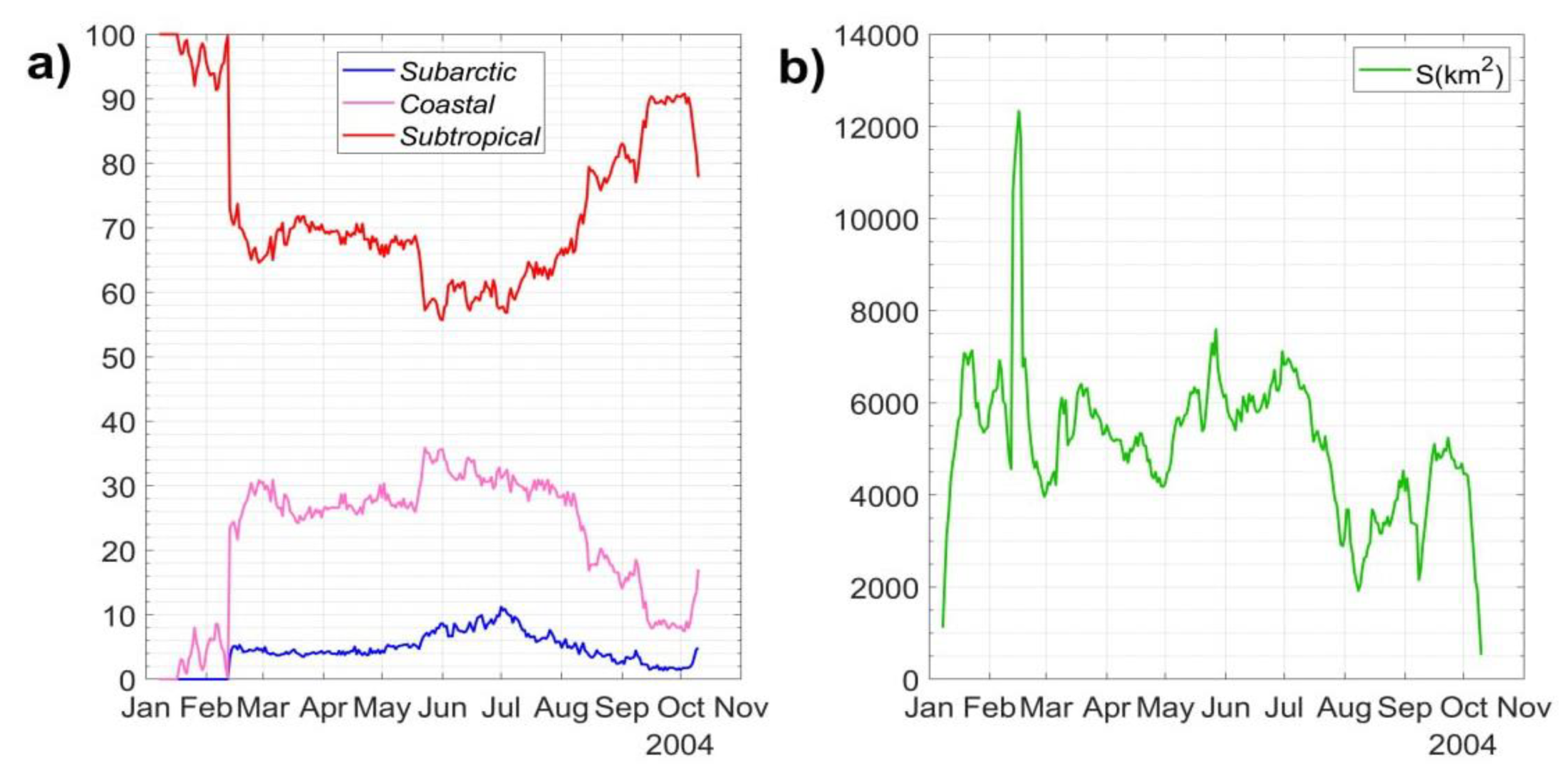
In Figure 11a we plot the percentage of subtropical, subarctic and coastal waters in the eddy core during its lifetime that was calculated by dividing , and by the current value of the area under the vortex contour. During the entire lifetime of the eddy, the surface core has been filled mainly with the subtropical water originated in the southern flank of the Subpolar Front. It is consistent with the origin maps in Figure 6, 7, 8 and 9 which show the subtropical water by red color. The episodes with cardinal changes of the percentage of water of different origin in Figure 11 can be compared with the Lagrangian maps on the same dates. An entrainment of the ‘rose’ coastal water begun from February 9. That is reflected in Figure 11a as a rapid increase of portion of coastal water in the vortex core by February 13 due to the decline in the content of subtropical water. Starting from this date, a small amount of subarctic water appears in the core for the first time. The coastal water made up a significant portion of the surface core water until the middle of August (see Figure 10a and the T-map in Figure 9b, where this water is shown in grey). An entrainment of the coastal water occurred also in the middle of May (see Figure 10 and O-maps and SST images in Figure 9), when the eddy was sampled. The final decrease of the content of the subtropical water occurred in the end of life of the eddy (see Figure 11a and the T-map in Figure 10c). As to subarctic water, its amount in the surface core was practically the same from February 13 and by the eventual decay.
The area under the characteristic eddy contour, delineating the surface core, rapidly increased after the formation of the eddy reached approximately 100 km in size by the middle of January. The maximum size of ~120 km was recorded by the middle of February after an entrainment of a large amount of subtropical and coastal waters. Just after that, the eddy destabilized and split into two parts. The erosion of the eddy begun in the beginning of July when it decreased in size from 100 km to 50 km for the month. The eventual decay started in the beginning of October and finished on October 10 (see Figure 10d).
5. Discussion
We used the Lagrangian approach to study the evolution of an ACE in the northwestern JS. On the one hand, this eddy was formed in the region near the Subpolar Front where mesoscale eddies regularly appear and circulated. On the other hand, it was an exceptional long-lived eddy observed with Lagrangian data over 9 months. The eddy was a strong dynamic feature with the diameter reaching 120 km and extended vertically to the bottom that was sampled in details with CTD observations.
We have demonstrated a multilayer structure of this eddy based on ship observations. The eddy had a core of warm and low salinity water between 250 and 400 m which is typical for the eddies observed in the northwestern JS earlier [15]. However, we found other anomalies in its structure which have not observed before including a core of warm and relatively high salinity water between 30 and 230 m, that are slightly warmer and saline as compared to the surroundings, and surface water above the seasonal picnocline. These anomalies in a vertical composition of different water masses in the eddy could be explained by the peculiarities of its evolution.
Using Lagrangian approach, we have traced the eddy evolution over 9 months since January through October 2004. Based on daily-computed L- maps and maps of water origin and water ‘age’ we found a few events of entrainment of surrounding water by the eddy, splitting and merger with neighbor eddies. These events were confirmed by satellite infrared images.
Our analysis demonstrated that an entrainment of subtropical water from the south into the eddy dominated during the whole period of its evolution. It was especially strong in the beginning and in the end of the eddy life cycle, in January and in October. Just after formation and isolation of the eddy from the flow of subtropical water, an entrainment of coastal water surrounding the eddy has increased. Subarctic water from the north was also observed to be entrained into the eddy, however its volume was around ten times lower as compared to that of subtropical water. Large entrainment of surrounding water into the eddy in February caused its rapid enlargement and splitting into two eddies later in this month. Entrainment of surface water from the south, from the area of the Subpolar Front just prior to the ship observation was responsible for formation of surface warm water in the upper 0–30 m observed in the middle of May (WI at Figure 5a).
It is however difficult to explain the origin of higher salinity water in the upper core (HS1 at Figure 5a) and the origin of lower salinity core (LS at Figure 5a). The first water mass could be formed during the process of formation of the eddy in January (Figure 6c and e). The second one could be the result of entrainment and subduction of low salinity intermediate water from the north. It is difficult to judge on the subsurface entrainment and subduction processes using Lagrangian approach based on the satellite altimetry.
Because the simulation results are based eventually on the AVISO velocity field which is imperfect by many reasons, we need to discuss the adequacy of our Lagrangian results in representing reality. First of all, we compared these results, when possible, with observation data and infrared images. The second evidence of the reliability of the results obtained is more sophisticated. The altimetric velocity field in active dynamical areas is, in principle, chaotic (turbulent). Regarding the simulation of particle’s trajectories, it is impossible to obtain ‘true’ trajectories in a chaotic and imperfect velocity field. Even if it would be absolutely perfect, it is impossible to do this because of the exponential sensitivity of output results on small variations in initial conditions and parameters in the real ocean. It is known [27] that the distance between initially closed by particles grows exponentially (on average) with time in a chaotic velocity field resulting in unpredictability of their positions over a definite time interval. This means that any error in specifying initial particle’s positions grows so quickly that it becomes practically impossible to predict final positions with a reasonable confidence interval.
However, in strongly chaotic systems each numerically computed trajectory stays uniformly close to some ‘true’ trajectory with slightly altered initial position [27]. In other words, a computed trajectory is ‘shadowed’ by a ‘true’ one. By integrating advection equations, we compute not a ‘true’ trajectory but a trajectory that is close to this ‘true’ trajectory, and we do not know which one. Therefore, computation with a large number of particles, allows us to track the real pathways of water even in a chaotic field. Thus, in spite of the impossibility of obtaining a specified ‘true’ trajectory, computed pathways for a large congregation of particles approximate real pathways.
As to simulating the processes inside the eddy core, it should be stressed that a large-scale velocity field is smooth and regular there. It allowed us to identify the eddy center with a good accuracy exceeding the nominal resolution of the geostrophic field. Comparing the coordinates of the eddy center in the sampling sections in Figure 3 (41°09’N and 131°15’E) with the calculation of the eddy center on the days of sampling in Figure 9b (41°08’N and 131°11’E), we may conclude that they coincide with the good accuracy of 9 km.
6. Conclusion
The Lagrangian tools have been applied to study in detail an anticyclonic eddy in the northwestern Japan Sea with a strong dynamic feature that was sampled in the cruise in May 2004. The altimetry-based eddy tracking showed that it lived for nine months with the size reaching 100–120 km. The eddy’s characteristics and vertical structure have been studied based on CTD observational data, Lagrangain analysis and satellite data. The eddy had a multilayer structure with a few cores of relatively uniform water with different temperature and salinity characteristics located in its upper layer and intermediate depth (30–400 m). Origin of these cores were associated with the interaction of the eddy with the surrounding waters and neighbor eddies and fronts that caused entrainment of water inside the eddy.
Inspecting daily-computed L- maps and maps of water origin and ‘age’, we documented formation of this eddy, splitting, merger, entrainment and detrainment of water, erosion and eventual decay. All these events have been confirmed by infrared satellite images. A new Lagrangian method has been applied to calculate day by day the percentage of coastal waters and waters of subtropical and subarctic origin inside the eddy core. It has been found that during the evolution the surface core has been filled mainly with the subtropical water originated in the southern flank of the Subpolar Front. The episodes with cardinal changes of ratio of different water types have been recorded and verified with the help of Lagrangian maps.
Author Contributions
M.V.B. computed and analyzed Lagrangian maps, S.Y.L. provided and processed satellite images, V.B.L. eddy sampling and writing the text, S.V.P. designed the research and wrote the paper, A.A.U. developed the codes to track eddies. All authors have read and agreed to the published version of the manuscript.
Funding
The work of MB, SP and AU was supported by the State Task No. 121021700341-2 at the Pacific Oceanological Institute. SL and VL were supported by the State Task No. 121021700346-7.
Data Availability Statement
The data are available upon request.
Acknowledgments
The authors acknowledge research team and the crew of R/V Akademik M.A. Lavrentyev (cruise No.33) and our colleagues at Seoul National University and especially Profs. K. Kim, K.R. Kim and Dr. D.J Kang who contributed a partial fund for this cruise through the Korean CREAMS program.
Conflicts of Interest
The authors declare no conflict of interest.
References
- Park, K.-A.; Chung, J.Y.; Kim, K. Sea surface temperature fronts in the East (Japan) Sea and temporal variations, Geophys. Res. Lett., 2004, 31, L07304. [Google Scholar] [CrossRef]
- Talley, L.D.; Min, D.-H.; Lobanov, V.B.; Luchin, V.; Ponomarev, V.; Salyuk, A.; Shcherbina, A.; Tishchenko, P.; Zhabin, I. Japan/East Sea Water Masses and Their Relation to the Sea’s Circulation. J. Oceanogr., 2006, 19, 32–49. [Google Scholar] [CrossRef]
- Yoshikawa, Y.; Lee, C.M.; Thomas, L.N. The Subpolar Front of the Japan/East Sea. Part III: Competing Roles of Frontal Dynamics and Atmospheric Forcing in Driving Ageostrophic Vertical Circulation and Subduction. J. Phys. Oceanogr., 2012, 42, 991–101. [Google Scholar] [CrossRef]
- Wagawa, T.; Kawaguchi, Y.; Igeta, Y.; Honda, N.; Okunishi, T.; Yabe, I. Observations of oceanic fronts and water-mass properties in the central Japan Sea: Repeated surveys from an underwater glider. J. Mar. Syst., 2020, 201, 103242. [Google Scholar] [CrossRef]
- Chang, K.-I.; Teague, W.J.; Lyu, S.J.; Perkins, H.T.; Lee, D.-K.; Watts, D.R.; Kim, Y.-B.; Mitchell, D.A.; Lee, C.M.; Kim, K. Circulation and currents in the southwestern East/Japan Sea: Overview and review. Prog. Oceanogr., 2004, 61, 105–156. [Google Scholar] [CrossRef]
- Yoon, J.H.; Kim, Y.J. Review on the seasonal variation of the surface circulation in the Japan/East Sea. J. Mar. Syst., 2009, 78, 226–236. [Google Scholar] [CrossRef]
- Lee, D.-K.; Niiler, P.P. The energetic surface circulation patterns of the Japan/East Sea. Deep Sea Res. Part II., 2005, 52, 1547–1563. [Google Scholar] [CrossRef]
- Lee, D.-K.; Niiler, P. Eddies in the southwestern East/Japan Sea. Deep Sea Res. Part I, 2010, 57, 1233–1242. [Google Scholar] [CrossRef]
- Sugimoto, T.; Tameishi, H. Warm core rings, streamers and their role in the fishing ground formation around Japan. Deep Sea Res. Part I Oceanogr. Res. Pap. 1992; 183–201. [Google Scholar] [CrossRef]
- Ginzburg, A.I.; Kostyanoi, A.G.; Ostrovskiy, A.G. Surface circulation of the Japan Sea (satellite information and drifting buoys data). Issledovanie Zemli iz Kosmosa (Russian J. Remote Sens), 1998; 66–83. [Google Scholar]
- Danchenkov, M.A.; Lobanov, V.B.; Nikitin, A.A. Mesoscale eddies in the Japan Sea, their role in circulation and heat transport. Proc. CREAMS’97 Int. Symp., Fukuoka, Japan, 1997; 81–84. [Google Scholar]
- Lobanov, V.B.; Danchenkov, M.A.; Nikitin, A.A. On the role of mesoscale eddies in the Japan Sea water mass transport and modification. J. Oceanogr., 1998, 11, 46. [Google Scholar]
- Takematsu, M.; Ostrovski, A.G.; Nagano, Z. Observations of eddies in the Japan basin interior. J. Oceanogr., 1999, 55, 237–246. [Google Scholar] [CrossRef]
- Lobanov, V.B.; Ponomarev, V.I.; Tishchenko, P.Y.; Talley, L.; Mosyagina, S.; Sagalaev, S.G.; Salyuk, A.N.; Sosnin, V. Evolution of the anticyclonic eddies in the northwestern Japan/East Sea. In: Proceedings of the 11th PAMS/JECSS Workshop, April 11–13, Cheju, Korea, 2001, 37–40.
- Lobanov, V.B.; Ponomarev, V.I.; Salyuk, A.N.; Tishchenko, P.Y.; Talley, L.D. Structure and dynamics of synoptic scale eddies in the northern Japan Sea. Far Eastern Seas of Russia, Ed. V.A. Akulichev. V. 1., Oceanographic Research. Nauka: Moscow. 2007. pp. 450–473.
- Nikitin, A.A.; Lobanov, V.B.; Danchenkov, M.A. Possible ways of warm subtropical water transport into the area of Far Eastern Marine Preserve. Izvestiya TINRO, 2002, 131, 41–53. [Google Scholar]
- Prants, S.V.; Ponomarev, V.I.; Budyansky, M.V.; Uleysky, M.Yu.; Fayman, P.A. Lagrangian analysis of the vertical structure of eddies simulated in the Japan Basin of the Japan/East Sea. Ocean Model., 2015, 86, 128–140. [Google Scholar] [CrossRef]
- Shin, C.-W. Characteristics of a Warm Eddy Observed in the Ulleung Basin in July 2005. Ocean Polar Res 2009, 31, 283–296. [Google Scholar] [CrossRef]
- Mitchell, D.A.; Teague, W.J.; Wimbush, M.; Watts, D.R.; Sutyrin, G.G. The Dok Cold Eddy, J. Phys. Oceanogr., 2005, 35, 273–288. [Google Scholar] [CrossRef]
- Prants, S.V.; Budyansky, M.V.; Uleysky, M.Yu. Statistical analysis of Lagrangian transport of subtropical waters in the Japan Sea based on AVISO altimetry data. Nonlin. Processes Geophys. 2017a; 24, 89–99. [Google Scholar] [CrossRef]
- Ivankova, V.N.; Samoilova, A.E. New fish species for the USSR waters and an invasion of heat-loving fauna in the north-western part of the Japan Sea. Voprosy Ihtiologii, 1979, 19, 449–550. [Google Scholar]
- Le Vu, B.; Stegner, A.; Arsouze, T. Angular Momentum Eddy Detection and Tracking Algorithm (AMEDA) and its Application to Coastal Eddy Formation. J. Atmos. Ocean. Tech. 7: 35, 2018; 35, 739–762. [Google Scholar] [CrossRef]
- Prants, S.V.; Uleysky, M.Yu.; Budyansky, M.V. Lagrangian Oceanography: Large-scale Transport and Mixing in the Ocean. Physics of Earth and Space Environments. Springer-Verlag: Berlin, Germany, 2017b; pp. 287.
- Ponomarev, V.I.; Fayman, P.A.; Prants, S.V.; Budyansky, M.V.; Uleysky, M.Yu. Simulation of mesoscale circulation in the Tatar Strait of the Japan Sea. Ocean Model., 2018, 126, 43–55. [Google Scholar] [CrossRef]
- Prants, S.V.; Budyansky, M.V.; Uleysky, M.Yu. How eddies gain, retain and release water: the case study of a Hokkaido anticyclone. J. Geophys. Res. Oceans., 2018, 123, 2081–2096. [Google Scholar] [CrossRef]
- Prants, S.V.; Lobanov, V.B.; Budyansky, M.V.; Uleysky, M.Y. Lagrangian analysis of formation, structure, evolution and splitting of anticyclonic Kuril eddies. Deep Sea Res. I., 2016, 109, 61–75. [Google Scholar] [CrossRef]
- Ott, E. Chaos in Dynamical Systems. Cambridge University Press, 2002; pp. 492.
Figure 1.
Fronts and eddies in the Japan Sea based on 10-day mean temperature distribution at 100 m depth for 11–20 May 2004 (JMA data). Schematic location of the Subpolar Front is indicated by the white dashed line (SF). Warm-core anticyclonic eddies are observed to the north of the front (A), over Yamato Rise (YE), in the Ulleung Basin (UE), east off Oki Spur (OE) and at other locations. Location of the studied anticyclonic mesoscale eddy on these dates is indicated as A.
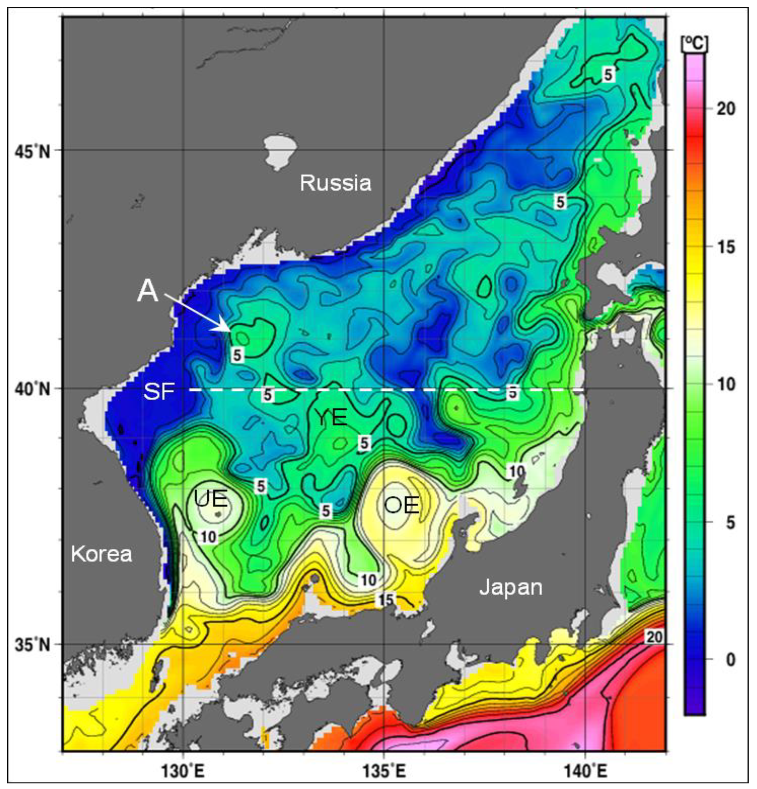
Figure 2.
The occurrence frequency of anticyclones with the lifespan exceeding 30 days in the northwestern Japan Sea in 1993–2021 with the imposed formation (a) and decay (b) sites. The sites of formation and decay of the studied eddy are shown in a) and b) by stars on January 9 and October 10, 2004, respectively.
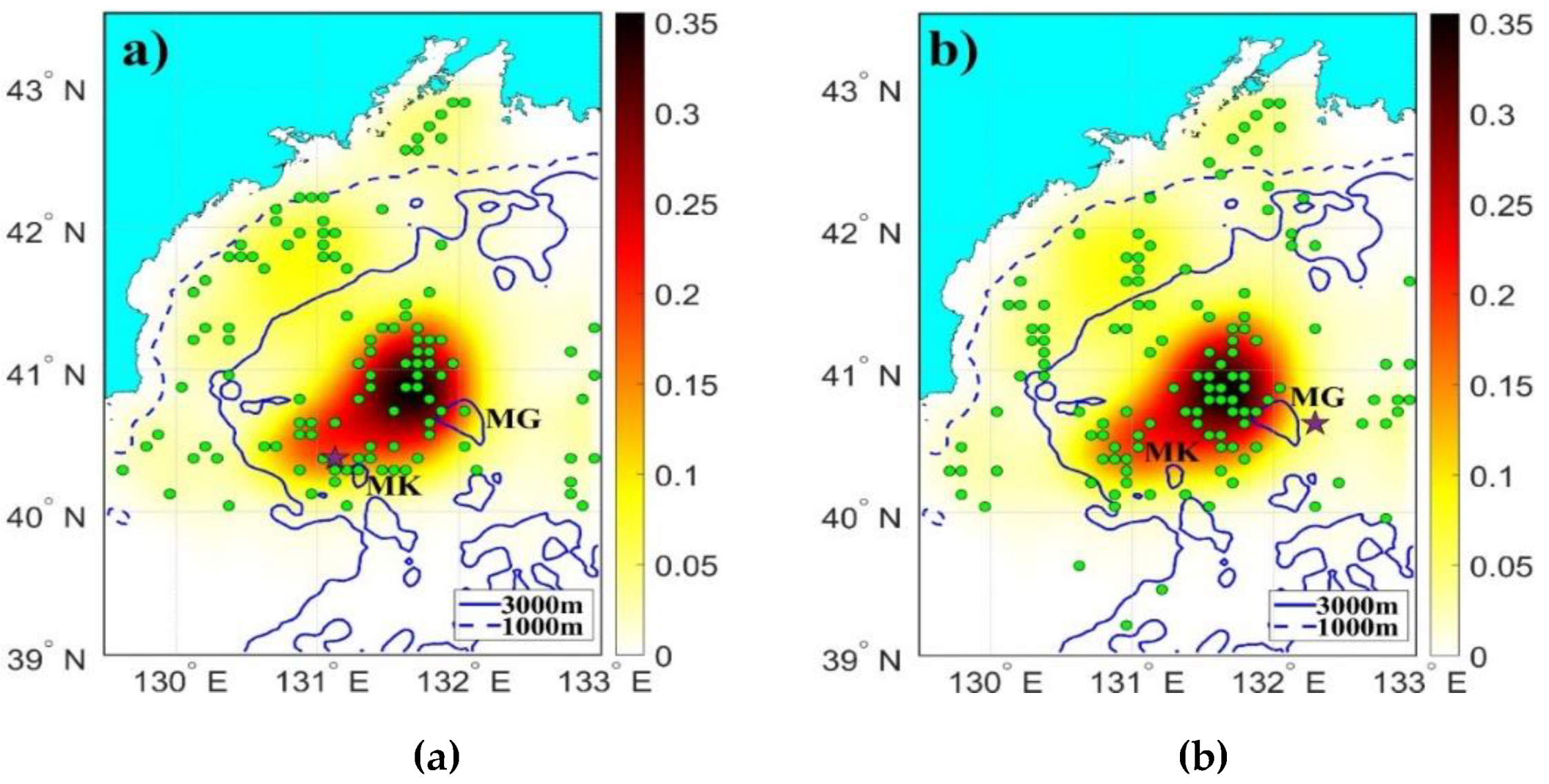
Figure 3.
(a) Temperature and (b) salinity distribution at 300 m based on ship CTD observations in 11–16 May, 2004. Location of the studied eddy A is indicated by the arrow.
Figure 3.
(a) Temperature and (b) salinity distribution at 300 m based on ship CTD observations in 11–16 May, 2004. Location of the studied eddy A is indicated by the arrow.
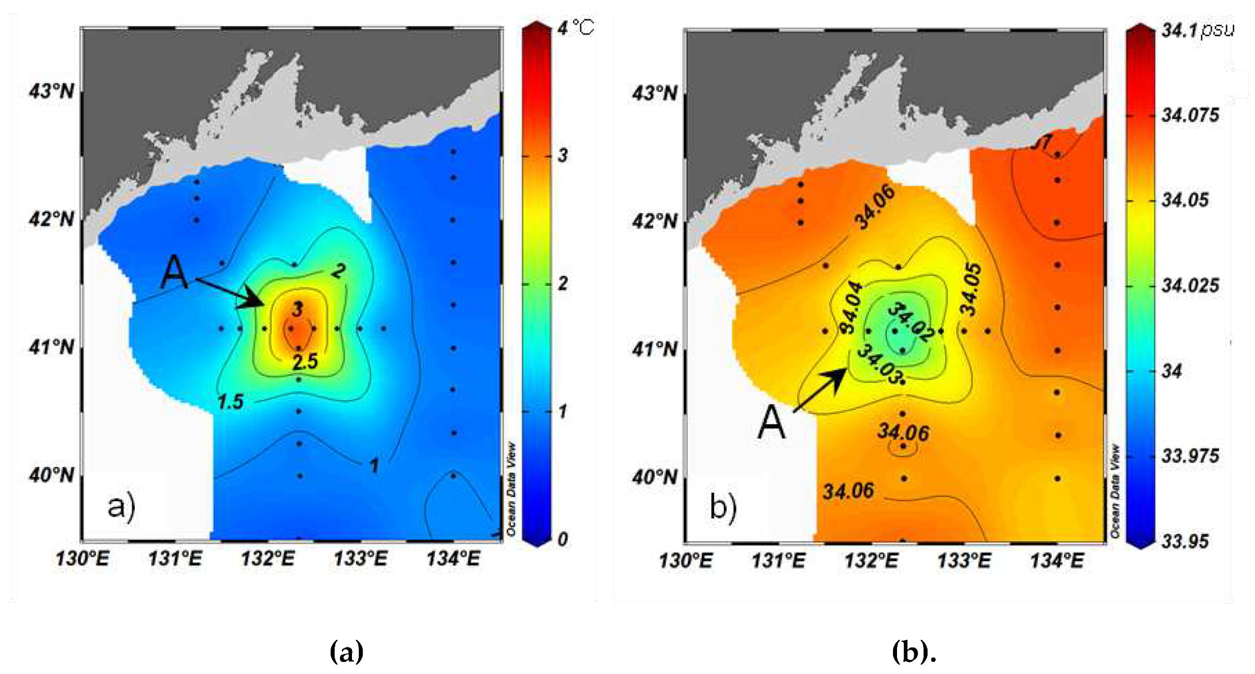
Figure 4.
(a) Dynamic topography of the sea surface relative to 1500 m (dyn m) and (b) vertical distribution of meridional component of geostrophic velocity (cm/c) along the section 41°09’N crossing the eddy A based on the ship CTD observations in 11–16 May, 2004. Red and blue color correspond to northward and southward flows.
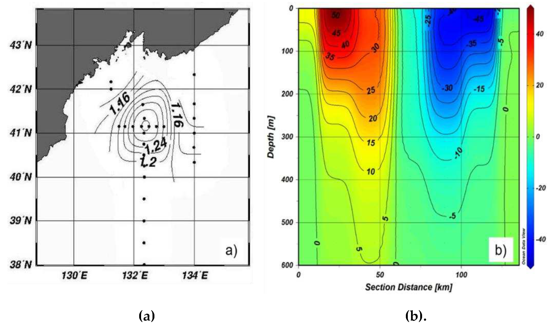
Figure 5.
(a) Temperature (°C) and (b) salinity (psu) distributions along the zonal section (41°09’N) crossing the eddy A based on the CTD observations in 14–16 May, 2004. WI – warm intrusion; UC – vertically uniformed core; HS1 – upper high salinity layer; LS – low salinity core; HS2 – lower high salinity layer.
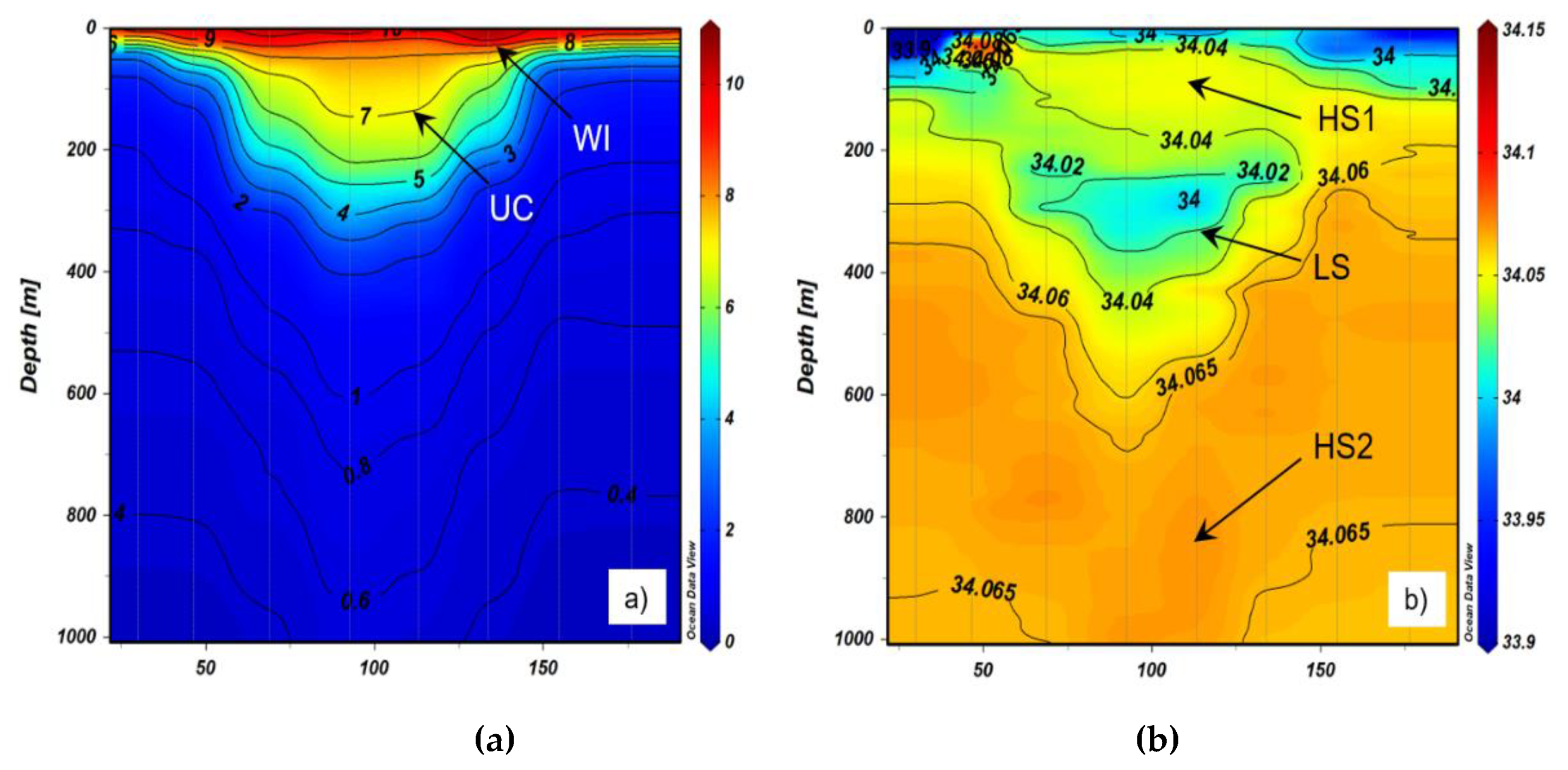
Figure 6.
Backward-in-time Lagrangian maps and SST images in January 2004. (a) and (b) L-maps, (c) and (d) origin maps with imposed AVISO velocity field show the eddy formation. Rose color on the maps codes virtual particles which got into AVISO coastal grid cells prior the dates indicated on the maps. Gradation of the blue color on the L-maps shows the length of the pass covered by the virtual particles for 30 days in the past. Red and blue colors on the origin maps code subtropical and subarctic waters, respectively. The black curves on the O-maps are characteristic contours of the studied eddy (see Sec. 2.1). These contours delineate the core of the eddy at the surface. (e) and (f) SST images on the same dates as in Lagrangian maps (white color means cloudiness). The up(down) oriented triangles denote elliptic points corresponding to the locations of centers of anticyclones (cyclones). The crosses are hyperbolic points.
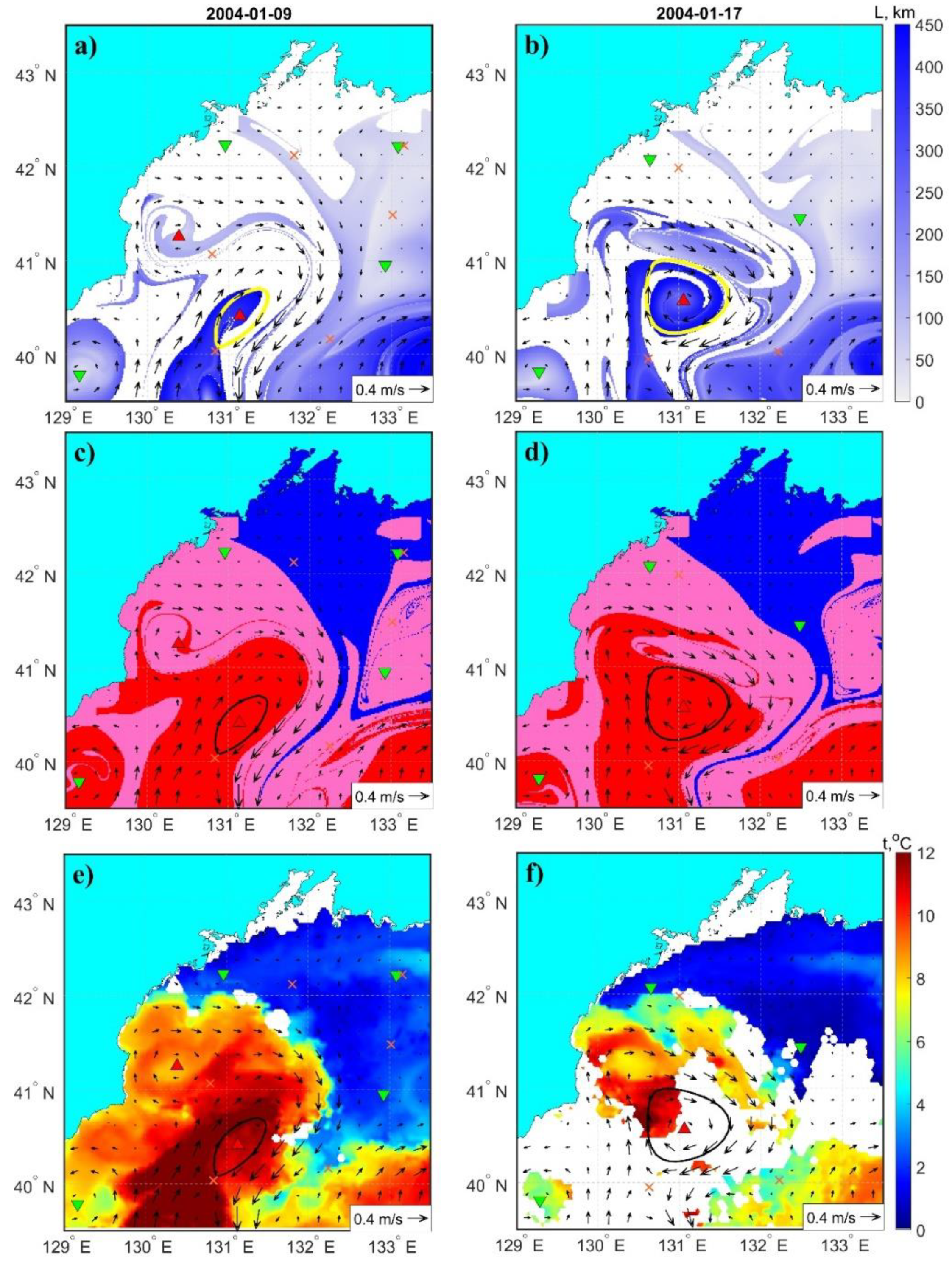
Figure 7.
(a) and (b) L-maps, (c) and (d) SST images with imposed AVISO velocity field show splitting of the eddy A (yellow and black contours) in February.
Figure 7.
(a) and (b) L-maps, (c) and (d) SST images with imposed AVISO velocity field show splitting of the eddy A (yellow and black contours) in February.
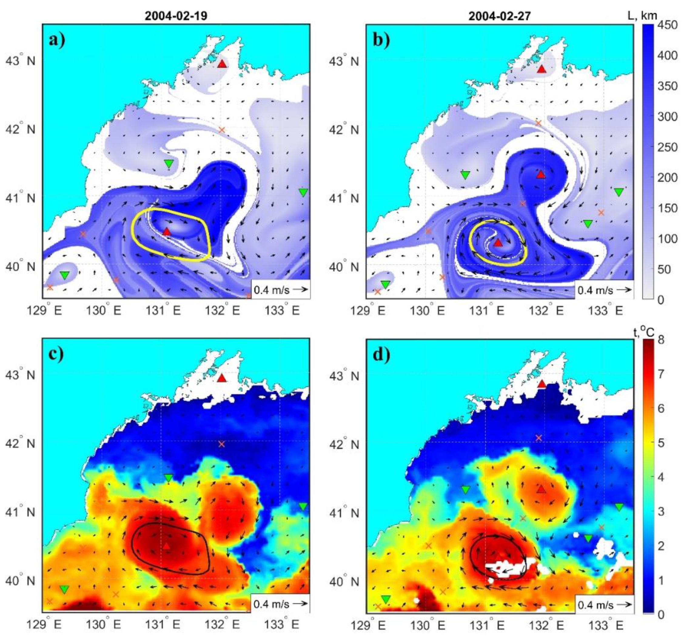
Figure 8.
(a) and (b) L-maps, (c) and (d) origin maps, (e) and (f) SST images with imposed AVISO velocity field show interaction of the splitting products, merger of these products on March 5 and entrainment of water by the united eddy.
Figure 8.
(a) and (b) L-maps, (c) and (d) origin maps, (e) and (f) SST images with imposed AVISO velocity field show interaction of the splitting products, merger of these products on March 5 and entrainment of water by the united eddy.
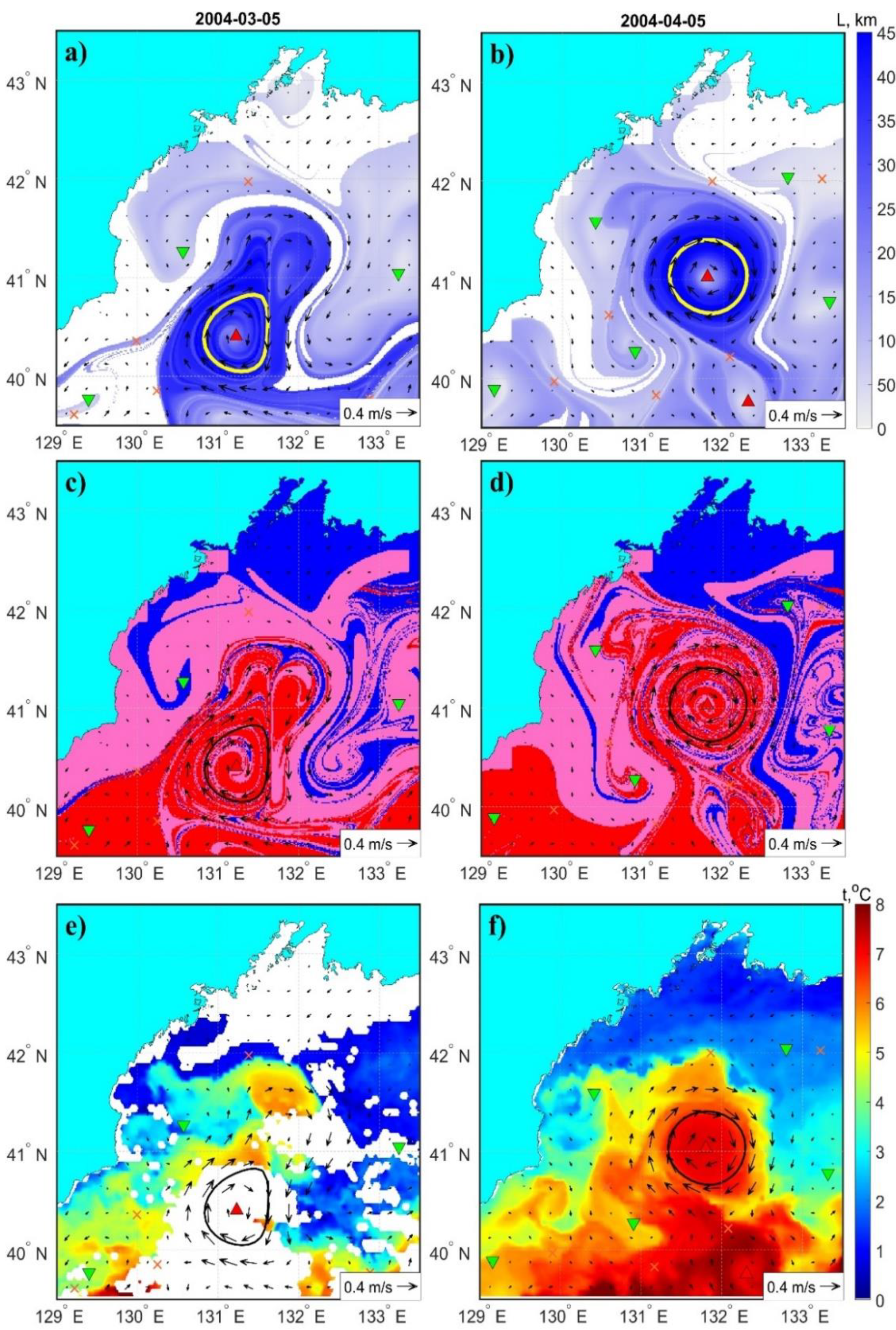
Figure 9.
(a) and (b) L-maps, (c) and (d) origin maps, (e) and (f) SST images with imposed AVISO velocity field show interaction of the splitting products, merger of these products on March 5 and entrainment of water by the united eddy.
Figure 9.
(a) and (b) L-maps, (c) and (d) origin maps, (e) and (f) SST images with imposed AVISO velocity field show interaction of the splitting products, merger of these products on March 5 and entrainment of water by the united eddy.
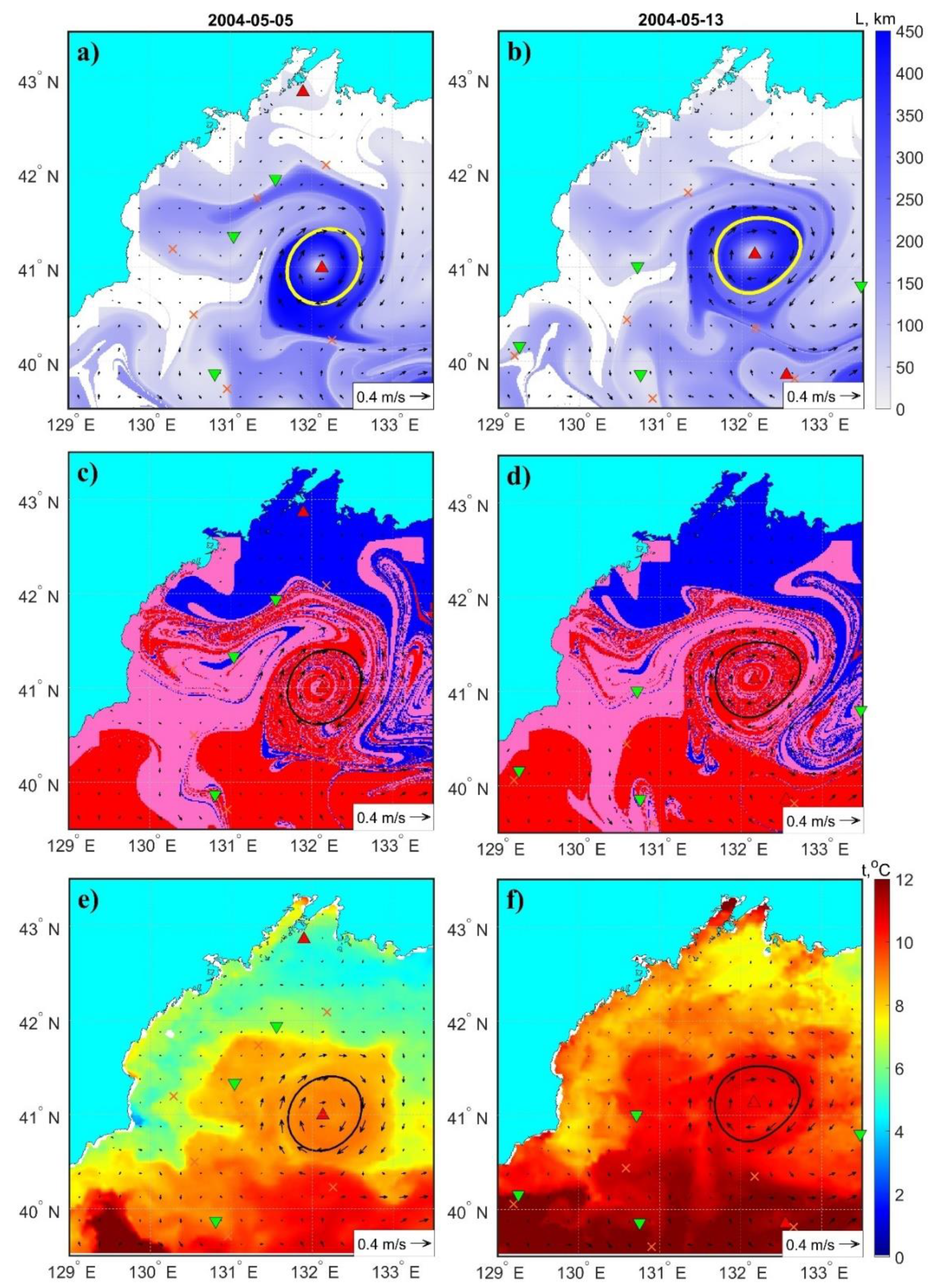
Figure 10.
The water-age T-maps show how ‘old’ is the water inside the studied eddy shown by the yellow contour. Three events in its biography are shown: (a) sampling on May 13, when the eddy had a maximum lateral size, (b) interaction of the weakened eddy with an anticyclone of the Subpolar Front on August 17 and (c) eventual decay on October 10. The legend of colors: nuances of the grey color represent the ‘age’ of subtropical water, green and rose colors represent the ‘age’ of coastal water, the white area to the north of eddy is covered by subarctic water. The blue areas are the AVISO coastal cells.
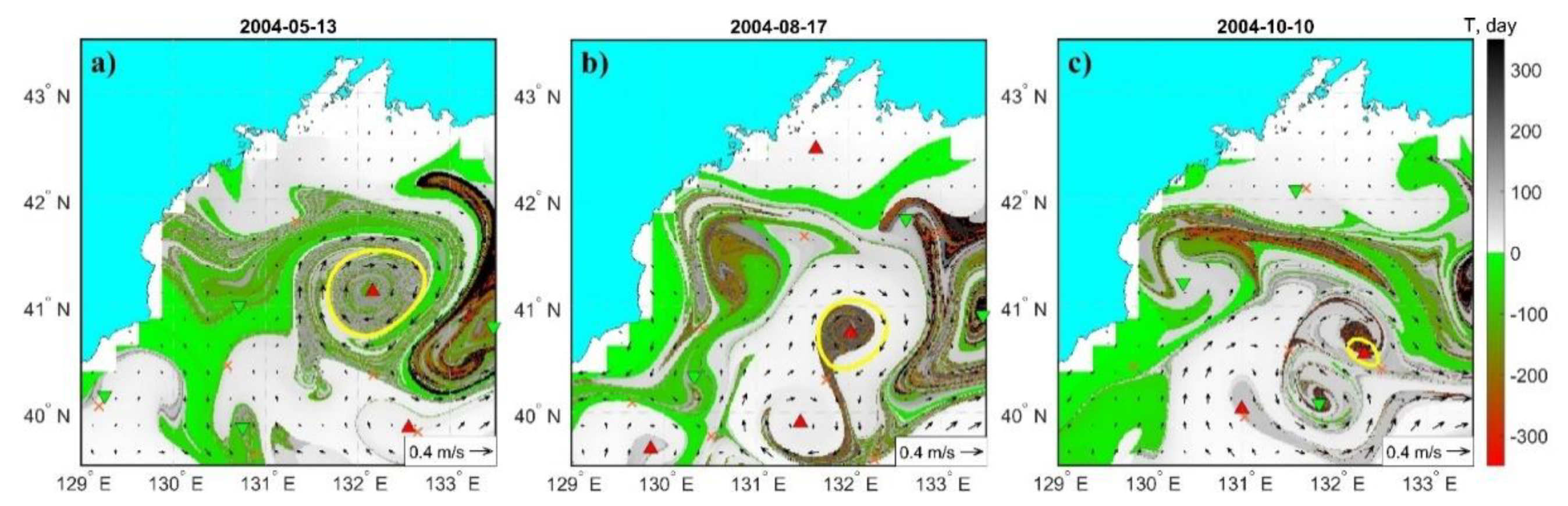
Figure 11.
(a) The percentage of subtropical (red), subarctic (blue) and coastal (rose) waters inside the surface core during the lifetime of the eddy. (b) The area of the surface core of the eddy during its lifetime.
Figure 11.
(a) The percentage of subtropical (red), subarctic (blue) and coastal (rose) waters inside the surface core during the lifetime of the eddy. (b) The area of the surface core of the eddy during its lifetime.
Disclaimer/Publisher’s Note: The statements, opinions and data contained in all publications are solely those of the individual author(s) and contributor(s) and not of MDPI and/or the editor(s). MDPI and/or the editor(s) disclaim responsibility for any injury to people or property resulting from any ideas, methods, instructions or products referred to in the content. |
© 2023 by the authors. Licensee MDPI, Basel, Switzerland. This article is an open access article distributed under the terms and conditions of the Creative Commons Attribution (CC BY) license (http://creativecommons.org/licenses/by/4.0/).
Copyright: This open access article is published under a Creative Commons CC BY 4.0 license, which permit the free download, distribution, and reuse, provided that the author and preprint are cited in any reuse.


