1. Introduction
Nowadays, statistical techniques are necessary for the analysis of massive volumes of data with a spatial argument; this is the case of environmental sciences, climate, geography, econometrics, medicine, biology, and other applied fields. Thus, high-dimensional data becomes functional data which is then processed and analyzed using functional data analysis (FDA) methods and they will be called functional data with spatial correlation. The theoretical and practical aspects resulting from this new branch of statistics have given rise to beneficial advances in areas with geographic dependence (for recent reviews on the subject, see [1]). Indeed, functional data analysis (FDA) has seen rapid growth in recent years, moving from exploratory and descriptive data analysis to linear models and estimation techniques. This dynamic contributes to theoretical and methodological improvements, as well as to the diversification of fields of application (see, for example, [2–4] and through various recent bibliographic discussions such as [5,6]). One of the major subjects in this field of research is functional regression, which studies the influence of a functional random variable on a scalar variable. Among the typical questions that arise on this subject, we find, in particular semi-parametric functional regression models that they retain the flexibility of parametric regression models and free themselves from the sensitivity to the dimensional effects of the non-parametric approaches. For a complete discussion with a state of the art on semi-parametric modeling by functional regression, we refer the readers to the bibliographical surveys of [7].
In particular, one of the most important semi-parametric functional models is the partially linear regression model introduced by [8], which is called the semi-functional partial linear regression (SPFLR) model, and therefore, many works were carried out to estimate and apply this model. This model is expressed as:
where
Y is the scalar response variable,
is a
p-vector of explanatory variables,
is unknown
p-dimensional parameter vector,
Z is functional explanatory variable,
is an unknown smooth functional operator and
are identically distributed random errors satisfying
and unknown variance
. We generally assume an additional condition of independence of the variable error
with respect to the random vector
. The authors use the classical kernel method (Nadaraya-Watson type weights method) to prove the asymptotic normality of
and the convergence rate of
m. This model was extended to dependent data by [9]. Furthermore, [10] proposed a bootstrap procedure to approximate the distribution of these estimators, while [11] proposes to generalize this model to the case where the linear component is also functional. More recently, [12] studied different bootstrapping procedures for this model under dependency structures. Additionally, a procedure for testing linearity in partially linear functional models is proposed in [13]. Other approaches have been proposed to estimate SPFLR model parameters; we cite, for example, the local linear approach used by [14], the robust procedures considered by [15], the
k nearest neighbors (
kNN) procedure used by [16] and Bayesian approaches proposed by [17]. For recent advances, we can consult the bibliographic reviews in [6,18].
Furthermore, only a few research works have paid attention to estimation in the semi-functional partial linear regression model for spatially dependent observations. We cite the work of [19] on the autoregressive semi-functional linear regression (SAR) model, which proposed an estimator based on the method of quasi-maximum likelihood and local linear estimation while [20] obtained the asymptotic normality of the parametric component as well as the convergence in probability with the rate of the nonparametric component. The complete analysis of the data is the subject of all the works listed. On the other hand, in many applications, this is unfortunately not the case, and we are faced with missing data. There are several common causes of missed responses, including faulty equipment, sample contamination, manufacturing defects, clinical study dropouts, climatic circumstances, inaccurate data entry, and more. On this subject, filling in missing data and the uncertainty linked to such imputation has been the subject of in-depth studies in the multivariate case (see, for example, [21,22]). However, little research on nonparametric functional regression with missing data has been done. The first work was carried out by [23] to estimate the mean of a scalar response using an i.i.d. functional sample. The functional regressor is fully observed, with some responses missing at random (MAR). They generalize the result obtained in [24] in the multivariate case. While [25] took into account the estimation of the regression function and established these asymptotic properties under the condition of stationarity and ergodicity with MAR response. On the other hand, [26] used the k nearest neighbors method (k-NN) combined with the local linear method to estimate the regression function with a low number of randomly missing values repones (MAR). For semi-parametric partially linear multivariate models with randomly missing responses, we can cite the work of [27,28] while [29] is the first to study the SFPLR model for i.i.d data with a MAR response, and their results generalize those obtained in [27].
However, the handling of missing data for spatial data is very weak. We cite the work of [30] in the multivariate case to estimate the regression function with the kernel method. The performance of the estimator obtained is compared with the K nearest neighbors method.[31] considers multiple spatial regression models with missing data using the regression-based imputation method to predict missing values and adds a normally distributed residual term to each predicted value. It restores the loss of variability and biases associated with regression imputation. For functional data, we cite [32], which proposes to study the kernel estimation of the regression function when the data are spatially functional and MAR. They obtain the asymptotic properties of this estimator, notably the probability convergence (with rates) and the asymptotic normality of the estimator under certain weak conditions.
In this study, we propose to study SFPLR models for spatial data with missing responses. Our paper is organized as follows. In
Section 2, the semi functional partial linear model for spatial data is presented with these estimators as well as the notations and hypotheses used in our work. whereas
Section 3 is devoted to the asymptotic results. The proofs of the asymptotic results are postponed in
Section 4. In section 5, a computer study on simulated and real data is carried out to demonstrate that the proposed estimators allow a nice improvement compared to the usual global approach.
2. The Model and Its Estimators
Let
be the integer lattice points in the
N-dimensional Euclidean space and let
be a measurable strictly stationary spatial process defined over a probability space
and identically distributed as
, where
Y is a response variable that is depend on p-dimensional random vector
in a linear way but is related to another independent functional variable
Z in an indeterminate form by means of an SFPLR model
where
,
,
and
are defined as before such that
and .
We assume that Z is valued in semi-metric space , where the associated semi-metric is denoted by and we denote by such that the topological closed ball. We further assume that the process can be observed in the rectangular region , with a sample size of where . Suppose moreover that, for , approaches infinity at the same rate: for some and we write that if . Remember that the term site is used to designate a point .
The kernel estimators of
and
(see [20]) are defined by:
K denotes a real-valued kernel function and a decreasing sequence of bandwidths which tends to zero as tends to infinity.
In this article, we develop an estimation approach in which the values of the independent variables (
X and
Z) are all observed, however, some observations of the response variable (
Y values) are missing. We recall that we say that
is missing if
does not contain all of the required elements. For this we consider a real random variable denoted
such that
if the value
is known, and
otherwise. Thus, the study will be carried out on an incomplete sample of size n:
It is assumed that the random missing data mechanism satisfies the saving condition
This conditional probability
is generally unknown.
First, we note that
From our assumption,by conditioning on
, it follows that
from where we have
In the following, we define , and we write .
Then, by equations
5 and
6, we can write
Thus, if the functions
and
are known, the least squares estimator of
is given by
However,
and
are generally unknown and they must be estimated for applied
8. Assuming that
and
are smooth functions of
, these can be estimated by using the nonparametric Nadaraya-Watson kernel estimator noted by
and
and expressed by
where
with
K is a real-valued kernel function and
a decreasing sequence of bandwidths which tends to zero as
tends to infinity.
Hence, an estimator of
is given by
where
and .
We then insert
in equation
7 to obtain
3. Notations and Hypotheses
Our main objective is to obtain the asymptotic normality of our estimator under the condition that the process
is strictly stationary, which satisfies the following
-mixing condition (see [33]): there exists a real function
which tends to 0 when
t goes to
∞, such that for finite cardinal subsets ( Card
)
:
where
denotes the Euclidean distance in
,
, for
,the
-fields generated by a random variable
and
is a symmetric positive function nondecreasing in each variable such that:
Moreover, as is often the case in spatial regression, we assume other condition on the function
:
In what follows, in order to simplify the writings, we introduce the following notations:
and we need the following assumptions which are necessary to prove and obtain our results.
(H1): Let the probabilistic joint distribution of and and let the small ball probability.
We suppose that, and , there exist such that,
(H2): The kernel function
is assumed to be differentiable with support in the interval
such that there exist two constants
and
with
(H3): We assume that any function
is smooth i.e there exists
such that for
, we have:
,
(H4) There exists a differentiable nonnegative functions
and
g such that:
(H5) For all
, we have:
(H6) Let and , where is the site spatial and we denote by he site spatial .
i) The matrix is assumed positive definite.
ii) We assume that is an invertible matrix.
(H7): We suppose that:
i) for some
ii) For all
iii) For all .
(H8)
i) Let
and
, with
. We suppose that the function
and
is continuous function near
z, i.e. since
h tends toward 0, we have
ii) Let
, for
.
We suppose that the function V is continuous in some neighborhood of .
(H9) We also suppose that
, is continuous function near
z, i.e,
(H10) There exists
, in such that,
.
Comments on the assumptions
The asymptotic results obtained subsequently are based on Theorem 4.1 [32] (see the proof section). It is, therefore, normal to impose the same hypotheses as in this theorem, as well as to hypotheses (H1)–(H5) and (H7)-H(10) (for comments on these hypotheses, see [32]). The additional hypothesis (H6) is usual in the context of the SFPLR.
4. Theoretical Results
We are now in a position to give our asymptotic results. The first one gives the asymptotic distribution of the estimator for the parametric component of the model ().
Theorem 1.
When the assumptions (H1)-(H10), 11, 12, 13 hold, if additionally the bandwidth parameter and the function satisfies and , when , we have:
The following results give the probability convergence and the asymptotic normality of the estimator of the non-parametric part.
Theorem 2.
Based on hypotheses of the Theorem 1, we have:
Theorem 3.
Under the assumptions of 1, if in addition, , as , we have
where , with , for .
We note that these results obtained extend those which are established in the case of complete data (see [20]).
5. Proof
Throughout the rest of this paper, we set, , for all .
First, we recall the following results (Theorem 4.1 in [32]), which will be used in the demonstrations of our results.
Lemma 1.
Under hypotheses (H1)-(H10), 11, 12, 13, if additionally the bandwidth parameter and the function satisfies and , when tend to ∞, then
Second, we need to state some preliminary results.
We denote by and we define the random variable by
Lemma 2.
Based on hypotheses of the Theorem 1, we have:
Proof:
Before going further, note that
First, we have .
Conditioning on
and using MAR assumption, we have
then,
and
implies
Similarly, conditioning on
and using MAR assumption we have
It follows, by
and
, that:
and by
and
that:
From where, we have
which implies that
and, thus
On other hand, using
,
, we leads to the fact that
For the covariance term
, taking account that
then, by some argument as above, we have
In the following, we introduce the following sets
where
is a real sequence that tends to
as
, which will be specified later, and we note in the following
On one hand, by assumption
, we have:
On the other hand, by Lemma (3.3) in [33] and using the fact that the random variables
are bounded, we have
Consequently, we have
Then, by the condition (
13); if we ask
, we have
So the equations (
21), (
22) and (
23) implies that
The proof concludes from (
18), (
20), (
25) ◾
Using the lemma 2 and the same reasoning as in the proof of Theorem (4.2) in [32], with the same notations, we prove the following result.
Lemma 3.
Under hypotheses (H1)-(H10), if the bandwidth parameter and if the function satisfies and as then, we have
with .
Lemma 4.
For the hypotheses (H1) through (H10), if additionally and , when tend to ∞, then we have:
Proof:
Taking account that
where
Then, by the strong law of large numbers and the MAR assumption, we have that
Second, by the lemma 1 and Cauchy-Schwartz inequality, it is easy to check that
and
So, we conclude the proof of Lemma 4 by using (
29)-(
31).
◾
Proof of Theorem 1 Let us use the following decomposition:
So, by using (
30)-(
31) and the Cauchy-Schwartz inequality, we can see that
Which implies, by using Lemma 4, that
Then, according to the condition
(H6)(ii) and by applying
theorem 6.1.1 in [35] on {
}, we have:
The proof concludes from (
30), (
34), (
35) and Lemma 4.
◾
Proof of Theorem 2.
It suffices to see that
Then, we have
On the other hand, we can write
Then, by the theorem 1,
converge in probability to 0 and according to
(H7), we have
Moreover, by the lemma 1, we have
Thus, from (
37)-(
39) the proof is over.
◾
Proof of Theorem 3.
From
36, we have
Now, by lemma 3, we have
and by the theorem 1, we have
Then, from (
40)-(
41) the proof is over.
◾
6. Computational Study
In this section, we are interested in the behavior of the estimators proposed on samples of finite size, with particular attention to the influence of spatial correlation and the effect of MAR on the efficiency of the estimators. To do that, we conducted simulations based on observations denoted as
with
,
,
, and we generate the SFPLR model with MAR as follows:
where
,
and take the nonparametric operator
m as follows
The curves
were
For simulated the curves
, we take
,
with
,
and
where the function
denotes a stationary Gaussian random field with mean
and covariance function defined by
and
. and the function
D is defined by
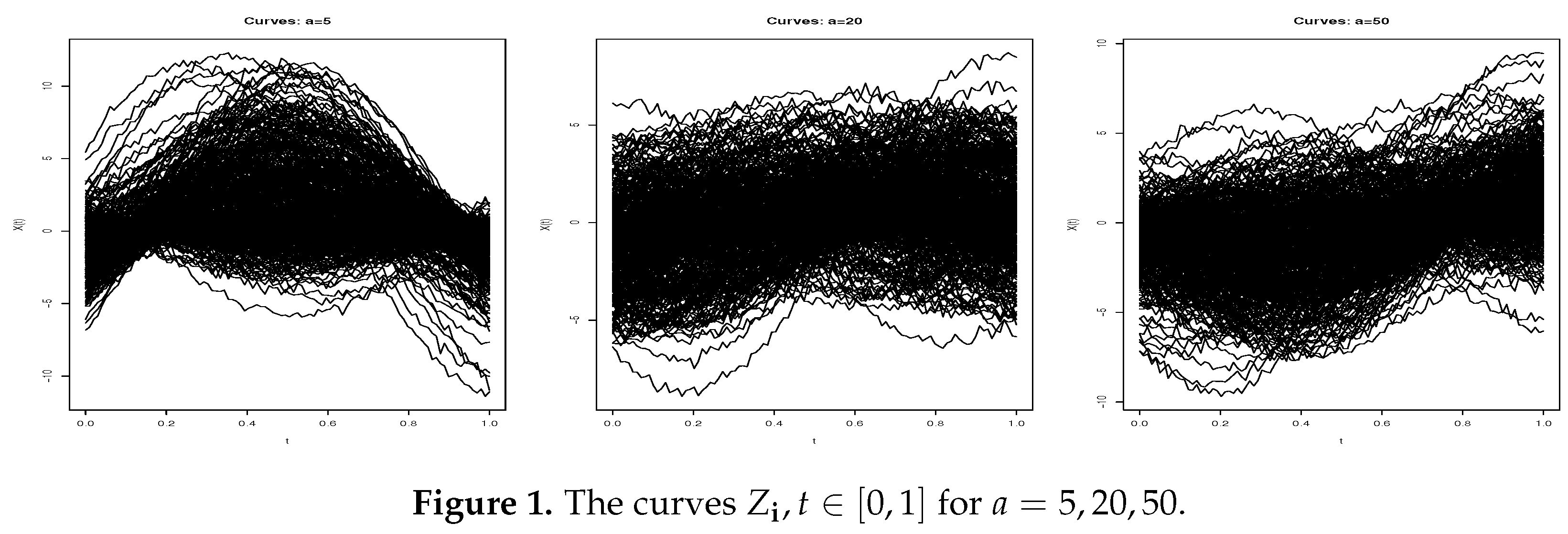
. The curves, following the values of
a, are displayed in
Figure 1. Note that we consider the same curves as in [34] where the function
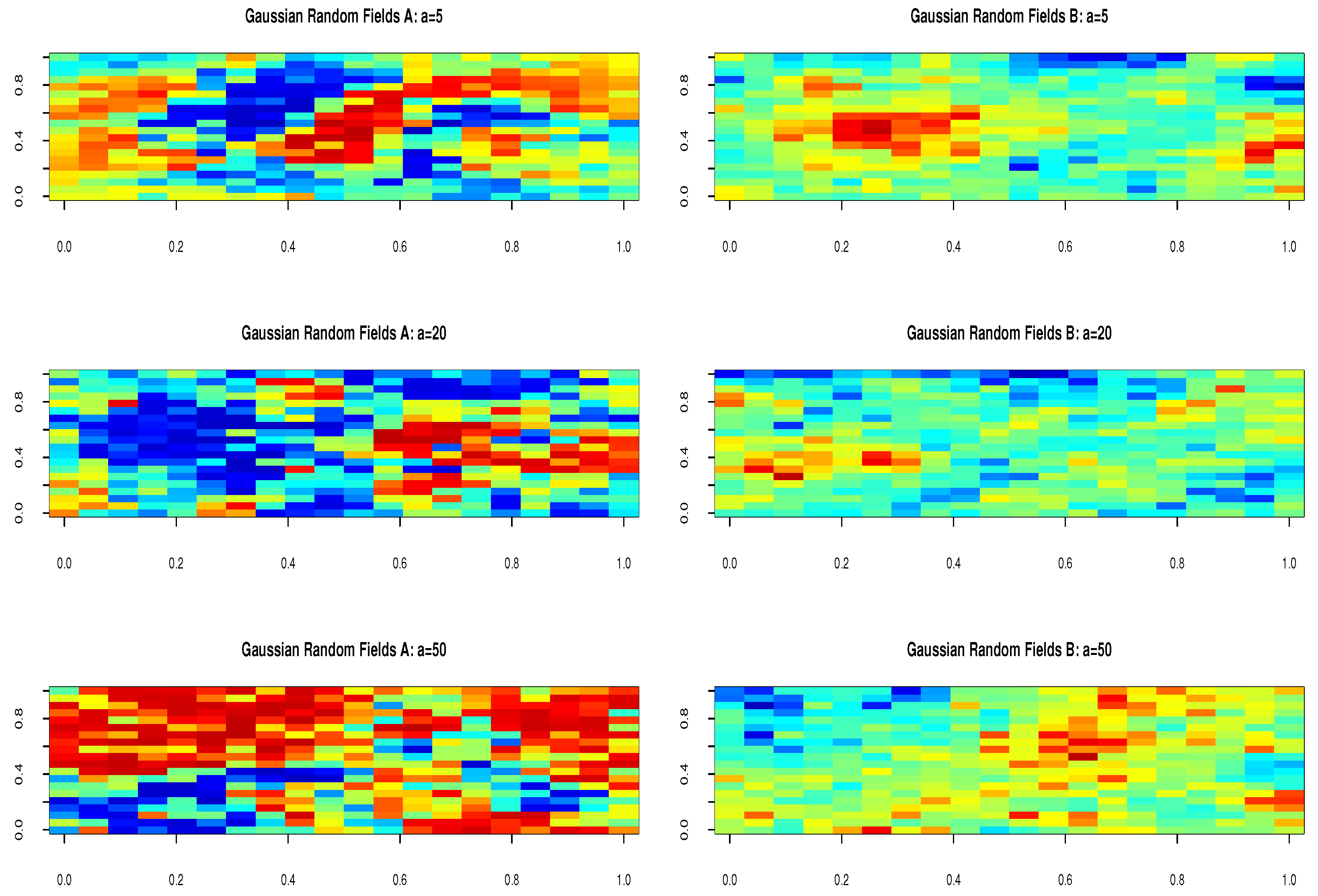
is used to control the spatial mixing condition. Therefore, these observations are a mixture of independent and dependent data points, as illustrated in
Figure 2 (for more details, see [34]). To reduce the level of independence in the data, it is sufficient to decrease the value of
a. For our analysis, we have employed a value of
and
. Moreover, similar to that described in [29], we adopted the following missing data mechanism:
where
for all
and we will take for
the following values:
.
Let’s remember that the degree of dependence between the functional variable Z and the variable is controlled by the parameter and to check the value of , we compute .
In order to calculate our estimators, we use the class of semi-metrics based on the principal component analysis (PCA) metric which is best suited to the treatment of this type of data (discontinuous functional variable). Furthermore, we have chosen the standard kernel function defined as follows: .
The objective of this computer study is to conduct a comparison between our semi-partially linear model with MAR estimator (SFPLRM), semi-partially linear model estimator in the complete case (SFPLRC) (see [20]) and the nonparametric functional model estimator with MAR (FNPM).
Recall that the FNPM model is defined as follows:
and the estimator of operator regression
r (see [32])is given by
For that purpose, we conducted a random split of our data, denoted as
, into two subsets: a test sample
(consisting of data without missing values) and training sample
that they will be used to select the optimal smoothing parameters
, via cross-validation procedures (for more details on the selected tuning parameters, see [4]).
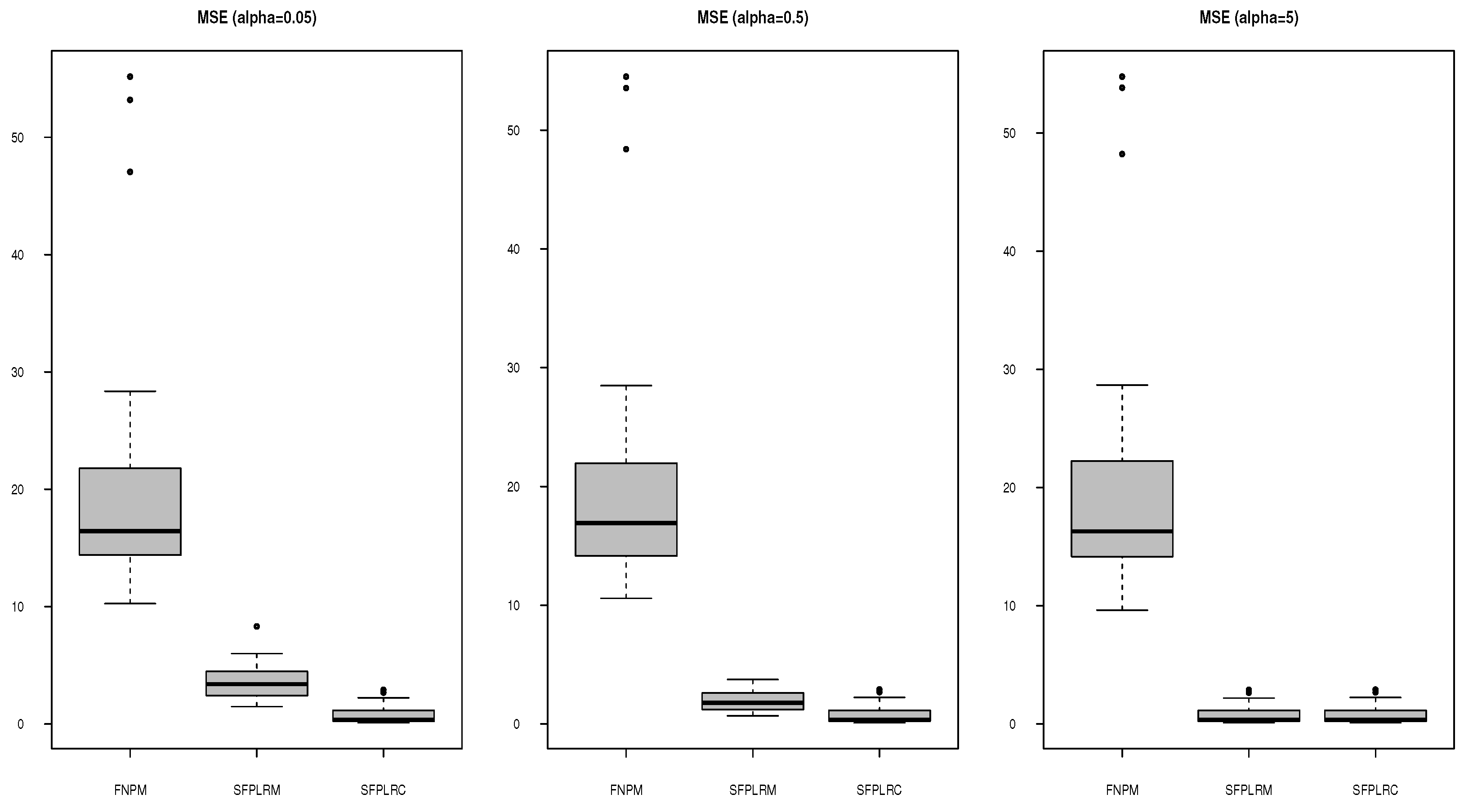
To evaluate the precision of the estimators of the three models (SFPLRM, SFPLRC, and FNPM), we use the square and mean square errors, denoted
:
where
represents the size of the testing sample
. The experiment was replicated
times, which allows us to compute
M values for
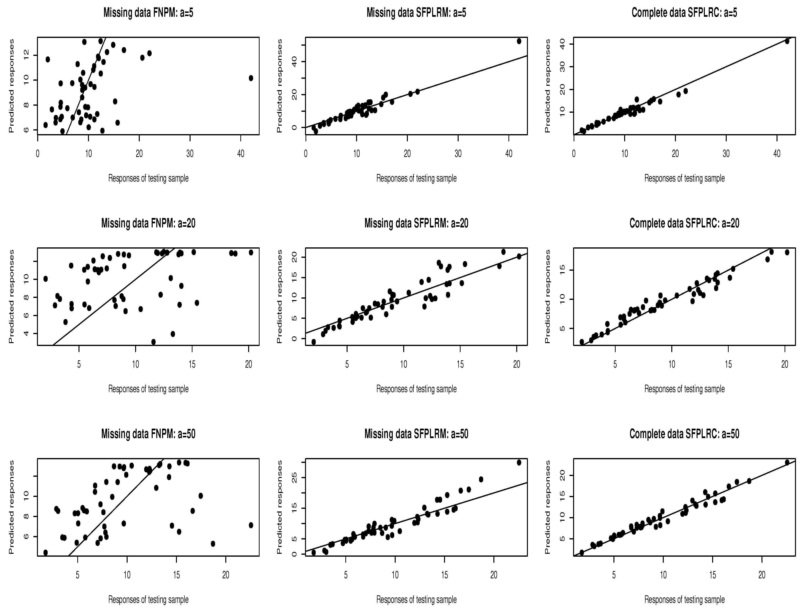
and display their distribution through a boxplot. The results obtained (the prediction values compared with the true values) are presented in
Figure 3 for the three models with different values of
a.
Figure 4 displays boxplots constructed from MSE obtained for the three models.
By
Figure 4, we observe that the SFPLRM estimator shows better prediction effects than the FNPM in comparison to the SFPLRC estimator.
In
Table 1 below, we present the mean squared error (MSE) results for three methods, FNPM, SFPLM, and SFPLR, under various combinations of
,
, and significance level
.
In
Table 1, which presents the mean squared error (
) for FNPM, SFPLRM, and SFPLRC under various conditions defined by combinations of
and
, it becomes evident that the SFPLRM estimator consistently shows superior predictive accuracy when compared to the FNPM estimator across a range of settings. This is notably evident as the
values for the SFPLRM estimator consistently remain lower across the majority of combinations of
and
. Furthermore, a notable observation is that higher values of
(e.g.,
) tend to correspond with lower MSE values, indicating enhanced predictive performance for the SFPLRM estimator. It’s also worth mentioning that as the number of samples (
) increases, the results suggest that the missing at random (MAR) mechanism has little to no discernible effect on the prediction MSE. This observation implies that the SFPLRM estimator maintains consistent performance regardless of the presence of missing data, mainly when dealing with larger sample sizes.
Now, we aim to examine the bias in the estimation of
and its associated Square Error (
), which is defined as:
The results are presented in
Table 2
The results from
Table 2 suggest that the SFPLRM estimator displays good accuracy in estimating the parameters
, with relatively small Square Error values. This implies that the estimator provides reasonably accurate estimates of the true parameters, even in cases with missing data and varying degrees of dependence. The theoretical conclusions of Theorems 3.1 and 3.2 are consistent with such a numerical outcome.
7. Real Data Application
The objective of this part is to compare, on a set of real data consisting of particle pollution indices, the effectiveness of the SFPLR model by our estimators when the data are MAR. The source of these data is the AriaWeb information system, managed by CSI Piemonte and Regione Piemonte, and our analysis is obtained from 34 monitoring sites using gravimetric instruments recorded during the winter season from October 2005 to March 2006 (daily measurements including days). This involves analyzing the levels of pollution, which allowed us to detect higher levels of pollution in the plains closer to urban centers while lower concentrations of this index are observed near the Alps (for more detailed information about the data, we recommend referring to the publication by [36]).
To select the appropriate covariates, a preliminary regression analysis was carried out and the following covariates were selected
: maximum daily mixing height (in meters),
: daily primary aerosol emission rates (in ).
: total daily precipitation (in millimeters),
: the average daily temperature (in Kelvin °).
To implement the theoretical conclusions of the previous section on real data, we will analyze the effectiveness of our estimators built with MAR data in the context of spatial functional prediction which highlights the importance of considering spatial locations. Specifically, we assume that the observations are linked via an SFPLR model (
42), where the response variable is
(in
) (for each
) represents pollution levels, the functional predictor
represents the daily mean temperature curve recorded at the
th station, with its precise location determined by the coordinates
,
and the parametric part are:
, (for 182 days).
if
is observed and
otherwise. Note that our data have some missing values (473 NaN of
for each
and each station, about 7.64% missing data).
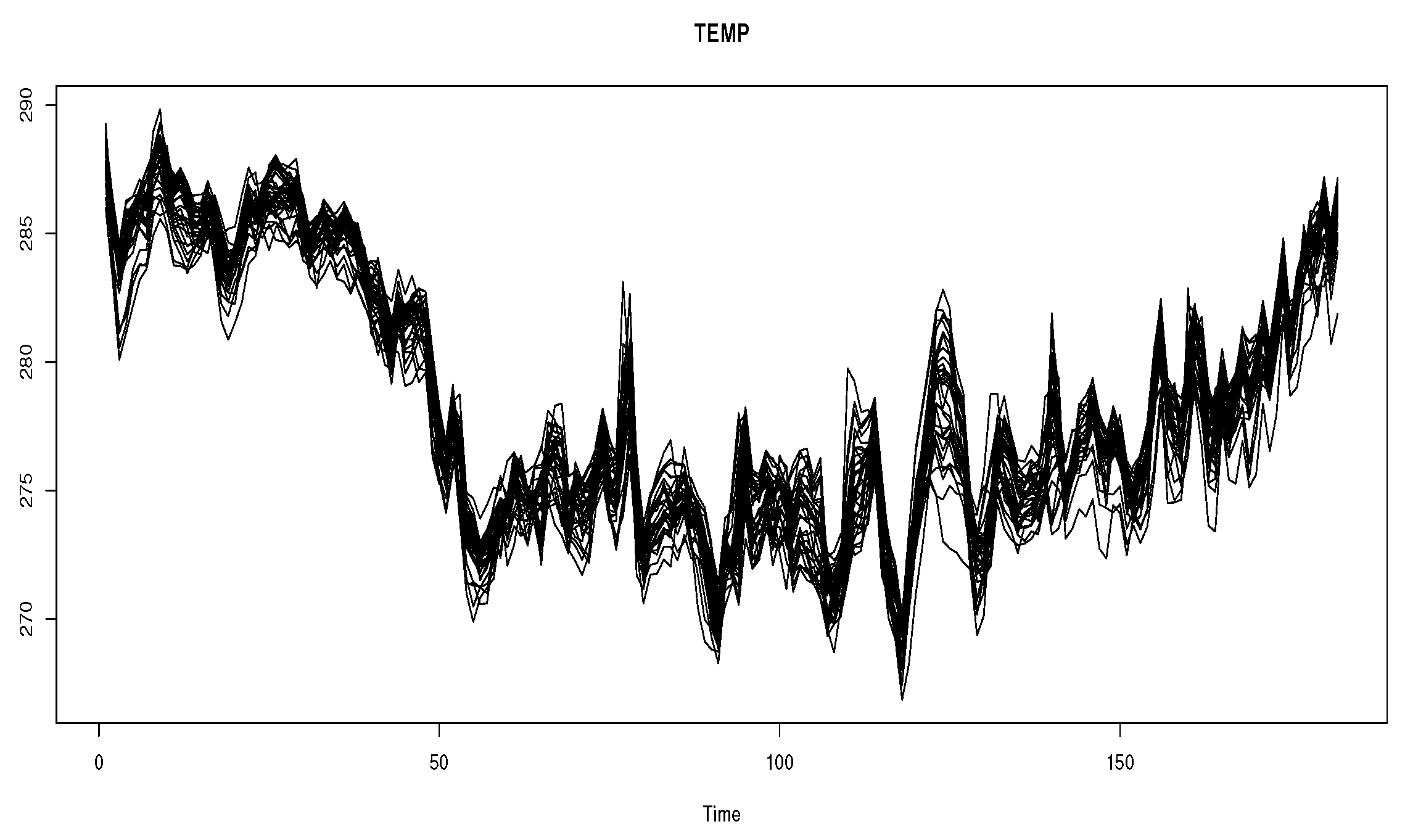
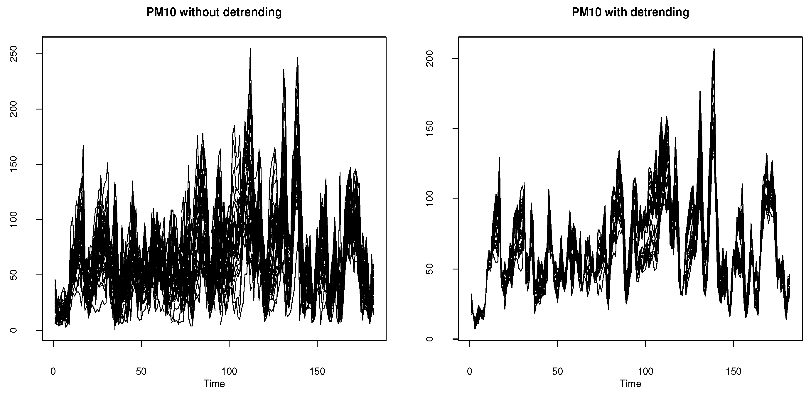
Figure 5 provides the curves of the functional variable
and
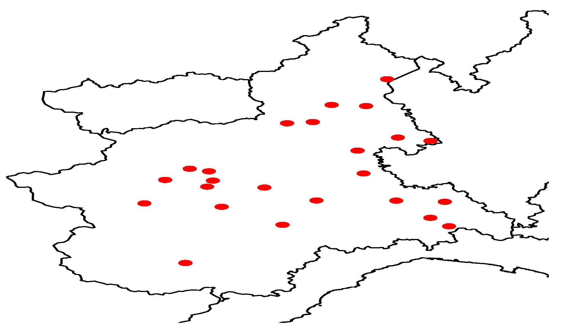
Figure 4 represents the spatial position of the 34 monitoring stations in the Piemonte region (northern Italy)
Figure 5.
Temperature curves Z.
Figure 5.
Temperature curves Z.
Figure 6.
Locations of the stations in Piemonte (northern Italy).
Figure 6.
Locations of the stations in Piemonte (northern Italy).
However, implementing this spatial modeling approach requires preliminary data preparation to validate the stationarity assumption that handles spatial heterogeneity resulting from variations in the effects of space on sampled units. To answer this, we will use an "
detrending step" introduced by [37], which is designed for the multivariate case of the three variables (response, functional, and vectorial explanatory). This algorithm is defined by the following regression.
Thus, instead to the initial observations
, we compute the SFPLRM estimator from the statistics
(see
Figure 7). The latter are obtained by
and
and
are the kernel estimators of the regression functions
and
which are expressed by
where the functions
,
represent kernel functions, while
,
are the bandwidth parameters associated with the actual regression. To illustrate the practical implications of this detrending step on our dataset, we will examine its impact by performing a comparative analysis of the performance of the SFPLRM regression in the two cases, one with detrending and the other without this one.
To conduct this analysis, we employ the same methodology as employed in the simulation example for the selection of the estimator’s parameters. Specifically, we use the quadratic kernel on the interval in combination with the PCA metric and the cross-validation (CV) criterion to determine the smoothing parameter . For the real regressions , , and , we use the npreg routine in the R-package np, with .
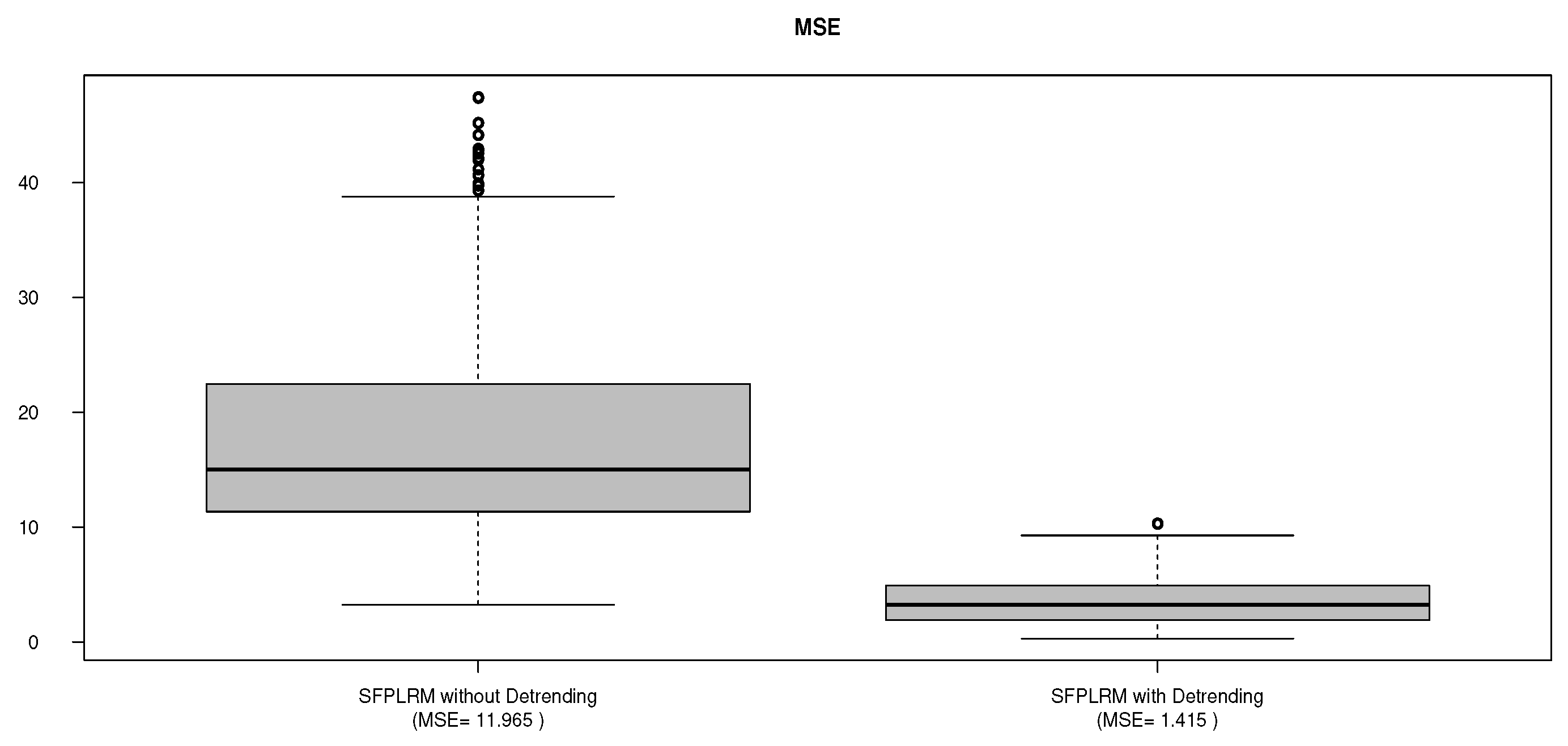
To assess the feasibility of this approach, we randomly split the data sample multiple times (precisely 100 times). The data is divided into two subsets: a learning sample consisting of 24 observations and a test sample containing 10 observations. We then evaluate the significance of the proposed detrending procedure by examining the Mean Squared Error (), as used in the simulation example. This analysis allows us to determine the impact of detrending on the performance of the estimators in practice.
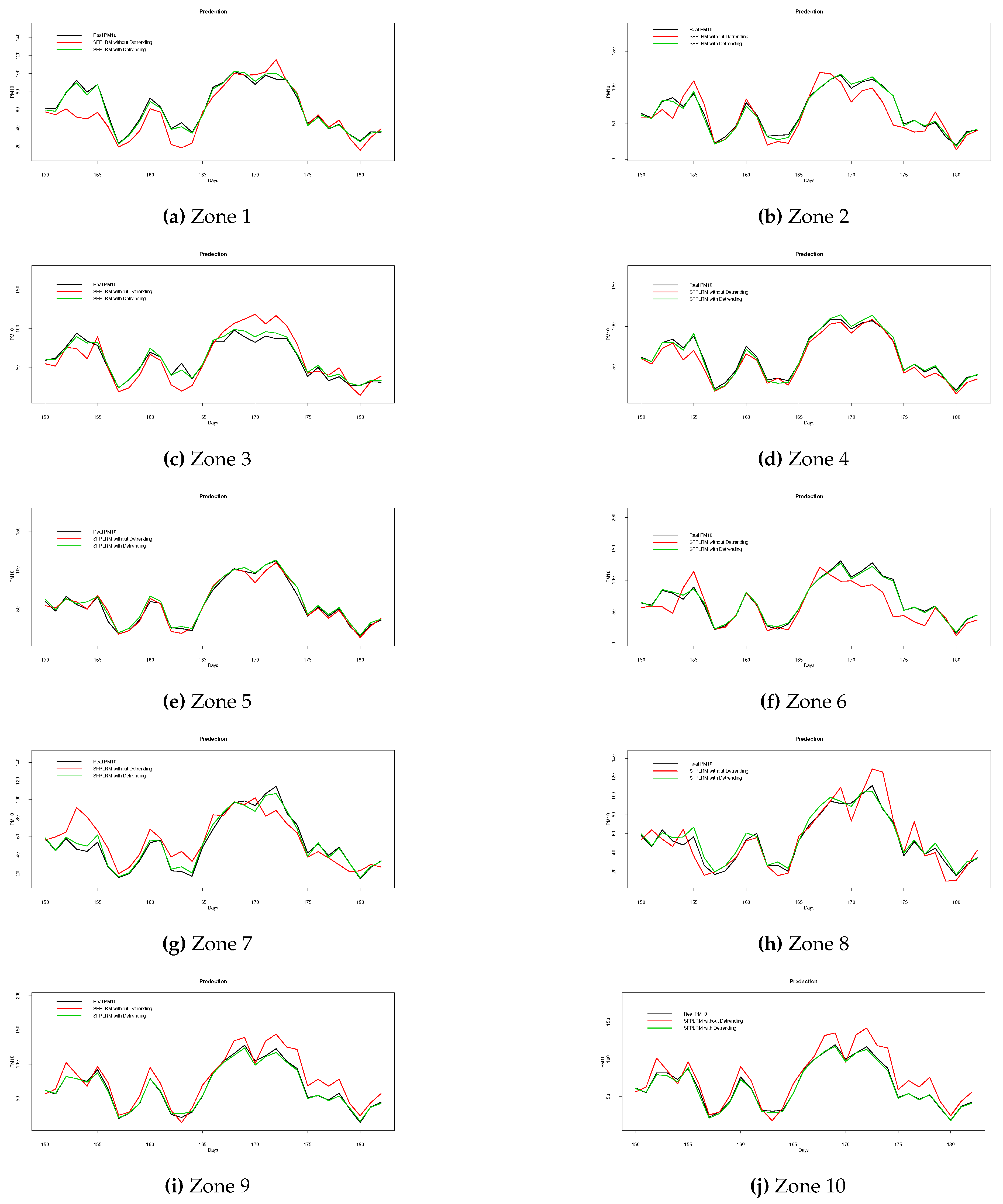
The results in
Figure 8 reveal a significant enhancement in model accuracy with the inclusion of the detrending step. The Mean Squared Error (
) values are substantially reduced when detrending is applied, indicating a clear advantage of this data preprocessing technique. As illustrated in
Figure 9, it becomes apparent that the detrending step consistently outperforms the non-detrending, clearly showcasing its superior capability to accurately capture the underlying functional relationships. These results underscore the pivotal role of detrending in enhancing model performance and underscore the inherent advantages of the SFPLRM estimator in the realm of non-parametric spatial data analysis.
8. Conclusions
This paper addresses the issue of a semi-functional partial linear regression model for spatial data, assuming that the missing responses occur randomly. The construction of the estimator encompasses both the linear and nonparametric components of the model. One crucial aspect of this study involves the demonstration of the asymptotic normality of the best estimators. This is achieved by imposing certain mild constraints and establishing the probability convergence of the nonparametric component. Furthermore, the utilization of both simulated and real data in the analysis serves to underscore the possible viability and adaptability of the model under investigation, along with the estimators derived from it, in the context of predictive tasks. This is achieved through a comparative analysis using a non-parametric estimator. It is essential to highlight that significant emphasis was placed on the absence of a missing mechanism that is missing at random within the domain of functional data statistics.
In the subsequent analysis, it would be intriguing to examine the expansion of our framework into alternative avenues. One such direction is expanding the framework from missing at random (MAR) data to censored data, necessitating the utilization of intricate mathematical techniques.
Author Contributions
The authors contributed approximately equally to this work. All authors have read and agreed to the final version of the manuscript. Formal analysis, Tawfik Benchikh; Validation, Omar Fetitah; Writing – review & editing, Ibrahim M. Almanjahie and Mohammad Kadi Attouch.
Institutional Review Board Statement
Not applicable.
Informed Consent Statement
Not applicable.
Acknowledgments
The authors thank and extend their appreciation to the funder of this work. This work was supported by the Deanship of Scientific Research at King Khalid University through the Large Research Groups Program under grant number R.G.P. 2/406/44.
Conflicts of Interest
The authors declare no conflict of interest.
References
- Mateu, J.; Romano, E. Advances in spatial functional statistics. Stoch Environ Res Risk Assess, 2017, 31, 1–6. [Google Scholar] [CrossRef]
- Ramsay, J.; Silverman, B. Functional Data Analysis, 2nd ed.; Spinger-Verlag: New York, 2005. [Google Scholar]
- Bosq, D.; Blanke, D. Inference and prediction in large dimension; Wiley series in probability and statistics; Wiley: Chichester, 2007. [Google Scholar]
- Ferraty, F.; Vieu, P. Nonparametric functional data analysis. Theory and Practice. Springer Series in Statistics. New York, 2006.
- Aneiros-Pérez, G.; Horová, I.; Hu˜sková, M.; Vieu, P. Editorial for the Special Issue on Functional Data Analysis and Related Fields. J. Multivariate Anal., 2022, 189. [Google Scholar]
- Ling, N.; Vieu, P. Nonparametric modelling for functional data: selected survey and tracks for future. Statistics 2018, 52, 934–949. [Google Scholar] [CrossRef]
- Greven, S.; Scheipl, F. A general framework for functional regression modelling. Statistical Modelling 2017, 17, 1–35. [Google Scholar] [CrossRef]
- Aneiros-Pérez, G.; Vieu, P. Semi-functional partial linear regression. Stat. Probab. Lett. 2006, 76, 1102–1110. [Google Scholar] [CrossRef]
- Aneiros-Pérez, G.; Vieu, P. Nonparametric time series prediction. A semi-functional partial linear modeling. Journal of Multivariate Analysis, 2008, 99, 834–857. [Google Scholar] [CrossRef]
- Aneiros-Pérez, G.; Vieu, P. Automatic estimation procedure in partial linear model with functional data. Stat.Pap. 2011, 52, 751–771. [Google Scholar] [CrossRef]
- H. Lian, Functional partial linear model. J. Nonparametr. Stat. 2011, 23, 115–128. [CrossRef]
- Aneiros Pérez, G.; Raña, R.; Vieu, P.; Vilar, J. Bootstrap in semi-functional partial linear regression under dependence. Test 2018, 27, 659–679. [Google Scholar] [CrossRef]
- Zhao, F.-r.; Zhang, B.-X. Testing Linearity in Functional Partially Linear Models. Acta Mathematicae Applicatae Sinica, English Series 2022. [Google Scholar] [CrossRef]
- Feng, S.; Xue, L. Partially functional linear varying coefficient model. Statistics, 50, 717–732. [Google Scholar] [CrossRef]
- Boente, G.; Vahnovan, A. Robust estimators in semi-functional partial linear regression models. Journal of Multivariate Analysis 2017, 154, 59–87. [Google Scholar] [CrossRef]
- Ling, N.; Aneiros-Pérez, G.; Vieu, P. knn estimation in functional partial linear modeling. Statist. Papers 2020, 61, 423–444. [Google Scholar] [CrossRef]
- Shang, H. Bayesian bandwidth estimation for a semi-functional partial linear regression model with unknown error density. Comput. Stat. 2014, 29, 829–848. [Google Scholar] [CrossRef]
- Ling, N.; Vieu, P. On semiparametric regression in functional data analysis. WIRES Computational Statistics 2020, 12, 20–30. [Google Scholar] [CrossRef]
- Li, Y.; Ying, C. Semi-functional partial linear spatial autoregressive model. Communication in Statistics-Theory and Methods, 2021, 50, 5941–5954. [Google Scholar] [CrossRef]
- Benallou, M.; Attouch, M. K.; Benchikh, T.; Fetitah, O. Asymptotic results of semi-functional partial linear regression estimate under functional spatial dependency. Communications in Statistics-Theory and Methods, 2021, 51, 1–21. [Google Scholar] [CrossRef]
- Graham, J. W. Missing data analysis and design; Springer: New York, NY, USA, 2020. [Google Scholar]
- Little, R. J. A.; Rubin, D. B. Statistical Analysis with Missing Data. 3rd Edition; Wiley Series in Probability and Statistics. 2020.
- Ferraty, F.; Sued, F.; Vieu, P. Mean estimation with data missing at random for functional covariables. Statistics 2013, 47, 688–706. [Google Scholar] [CrossRef]
- Cheng, P.E. Nonparametric estimation of mean functionals with data missing at random. J. Amer. Statist. Assoc. 1994, 89, 81–87. [Google Scholar] [CrossRef]
- Ling, N.; Liang, L.; Vieu, P. Nonparametric regression estimation for functional stationary ergodic data with missing at random. J. Stat. Plan. Inference, 2015, 162, 75–87. [Google Scholar] [CrossRef]
- Rachdi, M.; Laksaci, A.; Kaid, Z.; Benchiha, A.; Fahimah, A. k-Nearest neighbors local linear regression for functional and missing data at random. Statistica Neerlandica, Netherlands Society for Statistics and Operations Research 2021, 75, 42–65. [Google Scholar] [CrossRef]
- Wang, Q. H; Linton, O.; Wolfgang H., Semiparametric regression analysis with missing response at random. J. Amer. Statist. Assoc., 2004, 99, 334–345. [Google Scholar] [CrossRef]
- Wang, Q.H. , Sun, Z. Estimation in partially linear models with missing responses at random. J. Multivariate Anal., 2007, 98, 1470–1493. [Google Scholar] [CrossRef]
- Ling, N.; Kan, R.; Vieu, P.; Meng, S. Semi-functional partially linear regression model with responses missing at random. Metrika 2019, 82, 39–70. [Google Scholar] [CrossRef]
- Haworth, J.; Cheng, T. Non-parametric regression for space-time forecasting under missing data. Computers, Environment and Urban Systems 2012, 36, 538–550. [Google Scholar] [CrossRef]
- Puranik, A.; Binub, V.S.; Seena, B. Estimation of missing values in aggregate level spatial data. Clinical Epidemiology and Global Health journal 2021, 9, 304–309. [Google Scholar]
- Alshahrani, F.; Almanjahi, I. M.; Benchikh, T.; Fetitah, O.; Attouch, M.K. Asymptotic normality of nonparametric kernel regression estimation for missing at random functional spatial data. Journal of Mathematics, Hindawi 2023. [Google Scholar] [CrossRef]
- Carbon, M.; Tran, L. T.; Wu, B. Kernel density estimation for random fields density estimation for random fields. Stat Probab Lett 1997, 36, 115–115. [Google Scholar] [CrossRef]
- Dabo-Niang, S.; Rachdi, M.; Yao, A.F. Kernel regression estimation for spatial functional random variables. Far East Journal of Theoretical Statistics 2011, 37, 77–113. [Google Scholar]
- Lin, Z.; Lu, C. Limit theory for mixing dependent random variables; Kluwer: Dordrecht, 1996. [Google Scholar]
- Cameletti, M.; Ignaccolo, R.; Bande, S. Comparing spatio-temporal models for particulate matter in Piemonte. Environmetrise 2011, 22, 985–996. [Google Scholar] [CrossRef]
- Hallin, M.; Lu, Z.; Yu, K. Local Linear Spatial Quantile Regression. Bernoulli 2009, 15, 659–659. [Google Scholar] [CrossRef]
|
Disclaimer/Publisher’s Note: The statements, opinions and data contained in all publications are solely those of the individual author(s) and contributor(s) and not of MDPI and/or the editor(s). MDPI and/or the editor(s) disclaim responsibility for any injury to people or property resulting from any ideas, methods, instructions or products referred to in the content. |
© 2023 by the authors. Licensee MDPI, Basel, Switzerland. This article is an open access article distributed under the terms and conditions of the Creative Commons Attribution (CC BY) license (http://creativecommons.org/licenses/by/4.0/).
