Submitted:
02 December 2023
Posted:
04 December 2023
Read the latest preprint version here
Abstract
The symmetries of a Riemann surface $\Sigma \setminus \{a_i\}$ with $n$ punctures $a_i$ are encoded in its fundamental group $\pi_1(\Sigma)$. Further structure may be described through representations (homomorphisms) of $\pi_1$ over a Lie group $G$ as globalized by the character variety $\mathcal{C}=\mbox{Hom} (\pi_1,G)/G$. Guided by our previous work in the context of topological quantum computing (TQC) and genetics, we specialize on the $4$-punctured Riemann sphere $\Sigma=S_2^{(4)}$ and the \lq space-time-spin' group $G=SL_2(\mathbb{C})$. In such a situation, $\mathcal{C}$ possesses remarkable properties
(i) a representation is described by a $3$-dimensional cubic surface $V_{a,b,c,d}(x,y,z)$ with $3$ variables and $4$ parameters, (ii) the automorphisms of the surface satisfy the dynamical (non linear and transcendental) Painlev\'e VI equation (or $P_{VI}$), (iii) there exists a finite set of $1$ (\mbox{Cayley-Picard})+$3$ (\mbox{continuous platonic})+$45$ (\mbox{icosahedral}) solutions of $P_{VI}$.
In this paper we feature on the parametric representation of some solutions of $P_{VI}$, (a) solutions corresponding to algebraic surfaces such as the Klein quartic and (b) icosahedral solutions. Applications to the character variety of finitely generated groups $f_p$ encountered in TQC or DNA/RNA sequences are proposed.
Keywords:
isomonodromic deformation
; Painlev\'e VI
; $SL(2
; \mathbb{C})$ character variety
; algebraic surfaces
; DNA/RNA
1. Introduction
Free groups of rank and 3 have been found to be important in our earlier work about topological quantum computing (TQC) [1] and biology at the DNA/RNA genomic scale [2]. In the first context, one motivation is that an elementary link, the Hopf link made of two unknotted curves may serve as naive approach of TQC, corresponding to one qubit on either curves, as in [3]. Representation theory of the fundamental group over the group puts the punctured torus whose group is into focus. In the second context, at least in a first approximation, a finitely generated group defined from an appropriate DNA/RNA sequence turns out to be close to (for a sequence built from two distinct nucleotides) or to (for a sequence built from three distinct nucleotides). The character variety of such a group favors the topology of the triply punctured sphere (respectively the quadruply punctured sphere ) whose fundamental groups are (respectively ).
Both free groups and are related when studying the fibrations of the Painlevé VI (or ) equation, a second order differential equation governing the isomonodromic deformations (monodromy preserving deformations) of linear rank two Fuchsian systems [4].
In Section 2, we first briefly describe the mathematics establishing the connection between the topology of free groups and , isomonodromy deformations, representations, the Painlevé VI equation and the so-called Fricke-Painlevé surfaces. In Section 3 and Section 4, we use the parametric forms of some algebraic solutions of and provide log-log plots of some of them for the first time. In Section 5, we discuss the applications of Painlevé VI to the character varieties of finitely generated groups encountered in TQC and genetics, and provide perspectives.
2. Materials and Methods
There is the notion of a flat connection on a fibre bundle , where the base B is the three-punctured sphere and for each point there exists a corresponding four-punctured sphere . Let be the fibre of M over the base point , the monodromy action is described by the action of the fundamental group of the base on the fiber thanks to the homomorphism [4].
The space of conjugacy classes of representations for the fundamental group is the character variety
The connection is described by equation as follows
with and parameters .
2.1 The Fricke-Painlevé VI surface
Let the boundary components of be A, B, C, D, then . A representation of is the quadruple , , , with Taking the four boundary traces , , , and the three traces x, y, z of elements , , representing simple loops on , we obtain the character variety for [5], Section 5.2, [6], Section 2.1, [7], Section 3B, [8], Eq. 1.9, [9], Eq. (39), [10]
with , , and
From now, the 3-dimensional cubic surface with 3 variables and 4 parameters is called the Fricke-Painlevé VI surface (or simply Fricke-Painlevé surface) due to the established correspondence between the automorphisms of such a surface and Painlevé VI equation.
Looking at the nonlinear monodromy of Painlevé VI we get the relation between parameters a, b, c, d of and parameters , , of Painlevé VI equation as [8], Theorem 3, [9], Section 4.2, [10], Eq. 13
The Cayley’s nodal cubic surface
The most famous Fricke-Painlevé surface follows from the fundamental group of the knot complement , where is the three sphere, is the group theoretical commutator and the Hopf link. The character variety is given by the polynomial
where the notation is for the unique surface of the Fricke-Painlevé family, known as the Cayley nodal cubic surface, exhibiting four isolated singularities. A plot can be found in [1], Figure 1.
3. Algebraic solutions of Painlevé VI equation mapping to algebraic surfaces
Following the description of [12], an algebraic solution of equation should be specified by a polynomial equation with rational coefficients and a set of four parameters , .
More precisely, an algebraic solution of Painlevé VI is a compact (possibly singular) algebraic curve together with two rational functions y and t: providing a rational parametric representation ( such that (a) t is a Belyi map, with its branch locus being a subset of and (b) y solves for some parameters .
All algebraic solutions of have been classified in [13] and [10] building upon significant earlier contributions, including [14,15,16]. In [13], all algebraic solutions of , if not of the dihedral, tetrahedral or octahedral type, are refered to as isosahedral solutions as they can be derived from the finite monodromy subgroup of , where is the binary icosahedral group. Such solutions, governing the isomonodromic deformations of , have finite branching, with a number of branches ranging from 5 to 72.
Mapping an algebraic Fricke-Painlevé surface with integer parameters to an algebraic solution of Painlevé VI equation is one to one except for parameters (yielding three distinct solutions) and (yielding two distinct solutions) [10]. In the first exceptional case the surface is a degree 3 del Pezzo surface of type (with one isolated singularity) while in the later case it is a degree 3 del Pezzo surface without a simple singularity. Detailed information about the 12 solutions () is provided in this section.
3.1. The Klein surface
The Klein surface, obtained with parameters [10], solution 8, has the parametric form
It corresponds to the complex reflection group 24 in the Shephard-Todd list. The solution has 7 branches and parameters . It is shown in Figure 1.
3.2. Solutions with parameters
There are three solutions of corresponding to the algebraic surface . They are referred to as solution 3 (a tetrahedral solution with 6 branches), solution 21 with 12 branches and solution 42 with 36 branches in [10]. The surface is a degree 3 del Pezzo surface with an isolated singularity of type . It is depicted at the bottom of Figure 2.
The parametric form of the tetrahedral solution 3 is
The parametric forms for solutions 21 and 42 are found in [10]. The log-log plots of the solutions are given in Figure 2.
The parametric form of solution 3 has poles at and 3 which are evident as discontinuities in the log-log plot. For solution 21, there are poles at , 2, (i.e. and ). For solution 42, there are poles at and (i.e. and ).
3.3. Solutions with parameters
There are two solutions of corresponding to the algebraic surface . They are referred to as solution 20 (an octahedral solution with 12 branches) and solution 45 with 72 branches in [10]. The surface is of a degree 3 del Pezzo type devoid of an isolated singularity. It is depicted at the bottom of Figure 3.
The parametric form of the octahedral solution 20 is
3.4. The great dodecahedron solution
The great dodecahedron solution, obtained with parameters [10], solution 31, has the parametric form
The solution has 18 branches and parameters . A log-log plot for the modulus of solution 31 is shown in Figure 4 (Left) where the three poles at , and 1 are shown. The corresponding algebraic surface is a degree 3 del Pezzo of type .
3.5. Three extra solutions leading to an algebraic Fricke-Painlevé surface
There are three extra solutions corresponding to an algebraic Fricke-Painlevé surface. They correspond to the unique solutions with parameters (solution 1 with 5 branches), (solution 30 with 16 branches), and (solution 39 with 24 branches). The parametric expressions are in [10]. The log-log plots are found in Figure 5. The corresponding Fricke-Painlevé surfaces are degree 3 del Pezzo and devoid of isolated singularities.
4. Further algebraic solutions of Painlevé VI equation
From now, we list further algebraic solutions of not related to an algebraic Fricke-Painlevé surface.
4.1. The icosahedral solution 7
The surface, obtained with parameters , that is [10], solution 7, has six branches and parametric form
4.2. Dubrovin-Mazzocco platonic solutions
In [14], some platonic solutions of Painlevé VI equation are explored. These include the tetrahedral solution (solution III in [10] with 3 branches), the dihedral solution (solution IV in [10] with 4 branches), icosahedral solutions (solution 16 and 17 with 10 branches in [10]) and the great dodecahedron solution (solution 31 in [10]). These solutions are obtained for parameters , , , and , respectively. The great dodecahedron solution was previously mentioned in subsection 3.4 and the parametric forms of other solutions are depicted in Figure 7. The explicit parametric forms can be found in the aforementioned papers.
4.3. Solutions related to the Valentiner group
The Valentiner group is the three-dimensional complex reflection group 27 with an order of 2160 in the Shephard-Todd list. Three solutions of are built upon this symmetry [4], Theorem D. One of them is solution 39 described in subSection 3.5. The other two are solutions 26 and 27 (with parameters and ), representing and 15 branches.
The solutions are plotted in Figure 8
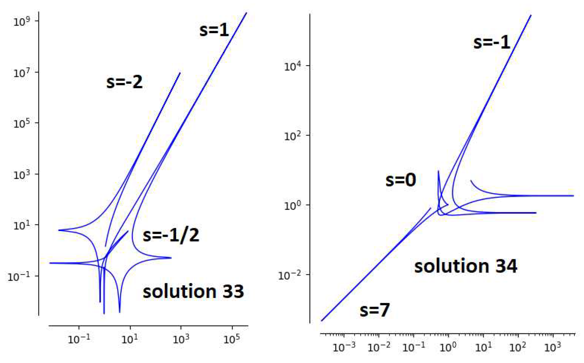
4.4. Two extra icosahedral solutions
5. Discussion
5.1. Application to character varieties of finitely generated groups
Our interest in Painlevé VI arises from our exploration of representations of finitely generated groups encountered in models of topological quantum computing (TQC) [1,17] and the investigation of DNA/RNA short sequences crucial in transcriptomics [2,18]. A model of TQC can commence with a link such as the Hopf link , whose character variety is the Cayley cubic surface [4]. This surface is associated with the Picard solution of , as mentioned at the end of the introduction. Other links, such as or [1], Figure 2, whose character varieties contain the Fricke-Painlevé surfaces for and 3 can be utilized. To these surfaces one can attach solution 30 of Painlevé VI (see subsection 3.5 for the former case), and solutions 20 or 45 (see subsection 3.3 for the latter case).
It has been observed that the Groebner basis of four-letter groups encountered in the context of DNA/RNA sequences contains algebraic surfaces for and 4 as mentioned above, as well as the surface [2]. This surface corresponds to Fricke-Painlevé solution 31, with parameters , associated with the symmetry of the great dodecahedron (see subsection 3.4). The surface with parameters is also part of the Groebner basis for four-letter groups. This reveals that many algebraic solutions of , the Picard solution for the Cayley cubic , solutions 20 and 45 associated to , solutions 3, 21 and 42 for parameters and the great dodecahedron solution 31 should play a role in genetics at the genome scale.
5.2. Perspectives
Isomonodromic deformation is a concept dating back to the nineteenth century, pioneered by P. Painlev’ and subsequently studied by Fuchs, Schlesinger, Jimbo, and numerous other scholars [19]. This concept is underpinned by crucial mathematical properties of isomonodromy equations, including the Painlev’ property, indicating that essential singularities remain fixed while poles may shift; transcendence, implying that solutions are non-classical; the existence of a symplectic structure, a twistor structure, and a Gauss-Manin connection. Isomonodromic deformation finds applications across various fields, such as random matrix theory, statistical physics, topological quantum field theory, nonlinear partial differential equations, Einstein field equations, and mirror symmetry.
While this paper primarily delves into the exploration of algebraic solutions of the Painlev’ VI equation, it is noteworthy that the chaotic dynamics of has also received attention [20]. Further generalizations can be explored, as presented in [21]. In this latter paper, the role of is assumed by a differential equation governing the divergences in a formulation of renormalization in quantum field theory. The concept of a flat connection on a fiber bundle over the three-punctured sphere is significantly extended to a `flat equisingular bundle’ within a tensor category. The underlying symmetries are no longer discrete but are described by a motivic Galois group, also referred to as the `cosmic Galois group’, in line with ’Cartier’s dream’ [22].
Author Contributions
Conceptualization, M.P. and K.I.; methodology, M.P. and D.C.; software, M.P.; validation, D.C.; formal analysis, M.P.; investigation, M.P. and D.C.; writing—original draft preparation, M.P.; writing—review and editing, M.P.; visualization, D.C.; supervision, M.P. and K.I.; project administration, M.P.; funding acquisition, K.I. All authors have read and agreed to the published version of the manuscript.
Funding
Funding was obtained from Quantum Gravity Research in Los Angeles, CA.
Institutional Review Board Statement
Not applicable.
Informed Consent Statement
Not Applicable.
Data Availability Statement
Computational data are available from the authors.
Acknowledgments
The first author would like to acknowledge the contribution of the COST Action CA21169, supported by COST (European Cooperation in Science and Technology).
Conflicts of Interest
The authors declare no conflict of interest.
References
- Planat, M.; Chester, D.; Amaral, M.; Irwin, K. Fricke topological qubits. Quant. Rep. 2022, 4, 523–532. [Google Scholar] [CrossRef]
- Planat, M.; Amaral, M.; Irwin, K. Algebraic morphology of DNA-RNA transcription and regulation. Symmetry 2023, 15, 770. [Google Scholar] [CrossRef]
- Asselmeyer-Maluga, T. Topological quantum computing and 3-manifolds. Quant. Rep. 2021, 3, 153. [Google Scholar] [CrossRef]
- Boalch, P. From Klein to Painlevé via Fourier, Laplace and Jimbo. Proc. Lond. Math. Soc. 2005, 90, 167–208. [Google Scholar] [CrossRef]
- Goldman, W.M. Trace coordinates on Fricke spaces of some simple hyperbolic surfaces. In Handbook of Teichmüller theory, Eur. Math. Soc. 2009, 13, 611–684. [Google Scholar]
- Cantat, S. Bers and Hénon, Painlevé and Schrödinger. Duke Math. J. 2009, 149, 411–460. [Google Scholar] [CrossRef]
- Benedetto, R.L.; Goldman, W.M. The topology of the relative character varieties of a quadruply-punctured sphere. Experiment. Math. 1999, 8, 85–103. [Google Scholar] [CrossRef]
- Iwasaki, K. An area-preserving action of the modular group on cubic surfaces and the Painlevé VI. Comm. Math. Phys. 2003, 242, 185–219. [Google Scholar] [CrossRef]
- Inaba, M.; Iwasaki, K.; Saito, M.H. Dynamics of the sixth Painlevé equation. arXiv 2005, arXiv:math.AG/0501007. [Google Scholar]
- Lisovyy, O.; Tykhyy, Y. Algebraic solutions of the sixth Painlevé equation. J. Geom. Phys. 2014, 124–163. [Google Scholar] [CrossRef]
- Mazzocco, M. Picard and Chazy solutions to the Painlev’ VI equation. Math. Annal. 2001, 321, 157–195. [Google Scholar] [CrossRef]
- Boalch, P. Towards a nonlinear Schwarz’s list. arXiv 2007, arXiv:0707.3375. [Google Scholar]
- Boalch, P. The fifty-two icosahedral solutions of Painlevé VI. J. reine angew. Math. 2006, 596, 183–214. [Google Scholar] [CrossRef]
- Dubrovin, B.; Mazzocco. Monodromy of certain Painlevé-VI transcendents and reflection groups. Invent. Math. 2000, 141, 55–147. [Google Scholar] [CrossRef]
- Hitchin, N. A lecture on the octahedron. Bull. London Math. Soc. 2003, 35, 577–600. [Google Scholar] [CrossRef]
- Kitaev, A.V. Remarks towards the classification of RS42(3)-transformations and algebraic solutions of the sixth Painlevé equation. Semin. Congr. Soc. Math. France 2006, 14, 199–227. [Google Scholar]
- Planat, M.; Amaral, M.M.; Fang, F.; Chester, D.; Aschheim, R.; Irwin, K. Character varieties and algebraic surfaces for the topology of quantum computing. Symmetry 2022, 14, 915. [Google Scholar] [CrossRef]
- Planat, M.; Amaral, M. M.; Chester, D.; Irwin, K. SL(2,C) scheme processsing of singularities in quantum computing and genetics. Axioms 2023, 12, 233. [Google Scholar] [CrossRef]
- Isomonodromic deformation. Available online: https://en.wikipedia.org/wiki/Isomonodromic_deformation (accessed on 1 August 2023).
- Cantat, S.; Loray, F. Holomorphic dynamics, Painlevé VI equation and character varieties. arXiv 2007, arXiv:1207.0154. [Google Scholar]
- Connes, A.; Marcolli, M. Quantum fieds and motives. J. Geom. Phys. 2006, 56, 55–85. [Google Scholar] [CrossRef]
- Cartier, P. A mad day’s work: from Grothendieck to Connes and Kontsevich. The evolution of concepts of space and symmetry. Bull. Amer. Math. Soc. 2001, 38, 389–408. [Google Scholar] [CrossRef]
Figure 1.
Left: Parametric plot for the modulus of Klein solution of (solution 8 of [10], p 157), the discontinuities of the plot correspond to the four poles. Right: the corresponding cubic surface .
Figure 1.
Left: Parametric plot for the modulus of Klein solution of (solution 8 of [10], p 157), the discontinuities of the plot correspond to the four poles. Right: the corresponding cubic surface .
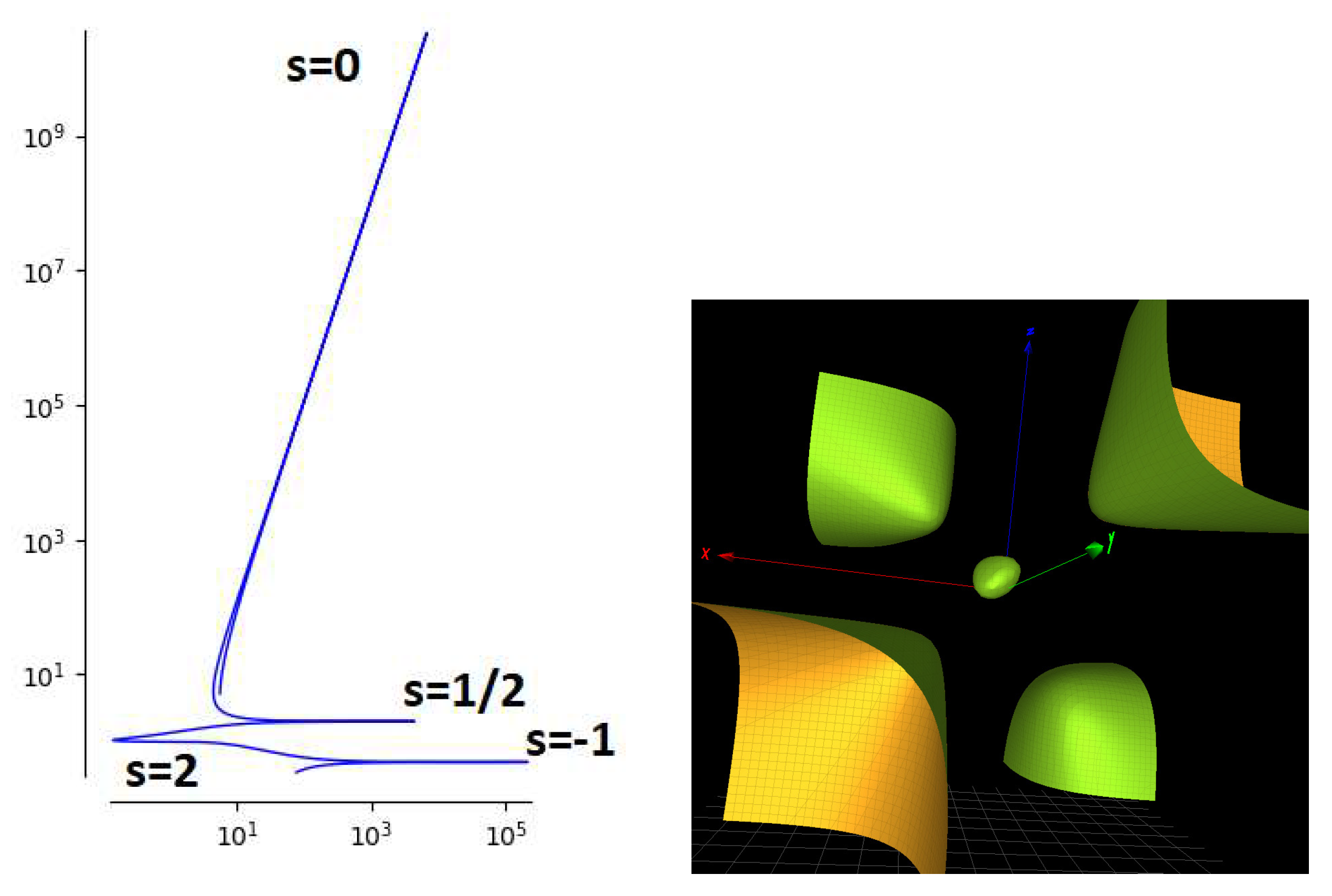
Figure 2.
Solutions related to the algebraic surface are indexed in [10]. Up left: the tetrahedral solution 3, up right: solution 21, middle: modulus of solution 42, down: the corresponding algebraic surface. It is a degree 3 del Pezzo surface of the type.
Figure 2.
Solutions related to the algebraic surface are indexed in [10]. Up left: the tetrahedral solution 3, up right: solution 21, middle: modulus of solution 42, down: the corresponding algebraic surface. It is a degree 3 del Pezzo surface of the type.
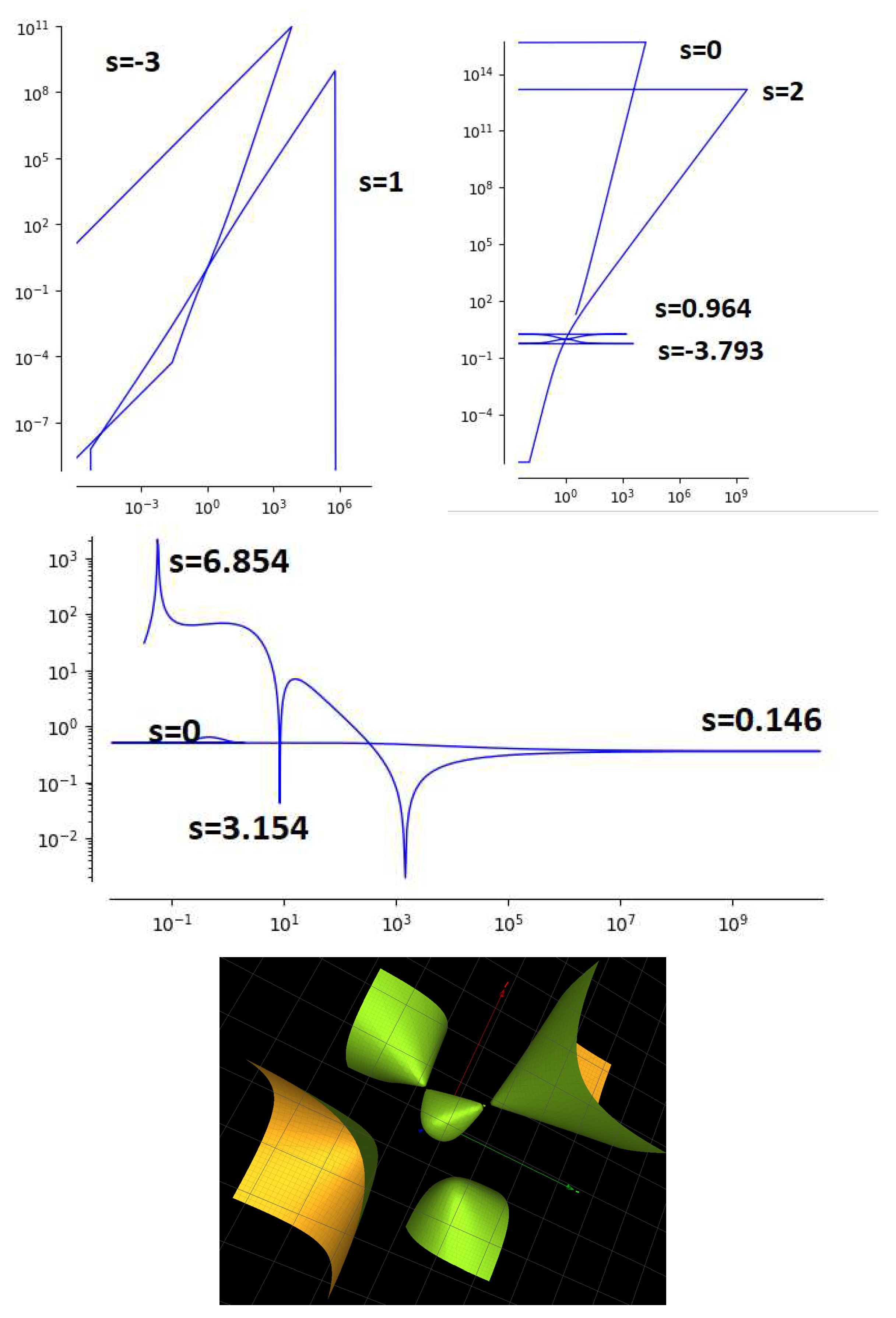
Figure 3.
Solutions related to the algebraic surface are indexed in [10]. Up left: the modulus of the octahedral solution 20, up right: the modulus of solution 45, down: the corresponding algebraic surface.
Figure 3.
Solutions related to the algebraic surface are indexed in [10]. Up left: the modulus of the octahedral solution 20, up right: the modulus of solution 45, down: the corresponding algebraic surface.
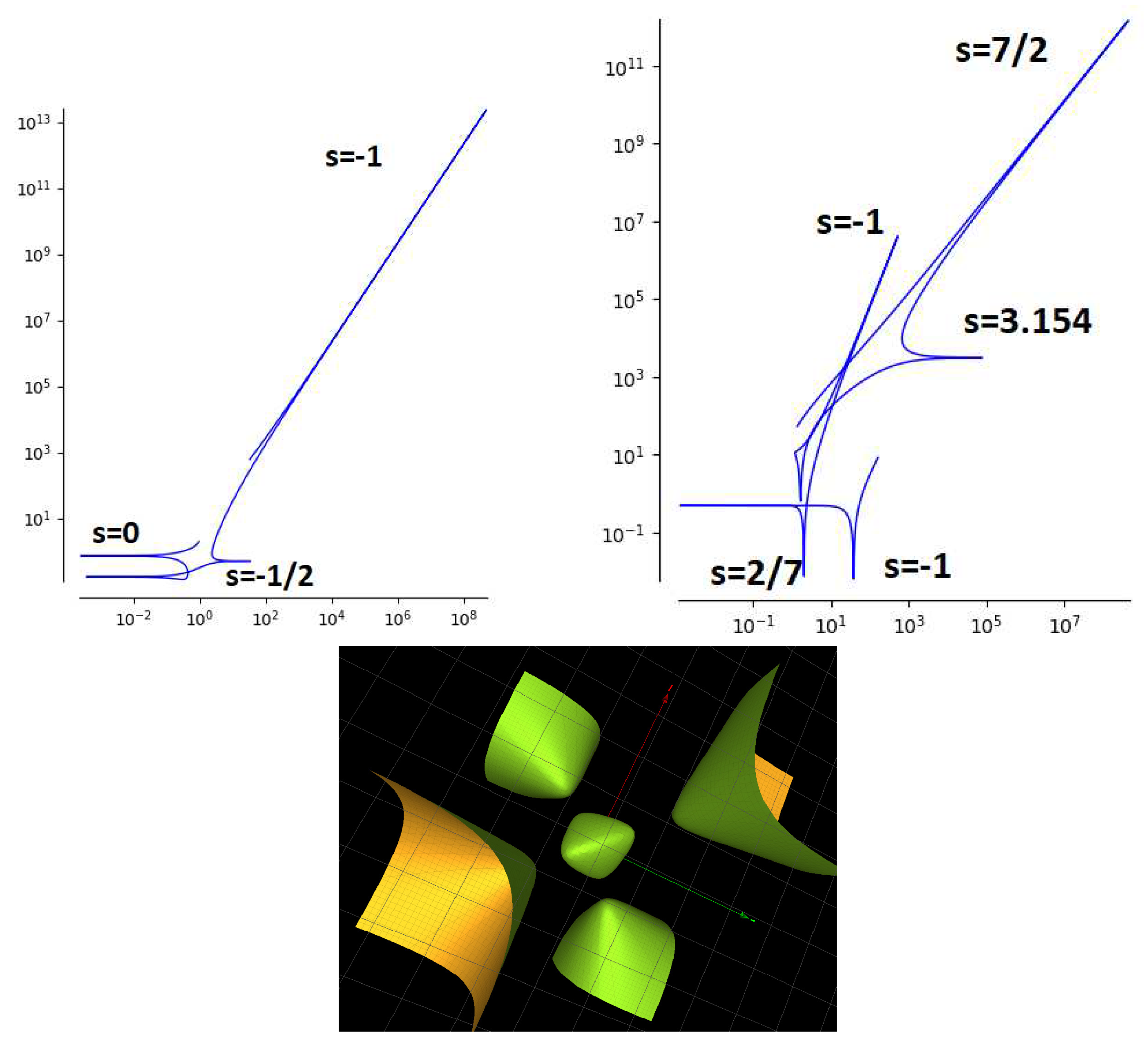
Figure 4.
Left: Parametric plot for the modulus of the great dodecahedron solution of (solution 31 of [10], p 157), the three poles are identified. Right: the corresponding cubic surface is a degree 3 del Pezzo surface of type that is with three isolated singularities).
Figure 4.
Left: Parametric plot for the modulus of the great dodecahedron solution of (solution 31 of [10], p 157), the three poles are identified. Right: the corresponding cubic surface is a degree 3 del Pezzo surface of type that is with three isolated singularities).
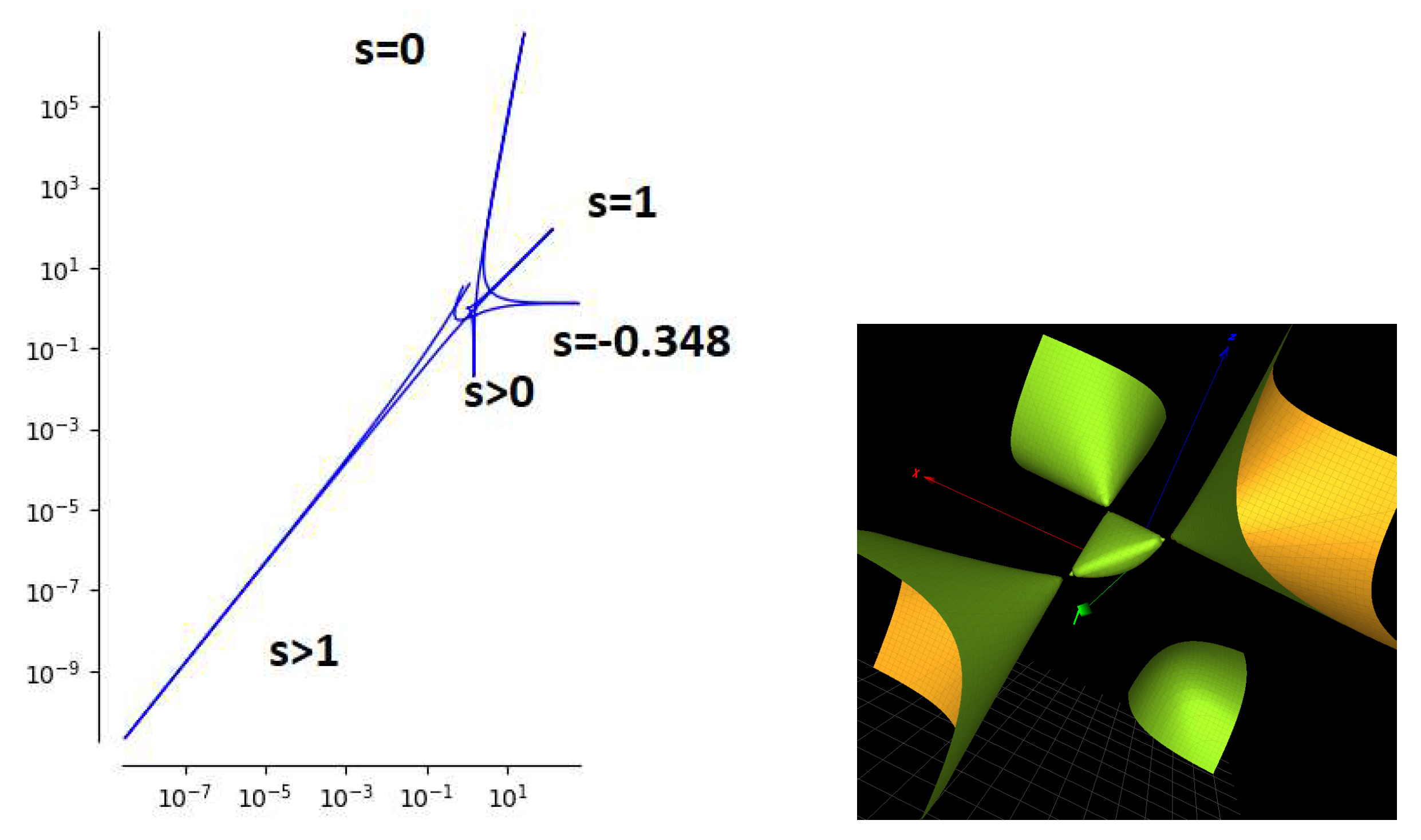
Figure 5.
Parametric plots for the modulus of solutions 1 (with 5 branches: Fricke-Painlevé form ), 30 (an octahedral solution with 16 branches: Fricke-Painlevé form ) and 39 (a Valentiner solution with 24 branches: Fricke-Painlevé form .
Figure 5.
Parametric plots for the modulus of solutions 1 (with 5 branches: Fricke-Painlevé form ), 30 (an octahedral solution with 16 branches: Fricke-Painlevé form ) and 39 (a Valentiner solution with 24 branches: Fricke-Painlevé form .
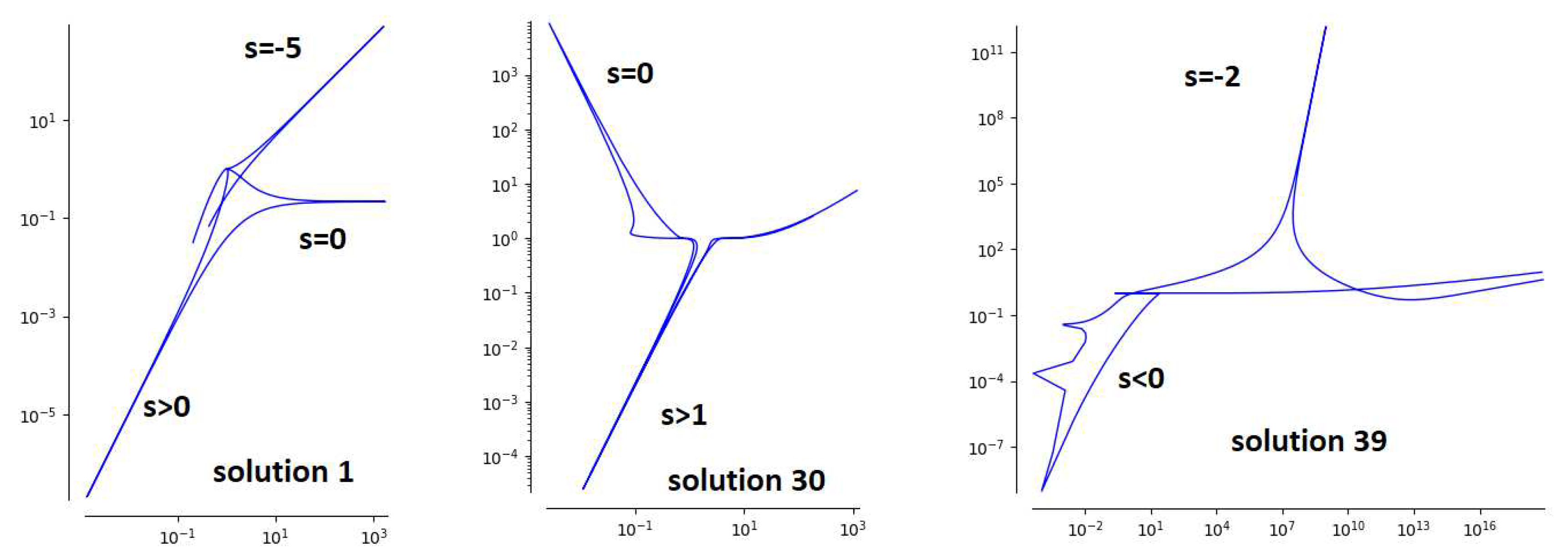
Figure 6.
Left: Parametric plot of an icosahedral solution of (solution 7 of [10], p 157), the discontinuities of the plot correspond to the poles. Right: the corresponding cubic surface.
Figure 6.
Left: Parametric plot of an icosahedral solution of (solution 7 of [10], p 157), the discontinuities of the plot correspond to the poles. Right: the corresponding cubic surface.
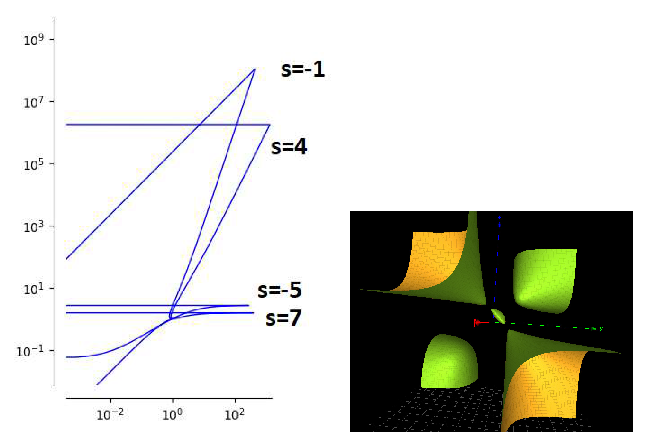
Figure 7.
Parametric plots for the modulus of solutions III (the tetrahedral solution), IV (the dihedral solution), solutions 16 and 17 (icosahedral solutions) as first described in [14]. For the later two solutions, we find poles located at irrational values , , and .
Figure 7.
Parametric plots for the modulus of solutions III (the tetrahedral solution), IV (the dihedral solution), solutions 16 and 17 (icosahedral solutions) as first described in [14]. For the later two solutions, we find poles located at irrational values , , and .
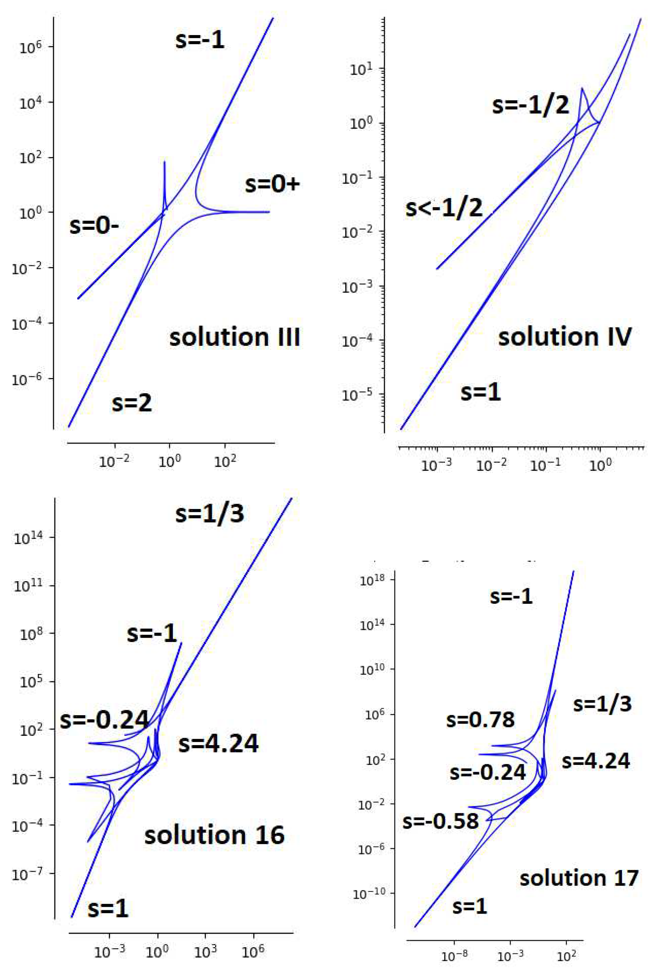
Figure 8.
Parametric plots for the modulus of solutions 26 and 27 that are related to the Valentiner group.
Figure 8.
Parametric plots for the modulus of solutions 26 and 27 that are related to the Valentiner group.
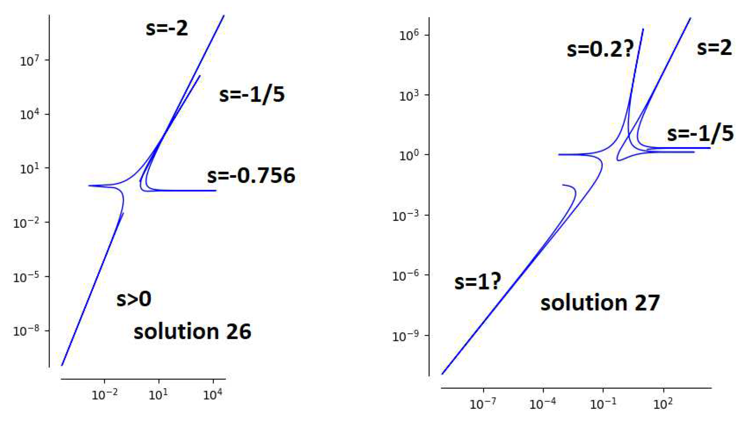
Figure 9.
Parametric plots for the modulus of solutions 33 and 34.
Disclaimer/Publisher’s Note: The statements, opinions and data contained in all publications are solely those of the individual author(s) and contributor(s) and not of MDPI and/or the editor(s). MDPI and/or the editor(s) disclaim responsibility for any injury to people or property resulting from any ideas, methods, instructions or products referred to in the content. |
© 2023 by the authors. Licensee MDPI, Basel, Switzerland. This article is an open access article distributed under the terms and conditions of the Creative Commons Attribution (CC BY) license (http://creativecommons.org/licenses/by/4.0/).
Copyright: This open access article is published under a Creative Commons CC BY 4.0 license, which permit the free download, distribution, and reuse, provided that the author and preprint are cited in any reuse.


