Submitted:
27 November 2023
Posted:
30 November 2023
You are already at the latest version
Abstract
Labyrinth seals are commonly used in turbomachinery in order to control leakage flows. Flutter is one of the most dangerous potential issues for them, leading to High Cycle Fatigue (HCF) life considerations or even mechanical failure. This phenomenon depends on the interaction between aerodynamics and structural dynamics; mainly due to the very high uncertainties regarding the details of the fluid flow through the component, it is very hard to predict accurately. In 2014, as part of the E-Break research project funded by the European Union (EU), an experimental campaign regarding the flutter behaviour of labyrinth seals was conducted at Centro de Tecnologias Aeronauticas (CTA). During this campaign, three realistic seals were tested at different rotational speeds, and the pressure ratio where the flutter onset appeared was determined. The test was reproduced using a linearized uncoupled structural-fluid methodology of analysis based on Computational Fluid Dynamics (CFD) simulations, with results only in moderate agreement with experimental data. A procedure to adjust the CFD simulations to the steady flow measurements was developed. Once this method was applied, the matching between flutter predictions and the measured data improved, but still some discrepancies could be found. Finally, a set of simulations to retain the influence of the external cavities was run, what further improved the agreement with testing data.
Keywords:
aeroelasticity
; flutter
; labyrinth seal
; CFD
; testing
1. Introduction
Leakage flows in the radial gaps between static and rotating parts affect very significantly the performance of turbomachinery. Labyrinth seals are commonly used in order to reduce these flows. These seals are composed of a number of radial fins, which delimit small cavities between them. As a result, leakage flows undergo successive contractions and expansions as they pass through the fin tip or cavity region, leading to substantial losses of stagnation pressure and ultimately to smaller mass flow than a simple slot. The performance of the component is noticeably difficult to predict accurately, in part due to the complexity of the flow (regions with very different Mach numbers, complex vortex structures and separated flow), and in part due to the very high sensitivity to manufacturing tolerances (typical gap values are in the 0.1-0.4 mm range).
One potentially severe issue that labyrinth seals may find is flutter, as documented decades ago by Lewis et al. [1]. Their research illustrates how vibration induced by aeroelastic instabilities may lead to the mechanical failure of the seal. The phenomenon has been studied by a number of authors, beginning with the works of Ehrich [2] and Alford [3], which provide a conceptual description of the problem and formulate simplified analytical models. Some years later, Abbot confirmed some of their main conclusions with experimental and numerical studies [4]. Thanks to the increase in computational power, the past decade saw the appearance of some analysis based on CFD simulations, often supported with additional experimental studies, such as those from di Mare et al. [5] and Miura et al. [6]. However, some authors such as Corral, Vega and Greco [7,8,9] continued with the analytical research of the phenomenon developing a new simplified model that describe the physics of the problem more accurately than its predecessors.
Additionally, in the past years there has been a growing interest in the industry about the topic, with different EU research projects focused on experimental campaigns in order to provide more insight into the phenomenon and produce a good quality data for numerical methods validation. The work presented here takes the testing campaign performed by one of those projects (E-Break) as a reference for a set of CFD based simulations, which successfully reproduce the measurements. One of the main achievements of the simulations is to account for the individual effect of external cavities over the seal structure, an effect that current simplified models ignore.
2. Experimental Set-Up and Procedure
The E-Break (2010-2014) was a collaborative project co-funded by the EU with a work package focused on the study of flutter in labyrinth seals, relying on a comprehensive testing campaign. The main targets of the project were to gain physical understanding of the phenomenon and to provide a good quality set of experimental data, both of stable and unstable cases, to allow the validation of the tools and methodologies of analysis employed by the different partners. For that purpose, an unstable three-fins labyrinth seal was designed to act as reference, and different techniques were employed to stabilize it, including changes in operating point, geometry modifications and the addition of mechanical friction through dampers.
The aforementioned experimental campaign was conducted at Centro de Tecnologías Aeronáuticas (CTA) in Zamudio (Spain), a research institute with more than 20 years of experience in aerodynamic rigs for Low Pressure Turbines. They have also collaborated in other aeroelasticity projects such as FUTURE [10]. These cold flow facilities are designed for turbine rigs testing, usually powered by the air flux provided by the compression system, making it difficult to adapt the facility interface to labyrinth seals testing. This restriction imposed the necessity to install a complete turbine rig to extract energy from the air flux and power the seal, eventually attached to the turbine disk.
The instrumentation of the rig allowed determining both the steady state and the flutter appearance. Regarding the steady field magnitudes, the seal mass flow, static pressure at both inter-fin and external (inlet/outlet) cavities, static temperatures and the shaft speed were recorded to describe the seal operating point. In regards to the unsteady magnitudes, dynamic pressure sensors were located in the inter-fin cavities and a number of dynamic strain gauges were installed in the seal specimen in order to monitor the vibration amplitudes and detect the flutter onset. A sketch of the rig and instrumentation positioning is shown in Figure 1.
Two main parameters were controlled while testing, namely, the rotation speed of the disk and the feed pressure to the high-pressure chamber. The testing procedure, described in Figure 2, consisted in setting the rotation speed of the disk to a chosen value, which will be kept constant thereafter, imposing a zero mass flow state (i.e. set the feeding pressure to ambient value), and then increasing the feeding pressure giving small steps. After each of these steps, a time to reach a stable regime was waited and then the different sensor’s measurements recorded. The process was repeated until the strain gauges were able to detect vibration amplitudes above the established safety limits, moment at which the test was concluded. For each of the instabilities observed, the operating conditions, vibration frequency, nodal diameter (ND) and traveling wave sense were determined, allowing an easy comparison with the numerical results.
Three different seal geometries were tested, depicted in Figure 3. The first specimen, which will be referred as baseline, is a three-fin geometry that corresponds to the aforementioned unstable seal selected for this project. The two additional seals were the result of different modifications applied to the baseline geometry. The first modification consisted on a widening of the seal arm, increasing its minimum width from 3 mm to 5 mm. The second modification consisted on removing the last fin of the baseline seal, essentially a cut to the fin head, yielding a two fins and single cavity seal. The former modification will be referred as robust seal; while the latter will be called two-fin geometry. It has to be mentioned that we will only present simulation results for the baseline and two-fin geometries in this paper.
3. Methodology
The methodology employed in the flutter calculations presented here rely on a linearized uncoupled formulation of the unsteady vibration problem [11] (See Figure 4). This approach, widespread in the industry, simplifies the problem and significantly reduces the computational cost. Two main assumptions are behind this methodology. First, we consider that aeroelastic modes are essentially the same as the purely structural modes. Second, to linearize the unsteady problem equations, we assume that vibration amplitudes are small enough so that the fluid field can be decomposed in a base field plus a series of small perturbations. From the operational point of view, it involves performing a modal analysis of the structure to obtain the modal displacements and frequencies, a non-linear steady CFD simulation that will act as the base solution for the linearized problem, and finally an unsteady linearized CFD simulation where the previously calculated modal shapes and frequencies are imposed. As a result an unsteady pressure field is obtained that, together with the modal displacements, eventually allows computing the work per cycle over the structural displacements imposed. The sign of that work per cycle will determine the stability of the mode.
The structural modes are obtained with a 3-dimensional pre-stressed modal analysis performed with our in-house solver Xipetotec [12]. To reduce the computational cost, the solid domain analysed consists in a sector of 18 degrees, small enough to study the nodal diameters of interest. The mesh has been generated as a 30 planes circumferential extrusion of a 2-dimensional grid, to yield a mesh made of tetrahedrons with about 130,000 nodes (see Figure 5a). Regarding boundary conditions, depicted in Figure 5b, it should be mentioned that cyclic symmetry is employed (orange and fuchsia faces), shaft rotation imposed, aerodynamic loads considered over every wetted surface (transparent faces) and a series of displacement constraints imposed to model the seal attachment to the disk. Specifically, axial displacements have been restricted in all the face of contact between seal and disk (blue face) and a 3-degrees of freedom punctual constraint has been added to simulate the bolt.
The steady fluid problem is solved with ITP’s CFD code Mu²s²t [13], a solver for the fully non-linear RANS equations which counts with a linearized version that allows to solve the unsteady vibration problem with a pseudo time marching scheme. The solver, capable of running in GPUs [14], has been well validated over time and is routinely employed at ITP to support its aerodynamic designs and perform either aeroelastic or aeroacoustics simulations. In the work presented here, a two equations k-w turbulence model has been chosen, with frozen turbulence variables in the unsteady simulation. It is important to highlight that a simulation without turbulence model will not achieve a steady solution in this kind of configuration. Other authors have considered full DNS simulations of the seal flow, with fairly good matching of their experimental data. Nevertheless, this approach is incompatible with obtaining a proper steady solution and studying linear perturbations from that state, which is our current to the flutter study, as mentioned before.
Regarding boundary conditions, walls were modelled as adiabatic with non-slip condition and fluid magnitudes at inlet (total pressure and temperature) and outlet (static pressure) are taken from experimental measurements. Finally, flow direction at inlet was set as normal to boundary.
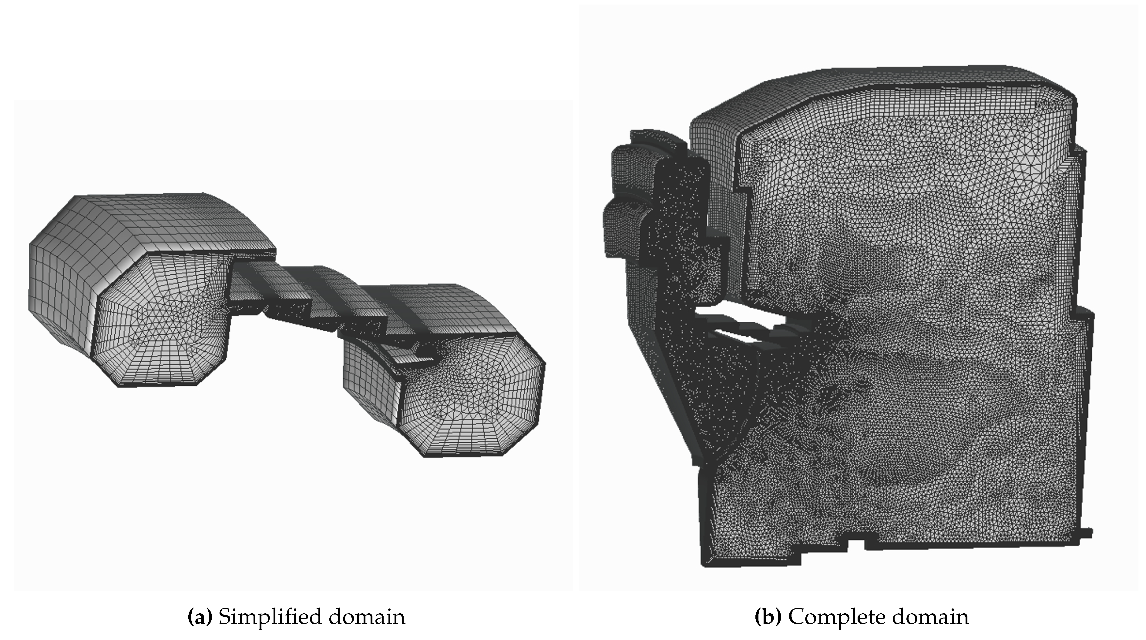
The computational 3D grid has been built from a 2D-hybrid mesh, with layers of quad elements in the viscous region next to the walls and triangle elements in the inviscid region, extruded in the circumferential direction to yield an 18 degrees sector. Phase-shifted boundary conditions are applied in the lateral boundary faces of the fluid domain. Two different domains have been simulated, namely, a simplified version focused on the seal head and neglecting external cavities, and a complete domain considering the full testing geometry. Details about the resulting grids can be seen in Table 1.
Figure 6.
CFD domains simulated and associated grids.
4. Results and Discussion
4.1. Modal analysis
As mentioned in the previous section, the uncoupled methodology requires a modal analysis of the structure to obtain its modal characteristics that will be imposed in the linearized CFD simulation. The structural analysis of the two specimen of study, namely the baseline and two-fin configurations, yields the frequency curves shown in Figure 7. As expected, the two-fin seal exhibits higher frequencies than the baseline configuration, mainly due to its lower mass at the fin head. This result will have important implications regarding the stability, as we will discuss later on. The other key feature that should be pointed out is the trend of the curves. As the reader can observe, the behaviour of the frequency against the nodal diameter is very similar to that found in disk modes, what should not be a surprise given the kind of structure we are analysing. It is well known that increasing the nodal diameter number imposes more restrictions to the disk displacements, which in turn produce a stiffening effect in the structure and an increase in the natural frequencies. It has to be mentioned that measured instabilities show discrepancies of 2-3% in frequency when compared with the predicted values, which is considered acceptable.
Figure 8 and Figure 9 depict the modal shapes for different nodal diameters. We can observe that two main components exist, namely, an edge-wise component that is dominant at low NDs and a torsion component that is dominant at high NDs. It is important to mention that the torsion component can be defined as a rotation of the seal head around a pivot point located close to the junction between the seal arm and head. The position of that pivot point is of vital importance from the stability point of view, as we will discuss in the results section.
4.2. Steady flow
Steady flow in labyrinth seals exhibit a very complex structure with different vortices filling the cavities. Despite this complexity, there are two main regions to consider as depicted in Figure 10:
- The flow inside the cavities (both inner seal cavities and outer cavities) is a low velocity flow. Ignoring the swirl, the meridional Mach number is approximately 0.1 in that region. The static pressure is roughly uniform inside each of the cavities.
- The flow in the tip gaps has much higher Mach number, with the last fin being essentially choked in the vast majority of operation points. This is the region responsible of most of the pressure losses in the seal.
- A remarkable feature of the flow in the tip gaps is the re-circulation bubble that often appears. This bubble varies in size depending on the operation point, but usually affects a significant part (around 25%) of the gap. In practice, this leads to a significant reduction in the effective gap, leading to smaller mass-flow through the seal than could be expected from the nominal gap under ideal conditions.
The aforementioned characteristics make the CFD simulations more challenging than in other turbine elements such as the blades. The extremely different length and time scales associated to the gaps and cavities regions are not the ideal conditions for numerical codes. Moreover, boundary layers in the fin gaps should be well captured due to its relevance in the results (i.e. re-circulation bubble size and mass flow), imposing severe restrictions to the mesh in the region. Finally, convergence in the low speed regions of the external cavities can be slow, especially for the thermal part of the problem, being advisable to use an initial solution with a reasonable temperatures field.
When comparing the measurements obtained in the experimental campaign with the predictions obtained with the aforementioned methodology, non-negligible discrepancies may be found. There are several possible sources for these discrepancies:
- Deformation of the rotating seal due to the steady loading (centrifugal forces and pressure differences). Depending on the operation conditions, this effect may account for gap differences up to 10μm.
- Manufacturing and/or positioning tolerances changing the gap value from the nominal one.
- Mismatch between the CFD predictions and the real flow structure. RANS simulations are inherently limited when dealing with complex flows, and even small errors in the prediction of the size of the re-circulation bubble at the fin tips or the turbulent viscosity in that region can affect significantly the mass flow prediction.
- Rubbing or contact between the rotating seal and the stator, that can cause damage both parts and increase the gaps.
In our particular case, static deformations are small when compared with the nominal gaps of 0.3mm. Therefore, their impact on the steady field should not be high. However, notice that even if that is the case, as static deformations tend to close the gaps, and as our CFD results with nominal gaps are already giving lower mass flow than measured in the experiments, including this small gap corrections (closures) in the simulations will increase the mismatching found. Other remarkable point is that discrepancies found depend on the operating point, what makes us think that the term associated to the CFD (RANS) limitations when calculating the re-circulation bubble has a non-negligible importance, at least as important as manufacturing or assembling tolerances. However, that term alone does not justify differences up to 20% in mass flow, and does not explain why those differences are much smaller for the two-fin seal.
Having said that, the only explanation left is the rubbing. There was evidence of rubbing appearing during the tests leading to a gaps widening, what will perfectly explain why the experimental mass flow was higher than the calculated by the CFD. Other interesting point is that, as both static and dynamic displacements are higher for the baseline geometry than for the two-fin seal, it is fair to think that contacts will be more severe in the former, explaining why we are not finding the same level of discrepancies for both seals. However, although rubbing was detected, it was not quantified how much it affected to the gaps not allowing us to use that information to correctly model the actual geometry in our simulations.

Table 2.
Discrepancies between CFD steady simulations (nominal gaps of 0.3mm) and experimental data.
Table 2.
Discrepancies between CFD steady simulations (nominal gaps of 0.3mm) and experimental data.
| Configuration | Ω (r.p.m.) | ΔP (MPa) | Err. | Err. | Err. |
|---|---|---|---|---|---|
| Baseline | 0 | 0.1674 | -23.18 % | 3.31 % | 9.81 % |
| 1500 | 0.1513 | -22.46 % | 3.56 % | 10.6 % | |
| 2200 | 0.1392 | -20.71 % | 3.44 % | 9.80 % | |
| 2900 | 0.1251 | -18.37 % | 2.68 % | 8.11 % | |
| 2 Fins | 0 | 0.1059 | -2.95 % | -1.14 % | - |
| 1500 | 0.0968 | 19.61 % | -0.89 % | - | |
| 2200 | 0.1037 | -3.21 % | -3.9 % | - | |
| 2900 | 0.1081 | -0.55 % | -2.22 % | - |
At this point, a different approach had to be followed. Instead of imposing the radial gaps, which essentially were unknown due to the contacts between rotor and stator, it makes sense trying to impose the pressure and mass flow as measured and then develop a numerical procedure to adjust the gaps in order to match those steady magnitudes in our CFD. It consisted on a Newton-Raphson iterative method using numerical differentiation to obtain the Jacobian. For a seal with “N” fins, the system of equations to be solved imply “N-1” equations corresponding to the “N-1” cavities pressure, plus an additional equation corresponding to the mass flow, with “N” gap unknowns (see equations 1 and 2):
The different partial derivatives are calculated using numerical differentiation by means of CFD simulations with individually modified gaps (+10% in this particular case). Additionally, a simulation where all the fin gaps are uniformly modified, allows us to calculate the required uniform that would yield the experimental mass flow. Taking these new gaps as reference, the right side part of equation 2 is zero, which simplifies the resolution of the system. The calculated will then be applied to these new reference gaps, not the nominal ones, yielding the final resulting gaps. The process should be repeated until the desired convergence level is reached. It is remarkable how fast the method converged, producing results that were deemed acceptable after a single iteration. The obtained errors both in pressures and mass flow are shown in Table 3.
4.3. Unsteady flow field
In this section, we will focus on the unsteady pressure field obtained from the linearized unsteady problem. Figure 11a and Figure 11b show that most of the activity is located at inter-fin cavities, being the dominant term of the problem. The result is not surprising considering that pressure variations in the cavities occur due to volume and mass flow changes. These two terms should be negligible in outer cavities given its size. However, as we will see later on, outer cavities may exhibit high unsteady pressure levels under certain operating conditions.
Other distinctive feature of the obtained unsteady pressure field is its uniformity inside each of the inter-fin cavities. As expected, the cavity positioned further from the pivot point presents higher pressure levels. However, when we increase the ND number vibration frequencies rise (see Figure 7) and the uniformity of the pressure field breaks. The effect starts to be apparent for ND +5 (see Figure 11b).
4.4. Seal Stability
The most remarkable fact about the experimental campaign is that flutter was found for all the three different seal geometries and every rotational speed tested. Depending on the seal specimen and rotational speed chosen, the pressure drop required to initiate the instability was different. Once flutter appeared, the vibration amplitude could grow really fast as results plotted in Figure 12 show, underlining the importance of a good control system to allow an easy and fast termination of the test.
Comparing results from the baseline and two-fin geometries (Figure 12 and Figure 13), two main differences can be found. First, the two-fin seal becomes unstable at lower pressure ratios than the baseline specimen does, that is, it reaches its unstable region before; second, the vibration amplitudes rise more abruptly in the baseline case, implying a higher absolute aerodynamic damping level (this point is confirmed by CFD simulations, see Figure 14). Summarizing, the two-fin seal reaches its unstable region first, but once we enter that region, the instability itself is less severe than that observed in the baseline configuration.
Both points can be easily related to the modal shapes and frequencies of both seals. Regarding the modal shape, both seals can be considered as high-pressure side supported, that is, the pivot point of the resulting modal displacements lies closer to the high-pressure side of the seal (the right-most side in this case). The careful reader may notice that the two-fin seal is a low-pressure side supported seal actually, but it behaves in the opposite sense as a combination of being inclined and having relatively high axial displacements when compared to the radial ones. The Corral-Vega model for stepped seals ([8]) covers this fact. Thus, as both seals behave as HPS supported seals, the one with higher frequency will be the one closer to the unstable region, according to the Abbot’s criteria. As it was mentioned before, Figure 7 shows that effectively, the two-fin seals is the one with higher modal frequencies.
Finally, regarding the absolute value of the damping itself, it should be taken into account that the baseline configuration has an additional cavity positioned further from the pivot point, thus producing higher unsteady pressure levels and work per cycle. In fact, in the two-fin seal specimen, the pivot point lies somewhere in between the two fins, splitting the inter-fin cavity into two regions that will produce works per cycle with opposite sign, reducing its capability to produce high levels of aerodynamic damping.
Before showing the stability results from the CFD simulations, a couple of clarifications should be made. The first thing to consider is that our simulations do not include any mechanical damping and do not attempt to calculate any vibration amplitude. That kind of study is beyond the scope of this paper. The target of our analysis is to determine whether the seal is aerodynamically unstable when operating at a given condition. This is a necessary but not sufficient condition to have flutter, as mechanical friction could prevent vibration depending on the relative importance of both terms. In addition, when more than a single unstable nodal diameter coexist, the most unstable one (after considering the mechanical damping) tend to prevail. With that in mind, it is not a surprise that simulations predict a wider set of unstable nodal diameters than those detected by the experimental readings. The only thing that can be demanded to simulations of the kind presented here is that the experimentally measured nodal diameters are among the predicted set of unstable ones.
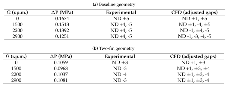
The predicted instabilities by our simplified domain simulations are compared with experimental measurements in Table 4, both for nominal and adjusted gaps. The first point to highlight is that both geometries have been predicted as unstable under all the operating conditions simulated, as it happened in the testing campaign. However, the predicted instabilities are only in moderate agreement with the experiments. Regarding the baseline geometry, even the nominal gaps simulation correctly predicted all the instabilities, although the adjustment procedure modifies the results reducing the list of unstable nodal diameters. In contrast, the two-fin specimen simulations do not match the experimental measurements so well, failing to predict the 0 rpm case and not capturing the traveling wave sign in the 2900 rpm case. It has to be mentioned that the instability at 1500 rpm (ND -3) is well captured only after the gaps adjustment process, even though the gap correction for the two-fin geometry was not too big. This fact emphasizes the necessity to feed the simulations with the right gap values.
All the results shown so far correspond to the simulations performed with the simplified domain (see Figure 6). By simplifying the domain we intend to reduce the computational cost, but at the same time, we are neglecting the effect of outer cavities in the overall stability of the seal. Although this is essentially true in most cases, as unsteady pressure plots in Figure 11 show, external cavities may play a non-negligible role regarding stability under certain circumstances. When vibration frequencies approach the natural frequencies of those cavities, a resonance occurs and noticeably unsteady pressure levels may appear. Moreover, that pressure will act over a wide seal surface, thus having the potential to become the dominant term of the problem. Keeping that in mind, additional simulations using the detailed domain have been run. This domain incorporates the whole seal structure along with the actual external cavities geometry (see Figure 6).
Before going on to comment the stability changes observed in these additional simulations, it is worth to mention that steady state remains almost unaffected and so, previously shown results and discussion regarding steady results still applies. Having said that, the first thing we observe in the unsteady linearized problem solutions is that CFD confirms that the seal vibration is exciting the outer cavities resonances for some nodal diameters, as Figure 15 shows. Moreover, Table 5 indicates that those resonances are able to modify the seal stability, as the list of unstable NDs has changed. The effect is more evident in the two-fin seal, and once again, this fact can be explained by the low damping levels that seal exhibits when compared to the baseline configuration. If the seal head is producing low work per cycle levels, it is easier for external cavities to become the dominant term of the problem.
Regarding the agreement between simulations and experimental stability, we must highlight that the new results obtained for the two-fin geometry (shown in Table 5) perfectly match the experiments in all the operating points analysed. However, for the baseline configuration we obtain mixed results. While we are improving the matching in some aspects, (ND 4 is not predicted as unstable at 0 rpm or ND 5 instability is reduced to the backwards travelling wave, in line with the tests) it seems we are over predicting the effect of external cavities over the ND 4 forward travelling wave, that suffers a complete stabilization at 1500 rpm and 2900 rpm, in contrast with experimental data. A deeper analysis indicates that ND +4 is operating in a region really close to the stability limits. This region is really sensitive to details, with minor changes in the involved parameters producing big changes in damping values, both in sign and magnitude and thus, it is hard to predict by simulations.
Overall, we think the agreement between the detailed simulations (i.e, adjusted gaps and full domain) and experimental data is really good, only failing to predict the aforementioned travelling wave sign of ND 4 instability in baseline configuration.
5. Conclusions
The stability of two realistic labyrinth seal geometries has been analysed with a FEM-CFD uncoupled linear methodology and the results obtained compared with existing experimental data. The nature of typical flow through labyrinth seals represented a challenge for the numerical code, both from the accuracy and convergence points of view. In addition, the uncertainties regarding actual gap values during testing complicated the modelling of the problem even more.
Despite of that, the agreement between simulations and test data is considered reasonably good after applying the gaps adjustment process and including the external cavities, which proved to have a non-negligible impact in the seal stability. Thus, we consider the validity of the proposed methodology is confirmed by the obtained results.
Author Contributions
Conceptualization, J.G.; methodology, J.G. and A.S.; software, A.S.; validation, O.B., A.S. and A.A.; formal analysis, O.B., A.S. and A.A.; investigation, A.P.; resources, J.G. and R.A.; data curation, R.A. and A.P.; writing—original draft preparation, O.B.; writing—review and editing, O.B., J.G., A.S., A.A., R.A. and A.P.; visualization, O.B., R.A. and A.P.; supervision, J.G. and R.A.; project administration, J.G. and R.A.; funding acquisition, J.G. and R.A. All authors have read and agreed to the published version of the manuscript.
Funding
This research was developed inside the collaborative project E-Break co-funded by the European Commission within the 7th Framework Programme (2007-2013), under grant agreement number ACP2-GA-2012-314366-E-BREAK. The APC was funded by Industria de Turbopropulsores SAU (ITP Aero).
Institutional Review Board Statement
Not applicable.
Informed Consent Statement
Not applicable.
Data Availability Statement
The data presented in this study are available on request from the corresponding author.
Acknowledgments
The authors wish to thank ITP Aero for its support and permission to publish this paper, as well as the E-Break project members for enabling this study with its rigorous work and dedication.
Conflicts of Interest
The authors declare no conflict of interest.
Abbreviations & Nomenclature
The following abbreviations are used in this manuscript:
| Latin Symbols | |
| Seal mass flow | |
| g | Fin gap |
| P | Static Pressure |
| Abbreviations | |
| Bw | Backwards travelling wave |
| CFD | Computational Fluid Dynamics |
| DNS | Direct Numerical Simulation |
| Fw | Forwards travelling wave |
| HCF | High-Cycle Fatigue |
| ND | Nodal Diameter |
| RANS | Reynolds Averaged Navier-Stokes equations |
| SG | Strain Gauge |
| Stdn | Standing wave |
| URANS | Unsteady Reynolds Averaged Navier-Stokes equations |
| Greek symbols | |
| Δ | Magnitude variation |
| ξ | Aerodynamic Critical Damping Ratio |
| Ω | Shaft rotational speed |
| Sub-scripts | |
| i | Fin index |
| j | Inter-fin cavity index |
| max | Maximum |
References
- Lewis, D.; Platt, C.; Smith, E. Aeroelastic instability in F100 labyrinth air seals. Journal of Aircraft 1979, 16, 484–490. [Google Scholar] [CrossRef]
- Ehrich, F. Aeroelastic Instability in Labyrinth Seals. Journal of Engineering for Power 1968, 90, 369–374. [Google Scholar] [CrossRef]
- Alford, J.S. Nature, causes, and prevention of labyrinth air seal failures. Journal of Aircraft 1975, 12, 313–318. [Google Scholar] [CrossRef]
- Abbott, D.R. Advances in Labyrinth Seal Aeroelastic Instability Prediction and Prevention. Journal of Engineering for Power 1981, 103, 308–312. [Google Scholar] [CrossRef]
- di Mare, L.; Imregun, M.; Green, J.S.; Sayma, A.I. A Numerical Study of Labyrinth Seal Flutter. Journal of Tribology 2010, 132, 022201. [Google Scholar] [CrossRef]
- Miura, T.; Sakai, N. Numerical and Experimental Studies of Labyrinth Seal Aeroelastic Instability. Journal of Engineering for Gas Turbines and Power 2019, 141, 111005. [Google Scholar] [CrossRef]
- Corral, R.; Vega, A. Conceptual Flutter Analysis of Labyrinth Seals Using Analytical Models. Part I: Theoretical Support. Journal of Turbomachinery 2018, 140, 121006. [Google Scholar] [CrossRef]
- Corral, R.; Vega, A.; Greco, M. Conceptual Flutter Analysis of Stepped Labyrinth Seals. Journal of Engineering for Gas Turbines and Power 2020, 142, 071001. [Google Scholar] [CrossRef]
- Corral, R.; Greco, M.; Vega, A. Higher Order Conceptual Model for Labyrinth Seal Flutter. Journal of Turbomachinery 2021, 143, 071006. [Google Scholar] [CrossRef]
- Corral, R.; Beloki, J.; Calza, P.; Elliott, R. Flutter Generation and Control Using Mistuning in a Turbine Rotating Rig. AIAA Journal 2019, 57, 782–795. [Google Scholar] [CrossRef]
- Corral, R.; Gallardo, J.M.; Vasco, C. Aeroelastic Stability of Welded-in-Pair Low Pressure Turbine Rotor Blades: A Comparative Study Using Linear Methods. Journal of Turbomachinery 2004, 129, 72–83. [Google Scholar] [CrossRef]
- Cordoba, O. FEM Considerations to Simulate Interlocked Bladed Disks With Lagrange Multipliers. Turbo Expo: Power for Land, Sea, and Air; Paper GT2020-15140, ASME: Virtual, Online, 2020; Vol. 10B: Structures and Dynamics, p. V10BT26A009. [CrossRef]
- Corral, R.; Crespo, J.; Gisbert, F. Parallel Multigrid Unstructured Method for the Solution of the Navier-Stokes Equations. 42nd AIAA Aerospace Sciences Meeting and Exhibit; AIAA Paper 2004-0761, AIAA: Reno, NV, 2004. [CrossRef]
- Gisbert, F.; Corral, R.; Pueblas, J. Computation of Turbomachinery Flows with a Parallel Unstructured Mesh Navier-Stokes equations Solver on GPUs. 21st AIAA Computational Fluid Dynamics Conference; AIAA: San Diego, California, 2013. [CrossRef]
Figure 1.
Test rig assembly (Baseline geometry).

Figure 2.
Schematics of testing procedure.
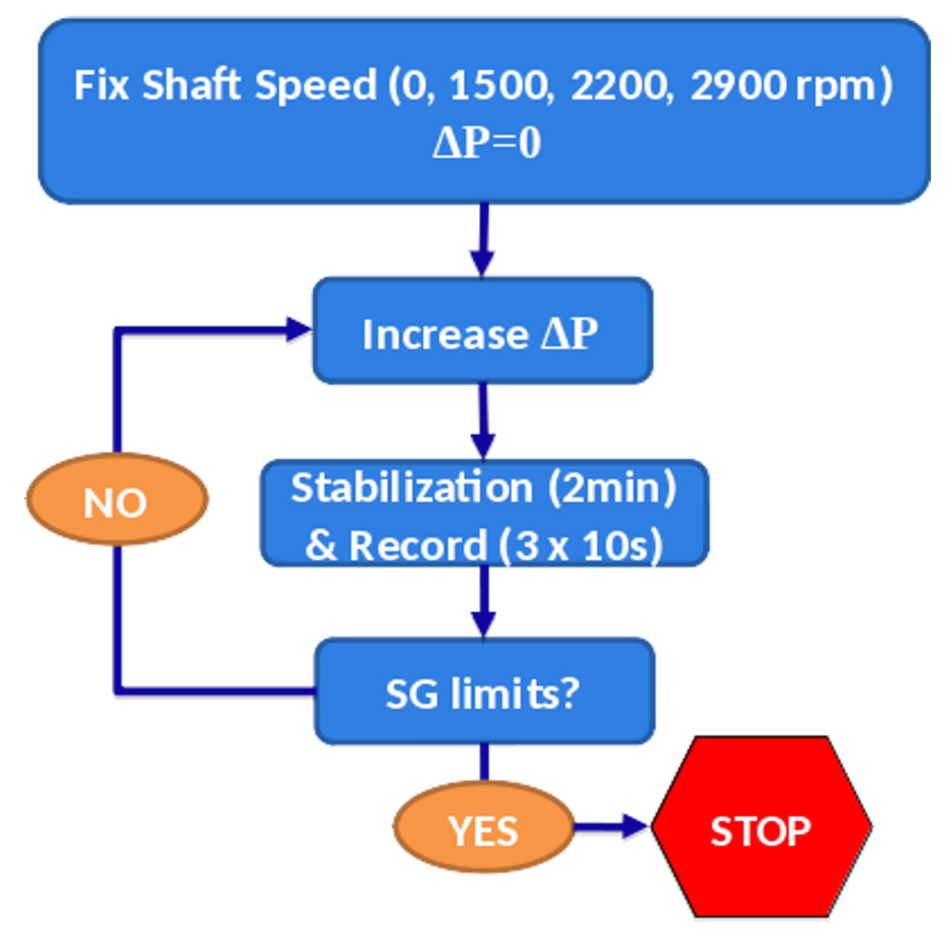
Figure 3.
Geometries tested in the E-Break project.
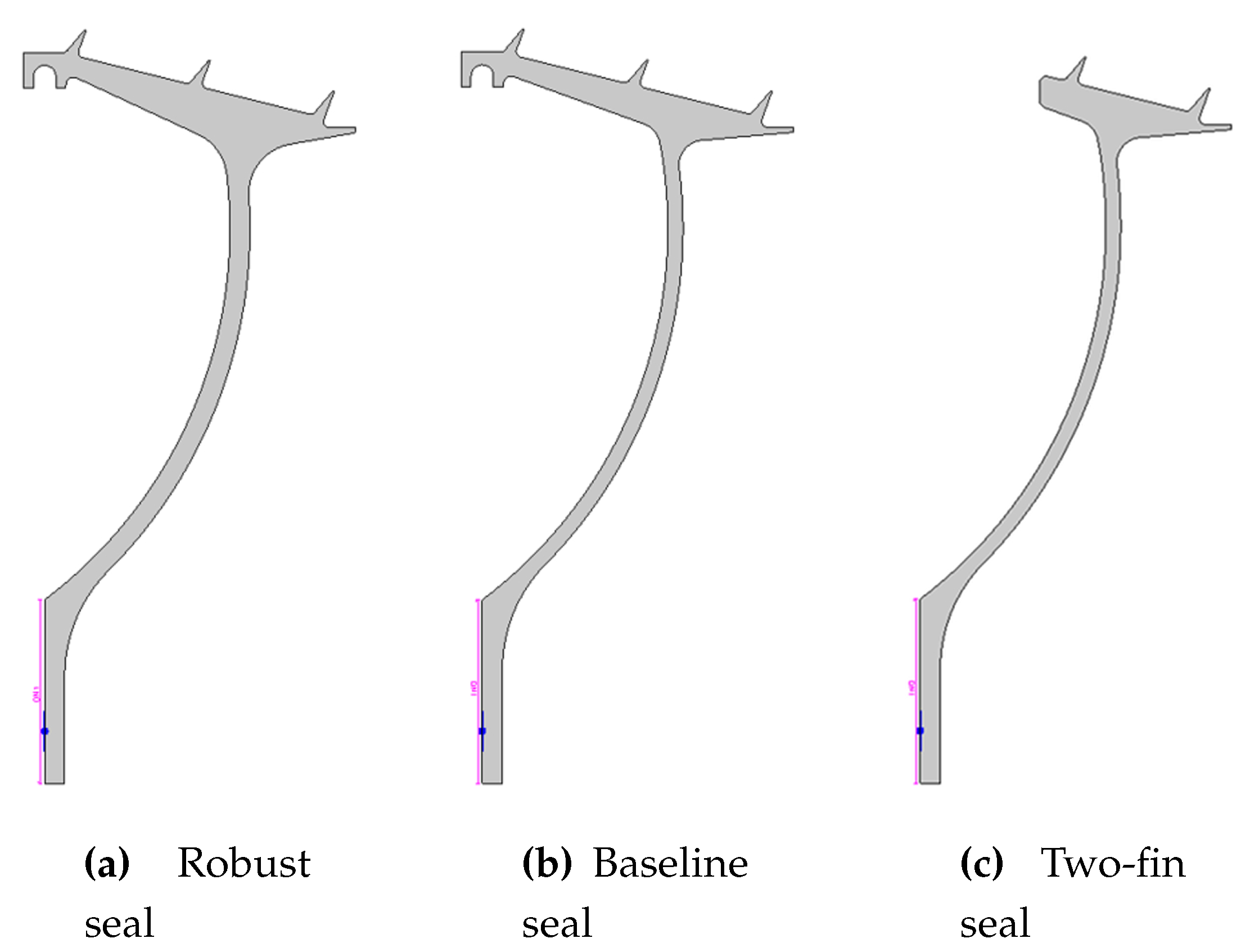
Figure 4.
Uncoupled structural-fluid linearized methodology.
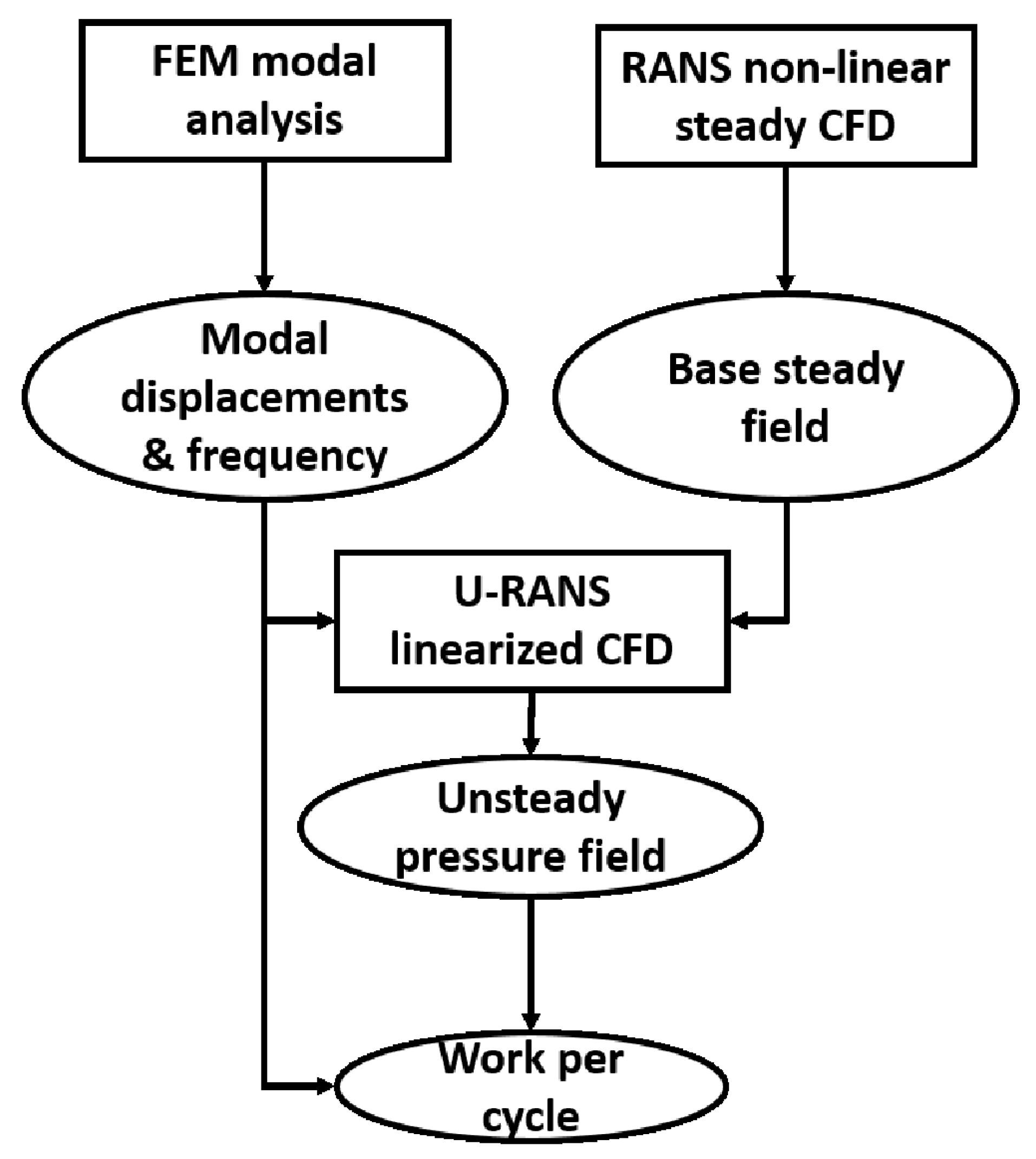
Figure 5.
FEM model mesh and boundary conditions.
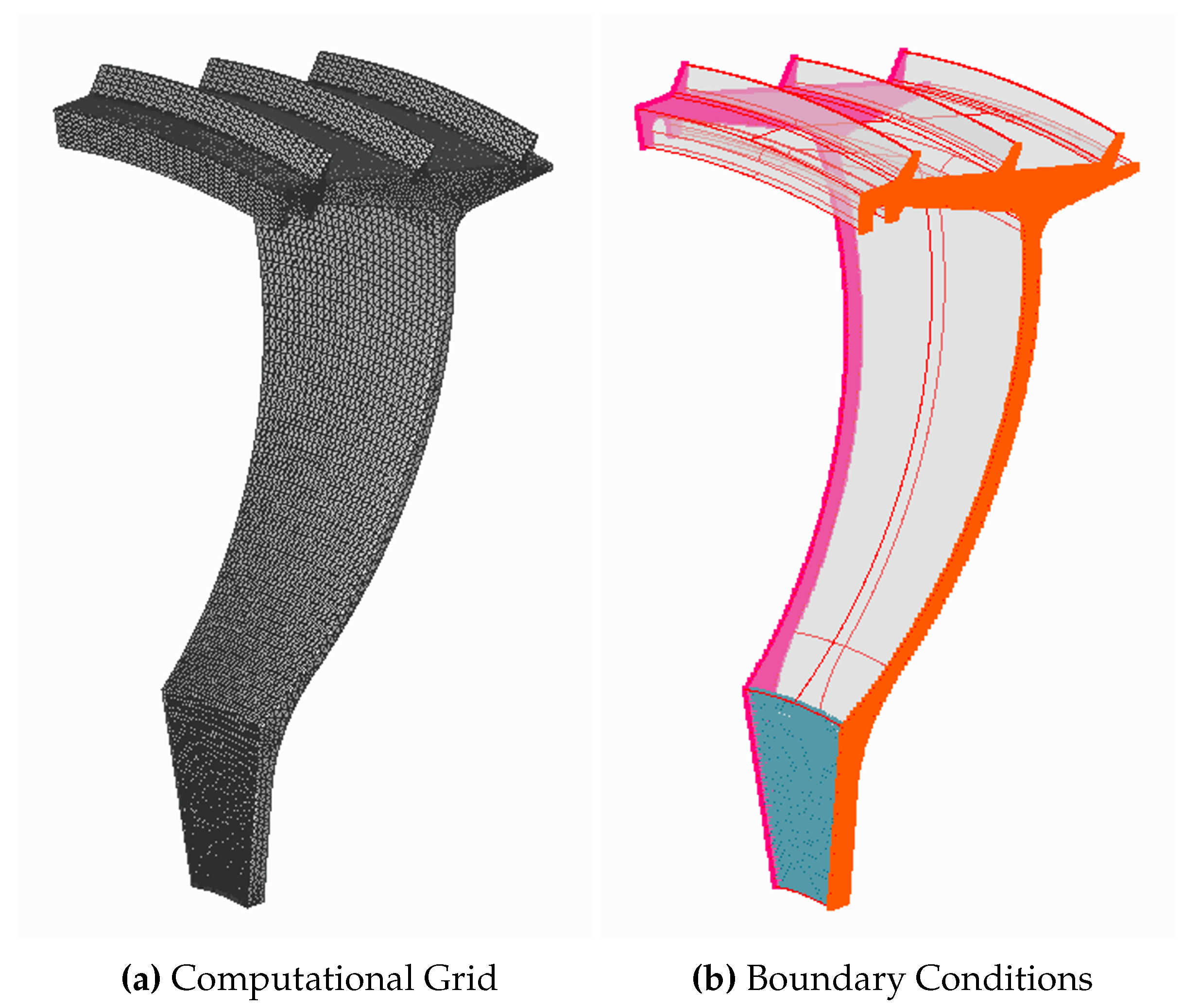
Figure 7.
Modal frequencies at 1500 rpm.
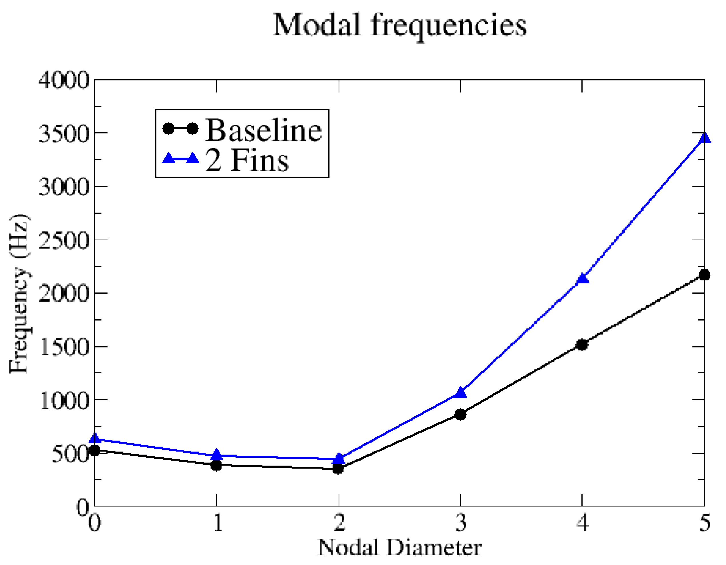
Figure 8.
Modal shapes of the baseline geometry for different Nodal Diameters.
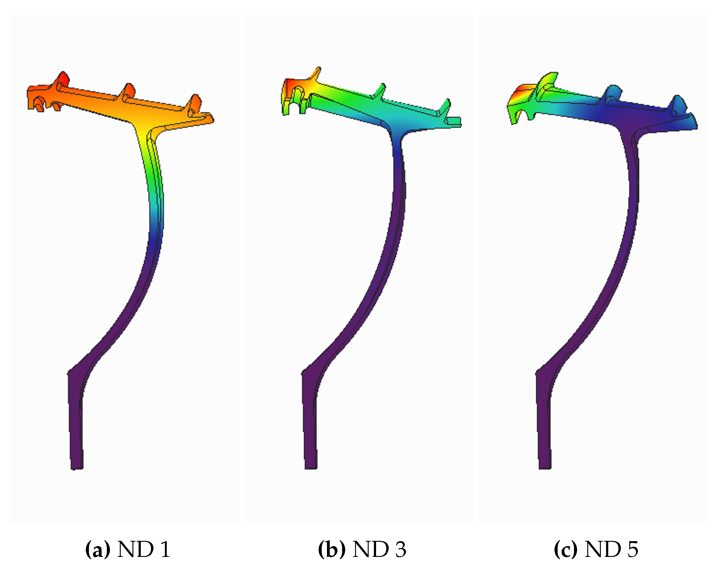
Figure 9.
Modal shapes of the two-fin geometry for different Nodal Diameters.
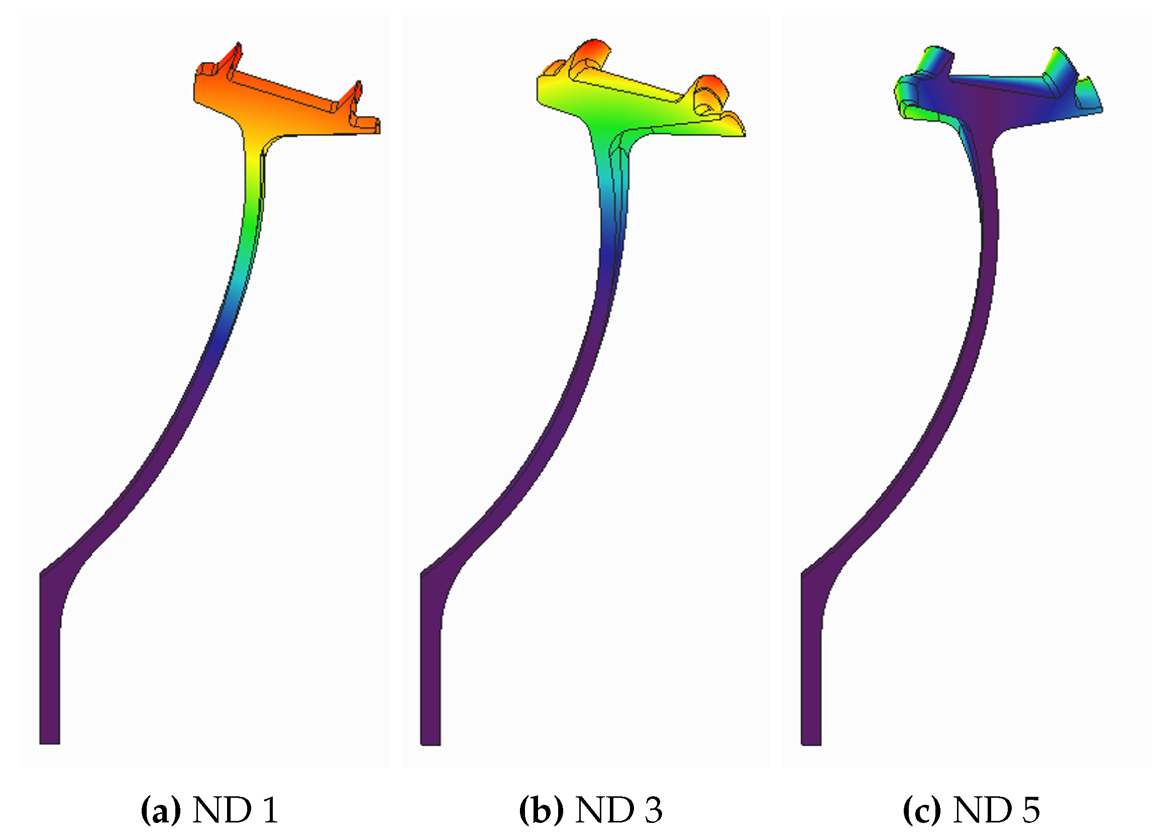
Figure 10.
Steady solution from CFD. Baseline geometry operating at 2900 rpm, ΔP = 0.1251 (MPa).
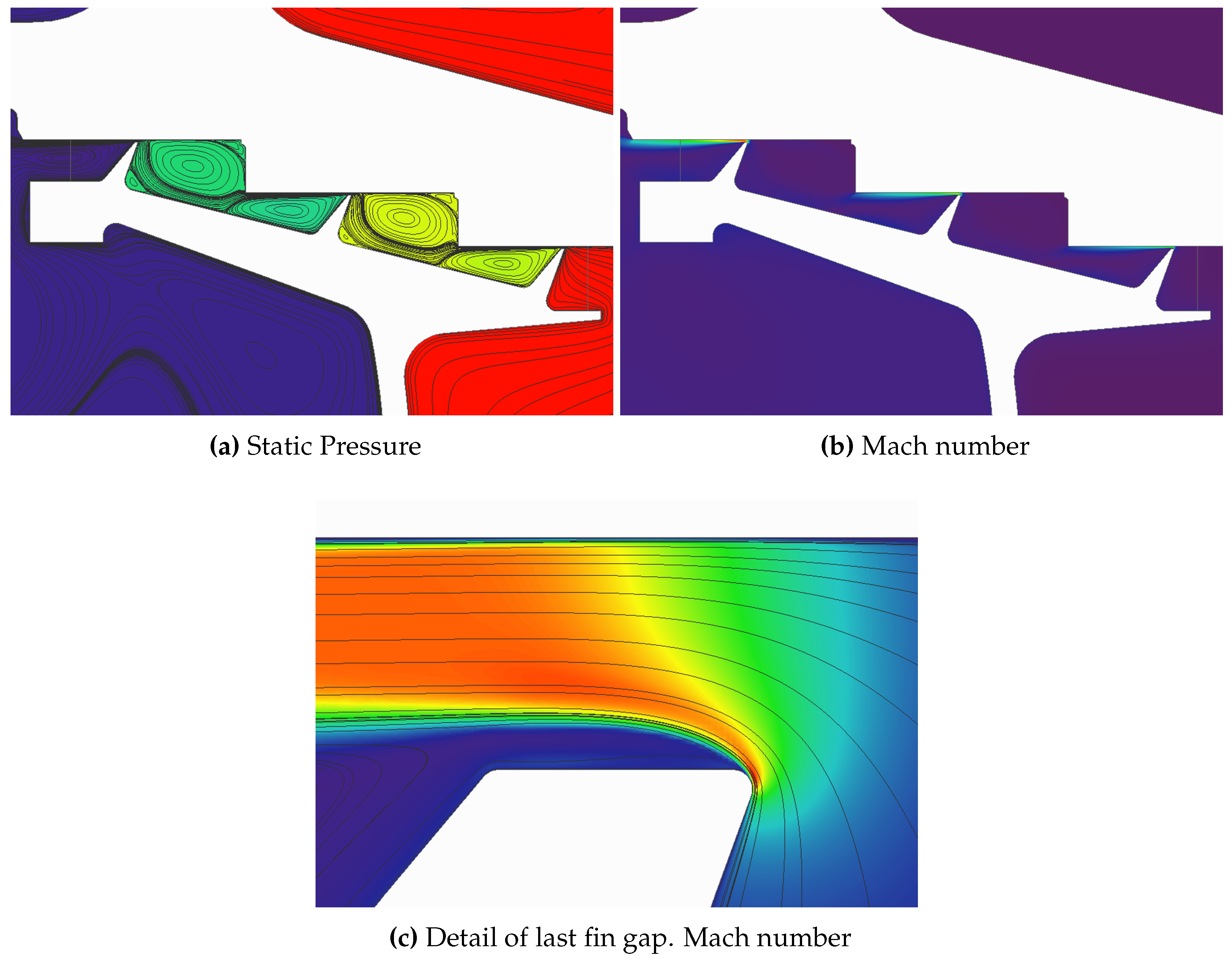
Figure 11.
Unsteady flow field at inter-fin cavities for the baseline geometry, simplified domain and nominal (0.3 mm) gaps. Operating point: 1500 rpm, ΔP=0.1513 MPa.
Figure 11.
Unsteady flow field at inter-fin cavities for the baseline geometry, simplified domain and nominal (0.3 mm) gaps. Operating point: 1500 rpm, ΔP=0.1513 MPa.
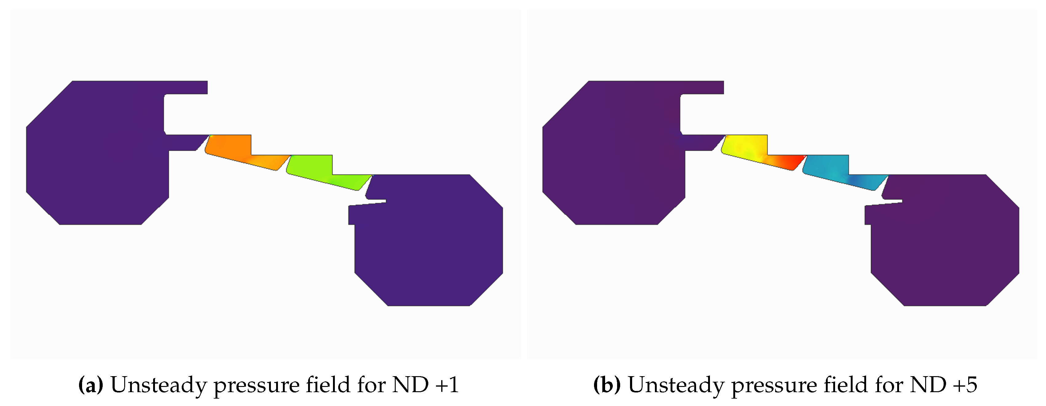
Figure 12.
Baseline geometry experimental SG readings (CTA Campaign).
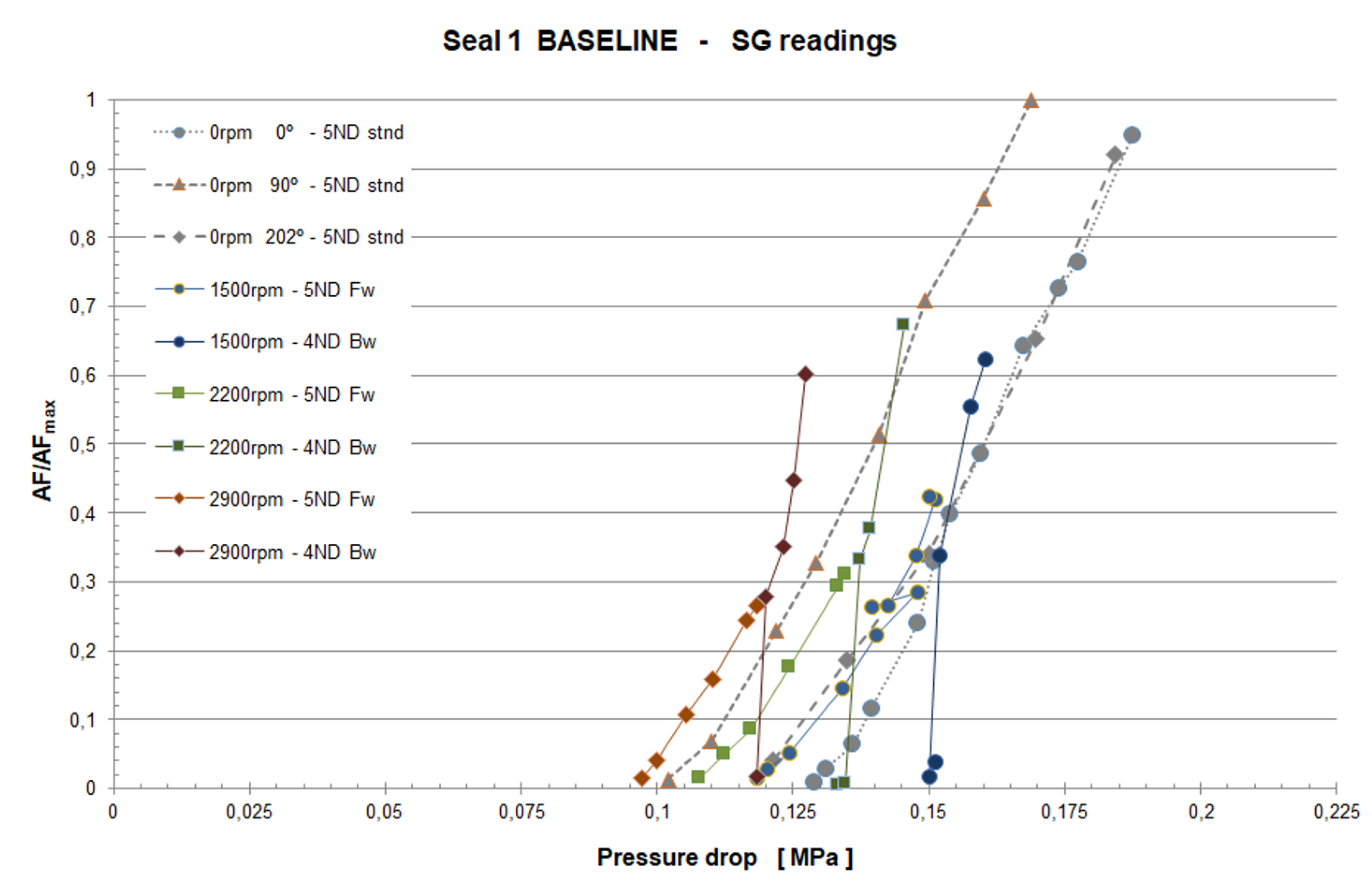
Figure 13.
Two-fin geometry experimental SG readings (CTA Campaign).
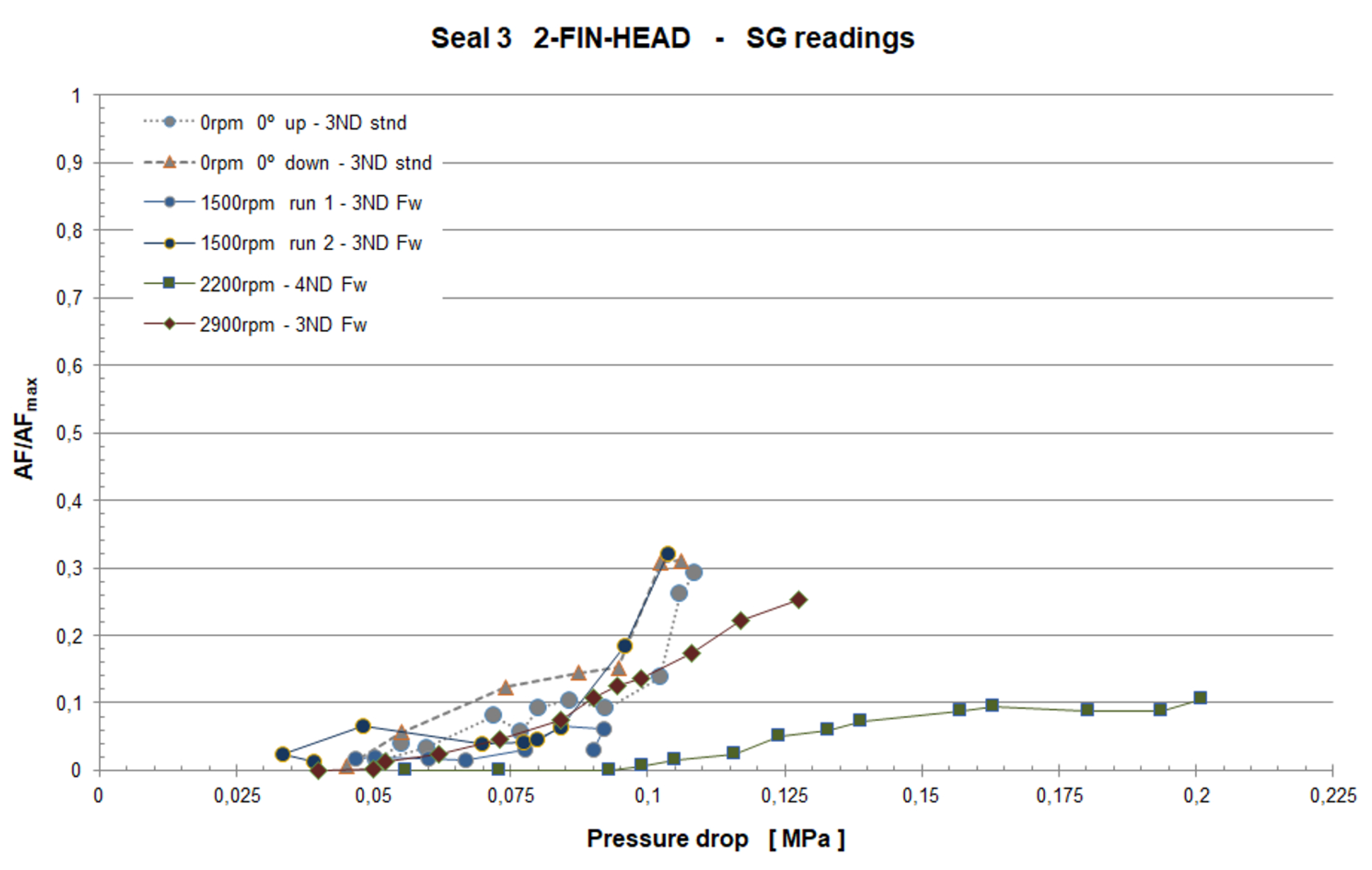
Figure 14.
Example of aerodynamic damping curves for the baseline and two-fin geometries at 1500 rpm. Simulation with nominal gaps and simplified domain.
Figure 14.
Example of aerodynamic damping curves for the baseline and two-fin geometries at 1500 rpm. Simulation with nominal gaps and simplified domain.
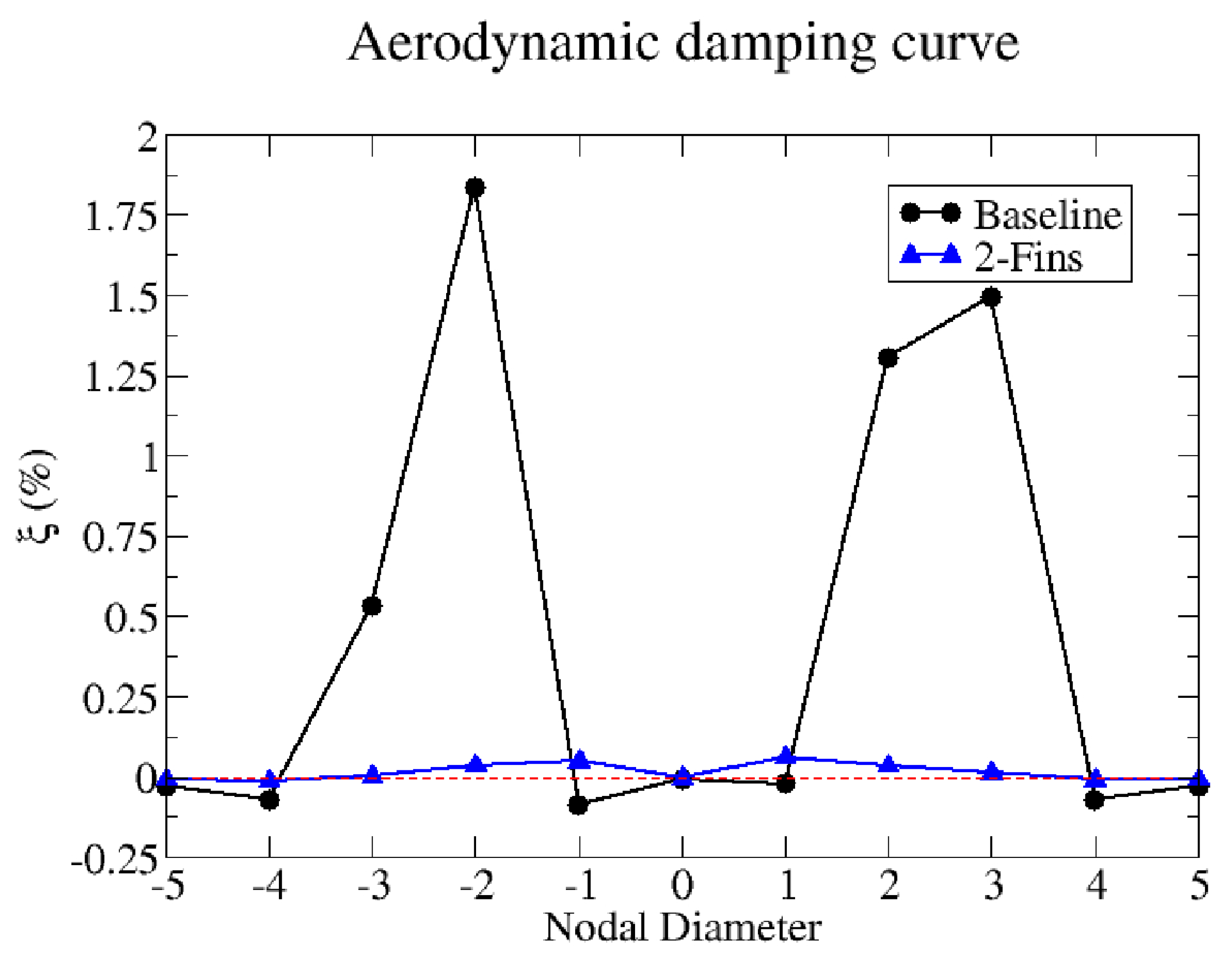
Figure 15.
Unsteady pressure in external cavities for ND 0.
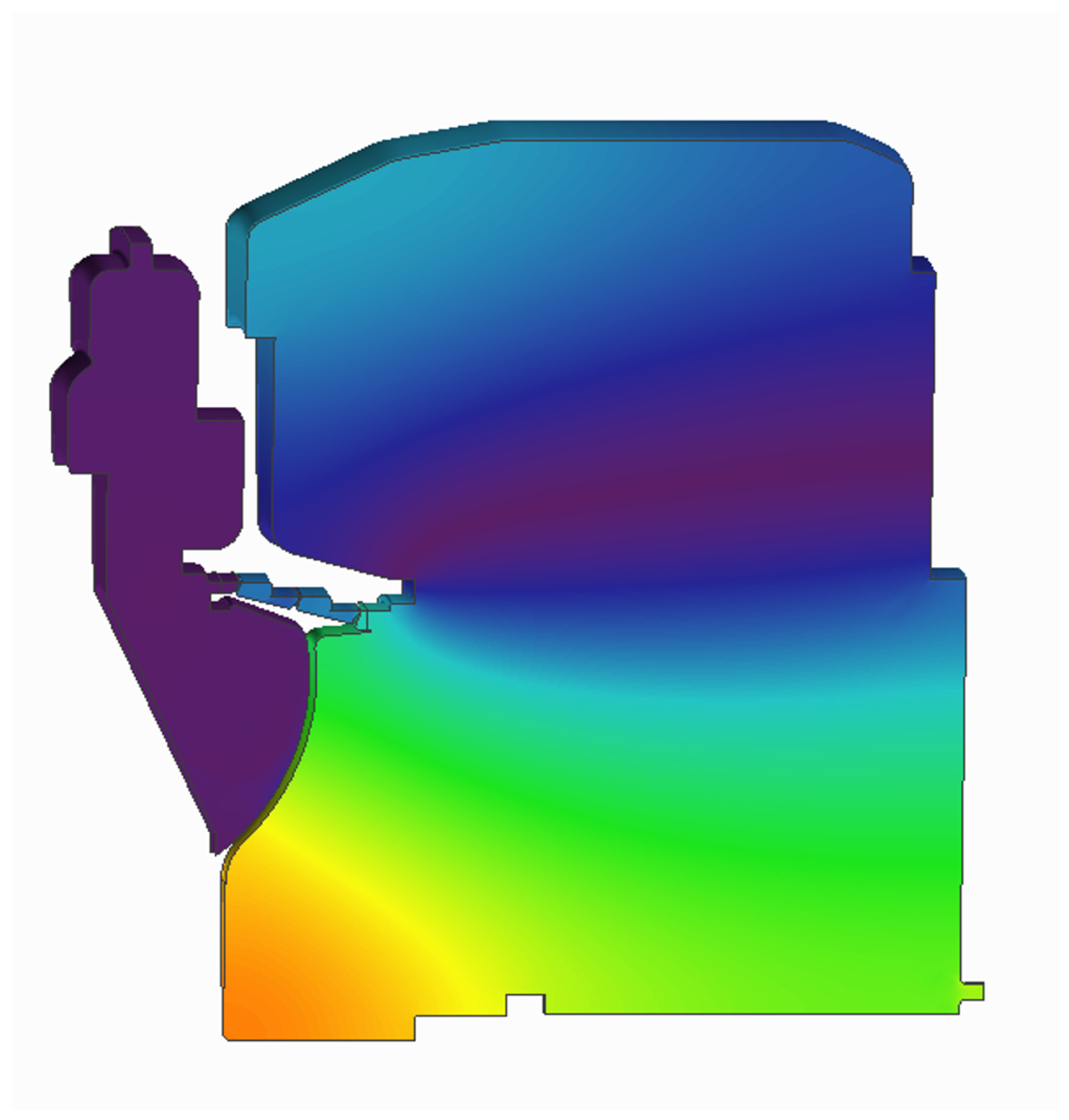
Table 1.
CFD grids characteristics.
| Domain | Sector degrees | Meridional Planes | Nodes per plane |
|---|---|---|---|
| Simplified | 18 | 11 | 23000 |
| Extended | 18 | 19 | 125000 |
Table 3.
Discrepancies between CFD steady simulations (adjusted gaps) and experimental data.
| Configuration | Ω (r.p.m.) | ΔP (MPa) | Err. | Err. | Err. |
|---|---|---|---|---|---|
| Baseline | 0 | 0.1674 | -1.58 % | 0.42 % | -2.44 % |
| 1500 | 0.1513 | -1.89 % | 0.16 % | -2.23 % | |
| 2200 | 0.1392 | -0.32 % | -0.03 % | -2.40 % | |
| 2900 | 0.1251 | 2.37 % | -0.61 % | -2.98 % | |
| 2 Fins | 0 | 0.1059 | -0.10 % | 0.07 % | - |
| 1500 | 0.0968 | -0.37 % | 0.37 % | - | |
| 2200 | 0.1037 | -0.57 % | 0.03 % | - | |
| 2900 | 0.1081 | -0.06 % | 0.08 % | - |
Table 4.
Flutter instabilities from simplified domain simulations. Results with nominal and adjusted gaps.
Table 4.
Flutter instabilities from simplified domain simulations. Results with nominal and adjusted gaps.
 |
Table 5.
Flutter instabilities from full domain simulations with adjusted gaps.
 |
Disclaimer/Publisher’s Note: The statements, opinions and data contained in all publications are solely those of the individual author(s) and contributor(s) and not of MDPI and/or the editor(s). MDPI and/or the editor(s) disclaim responsibility for any injury to people or property resulting from any ideas, methods, instructions or products referred to in the content. |
© 2023 by the authors. Licensee MDPI, Basel, Switzerland. This article is an open access article distributed under the terms and conditions of the Creative Commons Attribution (CC BY) license (http://creativecommons.org/licenses/by/4.0/).
Copyright: This open access article is published under a Creative Commons CC BY 4.0 license, which permit the free download, distribution, and reuse, provided that the author and preprint are cited in any reuse.


