1. Introduction
Permanent Magnet Synchronous Motor (PMSM) drives find extensive use in industrial processes owing to their inherently high torque-to-inertia ratio, facilitated by high flux density, compact size, and enhanced dynamic performance [
1,
2,
3,
4]. Discussions often revolve around enhancing the accuracy, stability and robustness of their control methodologies. A widely used industrial control method, such as
field-oriented control of PMSMs, heavily relies on accurate rotor position [
2]. However, the requirement for high-precision sensors comes at a cost, often requiring enclosed housing, which limits their applicability in specialized environments. In demanding conditions involving severe pressure, humidity, temperature, and vibration, traditional mechanical encoders prove inadequate [
5,
6]. Systems called
sensorless present a potential solution by eliminating the necessity for mechanical sensors. This becomes particularly crucial during safety operations following sensor failure, especially in inaccessible environments [
5]. Consequently, significant interest has been directed towards developing sensorless drives, utilizing the inherent behavior of PMSMs as kind of virtual position sensors. In general, the advantages of these drive systems encompass potentially reduced drive costs, fewer integrated parts, smaller size, heightened reliability, and easier maintenance. However, their drawbacks primarily include low load capacity, limited speed accuracy, and instability in generating low-speed ranges [
4,
7].
In recent years, considerable research has focused on flux and shaft position estimation methods for drive systems in both Induction Motors and PMSMs, broadly categorized into two groups: those based on physical phenomena and algorithmic methods, called observers. Reference [
8] outlines a primary method based on physical nonlinear behavior of magnetic circuit in induction motors. Additionally, the injection of high-frequency signals to emulate similar properties has also found utilization [
3,
9]. The second major group involves algorithmic methods. The Electromagnetic Force (EMF) estimator is extensively used to acquire speed and position information, as seen in [
4,
10,
11]. Other proposed computational methods, such as those based on the basic sliding mode observer, are developed in [
12,
13]. Observers based on the Kalman filter (KF) [
14] also find application. For nonlinear systems like PMSMs, Extended Kalman Filter (EKF) based observers are prevalent [
4,
15,
16,
17]. However, due to the inherent unreliability and inaccuracy of the EKF for not smooth and not analytically differentiable nonlinear circuits, an alternative approach using unscented transformation has emerged [
18,
19]. The unscented Kalman Filter (UKF) significantly reduces nonlinearity issues associated with Gaussian noises and truncation errors, making it a viable replacement for EKF [
4,
20].
Model Predictive Control (MPC) stands as an advanced method in complex process control, frequently applied in chemical, pharmaceutical, petrochemical, and vehicle dynamics control systems [
21,
22,
23]. Historically, their computational demands limited applications to slower control cycles. MPC operates on an iterative control concept, leveraging a system model to predict future states within finite horizons, considering constraints and dynamic behaviors with necessity of knowledge of full system state - measured or estimated.. Notably, it has found successful applications in electromechanical systems in [
24,
25] and robotics in [
26]. Recent literature as [
27] introduces MPC solutions as for electric drive control, including current control in Induction machines [
16,
28,
29], and even in the domain of brushless DC Motors with separate speed and current control [
30]. Cascade MPC is commonly employed for speed control, enabling torque limitation to the maximum value while ensuring optimal dynamic performance [
27,
29]. Solutions proposed in [
31,
32] advocate using EKF as a state observer with a full state vector for MPC.
Based on previous author experience in sensorless control with
PID controllers [
4,
33,
34], extensive research has been dedicated to control systems to achieve higher-precision MPC sensorless control of PMSMs based on UKF obtained state.
2. Methods
A proposed cascade MPC is often used for speed control, which allows to limit the torque (currents) to the maximum admissible value, while providing optimal dynamic performance [
27]. An opposite approach is to introduce full Model Predictive Control. Controlled values are estimated by the unscented Kalman filter.
2.1. Proposed Sensorless Control Scheme
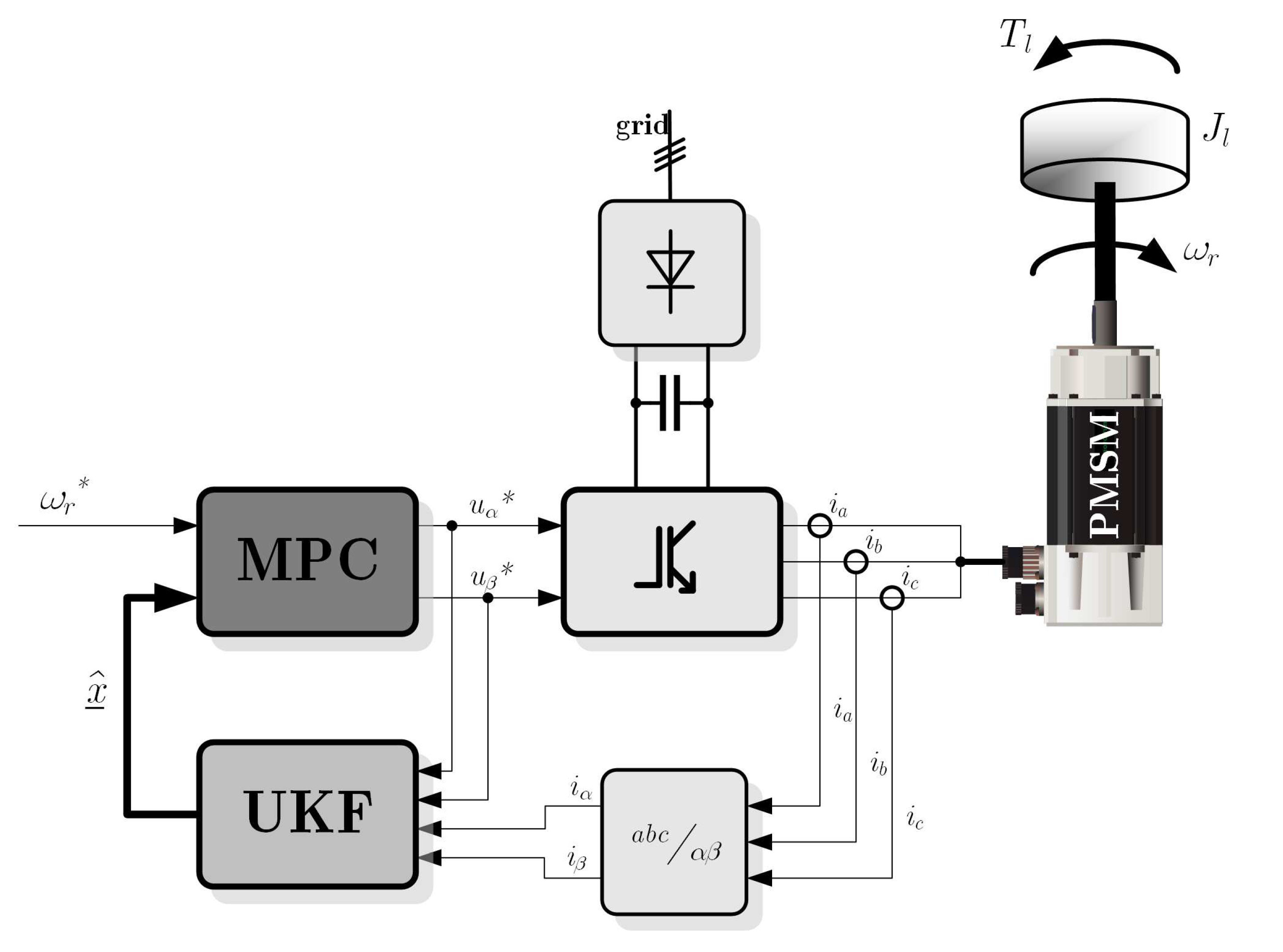
A block diagram of the proposed sensorless scheme is shown in
Figure 1. Signals for UKF, like stator currents (measured by sensors) and stator voltages, are defined as desired by MPC. For the values of natural output (currents, speed and position) only the desired speed
was chosen.
The effectiveness of the proposed drive system has been verified in that scheme (
Figure 1).
2.2. Mathematical Model of PMSM for MPC and UKF
The process model plays a decisive role in the controller. In order to predict the future behaviour of a process, we must have a model of how the process behaves. A model is also necessary for the expected signal estimation via the unscented Kalman filter. The chosen model must be able to capture the process dynamics to predict with precision the future outputs based on estimated states.
The mathematical model of PMSM has three main parts: electrical network, electromechanical torque production and the mechanical subsystem [
35]. The stator of PMSM and Induction Motor is similar. The rotor consists of permanent magnets (modern rare-earth magnets with high strength).
During investigations, some simplified assumptions are made: saturation is negligible, inducted electromagnetic force is sinusoidal, eddy currents and hysteresis losses are negligible, no dynamical dependencies in air-gap, no rotor cage. Under these assumptions, the rotor oriented
electrical network equations of PMSM can be described as:
where:
,
are
axis voltages,
,
are
axis currents,
,
are
axis inductances,
is stator resistance and
is magnetic flux produced by permanent magnets placed on the rotor.
The value of the produced electromagnetic torque is given by equation:
where
p is the number of pole pairs, and fraction
stems from frame conversion: perpendicular stator
over rotor
.
Drive dynamics can be described as:
where
is load torque, and
J is the summary moment of inertia of the kinematic chain.
Based on (
3) and (
4) the movement equation is:
Rotor position –
can be described by the derivative equation of rotational speed:
For this work, the true assumption that load torque
is invariable in a narrow interval holds:
The state-space model can be described as a classical discrete state-space model with sample time
:
For the synthesis of the unscented Kalman filter, state vector
was chosen:
with all natural state variables and estimated load torque
. Considering above that system matrix
has a form:
where:
Output matrix
is a rotating matrix – Clark/Parck transformation:
and matrix
:
Speed Model Predictive Control vector
x is simplified into form:
State matrices are simplified respectively. Load torque
is treated as a known disturbance. The appearance of the model of decoupled
axes determines the method of control.
2.3. Unscented Kalman filter
The primary difficulty of non-linear systems estimation is to determine the non-linear function of state, output and probability distribution [
18,
19,
36]. It appears that the non-linear transformation of what is to deviate and
Jacobians counting for an
Extended Kalman filter (EKF) do not determine real covariances. The unscented Kalman filter (UKF) is an improvement over previous algorithms and an entirely novel solution to the estimation theory problem based on
unscented transformation [
18]. It is easier to define and approximate the Gaussian distribution associated with each state vector variable, than using the approximated non-linear function transformation [
18]. The EKF also made it possible to simplify the algorithm by eliminating the need for calculating
Jacobians at each working point. This is based on two assumptions. The first is the determination of the non-linear transform of the function at work, and not in the entire range of probability density distribution function. The second point concerns the search for work in which this density corresponds to the actual decomposition of the non-linear system. This filter, like its classical form, is based on two cycles:
prediction and
correction [
14].
The prediction of UKF can be used independently from the UKF update, in combination with a linear update. In this case, however, the estimation state vector of the value of disturbances is extended. Such a procedure makes it possible to estimate the state vector and its environment (with disturbances).
Based on [
18] the defined augmented estimation vector
can be defined as:
which consists state vector
and expected noise terms
and
, with definition of each covariance:
An important set of
sigma points –
is derived from the augmented state and covariances, where
L is the dimension of the augmented state:
The sigma points
are propagated through the state-space transition function:
The weighted sigma points
are recombined to produce the predicted state
and covariance
:
where the weights
and
for the state and covariance [
37] are given by:
where
,
,
are noise distribution parameters, and
is chosen arbitrarily.
During
correction, the sigma points
are projected through the observation function
:
Based on weights
and
from Equation (
24) and observation matrix
, it is possible to obtain the following output signal:
and also output covariance:
The solution of the classical form of the Kalman filter is adapted in UKF. Correction
depends directly on state covariances
and the innovation of system covariances
, so it is similar to (
27):
where
can be described as:
As in the classical Kalman filter outputs the residuum is:
Correction of state is done by:
The adjusted covariance matrix
is a prediction of
, corrected by weighted values:
The entire algorithm is recurrent – data from the actual step are input data for the next.
2.4. Model Predictive Control
Model Predictive Control is an advanced control scheme, where the control signal is obtained by solving an open-loop optimal multi-variable control problem over a given predictive horizon [
23]. This method is sometimes called
Receding Horizon Control. Optimisation should produce an optimal control sequence with a given cost over the given control and system constraints.
Philosophically, MPC reflects human behaviour in that it selects control actions thought to lead to the best predicted outcome (or output) over a limited horizon. In normal application, one MPC based controller plays the role of the whole system controller, with full knowledge of system behaviour and all computed control signals.
2.4.1. Foundation
One advantage of predictive control is that concepts are very simple and intuitive. As the controller has to predict the future behaviour of the system, the core of MPC is the model of the system presented above. Control law strictly depends on predicted behaviour.
In the literature, MPC is formulated in the state-space approach. Let the model of the plant to be controlled be described by the linear discrete-time state-space equations:
where:
are vectors of state, output and input respectively. The cost function
that has to be minimised in receding horizon
N, generally takes the quadratic form:
When we assume an
N step prediction, system output behaviour can be determined in the following
N steps:
written most simply:
where:
Based on the above and the definition of optimisation cost in (
36), they can be compared with the desired state of the system:
The optimiser is a crucial part of the strategy, as it provides the control. The combination of (
36) and (
41) can be solved by the
quadratic programming (QP) problem as:
for minimising the value of control signal
in each future predicted state
N. The reference speed signal was introduced into the
vector. Since the problem depends on current state
, the implementation of MPC requires the on-line solution of a
QP at each time step
k.
2.4.2. Constraints
Based on finding the min of cost function (
42), which has a form:
it can be possible to introduce some constraints which rule:
Considering maximum voltage:
and predicted state constraints:
quadratic programming (QP) yield optimised results.
This paper focused specifically on the axis current ( and ) limitation and maximum supply voltage ( and ). Other limitations seem not to apply here.
The presented optimization can now be recognized and simplified to solve
QP problem with linear inequality constraints [
38]. The problem is convex, but due to the constraints, it is not possible to write the solution on closed form. Rather iterative algorithms have to be employed. Concerning performance, few methods have advantages and disadvantages when applied to MPC, and during this work decided to
active set algorithm with iterative state values [
39].
3. Results
After numerous simulation studies the experimental verification of the proposed control method, existing for other research laboratory setup has been used [
40]. An implementation in real astronomy telescope mount systems is investigated [
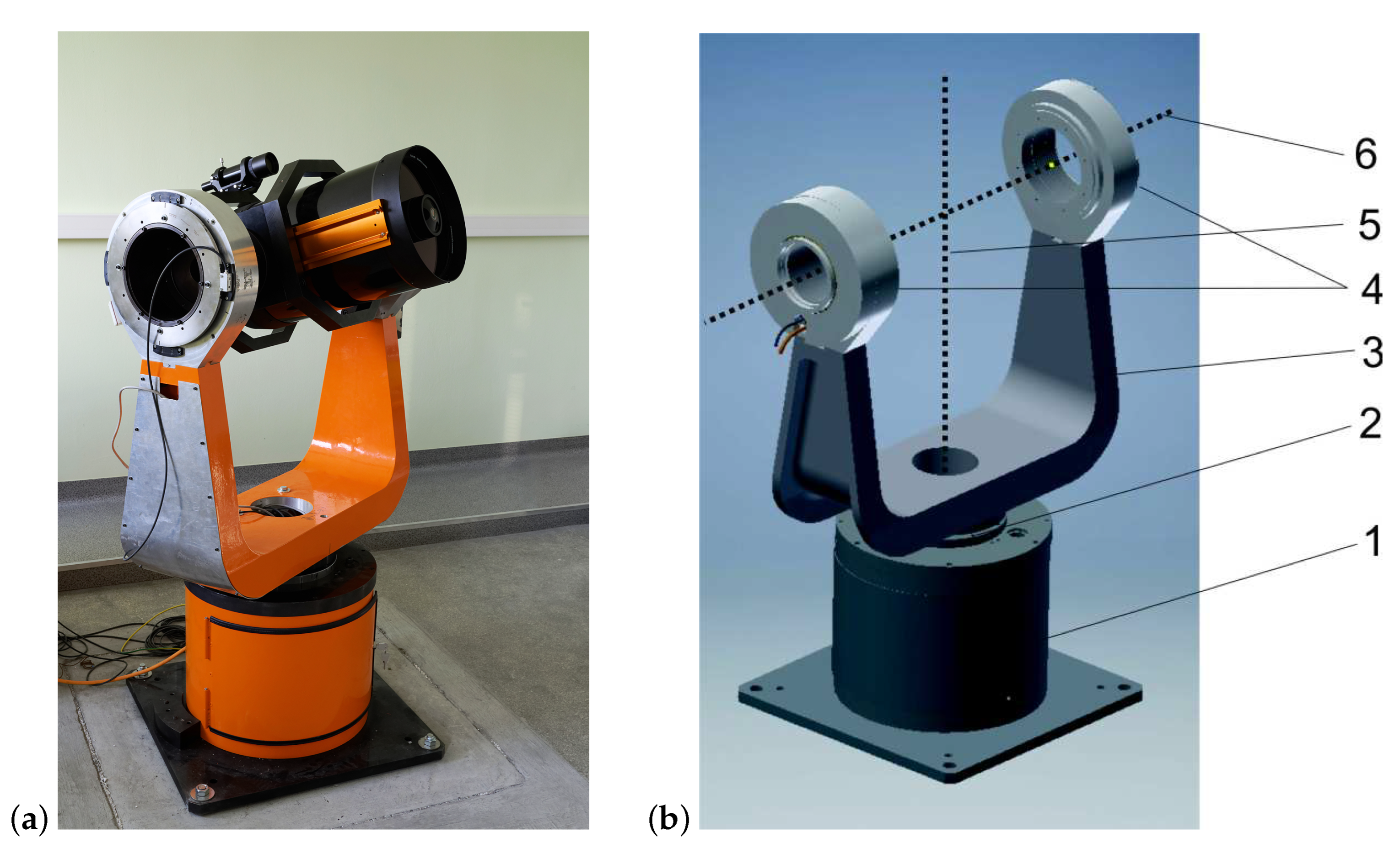
40]. The base axis of laboratory stand, presented in
Figure 2 consists of the surface mounted magnets synchronous motor, supplied from a three-phase IGBT power inverter controlled by
Texas Instruments Sitara AM335x and
Altera FPGA Cyclone IV board . The developed MPC algorithm has been widely simulated in different conditions before implementation. Bellow real results are only partly presented to demonstrate its operation. Some advantages of sensorless UKF with coordinated PI current and speed controllers were considered during the tuning of the observer. From the collection of sets, one conditional example was chosen for the number of predicted states
. Equation (
42) was extended into:
which is:
with maximum weight equal to 30 for speed
control based on numerous simulation studies. An important point of that investigation was setting the maximum value of control signal
V, and the maximum value of currents (state vector
elements):
A,
A in a circular shape.
The state observer based on UKF was tuned as in the classical coordinate system [
41], with any extra tuning not focused on any control quality criteria. This proved to be an important indication of the possibility of the MCP to control based on the estimated state, and sensorless control procedure build up.
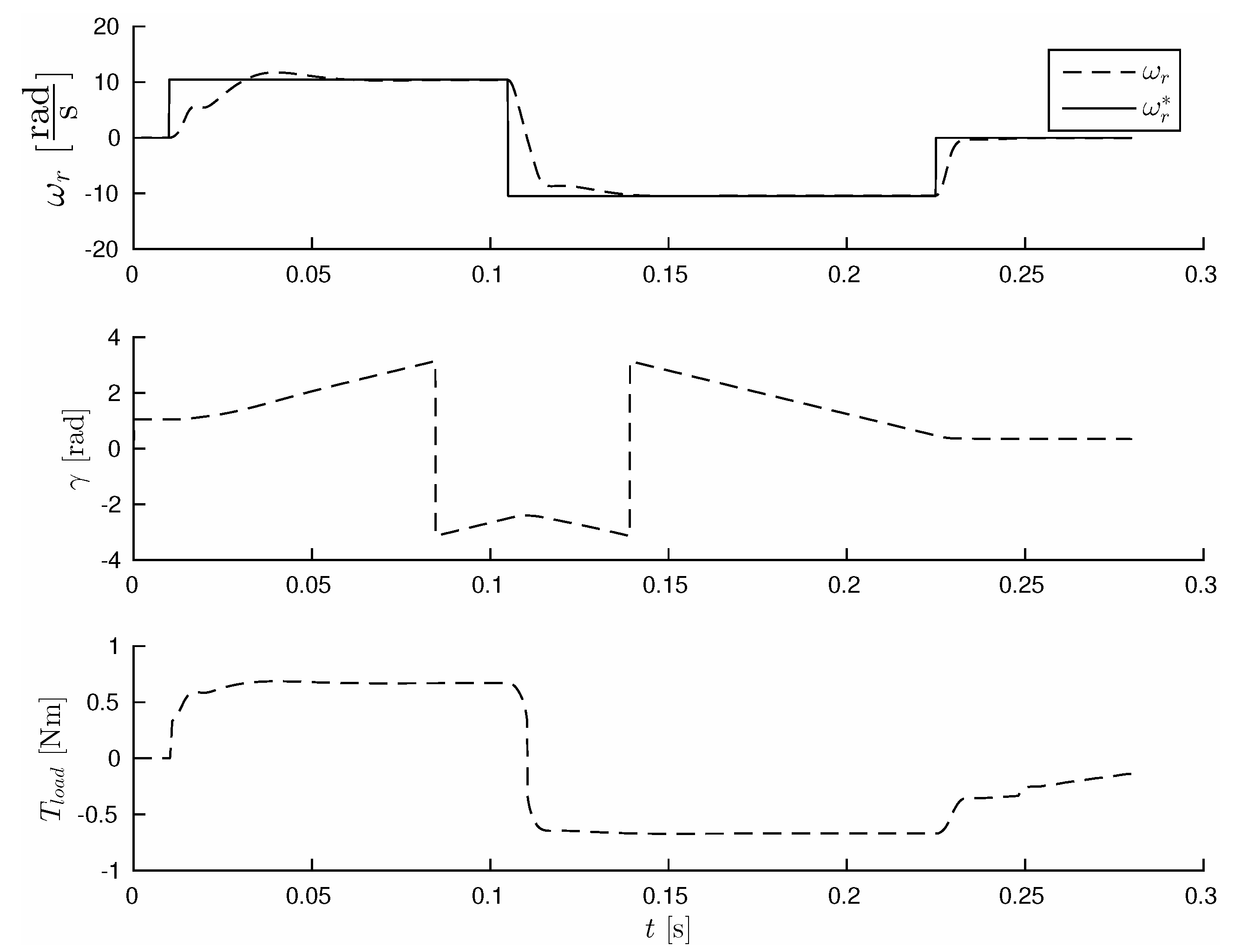
The first part of this investigation was focused on controlled system behaviour by reference speed change and the possibilities to obtain initial position after the algorithm was stated.
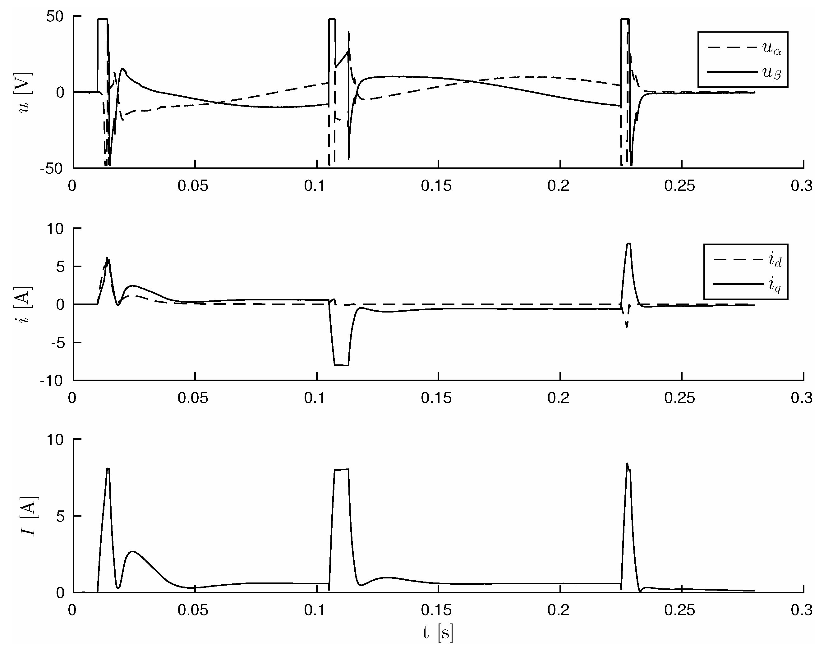
Figure 3 shows the system’s response to the rapid change of speed
. Additional interesting signals (including actual control voltages
) are presented in
Figure 4.
An initial point can be found by applying any voltages to drive based on the first predictive step. The unscented Kalman filter in that form can find the proper actual position of after a few steps. This process does not interfere with the MPC algorithm.
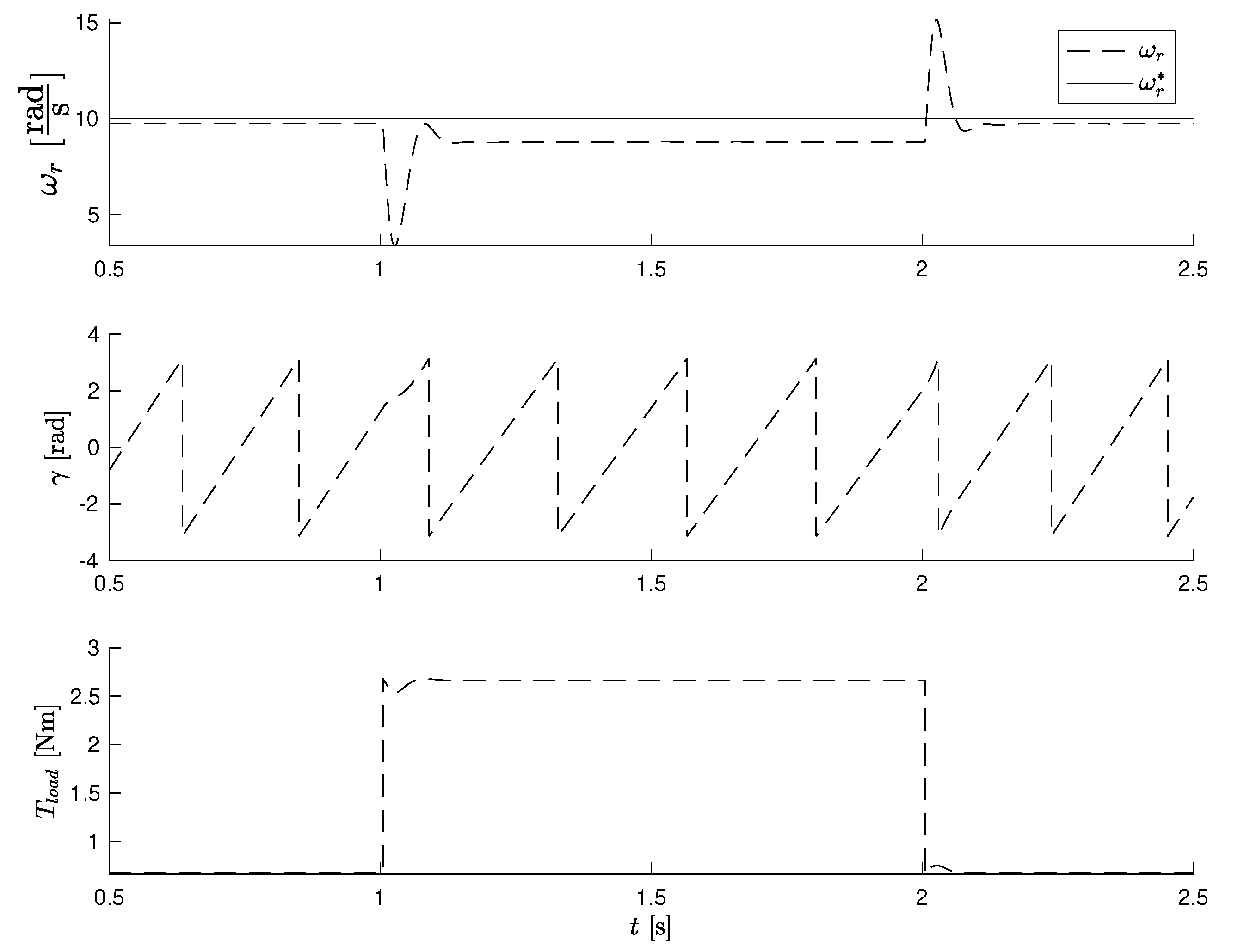
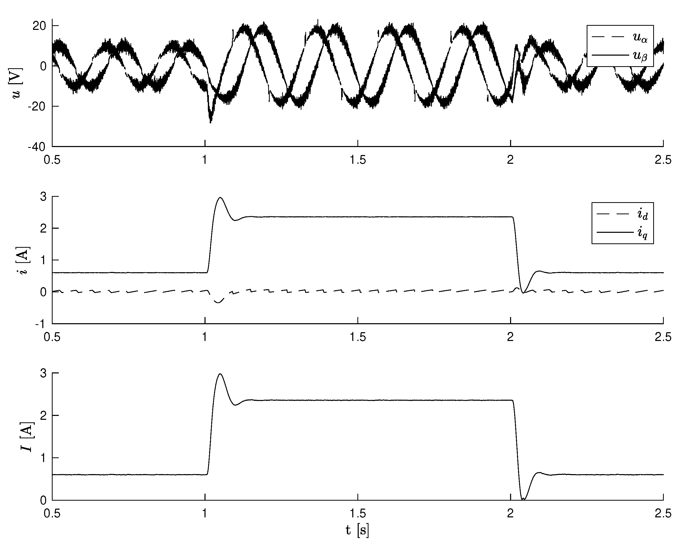
Additional investigation concerns the external load torque disturbance, kick type additional force. Properties are presented in
Figure 5. Fast dynamic reaction can be observed but a steady state error remains. Actual control voltages
and motor currents
,
with modulus
I are presented in
Figure 6.
The proposed control algorithms are able to respond quickly to significant disturbance. A fixed error in controlled speed appeared. In some cases, where speed is at a standstill, some systematic fixed errors are encountered and source can be found in static disturbance - rough friction. Based on the observed values (e.g., ) from UKF, it will be possible to cancel all these errors, which would be the subject of further research.
4. Conclusions
The main contribution of this paper is the introduction of a new original sensorless highly dynamic performance control scheme for permanent magnet drives based on
MPC. It can be observed that this controller has a good dynamic performance in all working points, even for zero speed. It is worth noticing that the
model for control signal prediction determines a type of control similar to
vector control [
2]. The advantages of the proposed
MPC algorithm in high dynamic systems have been shown. The proposed algorithm is strongly recommended for control in rapid speed change circumstances.
The paper shows successful way of design of the control system MPC with unscented Kalman filter. Currently, continued development work is planed in field of reducing control error and dynamical behavior as well as the implementation of proposed algorithm in industrial drive system.
Funding
This research received no external funding
Acknowledgments
In this section you can acknowledge any support given which is not covered by the author contribution or funding sections. This may include administrative and technical support, or donations in kind (e.g., materials used for experiments).
Conflicts of Interest
The author declare no conflict of interest.
Abbreviations
The following abbreviations are used in this manuscript:
| PMSM |
Permament Magnet Synchronous Motor |
| MPC |
Model Predictive Control |
| UKF |
Unscented Kalman Filter |
References
- Pellegrino, G.; Vagati, A.; Guglielmi, P.; Boazzo, B. Performance Comparison Between Surface-Mounted and Interior PM Motor Drives for Electric Vehicle Application. IEEE Transactions on Industrial Electronics 2012, 59, 803–811. [Google Scholar] [CrossRef]
- Vas, P. Vector Control of AC Machines; Monographs in Electrical and Electronic Engineering; Oxford University Press, 1990. [Google Scholar]
- Wang, G.; Valla, M.; Solsona, J. Position Sensorless Permanent Magnet Synchronous Machine Drives—A Review. IEEE Transactions on Industrial Electronics 2020, 67, 5830–5842. [Google Scholar] [CrossRef]
- Urbanski, K.; Janiszewski, D. Sensorless Control of the Permanent Magnet Synchronous Motor. Sensors 2019, 19. [Google Scholar] [CrossRef]
- Batzel, T.; Lee, K. Electric propulsion with the sensorless permanent magnet synchronous motor: Model and approach. IEEE Transactions on Energy Conversion 2005, 20, 818–825. [Google Scholar] [CrossRef]
- Briz, F.; Degner, M.W. Rotor Position Estimation. IEEE Industrial Electronics Magazine 2011, 5, 24–36. [Google Scholar] [CrossRef]
- Vas, P. Sensorless Vector and Direct Torque Control; Monographs in Electrical and Electronic Engineering number 42, Oxford University Press, 1998.
- Schroedl, M. An improved position estimator for sensorless controlled permanent magnet synchronous motors. 4th European Conference on power Electronics and Applications – EPE ’91, Proceedings of 1991, 3, 418–423. [Google Scholar]
- Wang, S.; Yang, K.; Chen, K. An Improved Position-Sensorless Control Method at Low Speed for PMSM Based on High-Frequency Signal Injection into a Rotating Reference Frame. IEEE Access 2019, 7, 86510–86521. [Google Scholar] [CrossRef]
- Urbanski, K. Estimation of Back EMF for PMSM at Low Speed Range. MM (Modern Machinery) Science Journal 2015, 564–569. [Google Scholar] [CrossRef]
- He, C.; Xu, S.; Yan, B.; Wang, Z.; Wang, M. A Fixed-Point Position Observation Algorithm and System-on-Chip Design Suitable for Sensorless Control of High-Speed Permanent Magnet Synchronous Motor. Electronics 2023, 12. [Google Scholar] [CrossRef]
- Woldegiorgis, A.T.; Ge, X.; Li, S.; Hassan, M. Extended Sliding Mode Disturbance Observer-Based Sensorless Control of IPMSM for Medium and High-Speed Range Considering Railway Application. IEEE Access 2019, 7, 175302–175312. [Google Scholar] [CrossRef]
- Ma, Z.; Zhang, X. FPGA Implementation of Sensorless Sliding Mode Observer With a Novel Rotation Direction Detection for PMSM Drives. IEEE Access 2018, 6, 55528–55536. [Google Scholar] [CrossRef]
- Kalman, R.E. A New Approach to Linear Filtering and Prediction Problems. Transactions of the ASME–Journal of Basic Engineering 1960, 82, 35–45. [Google Scholar] [CrossRef]
- Taheri, A.; Ren, H.; Holakooie, M.H. Sensorless Loss Model Control of the Six-Phase Induction Motor in All Speed Range by Extended Kalman Filter. IEEE Access 2020, 8, 118741–118750. [Google Scholar] [CrossRef]
- Wang, Y.; Yu, H.; Che, Z.; Wang, Y.; Zeng, C. Extended State Observer-Based Predictive Speed Control for Permanent Magnet Linear Synchronous Motor. Processes 2019, 7. [Google Scholar] [CrossRef]
- Dilys, J.; Stankevič, V.; Łuksza, K. Implementation of Extended Kalman Filter with Optimized Execution Time for Sensorless Control of a PMSM Using ARM Cortex-M3 Microcontroller. Energies 2021, 14. [Google Scholar] [CrossRef]
- Julier, S.J.; Uhlmann, J.K. Unscented filtering and nonlinear estimation. Proceedings of the IEEE 2004, 92, 401–422. [Google Scholar] [CrossRef]
- Yin, L.; Deng, Z.; Huo, B.; Xia, Y.; Li, C. Robust Derivative Unscented Kalman Filter Under Non-Gaussian Noise. IEEE Access 2018, 6, 33129–33136. [Google Scholar] [CrossRef]
- Rosafalco, L.; Eftekhar Azam, S.; Manzoni, A.; Corigliano, A.; Mariani, S. Unscented Kalman Filter Empowered by Bayesian Model Evidence for System Identification in Structural Dynamics. Computer Sciences & Mathematics Forum 2022, 2. [Google Scholar] [CrossRef]
- Grüne, L.; Pannek, J. , 2011; pp. 43–66. https://doi.org/10.1007/978-0-85729-501-9_3.Control. In Nonlinear Model Predictive Control: Theory and Algorithms; Springer London: London, 2011; pp. 43–66. [Google Scholar] [CrossRef]
- Corriou, J.P. , Process Control: Theory and Applications; Springer London: London, 2004. [Google Scholar] [CrossRef]
- García, C.E.; Prett, D.M.; Morari, M. Model predictive control: Theory and practice–A survey. Automatica 1989, 25, 335–348. [Google Scholar] [CrossRef]
- Comarella, B.V.; Carletti, D.; Yahyaoui, I.; Encarnação, L.F. Theoretical and Experimental Comparative Analysis of Finite Control Set Model Predictive Control Strategies. Electronics 2023, 12. [Google Scholar] [CrossRef]
- Morel, F.; Lin-Shi, X.; Retif, J.M.; Allard, B.; Buttay, C. A Comparative Study of Predictive Current Control Schemes for a Permanent-Magnet Synchronous Machine Drive. IEEE Transactions on Industrial Electronics 2009, 56, 2715–2728. [Google Scholar] [CrossRef]
- Zhang, A.; Lin, Z.; Wang, B.; Han, Z. Nonlinear Model Predictive Control of Single-Link Flexible-Joint Robot Using Recurrent Neural Network and Differential Evolution Optimization. Electronics 2021, 10. [Google Scholar] [CrossRef]
- Cortes, P.; Kazmierkowski, M.P.; Kennel, R.M.; Quevedo, D.E.; Rodriguez, J. Predictive Control in Power Electronics and Drives. IEEE Transactions on Industrial Electronics 2008, 55, 4312–4324. [Google Scholar] [CrossRef]
- Rojas, C.A.; Yuz, J.I.; Silva, C.A.; Rodriguez, J. Comments on “Predictive Torque Control of Induction Machines Based on State-Space Models ”. IEEE Transactions on Industrial Electronics 2014, 61, 1635–1638. [Google Scholar] [CrossRef]
- Cataldo, P.; Jara, W.; Riedemann, J.; Pesce, C.; Andrade, I.; Pena, R. A Predictive Current Control Strategy for a Medium-Voltage Open-End Winding Machine Drive. Electronics 2023, 12. [Google Scholar] [CrossRef]
- Darba, A.; De Belie, F.; D’haese, P.; Melkebeek, J.A. Improved Dynamic Behavior in BLDC Drives Using Model Predictive Speed and Current Control. IEEE Transactions on Industrial Electronics 2016, 63, 728–740. [Google Scholar] [CrossRef]
- Li, J.; Zhang, L.; Niu, Y.; Ren, H. Model predictive control for extended Kalman filter based speed sensorless induction motor drives. In Proceedings of the 2016 IEEE Applied Power Electronics Conference and Exposition (APEC), March 2016; pp. 2770–2775. [Google Scholar] [CrossRef]
- Soliman, A.I.; Farhan, A.; Abdelrahem, M.; Kennel, R. Enhanced Sensorless Model Predictive Control of Induction Motor Based on Extended Kalman Filter. In Proceedings of the 2019 IEEE Conference on Power Electronics and Renewable Energy (CPERE), Oct 2019; pp. 309–313. [Google Scholar] [CrossRef]
- Janiszewski, D. Extended Kalman Filter Based Speed Sensorless PMSM Control with Load Reconstruction. In Proceedings of the Proc. IECON 2006 - 32nd Annual Conf. IEEE Industrial Electronics; 2006; pp. 1465–1468. [Google Scholar] [CrossRef]
- Janiszewski, D. Disturbance estimation for sensorless PMSM drive with Unscented Kalman Filter. In Proceedings of the Proc. 12th IEEE Int Advanced Motion Control (AMC) Workshop; 2012; pp. 1–7. [Google Scholar] [CrossRef]
- Pillay, P.; Krishnan, R. Modeling, simulation, and analysis of permanent-magnet motor drives. I. The permanent-magnet synchronous motor drive. IEEE Transactions on Industry Applications 1989, 25, 265–273. [Google Scholar] [CrossRef]
- Onat, A. A Novel and Computationally Efficient Joint Unscented Kalman Filtering Scheme for Parameter Estimation of a Class of Nonlinear Systems. IEEE Access 2019, 7, 31634–31655. [Google Scholar] [CrossRef]
- Wan, E.A.; Van Der Merwe, R. The unscented Kalman filter for nonlinear estimation. In Proceedings of the Proc. and Control Symp Adaptive Systems for Signal Processing, Communications 2000. AS-SPCC. The IEEE 2000, 2000, pp. 153–158. [Google Scholar] [CrossRef]
- Gould, N.; Toint, P.L. Preprocessing for quadratic programming. Mathematical Programming 2004, 100, 95–132. [Google Scholar] [CrossRef]
- Bartlett, R.; Wachter, A.; Biegler, L. Active set vs. interior point strategies for model predictive control. In Proceedings of the Proceedings of the 2000 American Control Conference.; pp. 0036334200064229–42336. [CrossRef]
- Kozlowski, K.; Pazderski, D.; Krysiak, B.; Jedwabny, T.; Piasek, J.; Kozlowski, S.; Brock, S.; Janiszewski, D.; Nowopolski, K. High Precision Automated Astronomical Mount. In Proceedings of the Automation 2019; Szewczyk, R.; Zieliński, C.; Kaliczyńska, M., Eds., Cham; 2020; pp. 299–315. [Google Scholar] [CrossRef]
- Janiszewski, D. Load torque estimation in sensorless PMSM drive using Unscented Kalman Filter. In Proceedings of the Industrial Electronics (ISIE), june 2011, 2011 IEEE International Symposium on; pp. 643–648. [Google Scholar] [CrossRef]
|
Disclaimer/Publisher’s Note: The statements, opinions and data contained in all publications are solely those of the individual author(s) and contributor(s) and not of MDPI and/or the editor(s). MDPI and/or the editor(s) disclaim responsibility for any injury to people or property resulting from any ideas, methods, instructions or products referred to in the content. |
© 2023 by the authors. Licensee MDPI, Basel, Switzerland. This article is an open access article distributed under the terms and conditions of the Creative Commons Attribution (CC BY) license (http://creativecommons.org/licenses/by/4.0/).
