Submitted:
22 November 2023
Posted:
23 November 2023
You are already at the latest version
Abstract
Categorical data analysis of 2 x 2 contingency tables is extremely common, not least because they provide odds and risk ratio statistics in medical research. The χ2 test is most often used, although some researchers use the likelihood ratio test (LRT). Does it matter which test is used? This paper argues that the LRT rather than the χ2 test should be used when we are interested in testing whether two variables are independent, as is typically the case. In contrast, the χ2 test should be reserved for where the data appear to match too closely a particular hypothesis (e.g. the null hypothesis), as may occur in the investigation of data integrity. Finally, it is argued that the evidential approach provides a consistent and coherent way in which tests can be made for each of these situations.
Keywords:
2 x 2 table
; χ2 test
; likelihood ratio test
; G-test
; likelihood
; odds ratio
; data integrity
; too good to be true
1. Introduction
CHUCK: Well then there’s nothing more to talk about! I will beat this. Ergo, a falsis principiis proficisci. Meaning? (gestures to Saul)
SAUL: That’s the one about false principles, but it’s not…
CHUCK: You proceed from false principles. Your argument is built on quicksand, therefore it collapses.
Better Call Saul
The χ2 distribution is used to test categorical data. The statistic can be calculated from a 2 × 2 table directly using Pearson’s criterion (Pearson 1900)
For i columns and j rows, where we denote the observed count in the ith column and jth row as Oij and the expected value in the ith column and jth row as Eij. The expected values are typically calculated from the marginal totals (usually the null model is that of independence) or according to a specified model (such as one suggested a priori by Mendelian inheritance). The distribution has (i – 1) x (j – 1) = 1 degree of freedom (df). For our purposes, a model represents a means by which data may be produced or predicted. The null model for independence, for example, would predict that the cell values
The log likelihood ratio for two models given the data is given by
Here S represents the term support, which was first defined by Harold Jeffreys as the logarithm of the likelihood ratio for one hypothesis versus another (Jeffreys 1936). This scale represents the relative evidence and ranges from −∞ to +∞, with zero indicating no evidence either way. This is used in the likelihood approach (Goodman and Royall 1988; Edwards 1992; Cahusac 2020).
approximates to the χ2 distribution (Wilks 1938)
This is the form of the likelihood ratio test (LRT, also known as the G-test (Woolf 1957)). There are several advantages of using the LRT over the χ2 test. Better performance when expected numbers are small (Cochran 1936; Fisher 1950), and better theoretical grounding (Fisher 1922; Neyman and Pearson 1928). The LRT has the highest power among other competing tests according to the Neyman-Pearson lemma (Neyman, Pearson, and Pearson 1933). It avoids the χ2 test restriction that expected values should not be less than 5. The LRT is also computationally easier to calculate (Sokal and Rohlf 2009). An important advantage of using the likelihood ratio (Equation (2)) is that sub-tables within a large dimensional table can be independently analyzed, and that components from the sub-tables sum precisely, unlike a χ2 analysis (Agresti 2013). There is general agreement that exact tests are preferable for small samples (Agresti 2013), for example Fisher’s exact test.
For the goodness of fit test where there is single dimension of classification, Fisher (Fisher 1922) (P 357) (and noted by Woolf (Woolf 1957)) gave the expansion for support
where k is the number of categories. The leading term in the expansion is of course half Pearson’s criterion. When the discrepancy between observed and expected relative to expected is small across all categories then
Naturally this extends to the addition of a second dimension in a contingency table.
The 2 × 2 contingency table is commonly encountered in research. For example, it is used in randomized controlled trials where patients are given either treatment or placebo, and the outcome is either healthy or diseased. The design gives rise to risk ratios (relative risk) and odds ratios, which are particularly useful in medical research (Armitage, Berry, and Matthews 2002). In such a table the expected frequencies are typically those representing the null model: that the two proportions from the two rows (or columns) are equal. For the odds ratio we have a 2 × 2 table that arises in a treatment/medical setting.
| Outcome | ||||
| + | − | |||
| Factor | + | a | c | a + c |
| − | b | d | b + d | |
| a + b | c + d | N | ||
Here the null hypothesis is that the two row proportions and are equal
Based upon columns rather than rows would produce the same null model. The expected frequencies can be determined from the marginal totals. The degree of mismatch between observed and expected gives us the so-called test of association or independence.
In this model a statistical test can test two independent parameters. One parameter concerns whether the proportions are equal to each other. The second concerns whether the variance of the frequencies obviously differs (either higher or lower) from sampling variability. Reduced variance is apparent when a smaller X2 statistic is obtained by an analysis. There has been considerable confusion over the meaning of small X2 statistics in categorical data analysis (Stuart 1954; Edwards 1986a). These tests concern the interaction between the two variables (e.g. treatment and outcome). In addition, tests can be made on the equality of the marginal totals (main effects), although these are usually of little or no interest.
The choice of statistical test should depend upon which model parameter is being tested. If a test of proportion equality is required (the typical situation) then the LRT is appropriate. If a test of variance is required (e.g. the data are too good to be true) then the χ2 test should be used. Both tests exploit the χ2 distribution to calculate p values for statistical significance.
2. LRT Statistic versus χ2 Test Statistic
Use of the LRT to test proportions is non-controversial and is accepted as an appropriate way to test proportions. The test is based upon the likelihood of the data under a specific hypothesis (usually the null) relative to maximum likelihood estimates. Edwards (P 191) gives the derivation of equation (2) for the log likelihood ratio from first principles (Edwards 1992). As such it represents a test of two binomial proportions. It does not test the overall model variance. If the observed frequencies exactly matched the expected frequencies then S = 0, indicating no evidence of a difference from the null hypothesis.
The X2 statistic has been used to assess the variance of the model (Cochran 1936), specifically of Mendel’s results of plant hybridization experiments (Fisher 1936; Edwards 1986b) (although Edwards used X rather than X2, which had the advantage of preserving the direction of effect). We can start from first principles and consider the simpler binomial situation (Edwards 1986b). If µ is fixed and part of the model, and alternative hypotheses concern different values for σ2, then all the information we need is given by the X2 statistic with 1 df
This is due to the following. For binomial events µ = np, where n is the number of events in the sample and p is the probability of an event occurring. Hence σ2 = npq, where q = 1 – p. Specifying a as the observed number of successes, and b = n – a will be the number of failures. Thus, a and b are the observed numbers in a binomial trial. Each approximates to a normal distribution, which improves as sample size increases. Our expected numbers are np and nq respectively, since
Each of these last two terms representing the successes and failures respectively, which is
Moreover, the expected variance is the expected value of the denominator in equation (5), and in its binomial form . Knowing σ2 = npq means that, by definition, the expectation of the sum of the two terms for successes and failures will be 1. Moreover, if χ2 terms are independent of each other, then the expectation of their sum will exactly equal the df.
Using the likelihood approach, Edwards specifically derived an equation to test the variance in categorical data analyses (Edwards 1992). The general equation for support that can be used to test the variance (Svar) for any calculated X2 statistic and its associated df (Cahusac 2020) is given by
This can test whether the variance is larger or smaller than we would expect in the 2 × 2 table (here with 1 df). Typically, this would be used to test whether the data are too good to be true, i.e. the data fit expected too well (e.g. suggestive of data integrity issues, as in Mendel’s data). If the observed matched expected then this equation would give , which would make us suspicious that the variance was too small for the model. Equation (6) may be more useful than equation (1) since it calculates support for when X2 test statistics approach 0 (i.e. when the variance is less than expected and the observed data is too good to be true). Multiplying Svar by 2 gives a X2 statistic and p value in the right-hand tail of the distribution. The usual X2 test equation (1) can also be used by referencing the left-hand tail of the distribution (note: if observed = expected then X2 = 0 and p = 0).
We can compare the performance of the three equations if we fix the all the expected frequencies to the same value assuming that all four marginal totals are 100 (Eij = 50, ) and vary the observed values (which also maintain all the marginal totals to 100). Figure 1 shows the plot of LRT (2 x S), χ2 test and 2 x Svar (to convert to approximate to the chi-square distribution). The observed value for the top left cell in the 2 × 2 table (cell a) varies from 1 to 99. When observed and expected values are close to each other, the LRT and X2 tests produce almost identical results. Between observed values of 38 – 62 the X2 statistic differs by less than 1% from the LRT statistic. In contrast, the 2 x Svar varies from the other two statistics, although it more consistently follows X2 statistic. As the discrepancy between observed and expected increases, say beyond the range 30 – 70 a clear divergence is apparent between statistics for X2 and 2 x Svar statistics and the LRT statistic. The LRT is less conservative, giving chi-square values that are higher than the other two statistics. Consistent with 2 x Svar measuring variance it is closest to the χ2 test line. In order to examine at higher resolution the 2 x Svar statistic as the observed and expected values become closer to each other, a plot on an expanded scale from 40 and 60 is given in Figure 2. This shows that as the observed value approaches the expected value (50), the 2 x Svar statistic increases dramatically, signaling that the variance of these probabilities is smaller than expected.
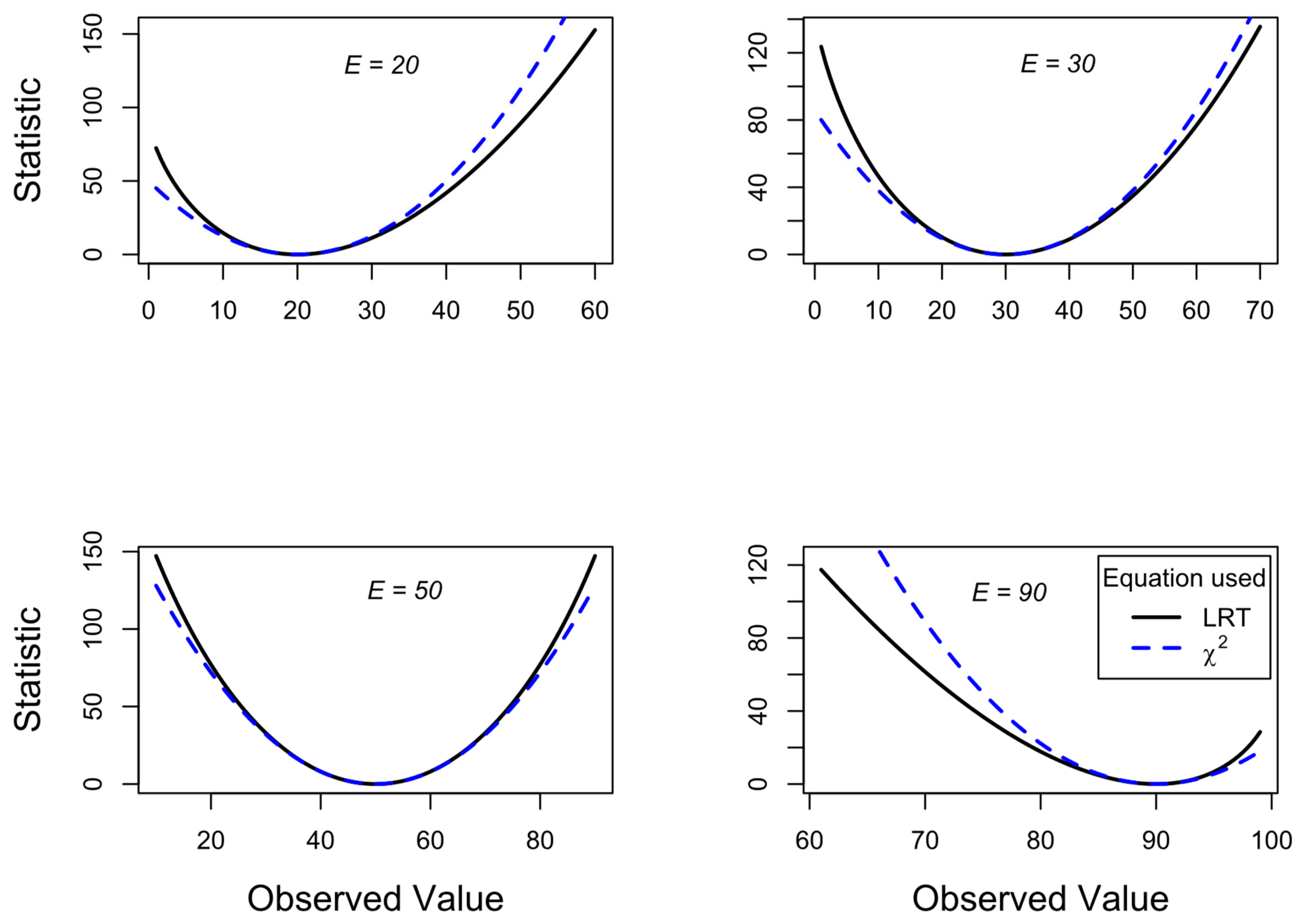
By specifying expected values for the top left cell in the 2 × 2 table (cell a), we can then plot the calculated chi-square for LRT and χ2 test for a range of observed values from 1 to 99. Figure 3 shows this for different expected cell a values of 20, 30, 50 and 90 (see insets showing E). As the expected value approaches their extremes (20 and 90 plots), the LRT statistics for even more extreme observed probabilities become more liberal (higher calculated statistics, giving smaller p values) compared to the χ2 test statistics. In contrast, the LRT statistics become more conservative for observed probabilities that head towards 0.5 and beyond.
Figure 1 and Figure 3 show that as large differences between observed and expected values occur, the lines for LRT and X2 diverge. This is because they are measuring different things. The former is measuring the fit of the proportions while the latter is measuring the variance in the model. Which of these are we typically interested in when doing a 2 × 2 table analysis? Typically, we are interested in whether the proportions match the expected proportions (the null may be determined from the marginal totals). We are much less interested in whether the data are too close to expected frequencies (Stuart 1954). Therefore, we should normally be using the LRT rather than the χ2 test.
Should we be interested in whether the observed frequencies too closely match frequencies specified by a particular hypothesis, then we should use the χ2 test. This scenario is much less frequent.
3. Empirical Data
Let us consider a particular set of data. Imagine that a large study was done on 20 thousand patients, half received a treatment and half received placebo. From this study we obtained a contingency table:
| Death | Survival | ||
| Treatment | 80 | 9920 | 10000 |
| Placebo | 120 | 9880 | 10000 |
| 200 | 19800 | 20000 |
Despite the rather modest odds ratio of 0.66 indicating a protective effect of the treatment, the result was highly statistically significant because of the large sample size with X2(1) = 8.08, p = .004 (using LRT we get a similar result X2(1) = 8.13, p = .004).
Now, a small modification was made to the treatment, and some thought it might not make a difference. A smaller replication study was done with a tenth of the number patients, giving the following data
| Death | Survival | ||
| Modified treatment | 3 | 997 | 1000 |
| Placebo | 10 | 990 | 1000 |
| 13 | 1987 | 2000 |
The general effect was the similar but achieved a better odds ratio of 0.30. The usual analysis of these data would give a non-statistically significant result with the χ2 test:
X2(1) = 3.79, p = .051
But would be statistically significant with the LRT:
X2(1) = 4.00, p = .045
Since we are interested in proportions here, we should use the LRT result.
Although we could claim that there was a statistically significant beneficial effect of the modified treatment in the smaller sample, we don’t know if the result differs from the previous large-scale study that used the original form of the treatment. To do this we need to first obtain probabilities for each outcome based upon the original study
| Death | Survival | |
| Treatment | 0.004 | 0.496 |
| Placebo | 0.006 | 0.494 |
The expected frequencies generated from these probabilities using the smaller sample, N = 2000, can then be used to calculate our two test statistics.
The χ2 test is non-statistically significant:
X2(1) = 3.49, p = .062
Again, the LRT is statistically significant, this time by a larger margin:
X2(1) = 4.50, p = .034
Since we are interested in proportions (not variances) then we should use the statistically significant LRT result which suggests that the modified treatment is even better than the original treatment. This result is predicted from Figure 3 (top left panel) where there was a low expected value of 8 and an even lower observed value of 3 (resulting in more statistical power for the LRT versus the χ2 test).
4. Discussion
Both theoretical and empirical grounds, as demonstrated above, indicate that the correct test to test independence in a 2 × 2 contingency table is the LRT. In this test we are interested the two binomial proportions (typically they are equal for the null hypothesis).
Sokal & Rohlf in their seminal textbook (Sokal and Rohlf 1969) wrote about the advantages of the LRT (which they call the G test) in their 1st edition p550:
“…as is explained at various places throughout the text, G has general theoretical advantages over X2, as well as being computationally simpler for tests of independence. It may be confusing to the reader to have two alternative tests presented for most types of problems and our inclination would be to drop the chi-square tests entirely and teach G only. …to the newcomer to statistics, however, we would recommend that he familiarize himself principally with the G-tests.”
After this proselytizing, their 3rd edition of 1995 (Sokal and Rohlf 1995) p686 merely states:
“…as we will explain, G has theoretical advantages over X2 in addition to being computationally simpler, not only by computer but also on most calculators.”
The calculational advantages are minimal now that most statistical packages routinely calculate both statistics. It is easily (and correctly) argued that the differences seen here between the two tests are marginal and might make little difference. The counterargument is to say that researchers feel more comfortable using a theoretically justified technique that is statistically testing what they are out to test. As Edwards (P 193) comments bitingly: “The original test [χ2] gave the ‘right’ answer, but for the wrong reason. This is, of course, an expected characteristic of a procedure which has stood the test of time; it is only when we examine the problem closely that we realise the difficulties.” (Edwards 1992).
A second argument is that, as the χ2 test is so frequently used (abused), marginal significant or non-significant effects will be incorrectly reported one way or the other in a proportion of these tests. Decisions over whether effects are present often depend on the 5% significance level, and as such will influence whether a paper is published, a medical treatment adopted, or a research grant awarded.
The χ2 test should be reserved for testing if the variance in the model is too low, as in determining whether the observed values match too closely the expected values. This is not routinely of interest. It can, for example, be important is assessing data integrity (Edwards 1986b; MacDougall 2014; Seaman and Allen 2018).
A more consistent and coherent approach would be to calculate the log likelihood ratio (S) from the categorical data according to expected values suggested by the model. The evidential approach was endorsed by Fisher later in his life when he wrote (Fisher 1956):
“…it is important that the likelihood always exists, and is directly calculable. It is usually convenient to tabulate its logarithm…”
Directly calculable because there is no need to calculate the tail probability integral.
The evidential approach was strongly promoted by Edwards in 1972 (Edwards 1972) and an expanded edition published in 1992 (Edwards 1992). Additional arguments and perspectives were supplied by Royall (Royall 1997). More recently the approach has been strengthened by further elaboration in books and articles (Taper and Lele 2004; Taper and Ponciano 2016; Dennis et al. 2019; Markatou and Sofikitou 2019; Cahusac 2020; Taper et al. 2021; Taper, Ponciano, and Toquenaga 2022) . Hypothesis tests focusing on one hypothesis to be rejected (e.g. significance testing) but cannot actually be supported. Such tests have a constant probability of a Type 1 error if the hypothesis is true, irrespective of sample size. This contrasts with the evidential approach where the relative support of hypotheses can be determined, and the probabilities of weak and misleading evidence for one hypothesis versus another, decreases as sample size increases (Royall 2000; Dennis et al. 2019).
In the context of the present paper, the evidential approach would calculate S values using Equations (2) and (6) to test proportions and variance respectively. In most research only the first of these would be required. The second equation would be used to assess whether the fit of the data to the model is closer than expected (implemented in statistical platform jamovi (version 2.4) (retrieved from https://www.jamovi.org accessed 21 November 2023) in the module named jeva (https://blog.jamovi.org/2023/02/22/jeva.html accessed 21 November 2023)). In this framework the support values obtained would be assessed by reference to the table below giving relative strengths of evidence (Goodman 1989; Cahusac 2020).
| S | Interpretation H1 vs H2 |
| 0 | No evidence either way |
| 1 | Weak evidence |
| 2 | Moderate evidence |
| 3 | Strong evidence |
| 4 | Extremely strong evidence |
Consent Statement/Ethical Approval
Not required.
Declaration of Competing Interest
I have no conflict of interest or competing interest to declare.
Submission Declaration
This work is entirely my own and has not been submitted elsewhere.
Supplementary Materials
The following supporting information can be downloaded at the website of this paper posted on Preprints.org.
Funding
No funding was received for this work.
References
- Agresti, A. (2013), Categorical data analysis (3rd ed.): John Wiley & Sons.
- Armitage, P., Berry, G., and Matthews, J. N. S. (2002), Statistical Methods in Medical Research (Vol. 4): WileyBlackwell.
- Cahusac, P.M.B. (2020), Evidence-Based Statistics: An Introduction to the Evidential Approach – from Likelihood Principle to Statistical Practice, New Jersey: John Wiley & Sons.
- Cochran, W.G. (1936), "The X2 Distribution for the Binomial and Poisson Series with Small Expectations," Annals of Eugenics, 7 (3), 207-217. [CrossRef]
- Dennis, B., Ponciano, J. M., Taper, M. L., and Lele, S. R. (2019), "Errors in Statistical Inference Under Model Misspecification: Evidence, Hypothesis Testing, and AIC," Frontiers in Ecology and Evolution, 7. [CrossRef]
- Edwards, A. (1986a), "More on the too-good-to-be-true paradox and Gregor Mendel," Journal of Heredity, 77 (2), 138-138.
- Edwards, A.W.F. (1972), Likelihood, Cambridge: Cambridge University Press.
- --- (1986b), "Are Mendel's Results Really Too Close?," Biological Reviews, 61 (4), 295-312. [CrossRef]
- --- (1992), Likelihood: expanded edition (Vol. 2nd edition), Baltimore: John Hopkins University Press.
- Fisher, R.A. (1922), "On the mathematical foundations of theoretical statistics," Philosophical Transactions of the Royal Society of London. Series A, Containing Papers of a Mathematical or Physical Character, 222 (594-604), 309-368.
- Fisher, R.A. (1936), "Has Mendel's work been rediscovered?," Annals of Science, 1 (2), 115-137. [CrossRef]
- Fisher, R.A. (1950), "The significance of deviations from expectation in a Poisson series," Biometrics, 6 (1), 17-24.
- Fisher, R.A. (1956), Statistical Methods and Scientific Inference (1st ed.), Edinburgh: Oliver & Boyd.
- Goodman, S.N. (1989), "Meta-analysis and evidence," Controlled Clinical Trials, 10 (2), 188-204.
- Goodman, S. N., and Royall, R. M. (1988), "Evidence and Scientific Research," American Journal of Public Health, 78 (12), 1568-1574. [CrossRef]
- Jeffreys, H. 1936. Further significance tests. In Mathematical Proceedings of the Cambridge Philosophical Society: Cambridge University Press.
- MacDougall, M. (2014), "Assessing the Integrity of Clinical Data: When is Statistical Evidence Too Good to be True?," Topoi, 33 (2), 323-337.
- Markatou, M., and Sofikitou, E. M. (2019), "Statistical distances and the construction of evidence functions for model adequacy," Frontiers in Ecology and Evolution, 7, 447.
- Neyman, J., and Pearson, E. S. (1928), "On the use and interpretation of certain test criteria for purposes of statistical inference," Biometrika, 175-240, 263-294.
- Neyman, J., Pearson, E. S., and Pearson, K. (1933), "On the problem of the most efficient tests of statistical hypotheses," Philosophical Transactions of the Royal Society of London. Series A, Containing Papers of a Mathematical or Physical Character, 231 (694-706), 289-337. [CrossRef]
- Pearson, K. (1900), "On the criterion that a given system of deviations from the probable in the case of a correlated system of variables is such that it can be reasonably supposed to have arisen from random sampling," The London, Edinburgh, and Dublin Philosophical Magazine and Journal of Science, 50 (302), 157-175. [CrossRef]
- Royall, R. (2000), "On the Probability of Observing Misleading Statistical Evidence," Journal of the American Statistical Association, 95 (451), 760-768. [CrossRef]
- Royall, R.M. (1997), Statistical Evidence: a Likelihood Paradigm, London: Chapman & Hall.
- Seaman, J. E., and Allen, I. E. (2018), "How Good Are My Data?," Quality Progress, 51 (7), 49-52.
- Sokal, R. R., and Rohlf, F. J. (1969), Biometry: The principles and practice of statistics in biological research, San Francisco: W. H. Freeman and Company.
- --- (1995), Biometry: the principles and practice of statistics in biological research (3rd ed.), New York: W. H. Freeman and Company.
- --- (2009), Introduction to Biostatistics (2nd ed.), New York: Dover Publications, Inc.
- Stuart, A. (1954), "Too Good to be True?," Journal of the Royal Statistical Society: Series C (Applied Statistics), 3 (1), 29-32. [CrossRef]
- Taper, M. L., and Lele, S. R. (eds). (2004), The Nature of Scientific Evidence: Statistical, Philosophical, and Empirical Considerations: University of Chicago Press.
- Taper, M. L., Lele, S. R., Ponciano, J. M., Dennis, B., and Jerde, C. L. (2021), "Assessing the global and local uncertainty of scientific evidence in the presence of model misspecification," Frontiers in Ecology and Evolution, 9, 679155.
- Taper, M. L., and Ponciano, J. M. (2016), "Evidential statistics as a statistical modern synthesis to support 21st century science," Population Ecology, 58 (1), 9-29.
- Taper, M. L., Ponciano, J. M., and Toquenaga, Y. 2022. Evidential Statistics, Model Identification, and Science. Frontiers Media SA.
- Wilks, S.S. (1938), "The Large-Sample Distribution of the Likelihood Ratio for Testing Composite Hypotheses," The Annals of Mathematical Statistics, 9 (1), 60-62.
- Williams, D.A. (1976), "Improved likelihood ratio tests for complete contingency tables," Biometrika, 63 (1), 33-37. [CrossRef]
- Woolf, B. (1957), "The log likelihood ratio test (the G test)," Annals of Human Genetics, 21 (4), 397-409. [CrossRef]
Figure 1.
Calculated statistics plotted for 2 × 2 contingency table with N = 200 and all marginal totals fixed at 100. The observed values for one of the cells is varied from 1 to 99, while expected values are 50 for all cells. The plots for the LRT statistic (Equation (3)) is shown by the black continuous line, X2 test (Equation (1)) is shown by the blue dashed line, and the 2 x Svar (Equation (6)) is shown by the red dotted line. Applying Williams’s correction (Williams 1976) to the LRT has negligible effect, and produces a line that closely overlaps the LRT line.
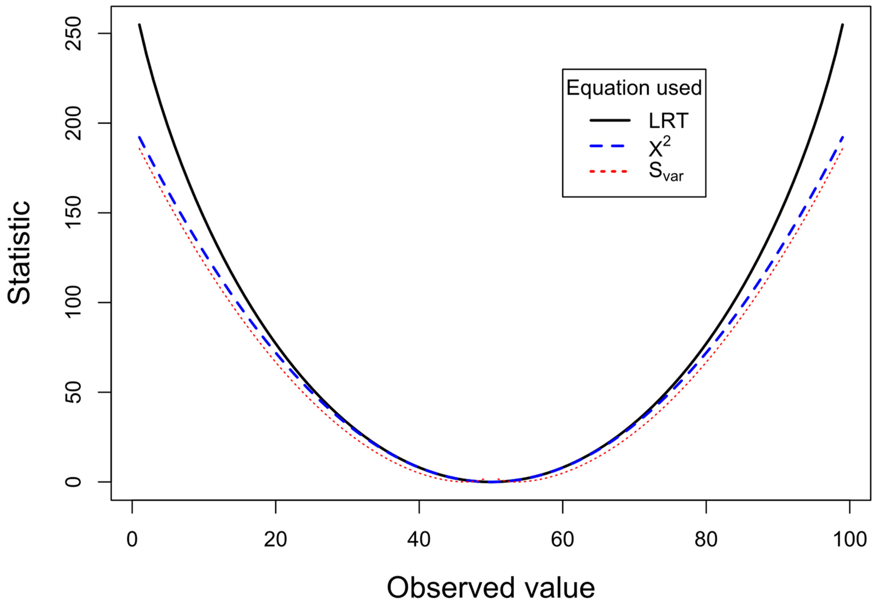
Figure 2.
The same plots as in Figure 1 but on an expanded horizontal scale from 40 to 60. The LRT and X2 test curves overlap very closely, reaching 0 when observed and expected values equalize at 50. In contrast, the 2 x Svar line increases dramatically as these probabilities equalize (and is ∞ when equal).
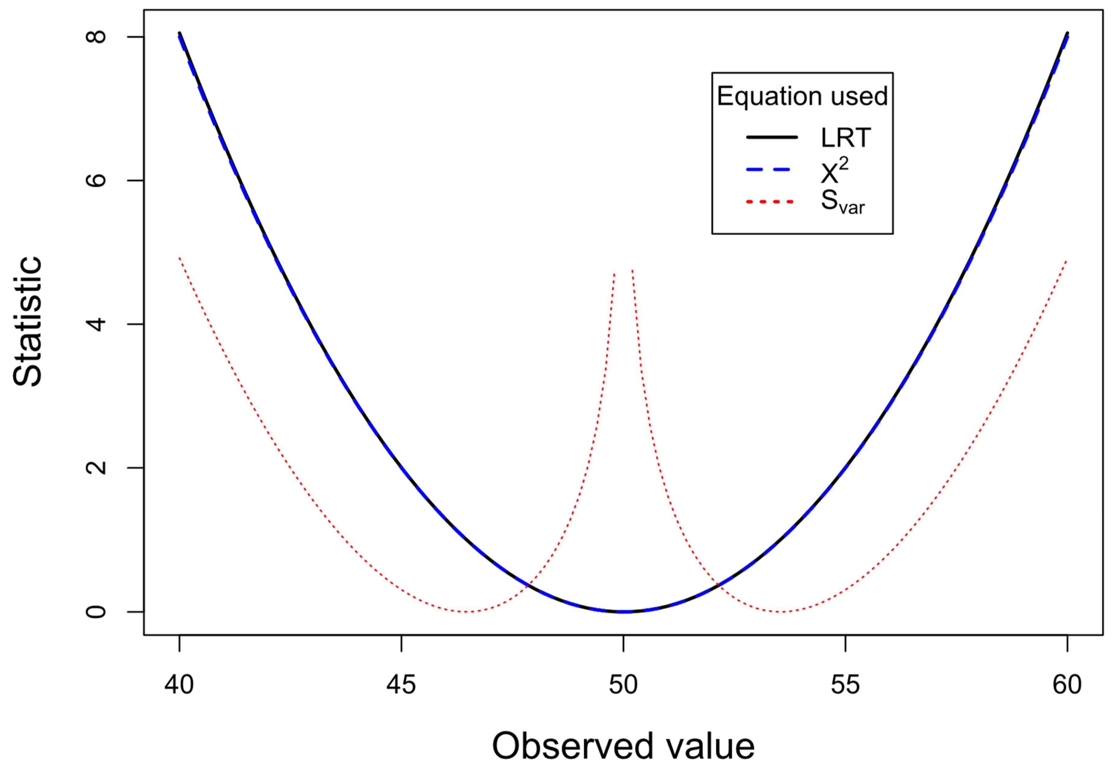
Figure 3.
The statistic using LRT (Equation (3), black continuous line) and X2 test (Equation (1), blue dashed line) are plotted for different fixed expected values (see inset expected (E) values from 20 to 90), where the observed values vary in each plot. Plots use 2 × 2 contingency table data where N = 200 and all marginal totals fixed at 100. The plot for E = 50 is similar to that shown in Figure 1, but without the 2 x Svar line. For display purposes different scales are used for vertical and horizontal axes in each plot. R code for this and other figures is available in Supplementary data.
Disclaimer/Publisher’s Note: The statements, opinions and data contained in all publications are solely those of the individual author(s) and contributor(s) and not of MDPI and/or the editor(s). MDPI and/or the editor(s) disclaim responsibility for any injury to people or property resulting from any ideas, methods, instructions or products referred to in the content. |
© 2023 by the authors. Licensee MDPI, Basel, Switzerland. This article is an open access article distributed under the terms and conditions of the Creative Commons Attribution (CC BY) license (http://creativecommons.org/licenses/by/4.0/).
Copyright: This open access article is published under a Creative Commons CC BY 4.0 license, which permit the free download, distribution, and reuse, provided that the author and preprint are cited in any reuse.


