Submitted:
19 November 2023
Posted:
22 November 2023
Read the latest preprint version here
Abstract
The experiment proposed by Bose et al aims to show the non classicality of gravity through entanglement. This paper seeks to establish optimal conditions under which the entanglement would be maximized. The assumptions made by Bose et al to come to the conclusion of quantized gravity would also be discussed along with alternate conclusions that could arise from the experiment.
Keywords:
quantum gravity
; gravitational entanglement
; semiclassical gravity
1. Introduction
In the realm of theoretical physics, quantum mechanics and quantum field theory have been able to describe three out of four fundamental known forces till now which are the electromagnetic interaction, the strong force, and the weak force. Gravity, however, still does not have a complete theoretical model. Our current model of gravity is based on Einstein’s General Theory of Relativity which has been remarkably accurate in describing many phenomena from the bending of light around mass to gravitational waves. However a fundamental problem we face is that space-time interacts with energy-momentum which are properties of fundamental particles which are currently best described by the quantum theory. General Relativity and Quantum Theory are incompatible models due to a variety of reasons [1], thus we must look for a way to introduce gravity to quantum physics.
In this paper we would look at an experimental proposal that aims to show that gravity can influence matter at quantum scales through the double Stern Gerlach Interferometer experiment devised by Bose et al in their paper [2]. This experiment might be able to show how gravitational field could cause entanglement between two particles. The first portion would look at the experimental parameters that would maximize spin entanglement in the experiment suggested by Bose et al under optimal conditions. Later we discuss what the implications of this experiment are and exploring further possible models.
2. Double Stern Gerlach Spin Entanglement
As suggested in Ref. [2], we keep two test masses in superposition of spacially localized states and . Their evolution happens under gravitational interaction and all other forces are minimized. These two states are localized Gaussian wavepackets and due to their relatively small diameters with respect to their distances and , we can assume .
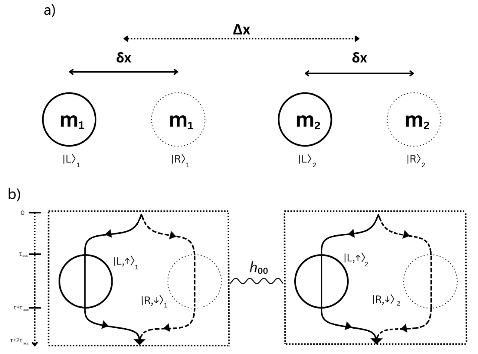
In this setup, we take two masses and with the centers of the left and right states of both the particles separated by the distance as shown in the figure.
Closest distance between and is and farthest distance between and is .
The Classical gravitational potential energy is .
The initial state at is:
Figure 1.
Schematic depiction of the double Stern-Gerlach experiment as proposed by Bose et al. (a) Two mesoscopic particles of equal mass in this case in superposition of two spatially localized states . (b) Evolution of states in SG interferometer into spin entangled states Only the component of energy-momentum tensor is non-negligible due to speeds much slower than the speed of light c[2], hence only component evolves (where is the small perturbation in linearized gravity , being the Minkowskian metric.)
Using the Schrödinger’s equation :
The general solution is found to be when the Hamiltonian is time-independent and is the unitary time-evolution operator.
As E is an eigenvalue of the Hamiltonian, we can write the final state as At , the state evolves to:
Where
and .
A state is said to be entangled if it cannot be factorized (non-separable) to be written as a product of states such as (a separable state).
If we try to factorize Eq(3), we obtain:
The condition for this to be completely factorizable would be if means where n is an arbitrary integer.
Therefore for the state to be entangled,
This gives us the entanglement condition:
The SG interferometer accelerates the particles through a magnetic gradient for a time and then the magnetic field is switched off for a greater amount of time enough to entangle both the superposition states.
In this process, the two joint states of the test masses evolve as shown in Eq.(1) and Eq.(3) the orbital states and get replaced by the spin-orbital qubit states and .(Ref.[2]).
Replacing the states in Eq.(3) with the spin-orbital states gives us:
In the final step, the superposition is brought back through unitary transformations :
This entanglement can be measured using an entanglement witness which is discussed later in Appendix A. If satisfies a certain condition for example exceeding unity in the one Bose et al. suggested, then the state is proven to be entangled.
3. Minimization of Casimir-Polder Interaction
While performing the experiment, it is important to reduce extra noise that may present itself due to other forces between the two particles we are using. One of them is the Casimir force which we will try to reduce.
We will be taking a linear setup for the experiment[3] and the particles as diamond nanoparticles of mass .
The formula for the Casimir force between two neutral dielectric particles is
Where R is the radius of the particles, is the minimum distance between them, c is the speed of light in vacuum (m/s), ℏ is reduced Planck’s constant (Js)and is the dielectric constant (∼ 5.7 for diamonds).
Thus we need the minimum distance between the entangled particles to be for the Casimir force to be negligible (one order of magnitude lower than gravitational force in this case).
4. Conditions for Maximal Entanglement
We will be converting the quantum state to a density operator () in order to perform certain operations on it.
The state can be written as
Here and
The density matrix is evaluated to be
The bipartite von Neumann entropy can help us find the maximally entangled state of a quantum system and is represented by
Where and are the reduced density matrices.
The reduced density matrix was calculated to be:
The system is maximally entangled when and are maximally mixed[4] which is achieved when they are diagonal matrices with diagonal elements as where d is the dimension of the Hilbert space of the basis (which is 2 in our case).
To get these conditions, we set the non-diagonal entries to 0 first:
and
This gives us two equations
They can be written as
By collecting the real and imaginary parts of the expressions.
For to be 0, and (where Re and Im are the real an imaginary components of the complex number respectively)
Looking at the imaginary part,
This implies that Which means either
or
where k is an arbitrary integer.
Substituting Eq(10) in the real part,
This is not a satisfactory condition as for only some values of
Thus we can assume, This leads us to using Eq(11) as follows:
And that satisfies the given conditions, therefore
This is our condition for non-diagonal elements being 0. Now to verify for maximally mixed state, we can substitute these values in the reduced density matrix.
So
By analogy with the classical entropy formula, the entanglement entropy has the following bounds:
As the system saturates the upper pound, the state is maximally entangled.
Figure 2.
Plot of Entanglement Entropy as a function of (from 0 to ) and (from to ). It can be seen that the entropy achieves its maximum value of when the sum of the phases approach .
Figure 2.
Plot of Entanglement Entropy as a function of (from 0 to ) and (from to ). It can be seen that the entropy achieves its maximum value of when the sum of the phases approach .
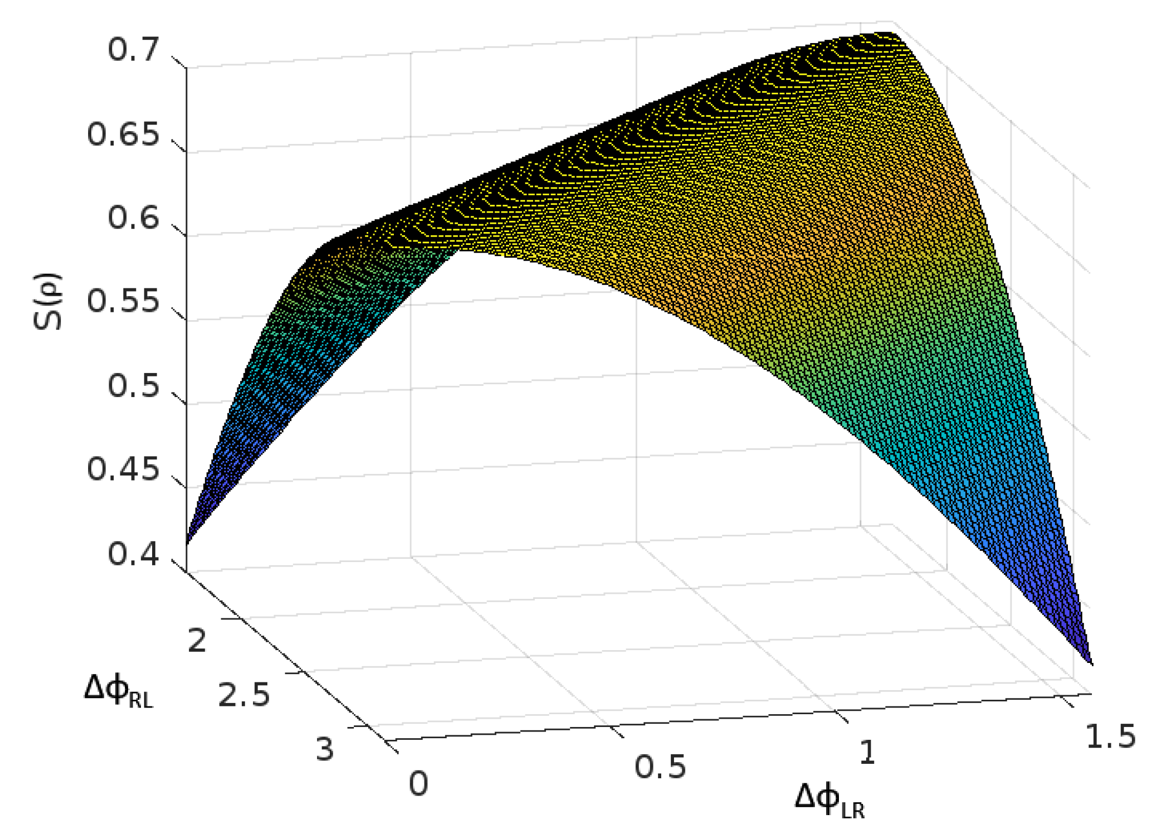
Now we can substitute the values of the phases to get an expression for the distances. For simplicity, we will take in Eq(12).
gives
And finally,
The expression for the distance between the left and right states is[2]:
Where is the electronic g-factor, is the Bohr magneton, is the magnetic field gradient in the x-direction. The mass of the particles we are taking is kg, the magnetic field gradient is , is the time the masses are subjected to the magnetic field gradient and is a variable.
Substituting the distance for minimized CP-effect, , we get:
As the experiment cannot be completely free from outside interaction, there would always be some sort of decoherence in the system. The collisional decoherence time is approximately of the same magnitude as the total fall time of the particle [2]. This will lead to a strong loss of coherence which will interfere with the gravitational entanglement. To minimize this, we can minimize the total time taken for the particle to fall (
Minimizing by a simple python program mentioned in Appendix C gives and Using these values, we can obtain the distances between the entangled states as
Calculating the phase values:
This gives
These values can be substituted in Eq(12) to verify that the maximal entanglement conditions are met:
Some rounding error of % persists but it is almost negligible.
5. Discussion
In order to make inferences from the proposed experiment, we will first need to know its assumptions and limitations.
The main theoretical assumptions of the Bose et al [2] paper is that the gravitational interaction between two masses is mediated by a gravitational field (not a direct action at a distance) and that entanglement between two systems cannot be created by Local Operations and Classical Communication (LOCC).
Another assumption made by them is using the Newtonian potential for mediating the gravitational entanglement which is not the true degree of freedom of the gravitational field and hence might have affected the implications of the experiment. (Discussed thoroughly in Ref. [5])
Based on the given assumptions, the entanglement generated by gravity would be non-classical. However, even if it eliminates the possibility of a completely classical model of gravity, it does not strictly imply that gravity is quantum and a semi-classical model of a gravity is still a valid possibility.
Due to the success of the general theory of relativity in explaining gravity, a good start to uncovering the mystery would be to look at the semi-classical models of gravity. The classical Einstein’s Field Equations are
Where is the Einstein Tensor and is the stress-energy tensor. However in a quantum scenario, the stress-energy tensor has to be an operator which would be inconsistent with the left half of the equation which is why we take its expectation value according to Møller-Rosenfeld [6,7], giving us a scalar value of the operator.
Here . We do run into technical difficulties in this equation one of them being that the expectation value of the energy-momentum tensor is not conserved while the Einstein tensor is (). Thus we need to renormalize which would give us and other conditions discussed by Wald [8].
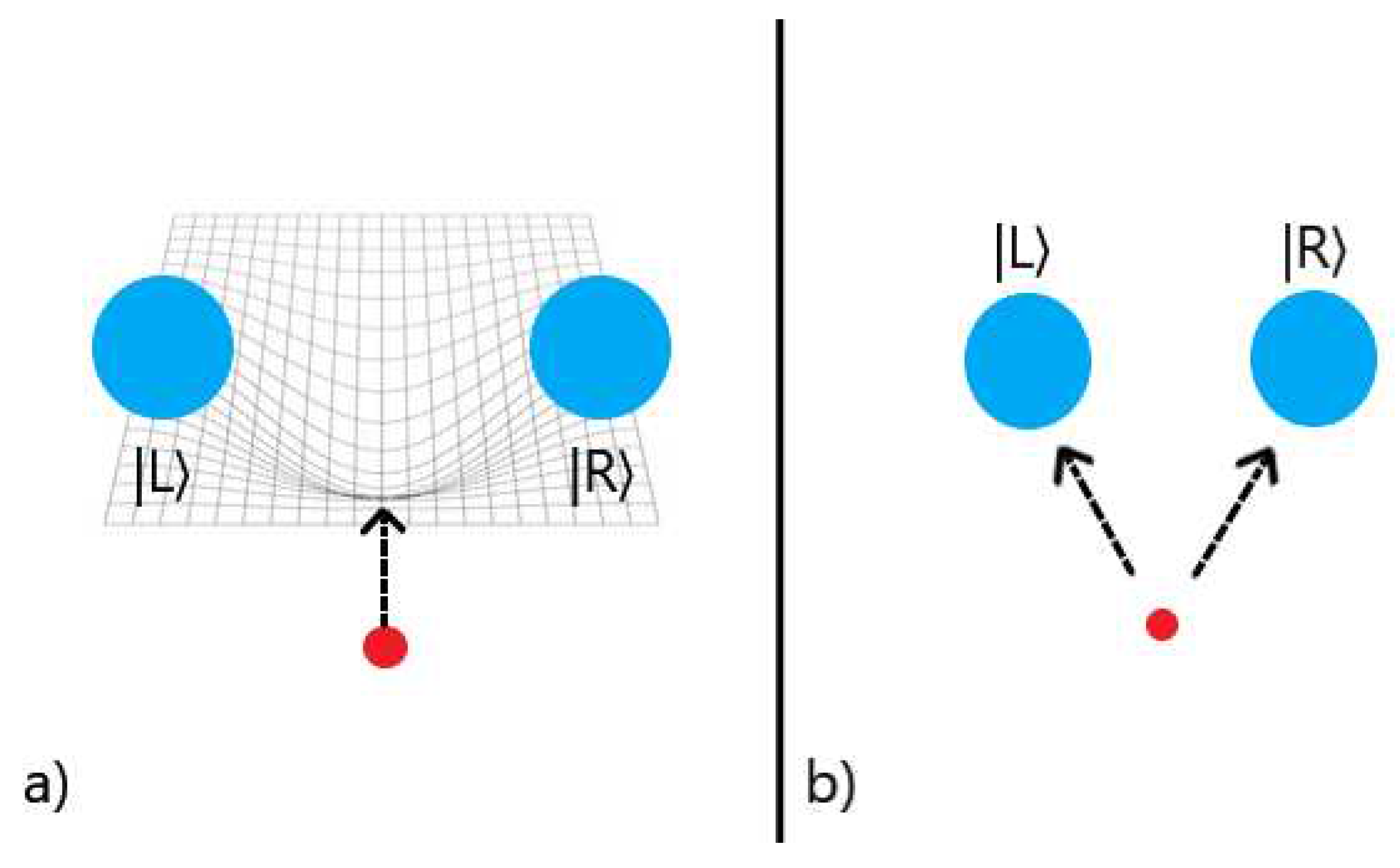
Another flaw with the field equations semi-classical gravity is that the expectation value in some cases implies that the net curvature of the superposition states would be averaged out in the center and we would expect a test particle to move towards that center. This is not what experiments have shown so it is a massive downside of this model. ([9,10]) Due to the limitations of this model, other semi-classical models have also been proposed, an important one being the stochastic model [11].
Figure 3.
a) Expected behaviour in Møller-Rosenfeld semi-classical gravity vs b) Observed behaviour of particle in superposition
Figure 3.
a) Expected behaviour in Møller-Rosenfeld semi-classical gravity vs b) Observed behaviour of particle in superposition
Two of the current leading models for quantum gravity are the Loop Quantum Gravity model [12] and the String Theory [13] which would not be discussed here being beyond the scope of this paper.
In conclusion, new experiments might help us eliminate more erroneous models and get closer to the right one.
Acknowledgments
I would like to express my deepest gratitude to Doctor Damián Pitalúa-García for his invaluable guidance and mentorship, which has been instrumental in helping me build a solid foundation in quantum physics. His expertise and insights into the key concepts explored in this paper have been indispensable in shaping my understanding and contributing to the quality of this work. I am also thankful to Mr. C.K. Campbell for helping me understand certain aspects of the experiment and for assisting me in locating essential research papers that served as crucial background reading for my paper and overall research.
Appendix A: Entanglement Witness
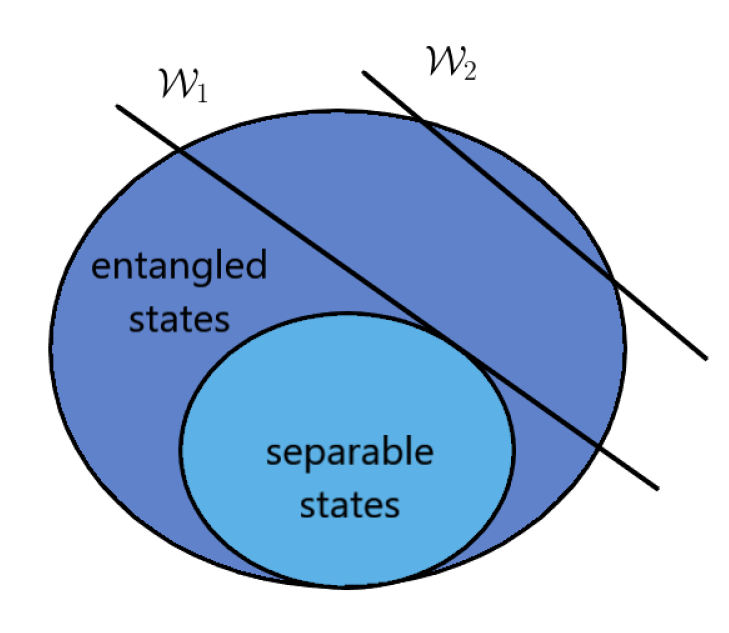
Entanglement witnesses are functions (often applied on the density matrix) to show that a state is entangled. These witnesses are useful as they do not give false positives and are helpful in confirming whether a given state is entangled. Of course a witness might not be able to detect all entangled states but they can be optimized to detect most of them.
Figure 4.
Diagram depicting convex set of quantum states including separable and entangled states. The witness detects more states than and hence, is more efficient.
Figure 4.
Diagram depicting convex set of quantum states including separable and entangled states. The witness detects more states than and hence, is more efficient.
Entanglement Witness suggested by Bose et al [2] is .
Their condition is that if then the state is proven to be entangled. To verify this we will use the bell states as they are maximally entangled.
For :
Similarly,
As we can observe even the maximally entangled bell state does not exceed unity for this entanglement witness hence it might not be useful for the states calculated in this paper which is why the need to use a different witness arises.
Here we can use the common entanglement witness for entangled states.
The state is Evaluating the witness for this state:
As , we can say that the obtained state is definitely entangled.
Appendix B: Density Matrix Calculations
For notational convenience, we will be taking and .
In Section 4, the quantum state used is
The conjugate transpose of this ket is the corresponding bra:
The density operator
This can be converted to matrix notation using the following:
Similarly,
Adding the terms,
The reduced density matrix is defined as
Where is the identity operator in and is the partial trace of the density matrix.
As when , this leaves us with
In matrix form:
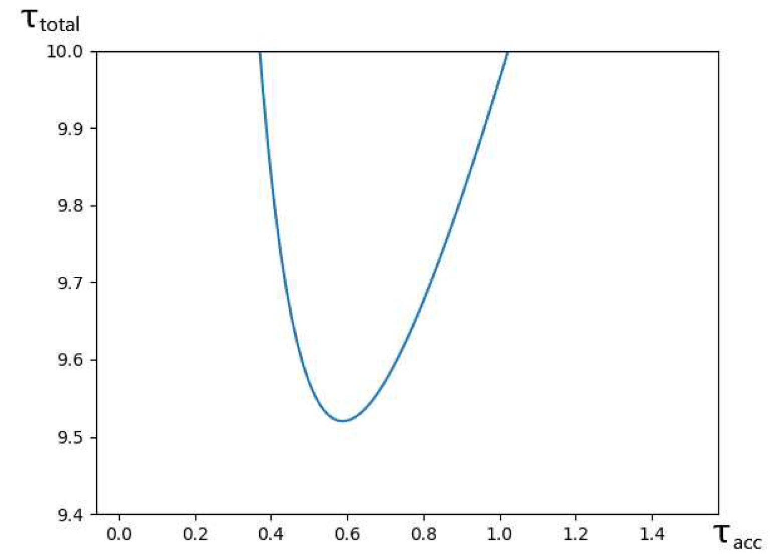
Appendix C: Minimization of Time Taken
Our minimization expression is .
The minimization constraint is Eq(15) which we will be simplifying by assigning variables to the numerical constants
This reduces Eq(15) to:
Now this can be rearranged to define as a function of as
By substituting Eq(18) in our minimization expression, we obtain a function in one variable which can be minimized using a simple python code.
This gives , and .
Figure 5.
Graph of as a function of .
References
- Macías, A. On the incompatibility between general relativity and quantum theory. 2008. Available online: https://pubs.aip.org/aip/acp/article-abstract/977/1/3/662451/On-the-incompatibility-between-General-Relativity?redirectedFrom=fulltext.
- Bose, S.; Mazumdar, A.; Morley, G.W.; Ulbricht, H.; Toro, M.; Paternostro, M.; Geraci, A.A.; Barker, P.; Kim, M.S.; Milburn, G.J. Spin Entanglement Witness for Quantum Gravity. Physical review letters 2017, 119 24, 240401. [Google Scholar] [CrossRef]
- Schut, M.; Grinin, A.; Dana, A.; Bose, S.; Geraci, A.A.; Mazumdar, A. Relaxation of experimental parameters in a Quantum-Gravity Induced Entanglement of Masses Protocol using electromagnetic screening. https://arxiv.org/pdf/2307.07536.pdf. 2023.
- Nielsen, M.A.; Chuang, I.L. Quantum Computation and Quantum Information; Cambridge University Press, 2000; Available online: https://www.cambridge.org/highereducation/books/quantum-computation-and-quantum-information/01E10196D0A682A6AEFFEA52D53BE9AE#overview.
- Charis Anastopoulos and Bei-Lok, Hu. Comment on ”a spin entanglement witness for quantum gravity” and on ”gravitationally induced entanglement between two massive particles is sufficient evidence of quantum effects in gravity”. 2018. [Google Scholar]
- Lichnerowicz, M.A.; Tonnelat, M.A. (Eds.) Proceedings, Les théories relativistes de la gravitation : actes du colloque international (Relativistic Theories of Gravitation): Royaumont, France, June 21-27, 1959; Paris: Paris, 1962. [Google Scholar]
- Rosenfeld, L. On quantization of fields. Nucl. Phys. 1963, 40, 353–356. [Google Scholar] [CrossRef]
- Wald, R.M. Trace anomaly of a conformally invariant quantum field in curved spacetime. Phys. Rev. D 1978, 17, 1477–1484. [Google Scholar] [CrossRef]
- Eppley, K.R.; Hannah, E. The necessity of quantizing the gravitational field. Foundations of Physics 1977, 7, 51–68. [Google Scholar] [CrossRef]
- Page, D.N.; Geilker, C.D. Indirect Evidence for Quantum Gravity. Physical Review Letters 1981, 47, 979–982. [Google Scholar] [CrossRef]
- Martí n, R.; Verdaguer, E. Stochastic semiclassical gravity. Physical Review D 1999, 60. [Google Scholar] [CrossRef]
- Ashtekar, A.; Bianchi, E. A short review of loop quantum gravity. Reports on Progress in Physics 2021, 84, https://iopscience.iop.org/article/10.1088/1361–6633/abed91. [Google Scholar] [CrossRef] [PubMed]
- Seiberg, N.; Witten, E. String theory and noncommutative geometry. Journal of High Energy Physics 1999, 1999, 032–032. [Google Scholar] [CrossRef]
Disclaimer/Publisher’s Note: The statements, opinions and data contained in all publications are solely those of the individual author(s) and contributor(s) and not of MDPI and/or the editor(s). MDPI and/or the editor(s) disclaim responsibility for any injury to people or property resulting from any ideas, methods, instructions or products referred to in the content. |
© 2023 by the authors. Licensee MDPI, Basel, Switzerland. This article is an open access article distributed under the terms and conditions of the Creative Commons Attribution (CC BY) license (http://creativecommons.org/licenses/by/4.0/).
Copyright: This open access article is published under a Creative Commons CC BY 4.0 license, which permit the free download, distribution, and reuse, provided that the author and preprint are cited in any reuse.


