Research on Non-intrusive Load Recognition Algorithm Based on High Frequency Signal Decomposition with Improved VI Trajectory and Background Color Coding

Preprint

Article

Research on Non-intrusive Load Recognition Algorithm Based on High Frequency Signal Decomposition with Improved VI Trajectory and Background Color Coding

Altmetrics

Downloads

Views

Comments

A peer-reviewed article of this preprint also exists.

Rao Fu^*

Rao Fu^*

This version is not peer-reviewed

Submitted:

16 November 2023

Posted:

17 November 2023

You are already at the latest version

Alerts

Abstract

Against the backdrop of the current carbon peaking and carbon neutrality policies, higher requirements have been put forward for the upgrading and construction of smart grids. Non-intrusive load monitoring (NILM) technology is a key technology for advanced measurement systems at the end of the power grid. It obtains detailed power information of the load, without the need for traditional hardware deployment. The key step to solve this problem is load decomposition and identification. This paper first utilized Long Short Term Memory-Denoising Autoencoder(LSTM-DAE) to decompose the mixed current signal on the household busbar and obtain the current signals of multiple independent loads that constituted the mixed current. Then, the obtained independent current signals were combined with voltage signals to generate multi-cycle colored Voltage-Current(VI) trajectories, which were color-coded according to the background. These colored VI trajectories with background colors formed a feature library. When the CNN network was used for load recognition, considering the influence of hyperparameters on recognition results, the BOA algorithm was used for optimization, and the optimized CNN network was employed for VI trajectory recognition. Finally, the proposed method was validated using the PLAID dataset. Experimental results showed that the proposed method exhibited better performance in load decomposition and identification.

Keywords:

Subject: Computer Science and Mathematics - Artificial Intelligence and Machine Learning

1. Introduction

Given the ongoing increase in residents’ electricity consumption, incorporating effective daily electricity usage planning is important to minimize energy waste. In this regard, Non-intrusive load monitoring (NILM) can help identify residents’ electrical appliances and their states, enabling residents to have a better understanding of their electricity consumption behavior and improve their usage patterns [1]. Moreover, NILM can also enhance management and optimization of the demand side of the power grid, aiming to achieve energy saving goals. Therefore, it holds great significance for energy conservation and emission reduction [2]. Unlike traditional methods requiring the installation of multiple sensors, NILM integrates electricity information into a single collection signal, making it more cost-effective and practical [3].

In the past, existing research often treated load decomposition and load identification as two separate monitoring objectives, while overlooking the crucial role of load decomposition in the identification process. Without load decomposition, it was not possible to obtain independent signal sources and compare them effectively with the load feature library. As a result, this study considered load decomposition and load identification as an integrated research subject, where independently obtained current signals from load decomposition served as fundamental data for further research.

In the past, in load identification tasks, Voltage-Current (VI) trajectories were widely used as the most common load features, significantly improving identification accuracy through advanced Convolutional Neural Networks (CNNs). However, traditional VI trajectories had certain limitations. For instance, VI trajectories of different load types exhibited strong similarities. For example, the current waveforms of resistive loads tended to resemble standard sine waveforms, resulting in pronounced similarities in VI trajectories. Additionally, traditional VI trajectories failed to reflect current amplitude information or capture fluctuation issues during load operation.

Therefore, addressing the above-mentioned problems, this paper proposed a method based on LSTM-DAE for decomposing complex mixed signals. Afterwards, by constructing a color encoding VI feature library with a background color, load recognition was performed using a CNN network adjusted by Bayesian Optimization Algorithm (BOA) for hyperparameter tuning. The specific method was as follows:

(1): The high-frequency mixed current signals were decomposed using LSTM-DAE. This paper accurately acquired current signals of each load by exploiting the high sensitivity of LSTM to temporal signal features and the ability of DAE to transform load decomposition problems into denoising problems, which were then utilized as the fundamental data for load recognition.
(2): Colored VI trajectories were generated by plotting VI trajectories obtained from multi-cycle voltage and current data. The R channel represented the normal multi-cycle VI trajectory, the G channel represented the current variation slope between adjacent sampling points, and the B channel represented the rate of power changes. Additionally, the VI trajectory background was color processed based on the difference in current amplitude to obtain a multi-cycle color-encoded VI trajectory feature library with filled background colors.
(3): The VI trajectory feature library was transformed into an n×n image format and input into the AlexNet network for training. Since the traditional AlexNet network was not suitable for load recognition tasks, the BOA algorithm was employed to optimize the network parameters, thus achieving better recognition performance.
(4): The PLAID dataset was utilized in the experiments, and the results demonstrated that the selected six load decomposition accuracies all exceeded 94.

2. Related works

Traditional load decomposition was based on low-frequency data to decompose aggregated data into device-level data without the need for event detection[4]. The Hidden Markov Model (HMM) was a commonly used regression model. Kim et al. validated four HMM extension models and introduced non-electrical characteristics such as load switching duration, load usage frequency, and interdependence among loads, which improved the decomposition accuracy to a certain extent [5]. Kolter et al. applied the Factorial Hidden Markov Model (FHMM) algorithm to establish a load decomposition model, using total current signals as the research object. When a signal change was detected, the signal differences between the load currents were encoded, resulting in the optimal solution for the model and achieving high decomposition accuracy [6]. With the continuous development of deep learning technology, non-intrusive load decomposition models based on deep learning emerged [7]. In 2015, Kelly introduced deep learning methods into the NILM field and coined the term "Neural NILM." Kelly proposed three neural network structures: Long Short-Term Memory (LSTM), Recurrent Neural Network (RNN), and Distributed Agent Environment (DAE), which were effective in handling long time-series data [8]. Roberto improved Kelly’s DAE model by combining it with a median filter, which partially eliminated noise interference and improved the model’s robustness [9]. Odysseas modified Kelly’s LSTM network due to the high number of network neurons, leading to long training times and unsuitability for embedded devices. Instead, the Gated Recurrent Unit (GRU) algorithm was used, reducing the network’s depth while maintaining accuracy and reducing computational complexity [10]. Zhang Chaoyun proposed a load decomposition framework that mapped sequences to individual load points, with aggregated power data of windows as the network’s input and the corresponding single-point load data as the network’s output. This mapping pattern accelerated training speed and improved load decomposition real-time performance [11]. Barsim proposed a general deep decomposition model that automatically adjusted model parameters based on the characteristics of different loads, thus obtaining more accurate load switching state sequences [12]. Piccialli adopted a neural network model with an attention mechanism, which strengthened the correlation between input and output and improved decomposition accuracy [13]. "High-frequency decomposition-1" focused on decomposing high-frequency current signals by transforming the current decomposition problem into blind source separation. It optimally solved the problem using the sparsity of frequency domain signals, which did not rely on prior knowledge but introduced a certain degree of error.

References [14] utilized the Dynamic Time Warping (DTW) algorithm to calculate the similarity between test templates and reference templates, using transient waveforms and power change values of household load switchings as feature quantities for load recognition. Reference [15] clustered load data based on steady-state values and proposed a non-intrusive load recognition method using Feature Weighted K-Nearest Neighbor (FWKNN), which improved feature distance calculations with feature weights and achieved high accuracy. References [16] presented an attention model that combined global and sliding window approaches, employing bidirectional LSTM networks as encoders to extract information, utilizing an attention mechanism to capture the current load information and decode the output decomposition results. Reference [17] encoded different power states of target appliances using a deep recurrent convolutional model, extracting spatiotemporal features of input total load power, and implemented state modeling of different target appliances through transfer learning, achieving significant improvement compared to Markov models. Reference [18] described in detail 8 shape features such as the asymmetry observed in VI trajectories and conducted recognition using hierarchical clustering. Reference [19] used the elliptical Fourier descriptor of VI trajectory contours as input for a classification algorithm. Reference [20], based on [21], introduced a new feature called "span" and compared it with the harmonic content, active power, and reactive power of the current, utilizing four classification algorithms. The results showed that VI trajectories had good recognition capability.

3. LSTM-DAE based load decomposition

3.1. Load decomposition

Load decomposition is the process of decomposing a mixed telecommunications signal into independent telecommunications signals for each load. This paper transformed this process into a denoising problem to obtain accurate information about the current of each load. Assuming there were N loads, the total current at time t was:

I (t) = \sum_{k = 1}^{N} I_{k} (t) + I_{δ} (t)

(1)

where

I (t)

was the total current at the current moment,

I_{k} (t)

was the current generated by the kth load, and

I_{δ} (t)

was the noise disturbance.

Assuming the target load current represented the actual signal and considering the total current signal as the composite of the actual signal and noise interference, the equation could be modified as follows:

I (t) = I_{η} (t) + I_{β} (t)

(2)

where

I_{η} (t)

is the current of the target load and also the real current in the denoising process, and

I_{β} (t)

is the noise in the denoising process, where

I_{β} (t)

is the superposition of the currents of the loads other than the current of the target load and the real noise, expressed as:

I_{β} (t) = \sum_{k = 1}^{N - 1} I_{k} (t) + I_{δ} (t)

(3)

3.2. Denoising Autoencoder

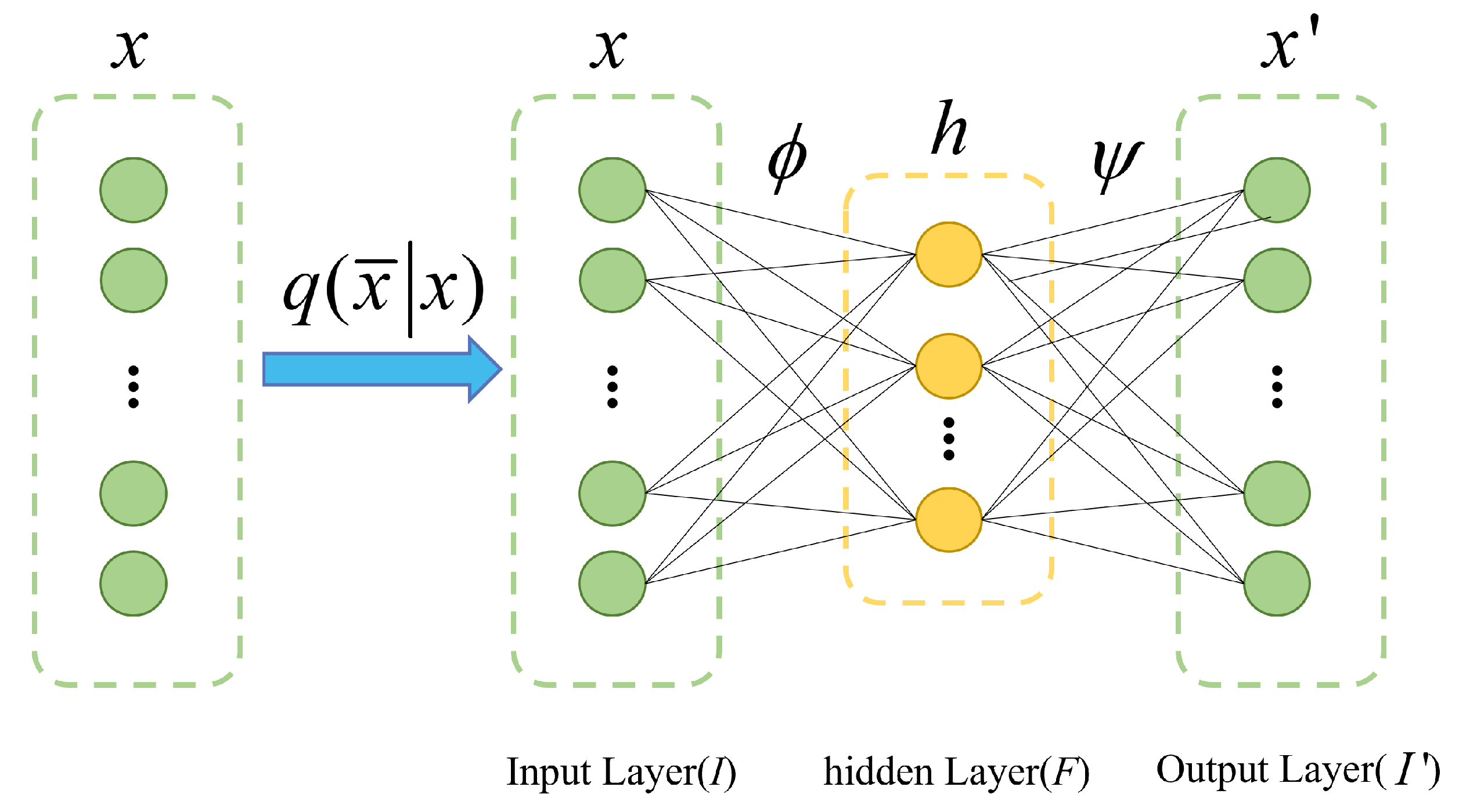
As shown in Figure 1, the Autoencoder (AE) had an equal number of nodes for input and output, aiming to minimize the reconstruction error between the input and output. It consisted of an encoder

ϕ

and a decoder

ψ

, where the encoder mapped the input to a low-dimensional feature space, and the decoder mapped the data from the low-dimensional feature space back to the original input. In Figure 1, x represented the input data to the encoder, h represented the data mapped from x to the hidden feature space, and

x^{'}

represented the data reconstructed by the decoder using the hidden feature space data h. Assuming the input space was

I = R^{n}

(where n was the number of variables), the working principle of an autoencoder could be defined as follows:

\begin{matrix} ϕ : I \to F \\ ψ : F \to I \\ ϕ, ψ = \underset{ϕ, ψ}{argmin} {∥x - x^{'}∥}^{2} \end{matrix}

(4)

where

∥ \cdot ∥

denoted the Frobenius paradigm. Taking the AE with one hidden layer as an example, the encoder mapped the input

x \in I

to the hidden feature space

h \in F = R^{p}

, p was the dimension of the hidden layer), and the mapping process:

h = σ (W x + b)

(5)

where

σ

was the activation function in the encoder,

W

was the weight matrix, and

b

was the bias vector. After the encoder mapped the input variable to the hidden layer, the decoder reconstructed the variable

x^{'}

into a variable of the same size as the input variable x based on the information in the hidden layer h. The mapping process was as follows:

x^{'} = σ^{'} (W^{'} x + b^{'})

(6)

where

σ^{'}

represented the activation function in the decoder, and

W^{'}

and

b^{'}

corresponded to the weight matrix and deviation vector in the decoder. The goal of the self-encoder was to find the process that minimized the residuals between the input and the reconstructed quantity

x^{'}

\begin{matrix} L (x, x^{'}) & = \frac{1}{m} {∥x - x^{'}∥}^{2} \\ = \frac{1}{m} {∥x - σ^{'} (W^{'} σ (W x + b)) + b^{'}∥}^{2} \end{matrix}

(7)

where m represented the number of sample points into the AE network. The optimization problem of the self-encoder could be solved by backpropagation.

Denoising Autoencoder (DAE) was a variant of AE, which was first proposed by Vincent et al [22], and its network structure was shown in Figure 2. The difference with AE was that it used partially corrupted data to train the DAE network in order to recover the real inputs, and its function was to separate the noise in the data to get the real data after removing the noise. The workflow of DAE was as follows:

(1): Obtaining corrupted data by adding noise to normal data or randomly discarding parts of normal data was obtained.

$\tilde{x} = q (\tilde{x} ∣ x)$

(8)
(2): Mapping the corrupted data to the low-dimensional hidden feature space by the self-encoder coding process $h = σ (W x + b)$ .
(3): The decoder decoded the corrupted data’s mapping in the hidden feature space using Equation 6 and obtained the reconstructed data.
(4): The minimization problem of Equation 7 was solved using the backpropagation algorithm.

In this paper, signal decomposition was converted into a denoising problem. Specifically, the mixed current signals were treated as noisy signals, and the independent load signals were seen as real data after undergoing denoising processing.

3.3. Decomposition model based on LSTM-DAE

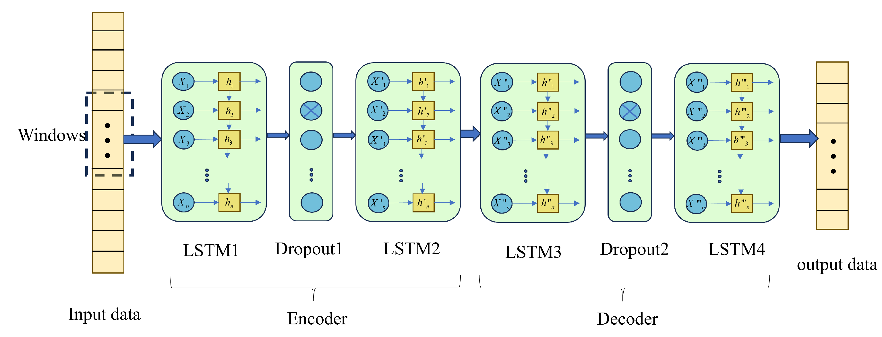
The LSTM network exhibited good performance in extracting features from time series signals. Therefore, LSTM was combined with DAE. The encoder and decoder parts of DAE were respectively composed of dual-layer LSTM and Dropout layers. The input data was the mixed current data, and a sliding window approach was employed, where multiple cycles of mixed current were used as input. This paper selected a window size of 10 cycles to achieve the functionality of seq2seq and obtain the output of independent current. The structure was shown in Figure 3.

4. Load recognition of VI traces based on background color coding

4.1. Construction of VI trajectory pixelization

The VI trajectory referred to the voltage-current relationship curve used to describe the performance characteristics of electrical equipment. Traditional VI trajectory analysis methods mapped the curve onto a unit grid, where each grid cell represented the presence or absence of VI trajectory information (0 or 1). The grid was then transformed into an image, thereby converting the load recognition problem into an image recognition problem for automated identification. However, previous methods only utilized binary values to represent each grid cell, resulting in relatively limited information content. Therefore, this paper proposed an improved approach aimed at enhancing the expressive power of VI trajectory data.

(1): Conventional VI traces typically analyzed changes in a single cycle, which failed to capture the characteristic changes of the load across different operating cycles. Therefore, the paper proposed to utilize 20 consecutive cycles of current-voltage signals to generate VI traces, aiming to provide a more comprehensive reflection of the changes across different cycles.
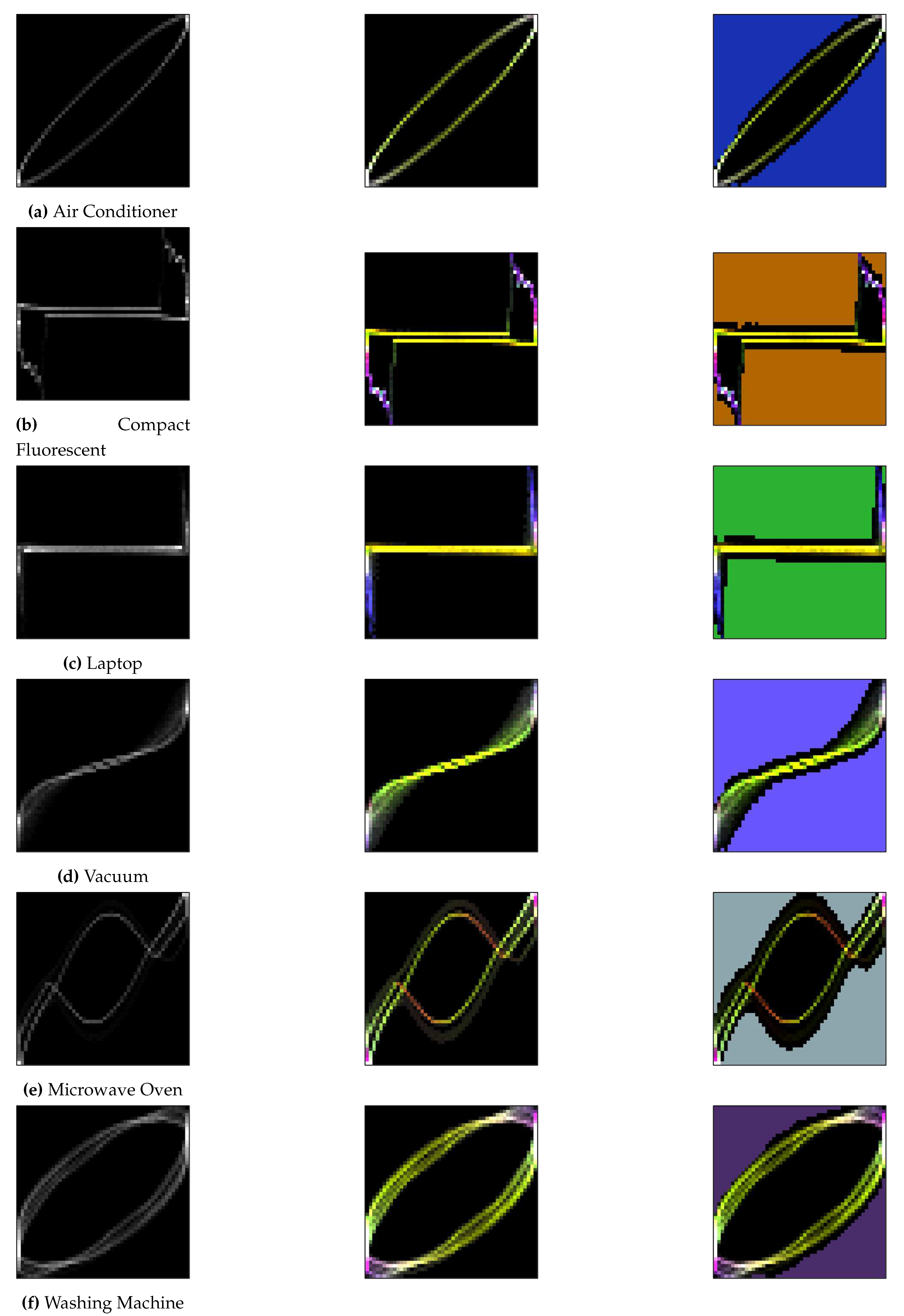
(2): Color coding the VI trajectory: the multi-cycle VI trajectory was represented in red (R channel), the slope of the straight line segment between adjacent sampling points of the VI trajectory was represented in green (G channel), and the instantaneous power value was represented in blue (B channel), thereby generating a VI trajectory image with colored tracks.
(3): Due to the significant differences in current amplitude between certain loads while having similar VI trajectories, and considering that current amplitude is an important load characteristic, this paper proposed assigning different colors to the background of VI trajectories based on the varying current amplitudes in order to highlight the differences in current amplitude.

The specific steps are as follows:

(1): Standardized the voltage and current values, and used the standardized voltage and current data to plot the standardized VI trajectory. The standardization formula was as follows:

$Δ V_{m} = \frac{V_{m}}{max | V |}$

(9)

$Δ I_{m} = \frac{I_{m}}{max | I |}$

(10)

where $| V |$ was the maximum value of voltage in the steady state sequence and max $| I |$ was the maximum value of current in the steady state sequence. $V_{m}$ , $I_{m}$ were the voltage and current values of the mth sampling point in the sequence, and $Δ V_{m}$ , $Δ I_{m}$ were the voltage and current values of the mth sampling point after normalization.
(2): Created the VI trajectory using normalized data, and used the created VI trajectory as the R channel of the colored VI trajectory.
(3): Created the G channel by mapping the slope of the straight line segments to the (0,1) range using the $a r c t a n$ function.

$K_{j} = \frac{i_{f} (j + 1) - i_{f} (j)}{V (j + 1) - V (j)} \times \frac{max (| V |)}{max (|I_{f}|)}$

(11)

$G_{j} = \frac{1}{2} + \frac{arctan (K_{j})}{π}$

(12)

where $K_{j}$ was the slope of the jth straight line segment and $G_{j}$ was the G-channel depth value of the jth straight line segment. The $G_{j}$ was mapped to the VI trajectory to obtain the corresponding G-channel depth value $G_{m, n}$ for each grid, which was then normalized to obtain the G-channel value for each grid point.

${G_{m, n}}^{'} = \frac{G_{m, n}}{max G}$

(13)

$m a x G = max \{G_{1, 1}, G_{1, 2}, G_{1, 3}, \dots, G_{n, n}\}$

(14)
(4): The B channel was created with the following instantaneous power values:

$P_{j} = I_{j} • V_{j}$

(15)

After the multi-cycle power values were computed and mesh stacked, they were normalized again.

${P_{m, n}}^{'} = \frac{P_{m, n}}{max P}$

(16)

$max P = max \{P_{1, 1}, P_{1, 2}, P_{1, 3}, \dots, P_{n, n}\}$

(17)

where $P_{j}$ was the instantaneous power value, $P_{m, n}$ was the power superimposed on each grid in the grid, max P was the maximum value of power in all the grids, and the resulting $P_{m, n}^{'}$ was the value of the B channel.
(5): For the addition of the background color, the average of the RMS values of the current energy of the 25 adjacent cycles was obtained and matched with the set background color to determine the background color.

Figure 4 below showed the multi-cycle monochromatic VI trajectory, the multi-cycle color-coded VI trajectory, and the color-coded VI trajectory with background fill.

4.2. Construction of convolutional neural network

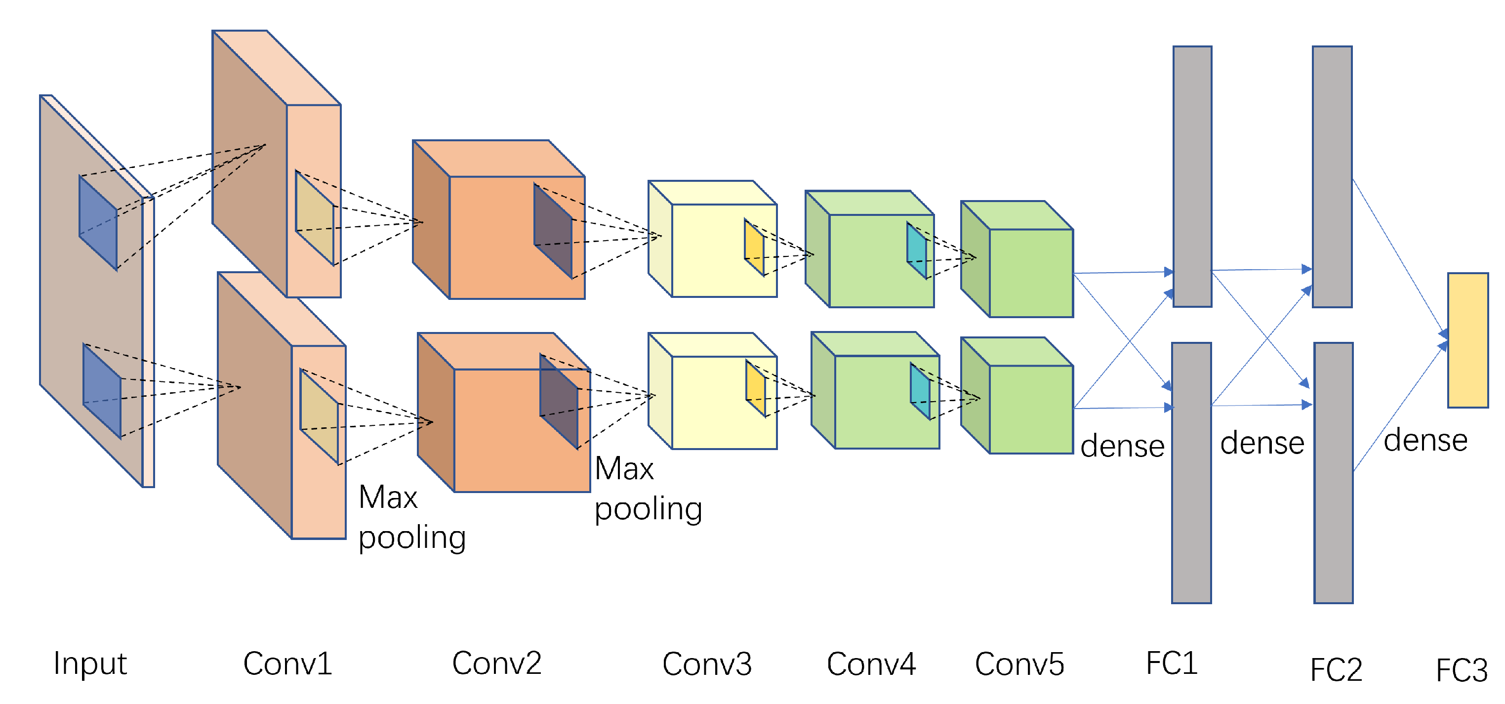
Convolutional Neural Networks (CNN) had outstanding advantages in handling two-dimensional input data. Therefore, the AlexNet network, proposed in 2012, was chosen for load recognition, as it represented a significant breakthrough in deep learning in the field of image recognition. The structure of this model consisted of 5 convolutional layers, 3 pooling layers, 2 Dropout layers, and 3 fully connected layers, with the activation function being Rectified Linear Units (ReLU). To accomplish the recognition task, the encoded VI trajectory image with filled background color was used as the model input (an

n \times n

matrix, where

n = 50

). The schematic diagram of the AlexNet network was shown in Figure 5.

The classic AlexNet network could not be directly applied to load recognition tasks and required some modifications to make it work properly. Additionally, due to the numerous hyperparameters, there was a need to optimize the hyperparameters of the convolutional layers, pooling layers, and fully connected layers in order to obtain a highly accurate recognition model.

4.3. Bayesian optimization algorithm

Bayesian Optimization (BO) was used to estimate the maximum value of a function based on existing sampled points when the functional equation was unknown [23]. It effectively addressed the classical problem of finding the next evaluation point based on acquired information about the unknown objective function to quickly search for the optimal solution [24]. Bayesian Optimization was highly applicable in evaluating costly and complex optimization problems and had been widely used in the optimization of machine learning hyperparameters, deep learning model hyperparameters, and other related areas. In this study, the hyperparameters selected for optimization were the number of convolutional kernels, size of convolutional kernels, stride of convolutional kernels, size of pooling kernels, stride, and Dropout probability. The optimization ranges were presented in Table 1. The parameter definitions for Bayesian Optimization were provided in Table 2.

5. Experimental analysis

5.1. Data set and evaluation criteria

This article validated the effectiveness of the algorithm using the PLAID dataset from Carnegie Mellon University in the United States. The dataset included instantaneous values of current and voltage for 11 different types of appliances, sampled at 30 kHz, recorded in multiple households in Pittsburgh, Pennsylvania. In this dataset, mixed currents with multiple loads were missing, and only individual current data when each load operated separately was available. Therefore, before analysis, it was necessary to align and superimpose the current values based on the voltage values to obtain mixed currents. This article selected 6 loads for load decomposition verification, namely, air conditioner, energy-saving lamp, laptop, vacuum cleaner, microwave oven, and washing machine.

5.2. Assessment of indicators

5.2.1. Evaluation indexes of decomposition process

In that section, root mean square error (RMSE), mean absolute error (MAE), phase error, and correlation coefficient were selected as the evaluation metrics. RMSE was a commonly used metric that measured the mean square difference between predicted and actual values, representing the average magnitude of prediction errors. A lower RMSE value indicated that the predicted results were closer to the actual values. MAE was another common evaluation metric that measured the average absolute difference between predicted and actual values, reflecting the absolute error of the predictions. Phase error was an important metric for high-frequency current decomposition, measuring the error between the predicted and actual phase of the signals. Correlation coefficient was used to measure the linear correlation between predicted and actual values. A correlation coefficient closer to 1 indicated a better linear relationship between the predictions and the actual values. The definitions of these four evaluation metrics were as follows:

R M S E = \sqrt{\frac{1}{n} \sum_{i = 1}^{n} {(I_{i} - {\hat{I}}_{i})}^{2}}

(18)

M A E = \frac{1}{n} \sum_{i = 1}^{n} |I_{i} - {\hat{I}}_{i}|

(19)

P h a s e E r r o r = arccos (\frac{\sum_{i = 1}^{n} I_{i} {\hat{I}}_{i}}{\sqrt{\sum_{i = 1}^{n} I_{i}^{2} \sum_{i = 1}^{n} {\hat{I}}_{i}^{2}}})

(20)

C o r r e l a t i o n = \frac{\sum_{i = 1}^{n} (I_{i} - \bar{I}) ({\hat{I}}_{i} - \bar{\hat{I}})}{\sqrt{\sum_{i = 1}^{n} {(I_{i} - \bar{I})}^{2} \sum_{i = 1}^{n} {(\hat{I_{i}} - \bar{\hat{I}})}^{2}}}

(21)

5.2.2. Evaluation metrics for load recognition process

In the evaluation of non-intrusive load identification performance, the paper mainly used common evaluation metrics such as recognition accuracy (accuracy, Acc),

F 1

score, and F-measure [25] as the evaluation standards for the identification model. The calculation formulas were shown in Equations 22 to 25.

A c c = \frac{m}{n}

(22)

where m denoted the number of correct classifications of the model, and n was the total number of samples.

F_{1_{i}} = 2 \cdot \frac{p r e c i s i o n_{i} \cdot r e c a l l_{i}}{p r e c i s i o n_{i} + r e c a l l_{i}}

(23)

p r e c i s i o n_{i} = \frac{T P_{i}}{T P_{i} + F P_{i}}

(24)

r e c a l l_{i} = \frac{T P_{i}}{T P_{i} + F N_{i}}

(25)

In the equation:

T P

represented the count of true positive, where both the true value and the predicted value were positive;

F P

represented the count of false positive, where the true value was negative but the predicted value was positive;

F N

represented the count of false negative, where the true value was positive but the predicted value was negative. The following equation could obtain the average value for each device:

F_{i_m e a n} = \frac{1}{L} \sum_{g = 1}^{L} F_{g_i}

(26)

In the equation: L represented the total occurrences of device i in the test set;

F_{g_i}

represented the F-measure value of device i in the gth occurrence. Finally, by calculating the average of all F-measures using Equation 26, we obtained the macro-average value

F_{m a c r o}

F_{m a c r o} = \frac{1}{A} \sum_{i = 1}^{A} F_{i_m e a n}

(27)

where A was the total number of different equipment types.

5.3. Example analysis

5.3.1. Load decomposition

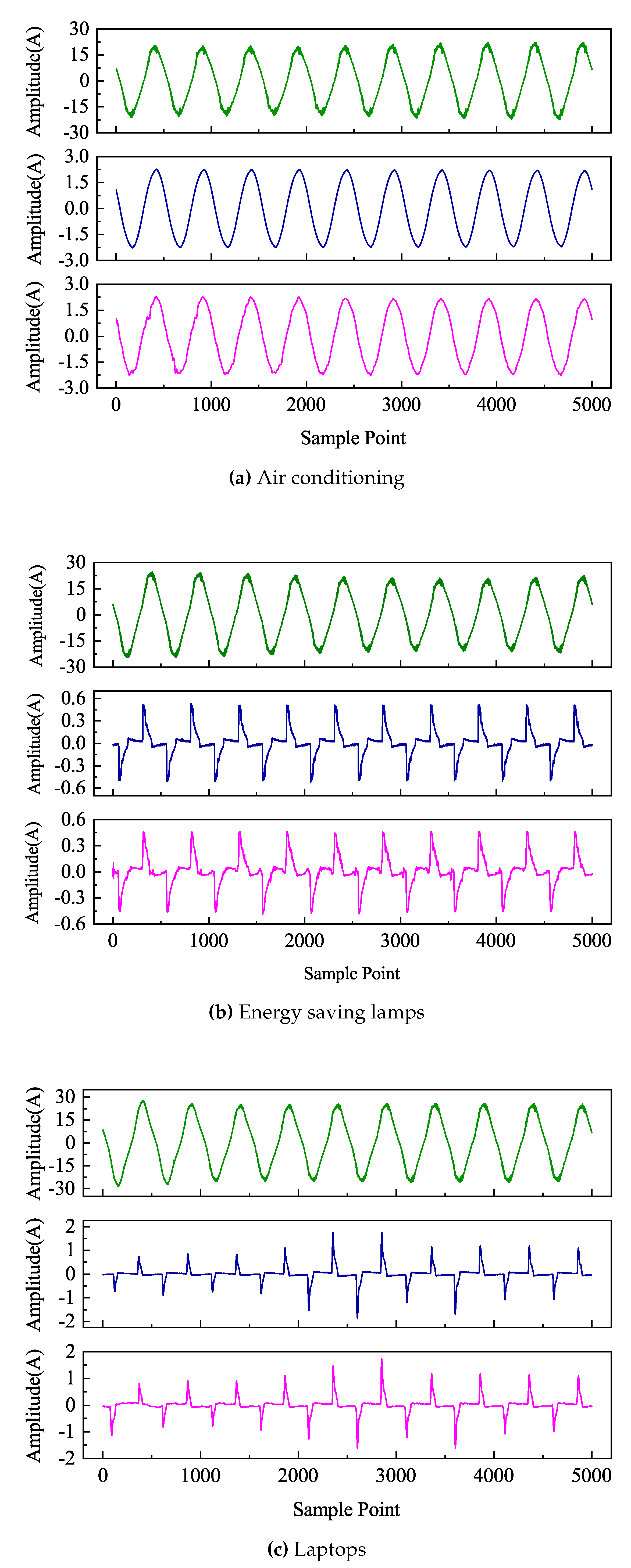
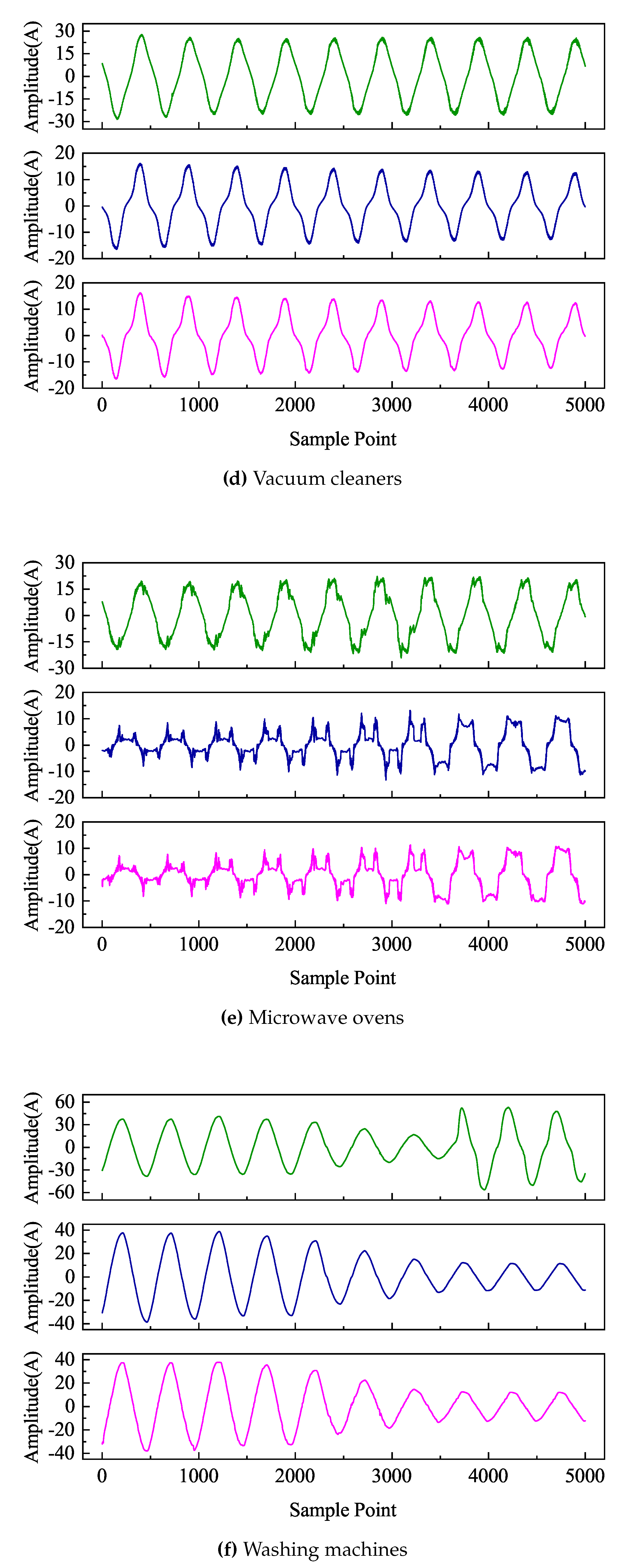
The input of the LSTM-DAE model was a mixed current obtained by superimposing multiple load currents. The window size of the data input was set to 10 cycles of current data; in the PLAID dataset, one cycle contained 500 data points. Therefore, the size of each window was set to 5000. The sliding step was one cycle of data, which was 500 data points. The training times (epochs) were set to 1000. The decomposition results were shown in Figure 6. Each figure contained three curves, from top to bottom representing the mixed current, the true target load current, and the predicted target load current.

Figure 6. Monochromatic VI trajectory, VI trajectory with color coding and color coded VI trajectory with background colors(part 2).

From the Figure 6, it could be seen that using the LSTM-DAE network model effectively extracted the latent information of strongly correlated current sequences and mined the temporal features within the time series signals. Even in cases where mixed signals and actual signals exhibited irregular variations, the model accurately decomposed the target signal. Overall, the decomposed current signals output by this model were able to track the variations of actual current signals well and essentially fit the rising and falling trends of actual current curves. These results indicated that the model performed well in the decomposition and fitting of current signals.

From the Table 3, it could be seen that out of the 6 types of loads, 5 of them had correlation coefficients exceeding 98%. Even the load with the lowest correlation coefficient, which belonged to the laptop category, had a coefficient close to 95%. This indicated a strong linear relationship between the predicted results of the algorithm and the actual values, effectively capturing the changing trends of load current. Additionally, the maximum values for RESE, MAE, and Phase Error were 0.866, 0.551, and 0.332 respectively. In comparison to the 4 network models listed in Reference [29], the algorithm in this study achieved a minimum MAE score of 5.97 and a minimum RMSE of 10.52, demonstrating a significant improvement in algorithm performance. Overall, the algorithm exhibited high precision, low phase error, and strong correlation in current signal decomposition tasks, making it particularly suitable for handling high-frequency currents. These advantages gave the algorithm potentially high practical value in applications such as power load analysis and energy management, providing a reliable tool.

5.3.2. Load Recognition

After converting the dataset into VI trajectory images with background color coding, it was input into the CNN network, and the Bayesian optimization algorithm was used to optimize the hyperparameters of the convolutional layers, pooling layers, and Dropout layers. There were a total of 5 convolutional layers, 3 pooling layers, and 2 Dropout layers. The comparison of hyperparameters before and after optimization was shown in Table 4. The data in the table indicated, for example, that the parameters of Conv1 layer were 3*3/48/1, which meant the convolutional kernel size was 3*3, the number of convolutional kernels was 48, and the stride was 1. The parameter of Dropout1 layer was 0.5, indicating a Dropout probability of 0.5.

While validating the accuracy of the optimized model, it was compared with the recognition accuracy in other literature, as shown in Table 5. The accuracy of the CNN network optimized by Bayesian optimization was approximately 96.5%, while the accuracy of the regular CNN network was approximately 93.1%, indicating a 3.4% improvement. Compared to other models, the recognition accuracy was also higher.

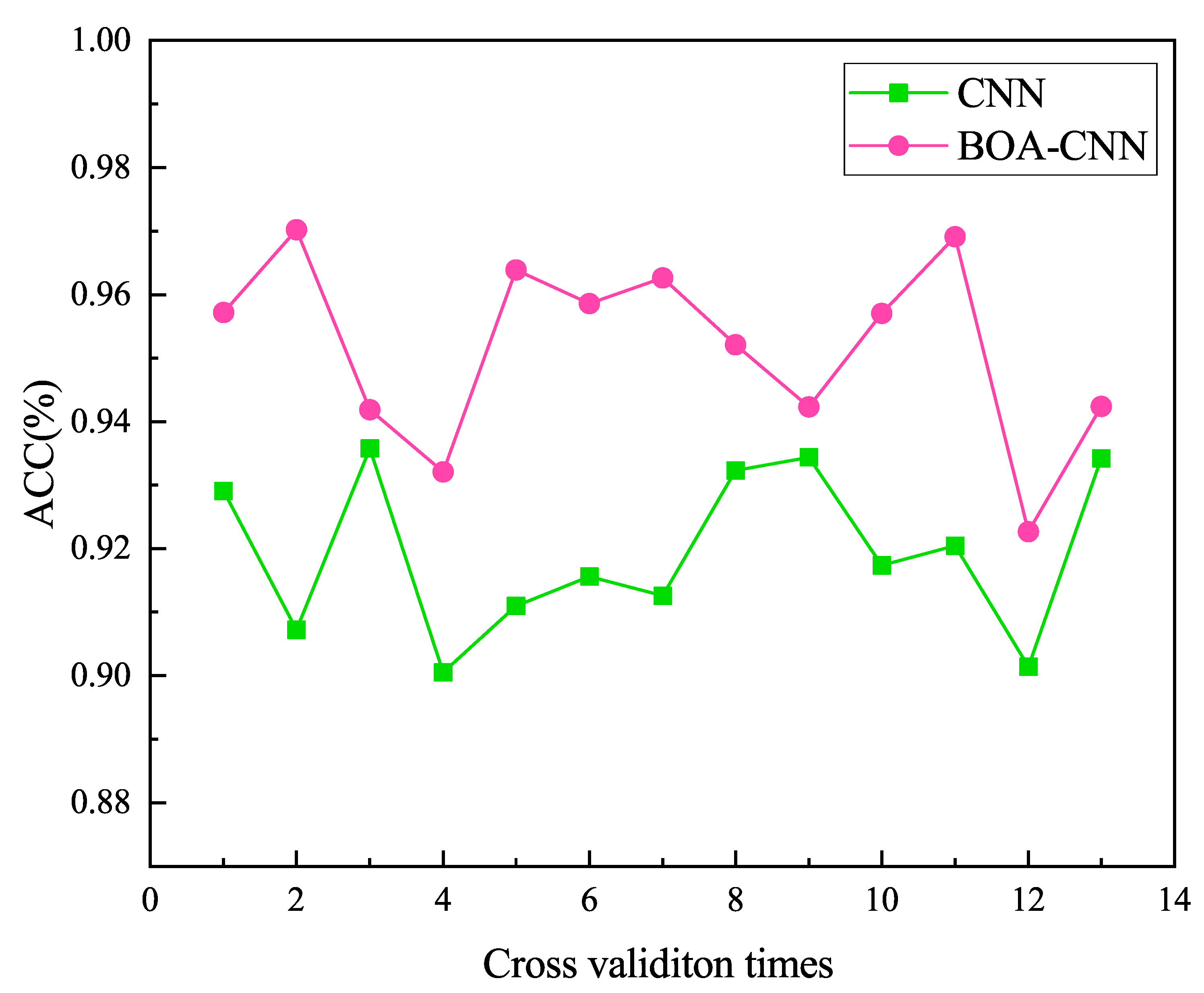
In order to test the stability of the BOA-CNN algorithm, 12 experiments were conducted on the PLAID dataset to verify the stability. As shown in Figure 7, the recognition accuracy of the BOA-CNN algorithm is superior to that of the ordinary CNN model in all experiments, with good robustness. However, in terms of stability, the BOA-CNN algorithm performs poorly and fluctuates significantly. Specifically, in 12 experiments, the difference between the maximum and minimum accuracy of the BOA-CNN algorithm is about 4.7%, while the difference between the ordinary CNN model is about 3.5%. This indicates that the BOA-CNN algorithm is unstable in different experiments. Further analysis shows that this instability may be caused by the randomness and local optimal solution of Bayesian optimization algorithms. However, its automatic search for the optimal hyperparameters of the convolution layer, pooling layer, and Dropout layer reduces the time and labor costs of manual parameter adjustment.

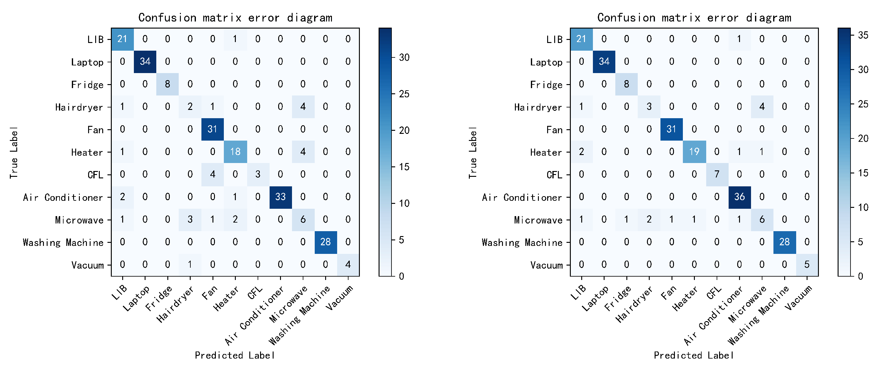
The model confusion matrix is shown in Figure 8, where the number in each cell represents the number of corresponding devices, the abscissa represents the predicted value of the appliance, and the ordinate represents the actual value of the appliance. It can be seen that in the PLAID dataset, compared to the ordinary CNN model, the BOA-CNN model reduces the number of false negative (

F N

) and false positive (

F P

) for each electrical appliance, and also reduces the number of device types that are incorrectly classified for each electrical appliance. This indicates that the BOA-CNN model has shown excellent results in the accuracy of electrical identification, and has practical value.

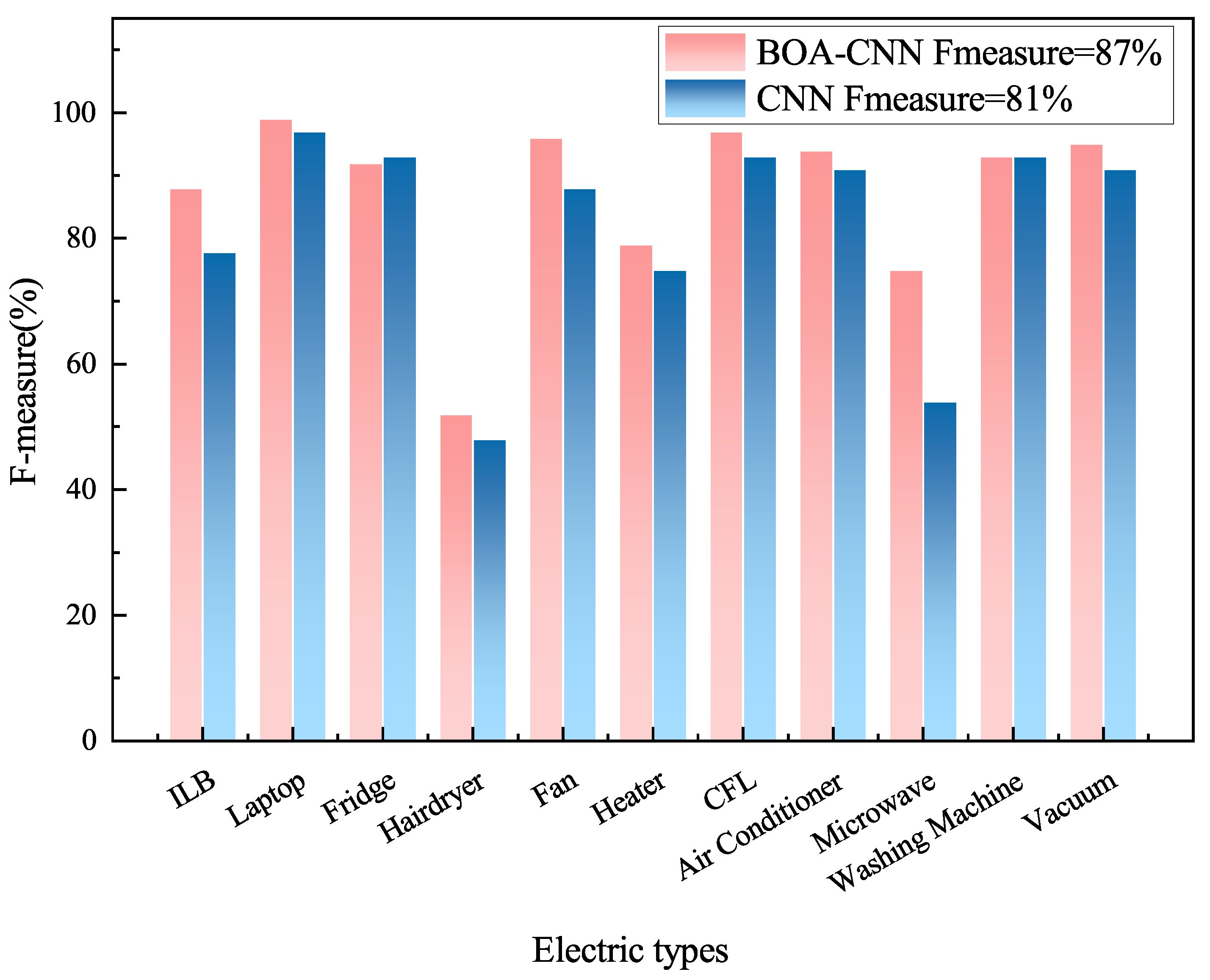
For F-measure indicators and

F_{m a c r o}

indicators, as shown in Figure 9, the

F_{m a c r o}

indicator for BOA-CNN is 87%, while the

F_{m a c r o}

indicator for CNN is 81%. In addition, F-measure values for hair dryers is lower than the macro average. This may be due to the small amount of measurement data for some devices in the dataset, which limits the learning ability of the model, resulting in lower F-measure values for some devices. However, in general, the convolutional neural network model based on Bayesian optimization proposed in this paper has improved compared to the original convolutional neural network model for 11 types of electrical appliances in the PLAID dataset, with a maximum improvement of 21%. Therefore, the model has good performance.

6. Summarize

This article proposed a load decomposition method based on LSTM-DAE, as well as a load recognition method that utilized color encoding of VI trajectories with background color filling. The results of a case study showed that the proposed load decomposition method achieved an accuracy of over 98% and exhibited a good current reproduction effect, providing accurate data support for high-frequency load recognition. By integrating multi-period signals, color encoding of VI trajectories, and background color filling, the method increased the differentiation between different load VI trajectories. Furthermore, by using the BOA-optimized Alexnet network to recognize VI trajectories, experimental results indicated that the BOA-CNN model effectively reduced confusion between devices and demonstrated high accuracy and robustness. Compared to traditional CNN models, this method performed better in various appliance recognition performance metrics.

References

Yang, X.; Zhou, M.; Li, G. Survey ondemand response mechanism and modeling in smart grid. Power System Technology 2016 , 40, 220–226.
Qi, B.; Liu, L.; Han, L.; et al. Home appliance load identification algorithm based on system model. Electrical Measurement & Instrumentation2018 , 55, 23–30.
Zhang, G.; Wei, Q.; et al. A survey on the non-intrusive load monitoring. Acta Automatica Sinica2022 , 48, 644–663.
Li, P. Non-intrusive method for power load disaggregation and monitoring. Master, Tianjin University, Tianjin, China, 2009.
Liu, Y .; Qiu, J.; Ma, J. SAMNet: Toward Latency-Free Non-Intrusive Load Monitoring via Multi-Task Deep Learning. IEEE Transactions on Smart Grid2022 , 13, 2412–2424. [CrossRef]
Kim, H.; Marwah, M.; Arlitt, M.; et al. Unsupervised Disaggregation of Low Frequency Power Measurements. Proceedings of the 2011 SIAM International Conference on Data Mining, SIAM, 2011.
Kolter, Z.; Jaakkola, T.; Kolter, J. Z. Approximate Inference in Additive Factorial HMMs with Application to Energy Disaggregation. Journal of Machine Learning Research2012 , 22, 1472–1482.
Li, D.; Li, J.; Zeng, X.; et. al. Transfer learning for multi-objective non-intrusive load monitoring in smart building. Applied Energy2023 , 329, 1472–1482. [CrossRef]
Kim, H.; Marwah, M.; Arlitt, M.; et.al. Neural NILM: Deep Neural Networks Applied to Energy Disaggregation. ACM International Conference on Embedded Systems for Energy Efficient Built Environments BuildSys, Seoul, Korea, Republic of, November 4, 2015.
Roberto, B.; Felicetti, A.; Principi, E. Denoising Autoencoders for Non-Intrusive Load Monitoring: Improvements and Comparative Evaluation. Energy and Buildings2018 , 158, 1461–1474.
Odysseas, K.; Christoforos, N.; Dimitris, V. Sliding Window Approach for Online Energy Disaggregation Using Artificial Neural Networks. 10th Hellenic Conference on Artificial Intelligence, Patras, Greece, July 9, 2018.
Zhang, C.; Zhong, M.; Wang, Z.; et.al. Sequence-To-Point Learning with Neural Networks for non-intrusive Load Monitoring. non-intrusive, non-intrusive, July 9, 2018, February 2, 2018.
Xu, X.; Zhao, S.; Cui, K. Non-intrusive load decomposition algorithm based on convolution block attention model. Power System Technology2021 , 45, 3700–3705.
Piccialli, V,; Sudoso, A. Improving Non-Intrusive Load Disaggregation through an Attention-Based Deep Neural Network. Energies2021 , 41.
Piccialli, V,; Sudoso, A.A nonintrusive recognition method of household load behavior based on DTW algorithm. Electrical Measurement & Instrumentation2019 , 56, 17–22.
Zhu, H.; Cao, N,; Lu, H.; et al. Non-intrusive load identification method based on feature weighted KNN. Electronic Measurement Technology2022 , 56, 70–75.
Dong, Z.; Chen, Y.; Xue, T.; et al. Non-intrusive load monitoring algorithm based on attention mechanism combined with global and sliding window. Electrical Measurement & Instrumentation2021, 1–8.
Yu, D.; Liu, M. A non-invasive load decomposiontion method base on deep circular convolutional model. Electrical Measurement & Instrumentation2020, 57, 47–53.
Lam, H.Y.; Fung, G.S.K.; Lee, W.K. A novel method to construct taxonomy electrical appliances based on load signatures. IEEE Transactions on Consumer Electronics2007, 53, 653–660. [CrossRef]
Bates, L. D.; Develder, C.; Dhaene, T.; et al. Automated classification of appliances using elliptical fourier descriptors. 2017 IEEE International Conference on Smart Grid Communications, Dresden, Germany, October 23, 2017.
Hassan, T.; Javed, F.; Arshad, N. An Empirical Investigation of VI Trajectory Based Load Signatures for Non-Intrusive Load Monitoring. IEEE Transactions on Smart Grid2014, 5, 870–878. [CrossRef]
Vincent, P.; Larochelle, H.; Bengio, Y.; et al. A Extracting and composing robust features with denoising autoencoders. 25th International Conference on Machine Learning, Helsinki, Finland, July 5, 2008.
Zhu, H.; Liu, X.; Liu, Y. Bayesian-based novel deep learning hyperparameter optimization. Data Communications2019, 2, 35–38.
Jones, D.; Schonlau, M.; Welch, W. Bayesian-based novel deep learning hyperparameter optimization. Journal of Global Optimization1998, 13, 455–492. [CrossRef]
Yu, X.; Xu, L.; Li, J.; et al. MagConv: Mask-Guided Convolution for Image Inpainting.IEEE Transactions on Image Processing2023, 32, 4716–4727. [CrossRef] [PubMed]
Zheng, Z.; Chen, H.; Luo, X. A supervised event based non-intrusive load monitoring for non-linear appliances.Sustainability2018, 10. [CrossRef]
De Baters, L.; Develder, C.; Dhaene, T.; et al. Automated classification of appliances using elliptical fourier descriptors. 2017 IEEE International Conference on Smart Grid Communications, Dresden, Germany, October 23, 2017.
Gao, J.; Kara, E.; Giri, S.; et al. A feasibility study of automated plug-load identification from high-frequency measurements. IEEE Global Conference on Signal and Information Processing, Orlando, FL, United states, December 13, 2015.
Cui, H. Non-intrusive load monitoring and decomposition technology based on deep learning and application of typical scenarios. Master, Northeast Electric Power University, Dalian, China, 2023.

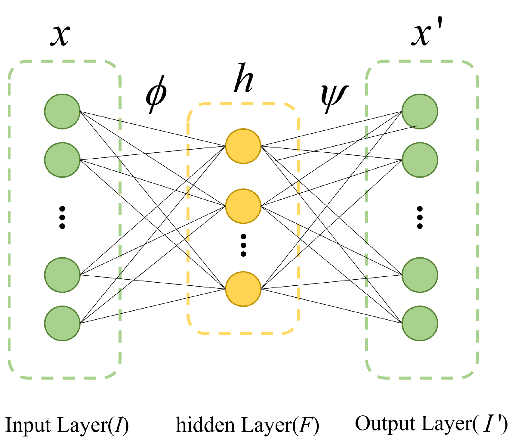
Figure 1. Basic structure of Autoencoder.

Figure 2. Structure of Denoising Autoencoder.

Figure 3. Structure of Denoising Autoencoder.

Figure 4. Monochromatic VI trajectory, VI trajectory with color coding and color coded VI trajectory with background colors.

Figure 5. AlexNet network model diagram.

Figure 7. Comparison of recognition accuracy between BOA-CNN and CNN.

Figure 8. Comparison of BOA-CNN and CNN confusion matrices.

Figure 9. Comparison between BOA-CNN and CNNF-measure indicators and Fmacro indicators.

Table 1. Hyperparameters to be optimized and their ranges.

Layers	Hyperparameters	Dynamic range
	Number of convolution kernels	30 ∼ 135
Conv	Convolution kernels size	2 ∼ 6
	Convolution kernels step	1 ∼ 3
Pool	Pool core size	2 ∼ 6
	Pool nucleation step size	1 ∼ 3
Dropout	Dropout rate	0 ∼ 1

Table 2. Parameter Definition in Bayesian Optimization Algorithms.

Layers	Hyperparameters
a1,a2,a3,a4,a5	The number of convolution kernels in five convolutional layers
b1,b2,b3,b4,b5	Convolutional kernel size for five convolutional layers
c1,c2,c3,c4,c5	Convolutional kernel step size for five convolution layers
d1,d2,d3	The number of pooling kernels in the three pooling layers
e1,e2,e3	Step size of pooling kernels in three pooling layers
f1,f2	Dropout rate of the two layers

Table 3. Evaluation metrics scores of the LATM-DAE algorithm.

Load Type	RMSE	MAE	Phase Error	Correlation Coefficient(%)
Air conditioner	0.109	0.081	0.068	99.8
Energy-saving lamps	0.033	0.020	0.196	98.1
Notebook	0.097	0.040	0.332	94.5
Vacuum cleaner	0.295	0.220	0.035	99.9
Microwave Oven	0.668	0.456	0.129	99.2
Washing Machines	0.866	0.551	0.046	99.9

Table 4. Comparison of super parameter information between CNN and BOA-CNN.

Catagory	CNN	BOA-CNN
Conv1	3×3/48/1	4×4/60/1
Pool1	3×3/2	2×2/1
Conv2	5×5/128/2	4×4/121/1
Pool2	3×3/2	2×2/1
Conv3	3×3/192/1	4×4/126/1
Conv4	3×3/192/1	3×3/55/1
Conv5	3×3/192/1	3×3/125/1
Droout1	0.5	0.4
Droout1	0.5	0.1

Table 5. Comparison of recognition accuracy of various algorithms.

Model	accuracy(%)
BOA-CNN	96.5%
CNN	93.1%
Literature [26]	80.7%
Literature [27]	79.4%
Literature [28]	82.4%

Disclaimer/Publisher’s Note: The statements, opinions and data contained in all publications are solely those of the individual author(s) and contributor(s) and not of MDPI and/or the editor(s). MDPI and/or the editor(s) disclaim responsibility for any injury to people or property resulting from any ideas, methods, instructions or products referred to in the content.

© 2023 by the authors. Licensee MDPI, Basel, Switzerland. This article is an open access article distributed under the terms and conditions of the Creative Commons Attribution (CC BY) license (http://creativecommons.org/licenses/by/4.0/).

Copyright: This open access article is published under a Creative Commons CC BY 4.0 license, which permit the free download, distribution, and reuse, provided that the author and preprint are cited in any reuse.

MDPI Initiatives

Important Links

Choose an area of interest and we will send you notifications of new preprints at your preferred frequency.

Disclaimer

Research on Non-intrusive Load Recognition Algorithm Based on High Frequency Signal Decomposition with Improved VI Trajectory and Background Color Coding

Abstract

1. Introduction

2. Related works

3. LSTM-DAE based load decomposition

3.1. Load decomposition

3.2. Denoising Autoencoder

3.3. Decomposition model based on LSTM-DAE

4. Load recognition of VI traces based on background color coding

4.1. Construction of VI trajectory pixelization

4.2. Construction of convolutional neural network

4.3. Bayesian optimization algorithm

5. Experimental analysis

5.1. Data set and evaluation criteria

5.2. Assessment of indicators

5.2.1. Evaluation indexes of decomposition process

5.2.2. Evaluation metrics for load recognition process

5.3. Example analysis

5.3.1. Load decomposition

5.3.2. Load Recognition

6. Summarize

References

MDPI Initiatives

Important Links

Subscribe