Submitted:
10 November 2023
Posted:
13 November 2023
Read the latest preprint version here
Abstract
Hubble diagrams are examined for SN1a supernovae in the redshift range z = 0.01–1.3 and for gamma ray bursts in the range z = 0.034–8.1. It is shown that in the low redshift range, the Hubble diagram shows an innate equivocality between the ΛCDM and the tired light model. This means that the strong agreement between the z/µ data, calculated with the parameters of the ΛCDM model, and the experimentally measured z/µ values cannot be considered as definite evidence for the expansion hypothesis. The exponential function , which is characteristic of the tired light redshift mechanism, fits the data with similarly high accuracy. Hence, on the premise of low redshift data, a decision for or against either model is completely arbitrary. The Hubble diagram for high redshift gamma ray bursts shows poor agreement with the ΛCDM model, but concurs with the exponential energy decay following from the tired light redshift hypothesis.
Keywords:
galaxies
; distances and redshifts - galaxies
; high-redshift - stars
; gamma ray burst
; general - cosmology
; cosmological parameters
1. Introduction
The essential premise of Big Bang (BB) cosmology is that the universe is expanding, and Hubble's law (Hubble 1929) is viewed as the most persuasive proof for cosmic expansion. In present-day cosmology, the velocity interpretation of the redshift (RS) of spectral lines has achieved a dogmatic status, and objections against it have gone unobserved.
Regardless of whether this interpretation is correct or not, Hubble’s law is a RS/distance (d) relation, and an interpretation of this as a velocity is only a hypothesis. Supporting the velocity interpretation is the good agreement between the observed z/µ data for SN1a supernovae in the RS range z < ~ 1.3 with data determined based on the parameters ΏM, Ώλ, w and H0 of the ΛCDM model, which is viewed as proof for general expansion. Despite its widespread acceptance, however, this conclusion is equivocal, and the current circumstance is fairly confounding. Based on a semiquantitative examination of SN1a data, Sorell (2009) reported that in the low-RS range, the Hubble diagram (HD) for a tired light (TL) cosmology gives good agreement with the Type Ia supernova data. A detailed examination of mixed SN1a and gamma ray burst (GRB) data (Marosi 2013) has also shown that in the RS range 0.031–8.1, the TL model (Zwicky 1932) closely fits the experimental data, while the ΛCDM model is in poor agreement with observation. A comparable outcome was described by Traunmüller (2014), whose examination of 892 SN1a supernovae z/µ data also indicated that these were well-matched with the TL model.
The interpretation of the RS of atomic spectral lines suffers from the fact that none of the proposed systems (the expanding space paradigm or the TL mechanism) can be confirmed experimentally, meaning that confidence in each hypothesis should be estimated based on its ability to explain the observational data. One important issue in cosmology is therefore to explain which of the two models fits the observed data better, i.e., whether the HD follows the linear (expanding universe) or the exponential TL relation. In the high RS range, it should be more feasible to check more precisely whether the HD follows a linear or exponential slope.
Very exact z/μ data for SN1a supernovae, however, are accessible only for a limited range of distances. At RS > ~ 1.3, the optical light emitted by a supernova gradually diminishes with distance, making definite estimations difficult. Hence, some attempts have been made to collect and use GRB data for computing HDs in the high RS range (Schäfer 2003, 2006, Wei 2010, Amati 2018).
Using mixed SN1a and GRB or exclusively GRB data, Marosi (2014, 2016, 2019) observed that the slope of the HD is (or is extremely close to) exponential, which is characteristic of the TL model. In contrast, ongoing investigations by Gupta (2019) and Shirokov et al. (2020a, 2020b) have found that although none of the existing studies has given probative affirmation for the ΛCDM model, the conclusion can be drawn that based on the HD test, the TL model can be precluded. This cosmologically significant inconsistency between these two contradictory conclusions requires an amendment.
2. Aims
The HD test represents possibly the most significant proof for identifying the underlying physical nature of the Hubble constant (abbreviated as hCDM = (km s-1 Mpc-1)/100 for ΛCDM and hTL = (Hz s-1 Hz-1)/100 for the TL model), and could provide solid support for the expansion hypothesis, or, in the contrary case, for the legitimacy of the TL model (although this would require modification to the ΛCDM itself).
The aim of the present study was to perform a comparative HD test using cosmology-independent SN1a data and high RS GRB RS/μ data. Since both the ΛCDM and the TL model make precise forecasts about the shape of the HD, it ought to be possible to confirm whether the HD shows a linear
or exponential relationship
(where t represents the flight time of the photons from the co-moving radial distance d to the observer; for simplicity, we will use t instead of d in the following discussion). This could set significant constraints on these contrasting cosmological models.
We do not plan to examine existing issues related to the ΛCDM and TL cosmology, or to accept or reject either model on the basis of hypothetical contentions or hypotheses. The present study is completely cosmology-independent; it is a mathematically based statistical investigation based on cosmology-independent data without the need to turn to cosmological suspicions, meaning that it is unbiased.
3. Datasets and methods
3.1. SN1a supernovae
(a) For the model calculations, the cosmological parameters ΏM = 0.295, Ώλ = 0.705, w = −1.018 and h0 = 0.7 were used, based on 374 spectroscopically affirmed, upgraded SN1a supernovae from the most recent joint light-curve analysis (JLA) data index (Betoule et al. 2014).
3.2. Choice of GRB data
(b) 60 low RS and 78 high RS GRB data samples from the Union1 compilation, collected by Liu and Wei (2015). One extreme outlier at ln(z+1) = 1.2095 with t = 17491×10-14 was excluded from the calculation.
(c) 193 GRB data samples collected by Amati et al. (2018).
(d) 134 GRB data samples (Demianski et al. 2017).
A comparison of the goodness of fit indicators for data sets b), c) and d) is shown in Table 1.
Based on the above quality criteria, we selected 138 calibrated, cosmology-independent GRB data points in the RS range z = 0.0331–8.1 for a detailed analysis.
4. Data processing
Data were introduced on the usual, strongly attenuated logarithmic z/μ scale, and since the contrast between the measured and the modelled data turned out to be clearer on the linear scale, we also considered the less commonly used but more sensitive linear photon flight time t/(z+1) scale. A conspicuous benefit of the t/(z +1) representation is the direct illustration of the shape of the HD, which can be definitively contrasted with the expectations following from Equations (1) and (2).
4.1 Data conversion from µ to t(d) and vice versa
For data conversion from µ to t we used Equation (3), and for conversion from t to µ we used Equations (4) and (5), as follows:
Conversion of the SN1a µ data to a linear scale was straightforward, as the data were of high precision and Equation (3) could directly be applied for conversion without producing disruptive amplification of measurement errors.
Due to experimental difficulties in determining z/μ data at high RS, these data were overwhelmed by substantial scatter, meaning that they could not be converted to the linear t/(z +1) scale without amplifying the scatter and making the converted data unmanageable. Hence, before data conversion, there was a need to either smooth the data scatter by calculating the line of best fit using a suitable arithmetical function or to multiply the t values by an appropriate damping factor, which in this case was selected as 10-14. For data fitting, a third-order polynomial regression was used.
4.2. Goodness of fit
The goodness of fit was calculated using the likelihood estimator
4.3. Calculations of RS/µ data
For the ΔCDM model, the ICRAR cosmology calculator was used to calculate the theoretical z/µ data. For the TL models, the z/µ data were calculated as follows:
(see: Sorrell 2009; Vigoureux, Vigoureux & Langlois 2014; Traunmüller 2014).
4.4. Data presentation
Excel was used for data fitting, refinement, and presentation.
5. Results
5.1. Equivocality of the SN1a supernovae Hubble diagram
Since for ΛCDM models the distances in Equation (1) are nonlinear in z (the distances are limited by the maximum value for d, i.e., the radius of the universe), it is usual to express d as  . This leads to a linear relationship for the variables
which are the usual coordinates for the graphical presentation of the HD.
. This leads to a linear relationship for the variables
which are the usual coordinates for the graphical presentation of the HD.
. This leads to a linear relationship for the variables
For TL models, it follows from Equation (2) that
which is linear with distance, with an intercept on zero.
ln (z + 1) = hTL × t
Figure 1 shows the HD calculated with the parameters of the ΛCDM model, as set down by Betoule et al. (2014), in the RS range z = 0.01–1.35 for the log(z)/µ presentation. Figure 2 shows the same data plotted on the ln(z+1)/t scale.
As illustrated by Figure 1 and Figure 2, both Equation (8) (the expanding universe model) and Equation (9) (the TL model) match the calculated data with very high accuracy. The exceptionally small ∑χ2 values on the order of 10-5–10-6 offer convincing evidence of the equivocality of the ΛCDM and TL model in the low RS range.
The corresponding linear t/(z+1) HDs were derived by converting µ to t using Equations (3-5) based on the fit coefficients from Equations (8) and (9). The linear HDs for both the log(z) and the ln(z+1) representations and the linear HD for the calculated data are shown in Figure 3.
The three curves (i.e., the one calculated based on the parameters of the ΛCDM model, and the log(z)/µ and d/ln(z+1) lines) have an exponential slope, are closely congruent, and cannot be told apart by visual examination. The corresponding Hubble constants and variances are shown in Table 4.
The Hubble constants are similar to within 0.5%, with values of hTL = 0.6319 for the logarithmic log(z)/µ fit and 0.6322 for the ln(z+1) fit and calculated data.
Based on model calculations using 35 equidistant data points in the RS range z = 0.03–1.02, the hTL equivalents for hCDM = 0.68, 0.70 and 0.73 were determined in a similar way. The results are summarised in Table 5.
An obvious but frequently overlooked outcome is that, as shown in Table 5, the equivalent Hubble constants hCDM and hTL are different, and this has a significant effect on the comparative evaluation of the ΛCDM and TL models in the high RS range. It can be seen from Table 6 that the comparison of the observed high RS GRB data with the competing ΛCDM and TL models using hCDM = hTL is imprecise.
The ∑χ2 differences between hCDM = 0.70 and hTL = 0.70 for the observed data show that hTL = 0.70 gives the poorest fit, whereas a comparison of hCDM = 0.70 with hTL = 0.66 shows the opposite: the hTL = 0.66 model gives the best fit to the observed data. The use of hTL = hCDM instead of the best fit hTL for comparison inevitably leads to the wrong conclusion, that the TL model does not fit the data and can therefore be rejected. The results presented here show that for a proper comparison of ∑χ2 for TL models, the correct approach is a Hubble constant close to the expectation value of hTL, as shown in Table 5, or, depending on data quality (influence of scatter and/or outliers on χ2), the best-fit value of hTL.
6. Hubble diagram for high RS GRBs
6.1. log(z)/µ Hubble diagram
As the data points for high RS show pronounced scatter, the variance of the fit reaches only R2 = 0.8746, and cannot be improved by any other reasonable mathematical function. The fit coefficients are shown in Table 7.
Figure 5 shows the linear t/(z+1) HDs inferred from the best fit coefficients of the observed data (squares) together with the corresponding exponential hTL = 0.66 (dots) and the HD for hCDM = 0.70 (triangles).
The GRB HD exhibits some irregular shape between hTL = 0.66 and hCDM = 0.7 with
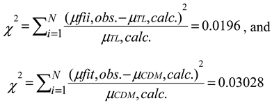
(µfit,obs stands for calculated magnitudes inferred from the polynomial best-fit function, µTl calc. and µCDM calc. were calculated from hTL = 0.66 for the TL and from ΏM = 0.287, w = -1 and hCDM = 0.7 for the ΔCDM model, respectively.)
The result favours the TL model, but as can be seen from Figure 5, the deviation from the ideal exponential shape is too large to draw safe conclusions. A profile examination shows systematic deviations, especially at RS ≥ ~ 3–4, where data points are visible above the exponential line.
In summary, the ΔCDM model shows a poorer fit to the HD calculated on the basis of observed data, which suggests a somewhat better but still not correct portrayal of the TL model. No safe conclusion in favour of or against either of the competing models can be drawn from this result.
6.2. ln(z+1)/t Hubble diagram
Despite the extensive scatter in the observed photon flight times even at values of z ≥ ~ 1.4, the ln(z+1)/t diagram is linear. Considering the quality of the data, it shows an astonishingly good variance of R2 = 0.8447 that could only be worsened by fitting the observed data with higher-order polynomials. From Figure 6, the equation that describes the photon flight time/z relationship on the t×10-14 scale that goes into the linear t/(z+1) diagram is
t = 4897 × ln (z + 1)
The linear HD has a perfect exponential slope, with hTL = 0.63. This is in exceptionally good agreement with the expected value of hTL = 0.632 obtained from model calculations, although it is in clear conflict with the presently accepted point of view that the TL model does not fit the observed RS/µ data. The conclusion from the outcome of the ln(z+1) t-test is that both the low RS SN1a data and the high RS GRB HDs for a TL cosmology give an adequately good fit to the observed data. From an unbiased examination of the data, we see that the TL model cannot be dismissed from further consideration.
7. Conclusion
The most remarkable outcome of the HD test introduced in this analysis is that in the low RS range between z = 0.01–1.3, the HD is equivocal and permits no distinction based on the data between the ΛCDM and TL model. The HD can be equally well described with the parameter of the ΛCDM model as with the exponential function  .
.
.In the high RS range up to z = 8.1, the observed z/µ data conflict with the ΛCDM, and favour the TL model. This result raises serious questions about the legitimacy of the concordance model. For definite proof, more exact and numerous data are needed, particularly in the high RS range, to confirm or reject this cosmologically significant result. The key question of the real shape of the HD, as predicted by the ΛCDM or exponential model, cannot be seen as settled, but it is no way justified to exclude the TL model from further consideration.
Funding
No funding was acquired for this research.
Data Availability Statement
The author confirms that the data supporting the findings of this study are available within the article and the reference list.
Conflicts of Interest
The author declares no conflict of interest.
References
- Amati L., D’Agostino R., Luongo O., Muccino M., Tantalo M., 2018, Addressing the circularity problem in the Ep−Eiso correlation of gamma-ray bursts, arXiv:1811.08934 [astro-ph HE]. [CrossRef]
- Betoule M. et al., 2014, Improved cosmological constraints from a joint analysis of the SDSS-II and SNLS supernova samples, arXiv:1401.4064, [astro-ph-CO]. [CrossRef]
- Demianski M., Piedipalumbo E., Sawant D., & Amati L., 2017, Cosmology with gamma-ray bursts, I. The Hubble diagram through the calibrated Ep,i–Eiso correlation, A&A, 598, A112. [CrossRef]
- Gupta R. P., 2019, Weighing cosmological models with SNe Ia and gamma ray burst redshift data, Universe 5, 102. [CrossRef]
- Hubble E. P., 1929, A relation between distance and radial velocity among extra-galactic nebulae, Proceedings of the National Academy of Sciences of the United States of America, vol. 15, no. 3, pp. 167–173. [CrossRef]
- Liu J. & Wei H, 2015, Cosmological models and gamma-ray bursts calibrated by using Padé method, General Relativity and Gravitation 47, 141, arxiv.org/abs/1410.3960. [CrossRef]
- Marosi L. A., 2013, Hubble diagram test of expanding and static cosmological models: The Case for a slowly expanding flat universe, Advances in Astronomy, Article ID 917104. [CrossRef]
- Marosi L. A., 2014, Hubble diagram test of 280 supernovae redshift data, Journal of Modern Physics 5, 1. [CrossRef]
- Marosi L. A., 2016, Modelling and analysis of the Hubble diagram of 280 type SNIa supernovae and gamma ray bursts redshifts with analytical and empirical redshift/magnitude functions, International Journal of Astronomy and Astrophysics 6, 3. [CrossRef]
- Marosi L. A., 2019, Extended Hubble diagram on the basis of gamma ray bursts including the high redshift range of z = 0.0331–8.1, International Journal of Astronomy and Astrophysics 9, 1. [CrossRef]
- Schaefer B. E., 2007, The Hubble diagram to redshift > 6 from 69 gamma-ray bursts, Astrophys. J. 660, 16-46, arXiv: astro´- ph/0612285, 2006. [CrossRef]
- Schaefer, B. E., 2003, Gamma-ray burst Hubble diagram to z = 4.5, Ap. J. Lett. 583, L67. [CrossRef]
- Shirokov, S.I., Sokolov, I. V., Lovyagin, N. Yu., Amati, L., Baryshev, Yu. V., Sokolov, V. V., & Gorokhov, V. L., 2020a, High-redshift long gamma-ray bursts Hubble diagram as a test of basic cosmological relations, MNRAS 000 1–15, Preprint 23 June 2020. [CrossRef]
- Shirokov, S. I., Sokolov, I. V., Vlasyuk, V. V., Amati, L., Sokolov, V. V., & Baryshev, Yu. V., 2020b, THESEUS–BTA cosmological crucial tests using multimessenger gamma-ray bursts observations, Astrophysical Bulletin 75(3), 207–218, arXiv.2006.06488. [CrossRef]
- Sorrell, W. H., 2009, Misconceptions about the Hubble recession law, Astrophysics and Space Science 323, 205–211. [CrossRef]
- Traunmüller H., 2014, From magnitudes and redshifts of supernovae, their light-curves, and angular sizes of galaxies to a tenable cosmology, Astrophysics and Space Science 350, 755–767. [CrossRef]
- Vigoureux, J. M., Vigoureux, B., & Langlois, M., 2014, An analytical expression for the Hubble diagram of supernovae and gamma-ray bursts, arXiv:1411.3648v1. [CrossRef]
- Wei, H., 2010, Observational constraints on cosmological models with the updated long gamma-ray bursts, Journal of Cosmology and Astroparticle Physics 2010(8), arXiv.org/abs/1004.4951. [CrossRef]
- Zwicky 1932, F. On the red shift of spectral lines through interstellar space. Proc. Natl Acad. Sci. USA 1929, 15, 773–779. [CrossRef]
Figure 1.
log(z)/µ Hubble diagram for the 31 calculated z/µ data points.
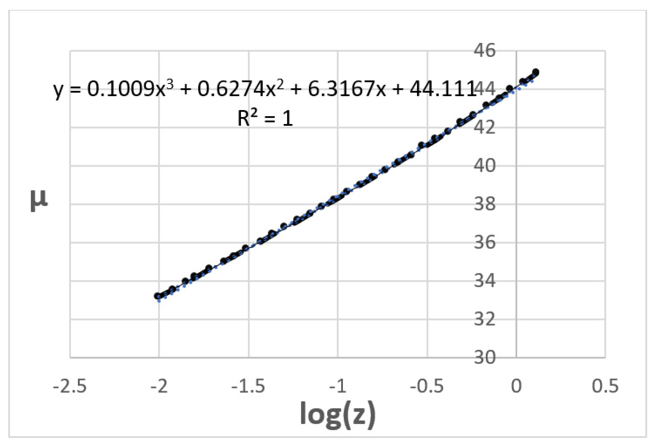
Figure 2.
ln(z+1)/t Hubble diagram for the 31 calculated z/d data points.
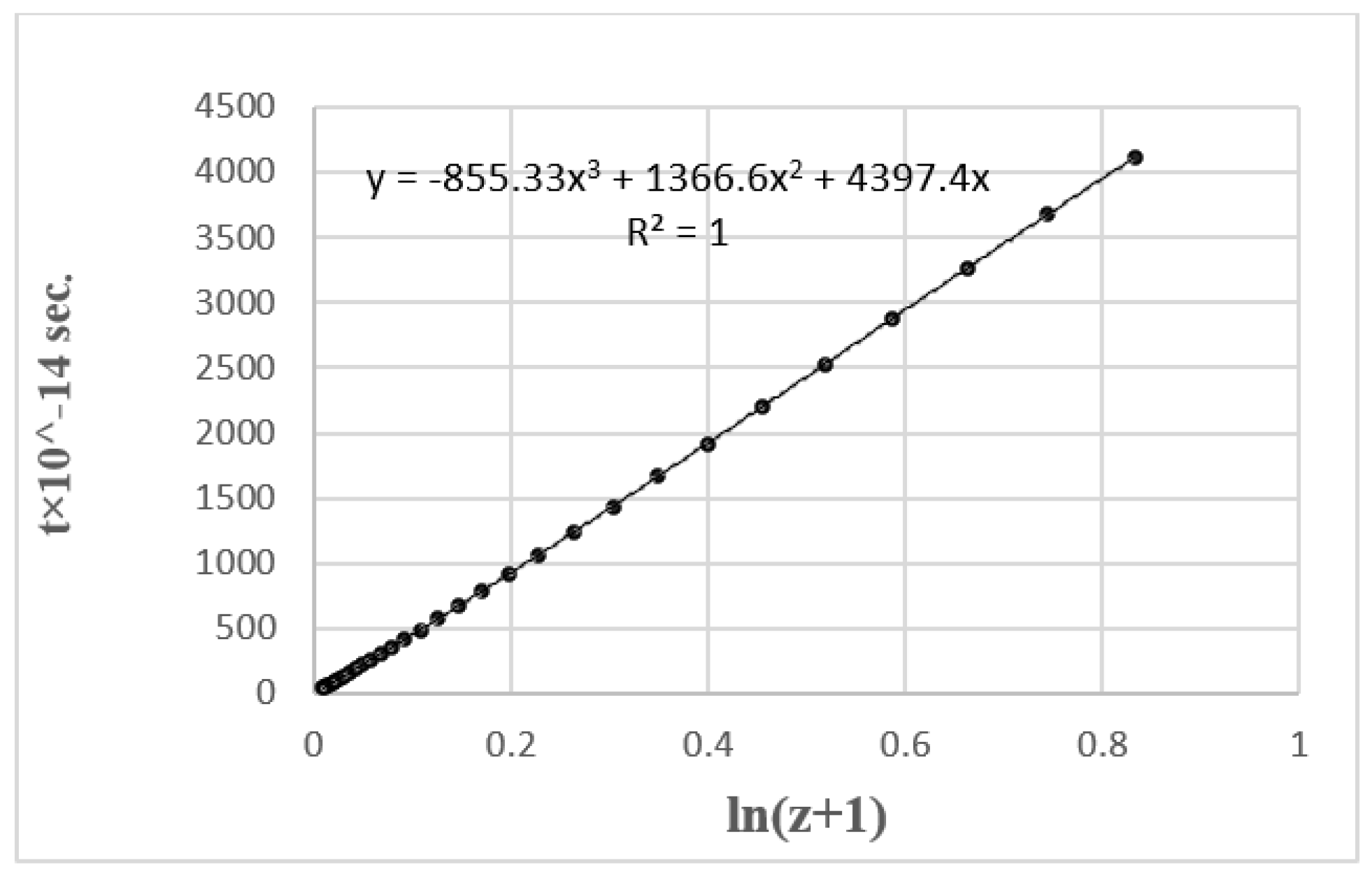
Figure 3.
Linear HDs for the calculated data (dots) and for the log(z)/µ (triangles) and d/ln(z+1) (squares) models.
Figure 3.
Linear HDs for the calculated data (dots) and for the log(z)/µ (triangles) and d/ln(z+1) (squares) models.
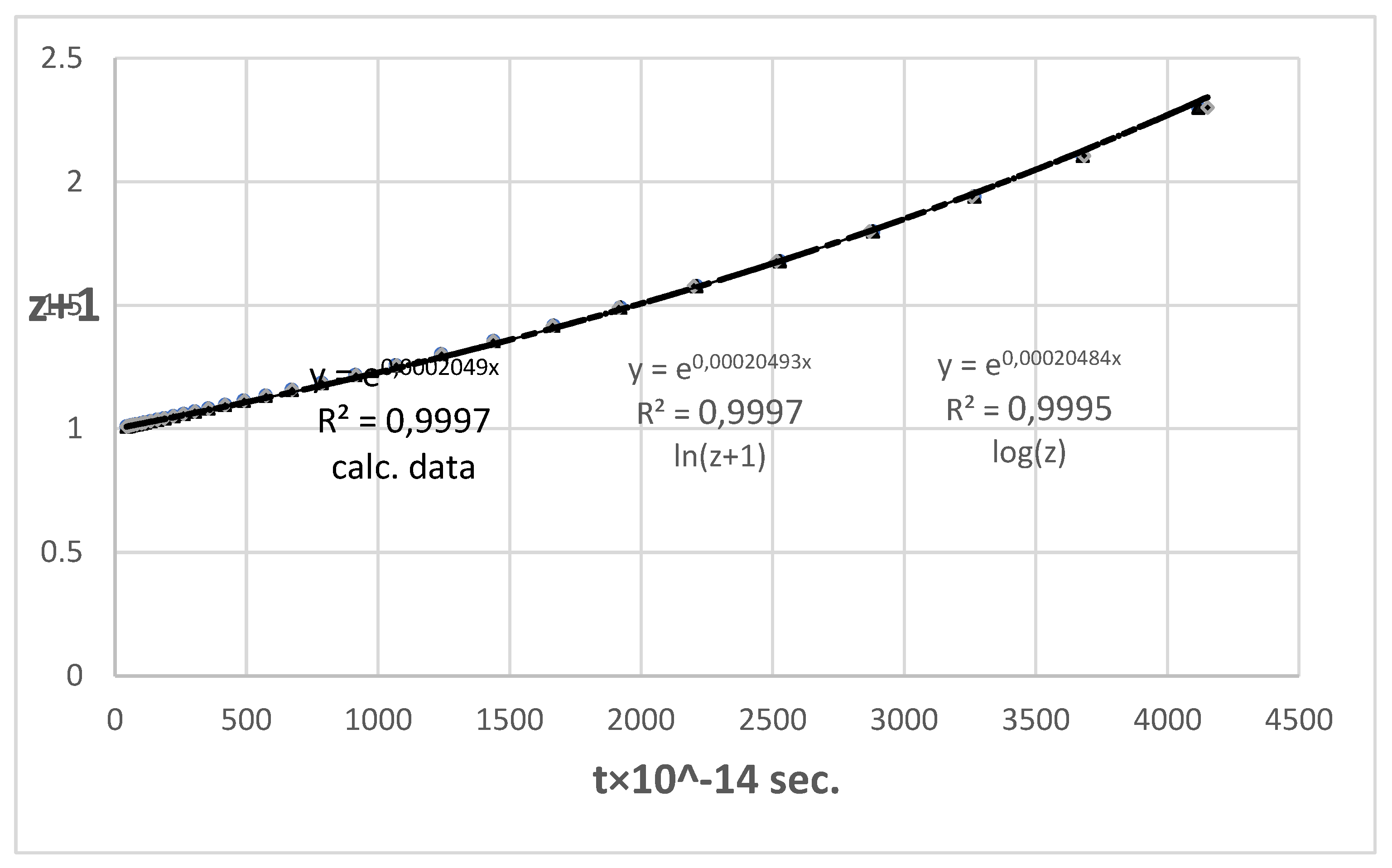
Figure 4.
Log(z)/µ Hubble diagram of the observed GRB data.
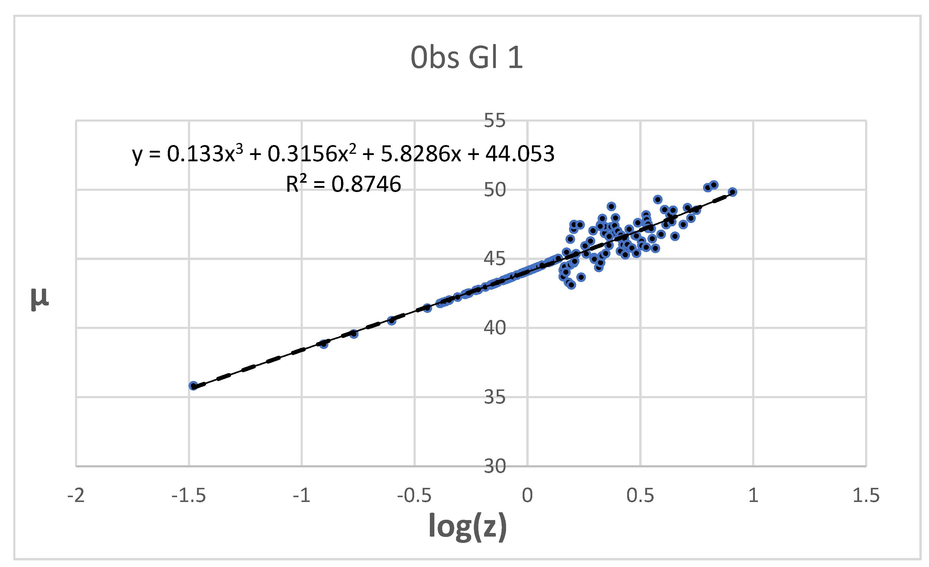
Figure 5.
hCDM = 0.7 (triangles), best fit of the observed data (squares), hTL = 0.66 (dots).
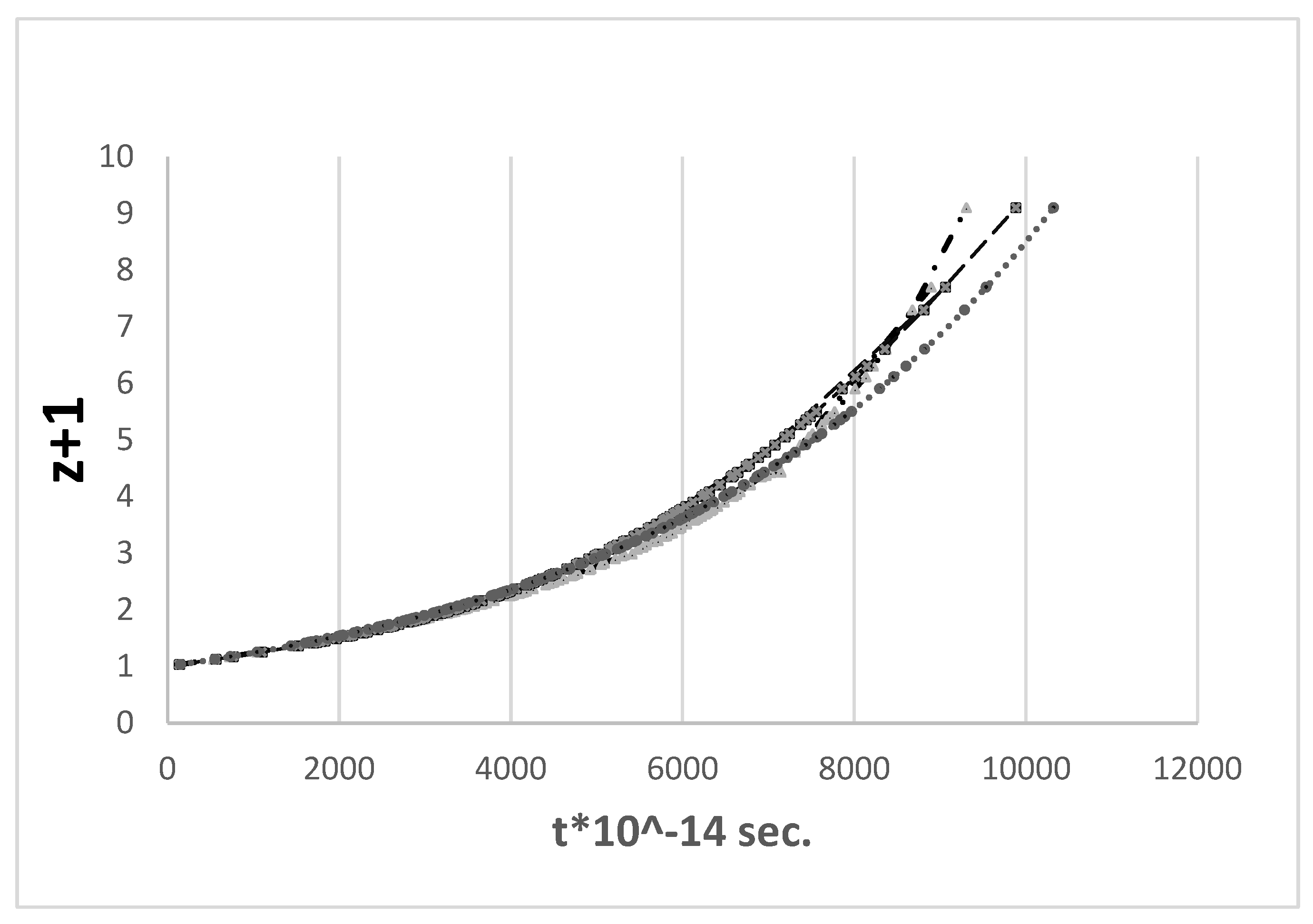
Figure 6.
Linear HD on the t/(z+1) scale of the observed GRB data,.
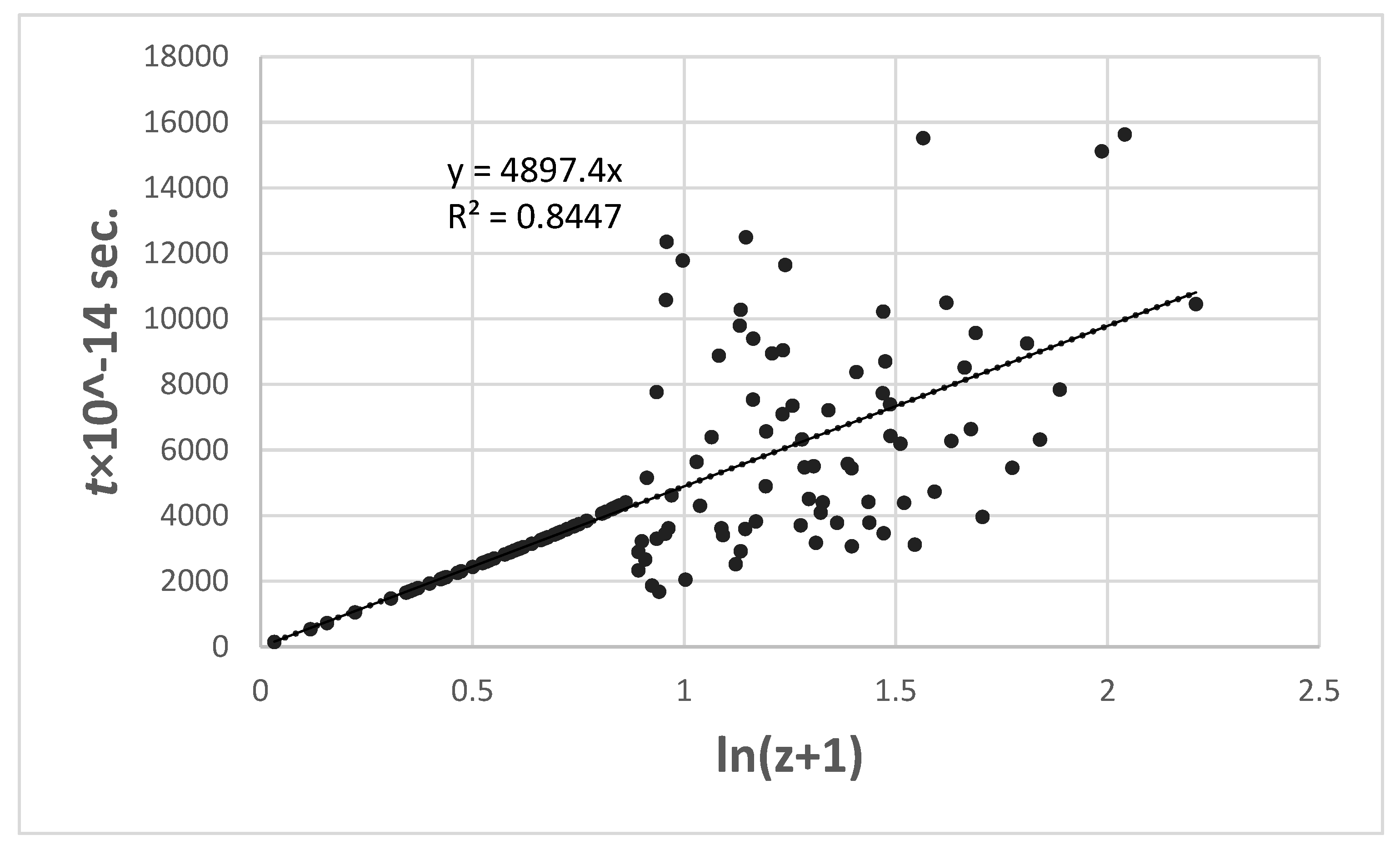
Figure 7.
t/ln(z+1) HD for the observed GRB data.
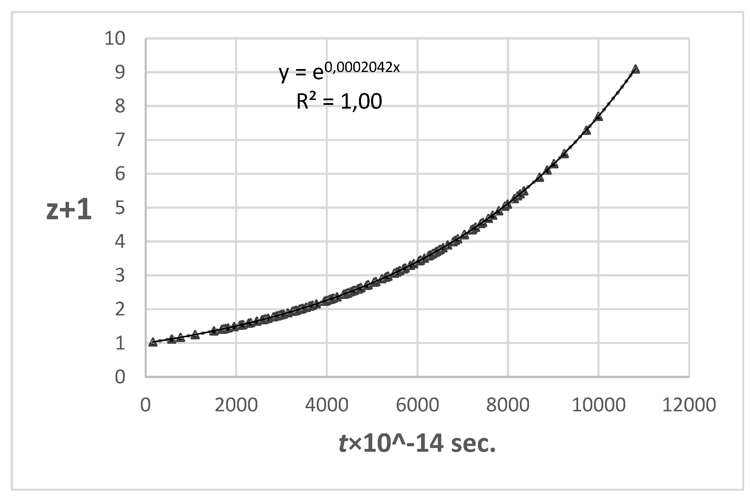

Table 1.
Descriptive statistics from the considered GRB data sets.
| Data set | (b) | (c) | (d) |
| No. of data points | 138 | 193 | 134 |
| z range | 0.031–8.1 | 0.03354–8.1 | 1.48–9.3 |
| Data points z ⸖ 5 | 6 | 5 | 5 |
| R2 | 0.8746 | 0.7848 | 0.8241 |
| ∑χ2(best fit:obs) | 1.9193 | 5.1282 | 2.8849 |
| ∑χ2/data point | 0.0139 | 0.02657 | 0.02153 |
| Standard deviation | 2.196 | 2.2256 | 2.2623 |
Table 2.
Fit parameters on the linear log(z)µ and ln(z+1)/t scales.
| Parameter 1 | Parameter2 | Parameter3 | Parameter 0 | |
|---|---|---|---|---|
| log fit | 0.1009 | 0.6274 | 6.3167 | 44.111 |
| ln fit | −855.33 | 1366.6 | 4397.4 | 0 |
Table 3.
Goodness of fit indicators the linear log(z)µ and ln(z+1)/t scales.
| Fit coordinates | ∑χ2µcalc: µ fit |
R2 | P test | Chiqu-test | F test |
|---|---|---|---|---|---|
| log(z)/µ | 2.673×10⁻⁵ | 1 | 0.9999985 | 1 | 0.9987774 |
| ln(z+1)/t | 1.810×10⁻⁶ | 1 | 1 | 1 | 0.9987774 |
Table 4.
Hubble constants and variances for the linear t/(z+1) HD.
| Model | Calculated data | ln fit | log fit |
|---|---|---|---|
| h | 0.6322 | 0.6322 | 0.6319 |
| R2 | 0.99967 | 0.99967 | 0.99948 |
Table 5.
Equivalent values for hCDM and hTL.
| hCDM | hTL | hTL/hCDM |
|---|---|---|
| 73 | 65.92 | 0.9031 |
| 70 | 63.22 | 0.9031 |
| 68 | 61.41 | 0.9031 |
Table 6.
Comparison of ∑ χ2 values for hCDM = 0.70, hTL = 0.70 and the Best fit hTL = 0 66 with the observed data in the RS range 0.031–8.1.
Table 6.
Comparison of ∑ χ2 values for hCDM = 0.70, hTL = 0.70 and the Best fit hTL = 0 66 with the observed data in the RS range 0.031–8.1.
| Model, calc. µ | hCDM = 0.70 | hTL = 0.66 | hTL = 0.70 |
|---|---|---|---|
| ∑ χ2 µobs/µcalc | 1.9415 | 1.9397 | 1.9923 |
Table 7.
Fit coefficients for the log(z)/µ Hubble diagram.
| Parameter 1 | Parameter 2 | Parameter 3 | Parameter 0 | R2 |
|---|---|---|---|---|
| 0.133 | 0.3156 | 5.8286 | 44.0533 | 0.8746 |
Disclaimer/Publisher’s Note: The statements, opinions and data contained in all publications are solely those of the individual author(s) and contributor(s) and not of MDPI and/or the editor(s). MDPI and/or the editor(s) disclaim responsibility for any injury to people or property resulting from any ideas, methods, instructions or products referred to in the content. |
© 2023 by the authors. Licensee MDPI, Basel, Switzerland. This article is an open access article distributed under the terms and conditions of the Creative Commons Attribution (CC BY) license (http://creativecommons.org/licenses/by/4.0/).
Copyright: This open access article is published under a Creative Commons CC BY 4.0 license, which permit the free download, distribution, and reuse, provided that the author and preprint are cited in any reuse.


