Predicting Operating Income via a Generalized Operating Leverage Model

Sherwood Lane Lambert; Kevin Krieger; Nathan Mauck

doi:10.20944/preprints202311.0806.v1

Submitted:

09 November 2023

Posted:

13 November 2023

You are already at the latest version

Abstract

We propose a generalized, practitioner-oriented operating leverage model for predicting operating income using Standard and Poor’s Compustat items: SALE (net sales), COGS (cost of sales), DP (total depreciation and amortization), XSGA (selling, general, and administrative expenses), and OIADP (operating income after depreciation and amortization). Prior research finds that OIADP = SALE - COGS - DP - XSGA; hence, our model includes all aggregate revenues and expenses comprising OIADP. Also, prior research finds COGS is “much less” sticky than DP and XSGA; hence, we use COGS as a proxy for total variable costs and DP and XSGA as proxies for sticky fixed costs. We introduce a new adjustment to the textbook operating leverage model so that SALE-to-COGS remains constant for the reference and forecast periods. Also, inspired by prior research, we introduce adjustments to DP and XSGA for cost stickiness. We find our generalized operating leverage model improves estimates of changes in next-quarter and next-year OIADP compared to textbook operating leverage predictions, which are special cases of our model.

Keywords:

Forecasting

;

accounting

;

earnings

Subject:

Business, Economics and Management - Accounting and Taxation

I. INTRODUCTION

We propose an earnings forecast model using the Standard and Poor’s (S&P) Compustat database items that Casey et al. (2016) show coincide with Compustat OIADP1. Specifically, we utilize SALE (net sales revenue), COGS (cost of goods sold), DP (total depreciation and amortization), XSGA (selling, general, and administrative expenses), and OIADP (operating income after depreciation and amortization). Casey et al. (2016) show that equation [1] generally holds in Compustat for each company for each year and quarter.

OIADP = SALE - COGS - DP - XSGA [1]

Anderson, Banker, and Janakiraman (2003) (hereafter, “ABJ”) find that XSGA is a mixture of fixed and variable costs that, on average, increases more for a 1% increase in SALE than it decreases for a 1% decrease in SALE, thereby exhibiting “sticky” cost behavior. Shust and Weiss (2014) show that depreciation is also a stick accrual accounting cost. Chen et al. (2019) find that COGS is mostly variable while DP, like XSGA, is also a sticky, mixed cost. Based on this prior research, we use the Compustat cost items in [1] as proxies for the variable and fixed costs in the traditional cost-volume-profit (CVP) income statement. We also apply such proxies in calculating operating leverage derived from the CVP income statement that managerial and cost accounting textbooks generally describe as:

Operating Leverage = Contribution Margin / Operating Income

where Contribution Margin = Total Sales Revenue - Total Variable Costs [2]

Using [2], our unadjusted proxy for Operating Leverage is2:

Operating Leverage = (SALE – COGS) / OIADP [3]

Managerial accounting textbooks usually state the assumptions that must be true for operating leverage derived from CVP to predict future operating income. For example, Hilton (2023) says that, within the relevant range, total fixed expenses must remain constant as activity changes, and the unit variable expense remains unchanged as activity varies. We provide mathematical proof in Appendix A that (1) the ratio of total sales-to-total variable costs, and (2) total fixed costs must each remain constant in the current (reference) and forecast periods for the traditional operating leverage (see above), multiplied by the future period’s percent change in sales, to accurately predict a future period's operating income.

In reality, SALE-to-COGS will generally vary as companies change the product mix, selling prices, and sales markups, and as the costs of goods and services vary. Hence, we introduce an adjustment so that SALE-to-COGS remains constant by estimating each company’s future period’s ratio of SALE-to-COGS and using this estimate to modify operating leverage model [3] so that the current and future periods' SALE-to-COGS ratios are equal. Additionally, prior research has demonstrated that XSGA and DP are asymmetrically variable (sticky) with increases and decreases in sales (ABJ; Shust and Weiss, 2014). Thus, we follow ABJ and Shust and Weiss (2014) by adjusting XSGA and DP in model [3] so that, on average, these costs change in a (more realistic) sticky manner as SALE changes. These modifications result in a generalized model of operating leverage for which textbook operating leverage is a special case with invariant sales-to-total-variable costs and fixed costs.

We assess our modified operating leverage model's predictive power by regressing the change in OIADP, sized by total assets, on the change in our model’s estimate of OIADP, sized by total assets. We also study the error levels of our model's estimates. We evaluate our model for predicting firms’ OIADP in the next quarter and next year.

To our knowledge, we are the first to develop an operating leverage model from the perspective of equation [1] identified by Casey et al. (2016). Additionally, our paper is the first, to our knowledge, to develop a procedure for adjusting an operating leverage proxy to incorporate the constant sales-to-total-variable-costs (SALE-to-COGS) assumption. Also, inspired by prior research findings, we adjust DP and XSGA in our model for cost stickiness. We evaluate our Compustat-based operating leverage model’s ability to predict firms’ next-quarter and next-year OIADP via regression analyses and by assessing the prediction errors. Our operating leverage model improves the forecast accuracy of next-quarter and next-year OIADP compared to earlier models, which do not adjust for constant sales-to-total-variable costs or sticky depreciation, amortization, and SG&A costs. Financial analysts, investors, and other practitioners who use S&P’s Compustat data may benefit by using our operating leverage model when forecasting companies’ next-quarter and next-year operating incomes.

The paper proceeds with a discussion of prior research on the behavior of accounting costs. Next, we discuss in more detail the methodology outlined in the Introduction and then present our detailed findings. We then summarize our findings, discuss future research, and conclude.

II. BACKGROUND

Usually, a firm’s operating leverage is not explicitly known to external users because generally accepted accounting principles (GAAP) do not require corporations to specify costs as variable or fixed. As a result, users of general-purpose financial statements must estimate corporations’ variable and fixed costs and, hence, operating leverages. For example, Lev (1974, p. 633) used time-series linear regressions to estimate the beta average variable costs for each studied firm and found a positive relationship between estimated variable and fixed costs (traditional operating leverage) and returns. Prior to ABJ, it was commonly accepted that Selling and Administrative (S&A) were approximately fixed costs: “Most administrative costs are approximately fixed, therefore, a disproportionate (to sales) increase is considered a negative signal suggesting, among other things, a loss of managerial cost control or an unusual sales effort (Bernstine [1988, p. 692])” (Lev and Thiagarajan, 1993, p. 196). However, ABJ found that selling, general, and administrative (SG&A) costs behave with “sticky” variability partly because managers make decisions that change the resources committed to activities.

Lipe (1986) showed that six GAAP financial statement components (gross profits, general and administrative expense, depreciation expense, interest expense, income taxes, and other items) provide information incremental to earnings for predicting future earnings and returns. Lev and Thiagarajan (1993) identified fundamental signals in GAAP financial statements that security analysts claimed were useful in evaluating corporations’ future earnings and returns. The authors found that these fundamentals added approximately 70%, on average, to the explanatory power of earnings alone with respect to excess returns. Abarbanell and Bushee (1997) found that the fundamental signals identified by Lev and Thiagarajan (1993) were also relevant to predicting future earnings. Ciftci et al. (2016) demonstrated that considering the variability and stickiness of costs improves analysts’ earnings forecasts, especially when sales decline.

Fairfield et al. (1996) use line items from GAAP income statements to classify earnings into operating and non-operating income components to forecast future Return on Equity (ROE). The study found incremental predictive content for the average firm from disaggregating earnings into operating income separate from non-operating income, income taxes, special items, extraordinary items, and discontinued operations. Further disaggregation did not improve forecasts for one-year-ahead ROE. The studies’ operating income variable (OPINC) includes five explanatory variables from GAAP income statements: gross margin, selling, general and administrative expenses, depreciation expense, interest expense, and minority income. The study found that these five components of operating income are reasonably homogeneous with respect to providing information about future profitability. In contrast, the evidence indicated that the information content of non-operating income, income taxes, extraordinary items, and discontinued operations may be relevant to outcomes other than future profitability. Additionally, the OPINC model has similar accuracy when predicting ROE or operating income. In a comparable study, Sloan (1996) uses line items contained in GAAP financial statements to predict future ROE based on past cash flows and accruals components of earnings.

Banker and Chen (2006) propose an earnings forecast model that decomposes earnings into components that reflect the variability of costs with sales revenue and sticky costs that respond differently to sales increases and decreases. The authors’ model forecasts earnings more accurately than the Fairfield et al. (1996) model based on items in operating income or the Sloan (1996) model, which disaggregates earnings into cash flows and accruals components. However, all three models are less accurate than analysts’ consensus forecasts that consider other factors, such as the macroeconomy and industry contexts. Our generalized operating leverage model differs from the Banker and Chen (2006) approach by:

Using the Casey et al. (2016) identity that Compustat SALE - COGS - DP - XSGA equates to Compustat OIADP
Predicting OIADP operating income as opposed to Return on Equity (ROE)
Specifying Compustat depreciation and amortization (DP) and selling, general, and administrative costs (XSGA) as sticky costs following Shust and Weiss (2014) and Chen et al. (2019)
Employing COGS as a proxy for total variable costs following Chen et al. (2019)
Predicting future COGS by using estimated future SALE-to-COGS ratio

Our generalized operating leverage model provides practitioners with a parsimonious earnings forecast model that directly estimates next-quarter and next-year operating income (OIADP) using only the Compustat items SALE, COGS, DP, and XSGA.

Other research has shown that losses have a lower earnings response coefficient (ERC) than the profits liquidation option (Hayn, 1995).

Banker and Byzalov (2014) review the theory of cost behavior and problems with estimating traditional variable and fixed costs, demonstrating that costs have asymmetric behavior that can be “sticky” and “anti-sticky” and that traditional “fixed” and “variable” cost classifications are extreme cases. Ciftci and Zoubi (2019) find more stickiness for small current sales changes than for large current sales changes.

Other research has examined traditional operating leverage versus financial leverage (Mandelker and Rhee 1984; Simintzi et al. 2015). Furthermore, studies in finance have used traditional operating leverage to study stock return properties (Sagi and Seasholes 2007; Gulen et al. 2011; Novy-Marx 2011; Donangelo 2014; Banker et al. 2018) and cost of equity (e.g., Chen et al. 2011). Mandelker and Rhee (1984) study the joint impact of operating leverage and financial leverage on systematic risk and find a significant correlation between the two types of leverage. Simintzi et al. (2015) find that employment protection increases operating leverage and reduces financial leverage. Novy-Marx (2011) measures operating leverage as cost of goods sold plus selling, general, and administrative expenses, divided by total assets, and shows that companies with higher operating leverage have higher expected returns. Donangelo (2014) shows that firms face greater operating leverage by providing flexibility to mobile workers. Rouxelin et al. (2018) find that changes in aggregate cost stickiness help predict future macroeconomic outcomes, such as the unemployment rate, and thereby provide relevant information for macroeconomic policy.

III. METHODOLOGY

Data

Our data source is S&P’s Compustat database for North American Companies. For quarterly data, we study fiscal year 2005 quarter 2 through fiscal year 2021 quarter 4. For annual data, we analyze fiscal years 1984 through 2021.

Methodology for Predicting Quarterly OIADP

We introduce a modified operating leverage model that seeks to account for the variability in the SALE-to-COGS ratio and the stickiness of XSGA and DP. Our adjusted operating leverage model is parsimonious, yet it considers all the aggregated Compustat items that articulate with OIADP, namely all the accrual accounting revenues and expenses from continuing operations summarized in SALE, COGS, XSGA, and DP. We begin with our base operating leverage model using the Compustat income statement items that articulate with operating income. Next, we create the intermediate model by modifying the base model to account for changes in the SALE-to-COGS ratio during the forecast period. Finally, we develop the generalized model from the intermediate model by accounting for the stickiness of XSGA and DP.

Chen et al. (2019) show that COGS is much less sticky than XSGA and DP. Hence, we treat COGS as a proxy for total variable cost in our CVP and operating leverage models. Bostwick et al. (2016) found that S&P subtracts DP from cogs to derive COGS when companies’ financial statements do not quantify the allocated depreciation and amortization amounts.3 A manufacturing company’s deprecation costs may be substantial, such as plant and equipment depreciation.

In Appendix B, we use our quarterly data and ABJ methodology to compute 0.484 (0.205) as the factor by which DP increases (decreases), on average, for a 1% increase (1% decrease) in SALE. Similarly, we compute 0.377 (0.235) as the factor by which XSGA increases (decreases), on average, for a 1% increase (1% decrease) in SALE. These quarterly results using our data corroborate ABJ and Shust and Weiss (2014) finding that XSGA and DP are sticky costs. We use these four factors to adjust for the stickiness of DP and XSGA in our generalized model [11] for predicting next-quarter OIADP. Also, we find quarterly COGS increasing 0.879 (decreasing 0.717) for a 1% increase (1% decrease) in SALE. These results corroborate Chen et al. (2019) and further support our use of COGS as a proxy for total variable costs in our Compustat proxy for CVP in Figure 1.

Restating Operating Leverage For Constant SALE / COGS Ratio For Quarters

When estimating next-quarter OIADP_t+1 during quarter t, we adjust for the seasonality of quarterly accounting data (Chang et al. 2017, Welch 1984, Griffin 1977, Jones and Litzenberger 1969). Hence, we use quarter t-3 Compustat data when forecasting OIADP for t+1. We use the Compustat variables in [1] to create the CVP income statement proxy shown in Figure 1.

Managerial accounting textbooks define a company’s operating leverage for a period as operating income/contribution margin. Using Figure 1’s Compustat version of the CVP income statement, company i’s operating leverage (OL) for quarter t-3 is:

BASE_QTR_OL_i,t-3 = (SALE_i,t-3 - COGS_i,t-3) / OIADP_i,t-3 [4]

Managerial accounting textbooks often show for company i, current period t, and future period t+n, that:

Future operating income_i,t+n = (1 + operating income_i,t) *

(operating leverage_i,t * percent change in sales from period t to period t+n) [5]

With our base model, we assume that the ratio of SALE-to-COGS remains constant and the total DP and XSGA costs remain fixed for quarters t-3 and t + 1. Then, our base quarterly model is as follows:

BASE_MODEL_EST_QTR_OIADP_i,t+1 =

(1 + (CHG_QTR_SALE_i,t+1 * BASE_QTR_OL_i,t-3)) * OIADP_i,t-3

where:

CHG_QTR_SALE_i,t+1 =

(((average of SALE for periods t-2 through t) - SALE_i,t-3) / SALE_i,t-3) [6]

However, SALE/COGS can vary from period to period, such as when firms change sales markups. Therefore, we develop model [7] where we estimate SALE_i,t+1/COGS_i,t+1 based on prior periods’ SALE/COGS history and adjust COGS_i,t-3 so that SALE_i,t-3/adjusted COGS_i,t-3 equals estimated SALE_i,t+1/COGS_i,t+1.

EST_QTR_SALE_to_COGS_i,t+1 =

(1 + (((average of SALE-to-COGS for periods t-2 through t) - SALE_to_COGS_i,t-3) / SALE_to_COGS_i,t-3)) * SALE_to_COGS_i,t-3 [7]

We then compute restated operating leverage for the reference (t-3) quarter as:

RESTATED_QTR_OL_i,t-3 =

(SALE_i,t-3 - (SALE_i,t-3 / EST_QTR_SALE_to_COGS_i,t+1)) / (SALE_i,t-3 - (SALE_i,t-3 / (EST_QTR_SALE_to_COGS_i,t+1 / COGS_i,t+1)) - DP_i,t-3 - XSGA_i,t-3) [8]

This intermediate model utilizes RESTATED_QTR_OL_i,t-3, assumes DP and XSGA are fixed costs, and does not adjust for sticky DP or XSGA when estimating next-quarter OIADP_i,t+1 thusly:

INTERMEDIATE_MODEL_ESTIMATED_QTR_OIADP_i,t+1 =

(1 + (CHG_QTR_SALE_i,t+1 * RESTATED_QTR_OL_i,t-3)) *

(SALE_i,t-3 - (SALE_i,t-3 / EST_QTR_SALE_to_COGS_i,t+1) - DP_i,t-3 - XSGA_i,t-3) [9]

In the generalized quarterly model, we modify [8] and [9] to adjust for sticky DP and XSGA using the factors in Table 1B and compute RESTATED_QTR_OL_WITH_STICKY_DP_AND_XSGA_i,t-3 as follows:

If CHG_QTR_SALE_i,t+1 ≥ 0

RESTATED_QTR_OL_WITH_STICKY_DP_AND_XSGA_i,t-3 =

(SALE_i,t-3 - SALE_i,t-3 / EST_QTR_SALE_to_COGS_i,t+1) /

(SALE_i,t-3 - SALE_i,t-3 / EST_QTR_SALE_to_COGS_i,t+1 - DP_i,t-3 – XSGA_i,t-3 -

(CHG_QTR_SALE_i,t+1 * 0.484 * DP_i,t-3) - (CHG_QTR_SALE_i,t+1 * 0.377 * XSGA_i,t-3))

If CHG_QTR_SALE_i,t-1 < 0

RESTATED_QTR_ OL_WITH_STICKY_DP_AND_XSGA_i,t-3 =

(SALE_i,t-3 – SALE_i,t-3 / EST_QTR_SALE_to_COGS_i,t+1) /

(SALE_i,t-3 – SALE_i,t-3 / EST_QTR_SALE_to_COGS_i,t+1 - DP_i,t-3 – XSGA_i,t-3 -

(CHG_QTR_SALE_i,t+1 * 0.205 * DP_i,t-3) - (CHG_QTR_SALE_i,t+1 * 0.235 * XSGA_i,t-3)) [10]

Then, we estimate next quarter’s OIADP_i,t+1 using our generalized (full) model thusly:

If CHG_QTR_SALE_i,t+1 ≥ 0

FULL_MODEL_ESTIMATED_QTR_OIADP_i,t+1 = (1 + (CHG_QTR_SALE_i,t+1 *

RESTATED_QTR_OL_WITH_STICKY_DP_AND_XSGA_i,t-3)) *

(SALE_i,t-3 - (SALE_i,t-3 / EST_QTR_SALE_to_COGS_i,t+1) - DP_i,t-3 - XSGA_i,t-3 -

(CHG_QTR_SALE_i,t+1 * 0.484 * DP_i,t-3) - (CHG_QTR_SALE_i,t+1 * 0.377 * XSGA_i,t-3))

If CHG_QTR_SALE_i,t+1 < 0

FULL_MODEL_ESTIMATED_QTR_OIADP_i,t+1 = (1 + (CHG_QTR_SALE_i,t+1 *

RESTATED_QTR _OL_WITH_STICKY_DP_AND_XSGA_i,t-3)) *

(SALE_i,t-3 - (SALE_i,t-3 / EST_QTR_SALE_to_COGS_i,t+1) - DP_i,t-3 - XSGA_i,t-3 -

(CHG_QTR_SALE_i,t+1 * 0.205 * DP_i,t-3) - (CHG_SALE_i,t+1 * 0.235 * XSGA_i,t-3))

where:

EST_QTR_SALE_to_COGS_i,t+1 =

(1 + (((average of SALE-to-COGS for quarters t-2 through t) -

[SALE_i,t-3 / COGS_i,t-3]) / [SALE_i,t-3/ COGS_i,t-3])) * [SALE_i,t-3 / COGS_i,t-3] [11]

Using linear regression analysis, we regress CHG_QTR_OIADP_i,t+1 on

CHG_QTR_EST_OIADP_i,t+1 sized by total assets (AT_i,t-1)

where:

CHG_QTR_OIADP_i,t+1 = (OIADP_i,t+1 - OIADP_i,t-3) / AT_i,t-1 [12]

and

CHG_QTR_EST_OIADP_i,t+1 =

(ESTIMATED_QTR_OIADP_i,t+1 - OIADP_i,t-1) / AT_i,t-1 [13]

In addition, we consider the distribution of the absolute value of the error percent for our model estimates of quarterly OIADP_i,t+1 as:

Absolute Value of Estimate Error =

Absolute Value ((OIADP_i,t+1 - ESTIMATED_QTR_OIADP_i,t+1) / OIADP_i,t+1) [14]

Methodology for Predicting Annual OIADP

Our models for predicting next-year OIADP mirror our models for predicting next-quarter OIADP, except t denotes the fiscal year, and the reference year is the current year, t, rather than the third prior quarter. Hence, the base (textbook) operating leverage model [3] for predicting next-year OIADP is:

BASE_1YR_OL_i,t = (SALE_i,t - COGS_i,t) / OIADP_i,t [15]

With our base model, we assume that the ratio of SALE-to-COGS remains constant, and the total DP and XSGA costs remain fixed for years t and t + 1. Hence, our base (textbook) model for predicting next-year OIADP is:

BASE_MODEL_EST_1YR_OIADP_i,t+1 =

(1 + (CHG_1YR_SALE_i,t+1 * BASE_1YR_OL_i,t)) * OIADP_i,t

where

CHG_1YR_SALE_i,t+1 =

(SALE_i,t - ((SALE_i,t + SALE_i,t-1) / 2)) / ((SALE_i,t + SALE_i,t-1) / 2) [16]

Using annual data and making only our adjustment that enables constant SALE-to-COGS, restated operating leverage is:

RESTATED_1YR_OL_i,t =

(SALE_i,t - (SALE_i,t / EST_1YR_SALE_to_COGS_i,t+1)) /

(SALE_i,t - (SALE_i,t / EST_1YR_SALE_to_COGS_i,t+1) - DP_i,t - XSGA_i,t)

where EST_1YR_SALE_to_COGS_i,t+1 =

((SALE_i,t / COGS_i,t) + (SALE_i,t-1 / COGS_i,t-1)) / 2 [17]

Assuming that DP and XSGA are fixed and, hence, do not require adjusting for sticky cost behavior, our intermediate model for estimating next-year OIADP_i,t+1 becomes:

INTERMEDIATE_MODEL_ESTIMATED_1YR_OIADP_i,t+1 =

(1 + (CHG_1YR_SALE_i,t+1 * RESTATED_1YR_OL_i,t)) *

(SALE_i,t - (SALE_i,t / EST_1YR_SALE_to_COGS_i,t+1) - DP_i,t - XSGA_i,t) [18]

In Appendix C, we use our yearly data and ABJ methodology to compute 0.647 (0.393) as the factor by which DP increases (decreases), on average, for each 1% increase (1% decrease) in SALE. Similarly, we compute 0.440 (0.309) as the factor by which XSGA increases (decreases), on average, for a 1% increase (1% decrease) in SALE. We use these four factors to adjust for the stickiness of DP and XSGA in our generalized models [19] and [20] for predicting next-year OIADP. These results using our annual data are in line with ABJ and Shust and Weiss (2014) that XSGA and DP are sticky costs. Also, Appendix C results show COGS increases 0.880 (decreases 0.834) for a 1% increase (1% decrease) in annual SALE with adjusted R-square equal to 0.589. These results confirm Chen et al.’s (2019) findings that COGS is mostly variable and provide additional support for using COGS as a proxy for total variable costs in our Compustat proxy for CVP in Figure 1.

If we then adjust DP and XSGA as sticky costs following the prior research previously discussed, we compute RESTATED_1YR_OL_WITH_STICKY_DP_AND_XSGA_i,t as follows:

If CHG_1YR_SALE_i,t+1 ≥ 0

RESTATED_1YR_OL_WITH_STICKY_DP_AND_XSGA_i,t =

(SALE_i,t - SALE_i,t / EST_1YR_SALE_to_COGS_i,t+1) /

(SALE_i,t - SALE_i,t / EST_1YR_SALE_to_COGS_i,t+1 - DP_i,t - XSGA_i,t -

(CHG_1YR_SALE * 0.647 * DP_i,t) - (CHG_1YR_SALE * 0.440 * XSGA_i,t))

If CHG_1YR_SALE_i,t+1 < 0

RESTATED_1YR_OL_WITH_STICKY_DP_AND_XSGA_i,t =

(SALE_i,t - SALE_i,t / EST_1YR_SALE_to_COGS_i,t+1) /

(SALE_i,t - SALE_i,t / EST_1YR_SALE_to_COGS_i,t+1 - DP_i,t - XSGA_i,t -

(CHG_1YR_SALE * 0.393 * DP_i,t) - (CHG_1YR_SALE * 0.309 * XSGA_i,t)) [19]

Then, we estimate the next fiscal year’s OIADP_t+1 using our generalized (full) model thusly:

If CHG_1YR_SALE_i,t+1 ≥ 0

ESTIMATED_1YR_OIADP_i,t+1 =

(1 + (CHG_1YR_SALE * RESTATED_1YR_OL_WITH_STICKY_DP_AND_XSGA_i,t)) *

(SALE_i,t - (SALE_i,t / EST_1YR_SALE_to_COGS_i,t+1) - DP_i,t - XSGA_i,t -

(CHG_1YR_SALE * 0.647* DP_i,t) - (CHG_1YR_SALE * 0.440 * XSGA_i,t))

If CHG_1YR_SALE_i,t+1 < 0

ESTIMATED_1YR_OIADP_i,t+1 =

(1 + (CHG_1YR_SALE * RESTATED_1YR_OL_WITH_STICKY_DP_AND_XSGA_i,t)) *

(SALE_i,t - (SALE_i,t / EST_1YR_SALE_to_COGS_i,t+1) - DP_i,t - XSGA_i,t -

(CHG_1YR_SALE_i,t+1 * 0.393 * DP_i,t) - (CHG_1YR_SALE_i,t+1 * 0.309 * XSGA_i,t)) [20]

We regress annual CHG_1YR_OIADP_i,t+1 on CHG_1YR_EST_OIADP_i,t+1 sized by AT_i,t-1 where:

CHG_1YR_OIADP_i,t+1 = (OIADP_i,t+1 - OIADP_i,t) / AT_i,t-1 [21] CHG_1YR_EST_OIADP_i,t+1 = (ESTIMATED_1YR_OIADP_i,t+1 - OIADP_i,t) / AT_i,t-1 [22]

Also, we analyze the strata and percentiles of the absolute values of the errors for our generalized, full model estimates of annual OIADP_i,t+1 as:

Absolute Value ((OIADP_i,t+1 - ESTIMATED_OIADP_t+1) / OIADP_i,t+1) [23]

Testing the Veracity of the Generalized Operating Leverage Model

Given [1], perfect knowledge of future SALE_i,t+1, COGS_i,t+1. DP_i,t+1, and` XSGA_i,t+1 should provide a perfect estimate of OIADP_i,t+1. Using this same perfect knowledge, the generalized (full) models [19] and [20] for predicting next-year OIADP become:

RESTATED_OL =

(SALE_i,t - (SALE_i,t / (SALE_i,t+1 / COGS_i,t+1))) /

(SALE_i,t - (SALE_i,t /(SALE_i,t+1 / COGS_i,t+1)) - DP_i,t+1 - XSGA_i,t+1) [24]

NEXT_YR_OPERATING_INCOME_i,t+1 =

(1 + (((SALE_i,t+1 - SALE_i,t) / SALE_i,t) * RESTATED_OL)) *

(SALE_i,t - (SALE_i,t / (SALE_i,t+1 / COGS_i,t+1)) - DP_i,t+1 - XSGA_i,t+1) [25]

Using NEXT_YR_OPERATING_INCOME_i,t+1 from [25] in [22], we obtain:

CHG_1YR_EST_OIADP_i,t+1 =

(NEXT_YR_OPERATING_INCOME_i,t+1 - OIADP_i,t) / AT_i,t-1

Regressing [21] on [22] produces linear regression results with Adj. R-square = 1.000, a standard error of the estimate = .00003584172, and beta = 1.000 (t-value = 81965653). Also, using model [23], the Absolute Value ((OIADP_i,t+1 - NEXT_YR_OPERATING_INCOME_i,t+1) / OIADP_i,t+1) = .00000000 for all but 87 of the 189,319 company-years tested for fiscal years 2005 through 20214. We obtain similar, untabulated results when testing our generalized (full) models [10] and [11] using our quarter data. These results are consistent with the accuracy of our generalized models’ forecasts of OIADP_i,t+1 depending entirely on the accuracy of forecasting SALE_i,t+1, the SALE_i,t+1 / COGS_i,t+1 ratio, and the stickiness of DP_t+1, and XSGA_t+1.

Consideration of Dow Jones Industrial Average (DJIA) Firms

We consider separately the results for DJIA firms because the 30 DJIA firms are “blue chip” stock companies that are well-established, financially sound, and sell generally high-quality, widely accepted products and services (Chen, 2023). We expect that our models will have higher explanatory power (adjusted R-square) and lower error rates in predicting OIADP for the DJIA corporations compared to all our studied companies.

IV. RESULTS AND DISCUSSION

Results for Estimating Quarterly OIADP

Table 1 shows the results from using the generalized (full) model [11] with operating leverage restated for constant SALE-to-COGS ratios and Appendix B factors used for adjusting sticky XSGA and DP to predict next-quarter OIADP_i,t+1. Analyses include results from regressing CHG_QTR_OIADP_i,t+1 [12] on CHG_QTR_EST_OIADP_i,t+1 [13] and distribution information for the absolute value of errors estimating next-quarter OIADP_i,t+1 [14]. Table 1 regression results show our generalized operating leverage model [11] positively and significantly predicts change in next-quarter OIADP for the 241,106 firm-quarters studied with a coefficient of 0.523 (t-value 169.009) and a 0.106 adjusted R-square. The median absolute value estimate error was 35.61%.

Table 1. Predicting Next Quarter Operating Income (OIADP) Using the Full Model [11]. All Companies for Fiscal Quarters t from 2005 Quarter 2 through 2021 Quarter 4.

Strata of Abs ERRORS	Count of Company-Years	Percent of Total Company-Years	Cumulative Percent of Company-Years	Percentiles of Company Years	Ordered Obs.	Percentile Abs ERROR
0% to 5%	25,531	10.59%	10.59%	1st Percentile:	2,411	0.46%
5% and 10%	23,020	9.55%	20.14%	5th Percentile:	12,055	2.29%
10% and 15%	19,239	7.98%	28.12%	10th Percentile:	24,111	4.71%
15% and 20%	15,962	6.62%	34.74%	25th Percentile:	60,276	12.97%
20% and 25%	13,663	5.67%	40.40%	Median:	120,553	35.61%
25% and 50%	45,670	18.94%	59.35%	75th Percentile:	180,829	93.24%
50% and 100%	41,436	17.19%	76.53%	90th Percentile:	216,995	245.35%
> 100%	56,585	23.47%	100.00%	95th Percentile:	229,050	499.47%
Total:	241,106	100.00%	100.00%	99th Percentile:	238,694	2498.45%
Linear Regression Results
N		Adj R-square		Coeff	t-value	p-value
241,105		0.106		0.523	169.009	0.000

Table 2 provides information about the relative predictive powers of the base, intermediate, and full models when estimating next-quarter OIADP. We used the same 241,106 company years in our analyses of the three models. Regression analysis for the base model [6] without restating operating leverage or adjusting DP or XSGA for sticky costs indicated a 0.121 coefficient (t-value 61.415) with explanatory, predictive power (adjusted R-square) of 0.015. The base model had a 40.40% median absolute value error. Using the intermediate model [9] that restates operating leverage to achieve constant SALE-to-COGS but does not adjust for the stickiness of DP or XSGA improves the adjusted R-square to 0.099 with a coefficient of 0.378 (t-value 162.314) and reduces the median absolute value error to 38.70%. Finally, results for the generalized (full) model [11] show that adding adjustments for DP and XSGA cost stickiness to the intermediate model improves the adjusted R-square to 0.106 with a coefficient of 0.523 (t-value 169.009) and reduces the median absolute value error to 35.61%.

Hayn (1995) found that the information content of losses affects the earnings relevance of accounting information. Table 3 summarizes the results from performing the same analyses on the data used in Table 1, except we select only those firm-quarters where current-quarter operating income (OIADP_i,t) and third-quarter prior operating income (OIADP_i,t-3) are positive. The regression estimation for positive operating income firm-quarters reported in Table 3 has a 0.147 adjusted R-square and 23.28% median absolute value error compared to the 0.106 adjusted R-square and 35.61% median absolute value error recorded in Table 1 for all firm-quarters studied.

Table 4 displays the results from using the generalized operating leverage model [11] to predict next-quarter operating income for only the DJIA companies. We use the same average factors specified in Table 1B for adjusting for sticky DP and XSGA and the same Compustat data analyzed for Table 1 except only for the DJIA members. The predictive power of our full model [11] in predicting quarterly OIADP for just the 30 DJIA companies increased to 0.338 adjusted R-square, with the median absolute value error reduced to 13.84%, as shown in Table 4. These results are consistent with our expectation that our model [11], which relies entirely on extrapolations using current and prior Compustat data, performs better when used to estimate next-quarter OIADP for more stable companies such as the DJIA companies.

Results for Estimating Annual OIADP

Table 5 shows the results of using the generalized (full) operating leverage model [19] and model [20] adjusted to predict next-year OIADP_i,t+1 with annual restated operating leverage and Appendix C factors for annual sticky DP and XSGA. Analyses include results from regressing CHG_1YR_OIADP_i,t+1 [21] on CHG_1YR_EST_OIADP_i,t+1 [22] for annual data and distribution details for the absolute value errors estimating next-year OIADP [23]. Table 5’s results show our generalized (full) models [19] and [20] predicted next-year OIADP for the 188,777 company-years studied with a coefficient of 0.259 (t-value 113.678), a 0.064 adjusted R-square, and 36.15% median accuracy.

Table 6 displays the results from predicting next-year operating income (OIADP_i,t+1) using the same generalized (full) operating leverage models [19] and [20] as seen in Table 5 but for the subset of DJIA companies. In comparing the results of Table 4 for DJIA quarters to the results of Table 6, the regression results are comparable with adj R-Squares of 0.338 for quarters and 0.354 for years. The median error of 13.84% for the DJIA quarters in Table 4 is slightly higher than the median error of 11.00% for the annual DJIA.

V. CONCLUSIONS, SUMMARY, AND FUTURE RESEARCH

We introduce a generalized operating leverage model that predicts next-quarter and next-year operating income (OIADP) using the parsimonious set of disaggregated Compustat items: SALE, COGS, DP, and XSGA that articulate with the identity OIADP = SALE - DP - XSGA for virtually all Compustat firm years and firm quarters. Our (annual) general models [19] and [20]reduce to the special case model [15] and [16] discussed in many managerial and cost accounting textbooks by substituting (SALE_i,t / COGS_i,t) for EST_1YR_SALE_to_COGS_i,t+1 and by substituting DP_i,t for [DP_i,t - (CHG_1YR_SALE * 0.647 * DP_i,t)] and XSGA_i,t for [XSGA_i,t - (CHG_1YR_SALE * 0.440 * XSGA_i,t)]. Similarly, our (quarterly) general models [10] and [11] condense to models [4] and [6] that require the special case of constant SALE/COGS and fixed DP and XSGA for the referenced and predicted quarters.

Prior research shows that DP and XSGA are stick costs while COGS is much less sticky than either DP or XSGA. As such, we use COGS as a proxy for total variable costs. We introduce a method for adjusting the textbook (base) model to satisfy the constant sales-to-total-variable-costs (SALE-to-COGS) assumption required for textbook operating leverage to predict future operating income. Also, we follow prior research to compute adjustment factors specific to our studied data for DP and XSGA sticky costs. These proxies and adjustments culminate in our generalized (full) operating leverage models for quarters [10] and [11] and years [19] and [20] that accommodate for variations in the SALE/COGS ratio, DP, and XSGA between the reference and prediction periods when predicting next-quarter and next-year OIADP.

Our full model [11] positively and significantly predicts next-quarter OIADP for 241,106 company quarters studied during 2005-2021 with a 0.523 coefficient (t-value 169.009) and 0.106 adjusted R-square. The median absolute value error is 35.61% (Table 1).

We compare the results for our base, intermediate, and full models for predicting next-quarter OIADP using the same 241,106 company quarters for each model (Table 2). We find that our intermediate model [9] that restates operating leverage to achieve constant SALE-to-COGS but does not adjust for the stickiness of DP or XSGA increases the adjusted R-square from 0.015 for the base model [6] to 0.099 for the intermediate model [9] and reduces the median absolute value error from 40,40% to 38.70%. Our full model [11], which includes adjusting DP and XSGA for sticky costs, improves the adjusted R-square from 0.099 for the intermediate model to 0.106 for the full model and reduces the median absolute value error from 38.70% to 35.61.

The predictive power of our full model [11] improves when we restrict our study to just the company quarters within our total population that have positive current-quarter OIADP_i,t and reference-quarter OIADP_i,t-3, increasing adjusted R-square to 0.147 and reducing the median absolute error to 23.28% (Table 3).

Predicting next-quarter OIADP for just the 30 DJIA companies with our full model [11], the adjusted R-square is 0.338 with a median absolute value error of 13.84% (Table 4).

Predicting next-year OIADP using our full model [20] for 188,777 company years during 2005-2021, the regression results show a positive, significant coefficient of 0.259 (t-value 113.678) with a 0.064 adjusted R-square and a median absolute error of 36.16% (Table 5).

Predicting next-year OIADP for just the 30 DJIA companies with our full model [20], the adjusted R-square is 0.354 with a median absolute value error of 11.00% (Table 6).

Educators may use our generalized operating leverage model to help students better understand the assumptions that constrain the operating leverage model that most cost and managerial accounting textbooks discuss.

Future research may study our full models’ performance in predicting next-quarter and next-year OIADP within the context of industry, firm size, and country. Also, future research might investigate using our operating leverage models for estimating two-, three-, and five-year ahead OIADP and long-term OIADP growth. In addition, future research may investigate how S&P’s subtraction of DP from cogs to derive COGS affects the stickiness of COGS compared to cogs.

Appendix A

Mathematical proof for equation [3] provided that Assumption 1 (constant sales-to-total-variable-cost) and Assumption 2 (constant fixed costs) hold for the current period t and the future period t+n:

operating income_t + (percent change in sales from t to t+n * operating leverage_t *

operating income_t) = future period t+n operating income

where:

current period t operating income_t = S_t - V_t - F_t

future period t+n operating income_t = S_t+n - V_t+n - F_t+n (n = 1 for the next period)

current period t operating leverage = (S_t - V_t ) / (S_t - V_t - F_t)

variable costs V are directly proportional to sales S (V = k*S where k is a constant value)

fixed costs F are constant during t through t+n (relevant range)

S_t+n/ V_t+n = S_t / V_t (Assumption 1)

F_t+n = F_t (Assumption 2)

Proof:

(S_t - V_t - F_t) + {[(S_t+n – S_t)/S_t] * [(S_t - V_t ) / (S_t - V_t - F_t)] * (S_t - V_t - F_t)} =
(S_t - V_t - F_t) + {[(S_t+n – S_t)/S_t] * [(S_t - V_t )]} =
(S_t - V_t - F_t) + S_t+n*S_t/ S_t - S_t*S_t/ S_t - S_t+n*V_t/ S_t + S_t*V_t / S_t =
S_t - V_t - F_t + S_t+n - S_t - S_t+n*V_t/ S_t + S_t*V_t / S_t =
-V_t - F_t + S_t+n - S_t+n*V_t/ S_t + S_t*V_t / S_t =
-V_t - (F_t) + S_t+n - S_t+n*(V_t/ S_t) + S_t* (V_t / S_t) =
Substituting using Assumptions 1 and 2:
-V_t - (F_t+n) + S_t+n - S_t+n*(V_t+n/ S_t+n) + S_t* (V_t / S_t) =
-V_t - F_t+n + S_t+n - V_t+n + V_t =
S_t+n - V_t+n - F_t+n

Appendix B

Applying ABJ Methodology to Compute Sticky Factors for XSGA and DP Quarterly

ABJ developed an empirical model that measured changes in XSGA resulting from contemporaneous changes in SALE and differentiates between periods when SALE increases and decreases. After adding an indicator variable, Decrease_Dummy, that equals 1 when SALE decreases between t-1 and t, and 0 otherwise, the ABJ model is:

log [XSGA_i,t / XSGA_i,t-1] = β₀ + β₁ log [SALE_i,t / SALE_i,t-1]

+ β₂ * Decrease_Dummy_i,t * log [SALE_i,t / SALE_i,t-1)] + ε_i,t

ABJ found that annual XSGA increased on average by 0.55 percent for each 1 percent increase in SALE but decreased by just 0.35 percent for each 1 percent decrease in SALE for the annual Compustat data studied from 1979 through 1998.

We follow ABJ’s methodology to compute the average percentage increase for sticky COGS, DP, and XSGA using quarterly data beginning with the fourth quarter of 2005 through the third quarter of 2022. We study COGS and DP in addition to XSGA considered by ABJ because these are the three aggregate costs in [1] that articulate with OIADP for quarterly Compustat data.

Table 1B displays the results based on the three regression specification models shown above.5 Table 1B results show that SALE (adjusted coefficient of determination, henceforth “adj. R-square” = .445) has more explanatory power predicting next-quarter COGS than predicting either DP (adj. R-square =.105) or XSGA (adj. R-square = .150). XSGA’s estimated value for β₁ of .377 (t-statistic = 154.402) indicates that, on average, XSGA increases by 0.377% per 1% increase in quarterly SALE. XSGA’s estimated value of β₂, equal to -.142 (t-statistic = -38.349) supports XSGA’s stickiness on a quarterly basis. XSGA’s β₁ + β₂ = 0.235 indicates that XSGA decreases on average by 0.235% per 1% decrease in quarterly SALE. Following similar procedures for DP we find that, on average, quarterly DP increases by 0.484% per 1% increase in quarterly SALE but decreases only 0.205% per 1% decrease in SALE.

Table 1B. Results for Regressing Changes in COGS, DP, and XSGA on Changes in SALE. Using ABJ’s Methodology with S&P’s Compustat Quarterly Data. All Companies for Fiscal Quarters t from 2005 Quarter 2 through 2021 Quarter 4.

Regression Specification Models based on ABJ: log [COGS_i,t / COGS_i,t-3] = β₀ + β₁ log[SALE_i,t / SALE_i,t-3] + β₂ * Decrease_Dummy_{i,t-3 to t} * log [SALE_i,t / SALE_i,t-3)] + ε_i,t log [DP_i,t / DP_i,t-1] = β₀ + β₁ log[SALE_i,t / SALE_i,t-1-3] + β₂ * Decrease_Dummy_{i,t-3 to t} * log [SALE_i,t / SALE_i,t-3)] + ε_i,t log [XSGA_i,t / XSGA_i,t-1] = β₀ + β₁ log [SALE_i,t / SALE_i,t-1] + β₂ * Decrease_Dummy_i,t * log [SALE_i,t / SALE_i,t-1)] + ε_i,t
Coefficient Estimates (t-statistics)
Dependent Variable	N	Adj. R-square	% Increase in Dependent Variable for 1% increase in Sales (β₁)	SALE Change * Decrease Dummy (β₂)	% Decrease in Dependent Variable for 1% Decrease in Sales (β₁+ β₂)	β₁ p-value (t value)	β₂ p-value (t value)
COGS	241,043	.445	.879	-.162	.717	.000 296.380	.001 -36.064
DP	241,043	.105	.484	-.279	.205	.000 139.327	.000 -52.839
XSGA	241,043	.150	.377	-.142	.235	.000 154.402	.000 -38.349

The 18% difference between COGS’ estimates of .879 for β₁ and .717 for β₁+ β₂ indicates COGS varies more symmetrically with increases and decreases in SALE than either DP (57% difference between .484 β₁ and .205 β₁+ β₂) or XSGA (38% difference between .377 β1 and .235 β1+ β2).

Appendix C

Applying ABJ Methodology to Compute Sticky Factors for XSGA and DP Annually

Like Table 1B for quarterly analysis, Table 1C displays our computations of annual sticky factors for COGS, DP, and XSGA. We follow ABJ, Shust and Weiss (2014), and Chen et al. (2019) to compute these factors using our study’s annual data for fiscal years 2005 through 2021.

Table 1C. Results for Regressing Changes in COGS, DP, and XSGA on Changes in SALE. Using ABJ’s Methodology with S&P’s Compustat Annual Data. All Companies for Fiscal Years 2005 through 2021.

Regression Specification Models based on ABJ: log [COGS_i,t / COGS_i,t-1] = β₀ + β₁ log[SALE_i,t / SALE_i,t-1] + β₂ * Decrease_Dummy_i,t * log [SALE_i,t / SALE_i,t-1)] + ε_i,t log [DP_i,t / DP_i,t-1] = β₀ + β₁ log[SALE_i,t / SALE_i,t-1] + β₂ * Decrease_Dummy_i,t * log [SALE_i,t / SALE_i,t-1)] + ε_i,t log [XSGA_i,t / XSGA_i,t-1] = β₀ + β₁ log [SALE_i,t / SALE_i,t-1] + β₂ * Decrease_Dummy_i,t * log [SALE_i,t / SALE_i,t-1)] + ε_i,t
Coefficient Estimates (t-statistics)
Dependent Variable	N	Adj. R-square	% Increase in Dependent Variable for 1% increase in Sales (β₁)	SALE Change * Decrease Dummy (β₂)	% Decrease in Dependent Variable for 1% Decrease in Sales (β₁+ β₂)	β₁ p-value (t value)	β₂ p-value (t value)
COGS	188,808	.589	.880	-.046	.834	.000 404.713	.001 -11.050
DP	188,808	.267	.647	-.254	.393	.000 227.362	.000 -46.695
XSGA	188,808	.310	.440	-.131	.309	.000 245.616	.000 -38.125

Table 1C results indicate that SALE (adj. R-square = 589) has more explanatory power for predicting next-year COGS than predicting either next-year DP (adj. R-square =.267) or XSGA (adj. R-square = .310). XSGA’s estimated average value for β₁ of .440 (t-statistic = 245.616) indicates that, on average, XSGA increases by 0.44% per 1% increase in annual SALE. XSGA’s β₁ + β₂ = 0.309 indicates XSGA decreases on average by 0.31% per 1% decrease in annual SALE. These results are comparable to ABJ’s findings that XSGA increases on average by 0.55% for a 1% SALE increase but decreases by only 0.35% for a 1% decrease in SALE. Following similar procedures for DP, we find that, on average, annual DP increases by 0.64% per 1% increase in annual SALE but decreases only 0.39% per 1% decrease in SALE.

For COGS, the absolute value of β₂ (.046) is only 5.2% of β₁ (.880), indicating that annual COGS generally varies symmetrically with respect to increases and decreases in SALE.

This finding strongly supports the choice of COGS as a proxy for variable costs in Figure 1. By contrast, the absolute difference between β₁ and β₁+ β₂ is 39.3% for DP and 29.8% for XSGA, indicating that both annual DP and XSGA are sticky costs.

Notes

1	We denote the names of items reported in financial statements in lower case and the names of Compustat items in upper case. For example, cogs in an income statement versus COGS in Compustat.
2	We choose Compustat OIADP for operating income because S&P computes OIADP before deducting income taxes and interest and because it subsumes the revenues and expenses that firms include in continuing operations on an accrual accounting basis. Also, OIADP represents the parsimonious set of aggregate Compustat variables shown in [1].
3	Bostwick et al. (2016) found that S&P subtracts (DP – AM) from cogs to derive COGS when entities disclose and quantify allocation of amortization (AM) but not depreciation.
4	For all observations, we require OIADP - (SALE - COGS - DP - XSGA) < .001 and SALE, COGS, DP, and XSGA > 0.
5	In the results that follow, we revisit the same company quarters in Tables 3, 4, and 5 as analyzed in Table 1.

References

Abarbanell, J. and B. Bushee. 1997. Fundamental analysis, future earnings, and stock prices. Journal of Accounting Research 35: 1-24. [CrossRef]
Anderson, M., R. Banker, and S. Janakiraman. 2003. Are selling, general, and administrative costs ‘sticky’? Journal of Accounting Research 41: 47–63. [CrossRef]
Banker, R., and D. Byzalov. 2014. Asymmetric cost behavior. Journal of Management Accounting Research 26 (2): 43–79. [CrossRef]
Banker, R., D. Byzalov, S. Fang, and Y. Liang. 2018. Cost management research. Journal of Management Accounting Research 30 (3): 187–209. [CrossRef]
Banker, R., and L. Chen. 2006. Predicting earnings using a model based on cost variability and cost stickiness. The Accounting Review 81 (2): 285–307. [CrossRef]
Bernstein, L. 1988. Financial Statement Analysis. Homewood, Ill.: Irwin, 1988.
Bostwick, E., S. Lambert, and J. Donelan. 2016. A wrench in the COGS: an analysis of the differences between cost of goods sold as reported in Compustat and in the financial statements. Accounting Horizons 30 (2): 177–193. [CrossRef]
Casey, R., F. Rutgers, M. Kirschenheiter, S. Li, and S. Pandit. 2016. Do Compustat financial statement data articulate? Journal of Financial Reporting 1 (1): 37-59. [CrossRef]
Chang, T., S. Hartzmark, D. Solomon, and E. Soltes. 2017. Being surprised by the unsurprising: Earnings seasonality and stock returns. Review of Financial Studies 30 (1): 281-323. [CrossRef]
Chen, J. 2023. Blue Chip Meaning and Examples. Investopedia. Available at https://www.investopedia.com/terms/b/bluechip.asp.
Chen, H.; M. Kacperczyk, and H. Ortiz-Molina. 2011. Firm-specific attributes and the cross-section of momentum. Journal of Financial and Quantitative Analysis 46 (1): 25-58.
Chen, Z., J. Harford, and A. Kamara. 2019. Operating Leverage, Profitability, and Capital Structure. Journal of Financial and Quantitative Analysis 54 (1): 369-392. [CrossRef]
Ciftci, M., R. Mashruwala, and D. Weiss. 2016. Implications of cost behavior for analysts’ earnings forecasts. Journal of Management Accounting Research 28 (1): 57–80. [CrossRef]
Ciftci, M., and T. Zoubi. 2019. The magnitude of sales change and asymmetric cost behavior. Journal of Management Accounting Research 31 (3): 65–8. [CrossRef]
Donangelo, A. 2014. Labor mobility: Implications for asset pricing. Journal of Finance 69 (3): 1321–1346. [CrossRef]
Fairfield, P., R. Sweeney, and T. Yohn. 1996. Accounting Classification and the Predictive Content of Earnings. The Accounting Review 71 (3): 337-355.
Griffin, P. 1977. The time-series behavior of quarterly earnings: preliminary evidence. Journal of Accounting Research 15 (1): 71-83. [CrossRef]
Gulen, H., Y. Xing, and L. Zhang. 2011.Value versus growth: time-varying expected stock returns. Financial Management 40 (2): 381-407. [CrossRef]
Hayn, C. 1995. The information content of losses. Journal of Accounting and Economics 20 (2): 125-153. [CrossRef]
Hilton. 2023. Managerial Accounting Creating Value In A Dynamic Business Environment, 13th edition, McGraw Hill.
Jones, C., and R. Litzenberger. 1969. Is earnings seasonality reflected in stock prices? Financial Analysts Journal 25 (6): 57-59. [CrossRef]
Lev, B. 1974. On the association between operating leverage and risk. Journal of Financial and Quantitative Analysis 9 (4): 627-41. [CrossRef]
Lev, B., and R. Thiagarajan. 1993. Fundamental information analysis. Journal of Accounting Research 31 (Autumn): 190-215. [CrossRef]
Lipe, R. 1986. The information contained in the components of earnings. Journal of Accounting Research 24 (3): 37-64. [CrossRef]
Mandelker, G., and S. Rhee. 1984. The impact of the degrees of operating and financial leverage on systematic risk of common stock. Journal of Financial and Quantitative Analysis 19 (1): 45–57. [CrossRef]
Novy-Marx, R. 2011. Operating leverage. Review of Finance 15: 103-134. [CrossRef]
Rouxelin, F., W. Wongsunwai, and M. Yehuda. 2018. Aggregate cost stickiness in GAAP financial statements and future unemployment rate. The Accounting Review (93) 3: 299-325. [CrossRef]
Sagi, J., and M. Seasholes. 2007. Firm-specific attributes and the cross-section of momentum. Journal of Financial Economics 84 (2): 389-434. [CrossRef]
Shust, E., and D. Weiss. 2014. Discussion of asymmetric cost behavior-sticky costs: expenses versus cash flows. Journal of Management Accounting Research 26 (2): 81-90. [CrossRef]
Simintzi, E., V. Vig, and P. Volpin. 2015. Labor protection and leverage. Review of Financial Studies 28 (2): 561–591. [CrossRef]
Sloan, R. 1996. Do stock prices fully reflect information in accruals and cash flows about future earnings? The Accounting Review 71: 289–316.
Welch, P. 1984. A generalized distributed lag model for predicting quarterly earnings. Journal of Accounting Research (22) 2: 744-757. [CrossRef]

Figure 1. Cost-Volume-Profit (CVP) Income Statement. Using the Compustat Variables that Articulate with Operating Income (OIADP). For all SEC-Reporting Companies i for Reference Quarters t-3 where t = Current Quarter.

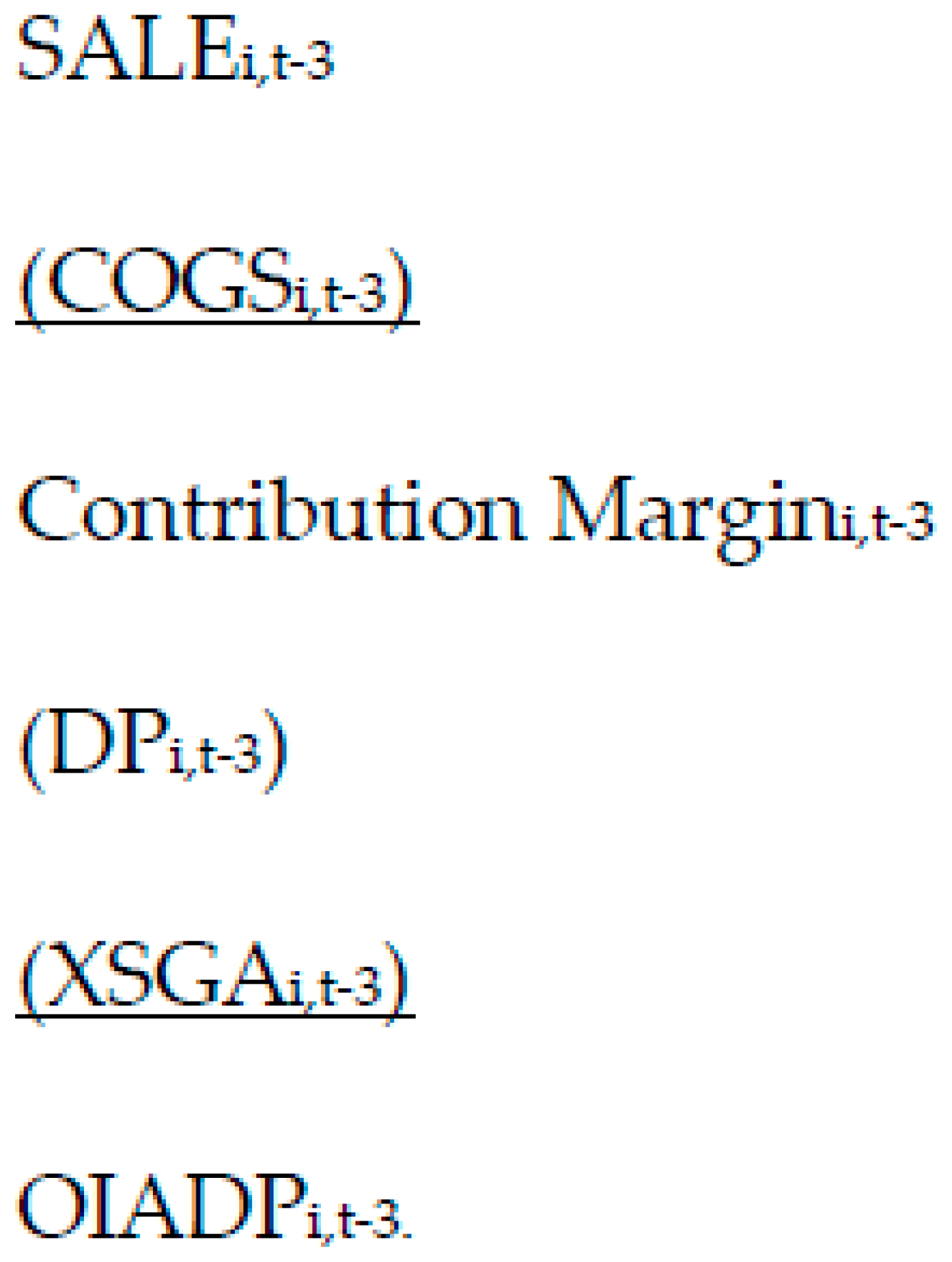
Table 2. Comparative Results for the Three Models of Operating Leverage.

Model	Linear Regression Results					Median Abs. Value Error
Model	N	Adj. R-square	Coeff	t-value	p-value	Median Abs. Value Error
BASE MODEL: No adjustment for constant SALE-to-COGS or sticky DP or XSGA [6]	241,106	0.015	0.121	61.415	0.000	40.40%
INTERMEDIATE MODEL: restated SALE-to-COGS but no adjustment for sticky DP or XSGA [9]	241,106	0.099	0.378	162.314	0.000	38.70%
FULL MODEL: adjustment for SALE-to-COGS and adjusting for sticky DP and XSGA as shown in Table 1 [11]	241,106	0.106	0.523	169.009	0.000	35.61%

Table 3. Predicting Next Quarter Operating Income (OIADP) Using the Full Model [11]. For 2005 Quarter 2 through 2021 Quarter 4. Where OIADP_i,t > 0 and OIADP_i,t-3 > 0.

Strata of Abs Value Errors	Count of Company-Years	Percent of Total Company-Years	Cumulative Percent of Company-Years	Percentiles of Company Years	Ordered Obs.	Percentile Abs Value Errors
0% to 5%	22,456	14.19%	14.19%	1st Percentile:	1,582	0.33%
5% and 10%	19,889	12.57%	26.76%	5th Percentile:	7,912	1.70%
10% and 15%	16,322	10.31%	37.08%	10th Percentile:	15,824	3.46%
15% and 20%	13,136	8.30%	45.38%	25th Percentile:	39,559	9.23%
20% and 25%	10,729	6.78%	52.16%	Median:	79,119	23.28%
25% and 50%	32,233	20.37%	72.53%	75th Percentile:	118,678	55.27%
50% and 100%	21,288	13.45%	85.98%	90th Percentile:	142,413	143.86%
> 100%	22,185	14.02%	100.00%	95th Percentile:	150,325	295.20%
Total:	158,238	100.00%	100.00%	99th Percentile:	156,655	1527.25%
Linear Regression Results
N		Adj R-square		Coeff	t-value	p-value
158,237		0.147		0.453	165.018	0.000

Table 4. Dow Jones Industrial Average (DJIA). Predicting Next Quarter Operating Income (OIADP) Using the Full Model [11]. Companies for Fiscal Quarters t from 2005 Quarter 2 through 2021 Quarter 4.

Strata of Abs Value Errors	Count of Company-Years	Percent of Total Company-Years	Cumulative Percent of Company-Years	Percentiles of Company Years	Ordered Obs.	Percentile Abs Value Errors
0% to 5%	380	20.42%	20.42%	1st Percentile:	19	0.24%
5% and 10%	341	18.32%	38.74%	5th Percentile:	93	1.32%
10% and 15%	276	14.83%	53.57%	10th Percentile:	186	2.46%
15% and 20%	184	9.89%	63.46%	25th Percentile:	465	6.15%
20% and 25%	145	7.79%	71.25%	Median:	930	13.84%
25% and 50%	319	17.14%	88.39%	75th Percentile:	1,395	27.60%
50% and 100%	107	5.75%	94.14%	90th Percentile:	1,674	55.22%
> 100%	109	5.86%	100.00%	95th Percentile:	1,767	110.55%
Total:	1,861	100.00%	100.00%	99th Percentile:	1,841	686.40%
Linear Regression Results
N		Adj R-square		beta	t-value	p-value
1,860		0.338		0.750	165.018	0.000

Table 5. All Company-Years. Predicting Next-Year Operating Income Using the Full Model [18]. Fiscal Years 2005 through 2021.

Strata of Abs Value Errors	Count of Company-Years	Percent of Total Company-Years	Cumulative Percent of Company-Years	Percentiles of Company Years	Ordered Obs.	Percentile Abs Value Errors
0% to 5%	19,400	10.28%	10.28%	1st Percentile:	1,888	0.48%
5% and 10%	17,613	9.33%	19.61%	5th Percentile:	9,439	2.45%
10% and 15%	15,155	8.03%	27.63%	10th Percentile:	18,878	4.87%
15% and 20%	12,899	6.83%	34.47%	25th Percentile:	47,194	13.24%
20% and 25%	10,770	5.71%	40.17%	Median:	94,389	36.15%
25% and 50%	34,904	18.49%	58.66%	75th Percentile:	141,583	97.33%
50% and 100%	32,026	16.97%	75.63%	90th Percentile:	169,899	264.52%
> 100%	46,010	24.37%	100.00%	95th Percentile:	179,338	536.49%
Total:	188,777	100.00%	100.00%	99th Percentile:	186,889	2760.82%
Linear Regression Results
N		Adj R-square		beta	t-value	p-value
188,776		0.064		0.259	113.678	0.000

Table 6. DJIA Company-Years Only. Predicting Next-Year OIADP Using the Full Model [18]. Fiscal Years 2005 through 2021.

Strata of Abs ERRORS	Count of Firm-Years	Percent of Total Firm-Years	Cumulative Percent of Firm-Years	Percentiles of Firm Years	Ordered Obs.	Percentiles of Abs. Value of Estimate Errors
0% to 5%	211	24.25%	24.25%	1st Percentile:	9	0.30%
5% and 10%	199	22.87%	47.13%	5th Percentile:	44	1.05%
10% and 15%	112	12.87%	60.00%	10th Percentile:	87	1.88%
15% and 20%	71	8.16%	68.16%	25th Percentile:	218	5.20%
20% and 25%	54	6.21%	74.37%	Median:	435	11.00%
25% and 50%	119	13.68%	88.05%	75th Percentile:	653	26.09%
50% and 100%	55	6.32%	94.37%	90th Percentile:	783	58.06%
> 100%	49	5.63%	100.00%	95th Percentile:	827	112.23%
Total:	870	100.00%	100.00%	99th Percentile:	861	475.18%
Linear Regression Results
N		Adj R-square		beta	t-value	p-value
869		0.354		0.936	21.846	<.001

Disclaimer/Publisher’s Note: The statements, opinions and data contained in all publications are solely those of the individual author(s) and contributor(s) and not of MDPI and/or the editor(s). MDPI and/or the editor(s) disclaim responsibility for any injury to people or property resulting from any ideas, methods, instructions or products referred to in the content.

© 2023 by the authors. Licensee MDPI, Basel, Switzerland. This article is an open access article distributed under the terms and conditions of the Creative Commons Attribution (CC BY) license (http://creativecommons.org/licenses/by/4.0/).

Copyright: This open access article is published under a Creative Commons CC BY 4.0 license, which permit the free download, distribution, and reuse, provided that the author and preprint are cited in any reuse.

Predicting Operating Income via a Generalized Operating Leverage Model

Abstract

Keywords:

Subject:

I. INTRODUCTION

II. BACKGROUND

III. METHODOLOGY

Data

Methodology for Predicting Quarterly OIADP

Restating Operating Leverage For Constant SALE / COGS Ratio For Quarters

Consideration of Dow Jones Industrial Average (DJIA) Firms

IV. RESULTS AND DISCUSSION

Results for Estimating Quarterly OIADP

Results for Estimating Annual OIADP

V. CONCLUSIONS, SUMMARY, AND FUTURE RESEARCH

Appendix A

Proof:

Appendix B

Applying ABJ Methodology to Compute Sticky Factors for XSGA and DP Quarterly

Appendix C

Notes

References

MDPI Initiatives

Important Links

Subscribe