Submitted:
07 November 2023
Posted:
08 November 2023
You are already at the latest version
Abstract
Financial time series and other human-driven, non-natural processes are known to exhibit fat-tailed outcome distributions. That is, such processes demonstrate a greater tendency for extreme outcomes than the normal distribution or other natural distributional processes would predict. We examine the mathematical expectation, or simply "expectation," traditionally the probability-weighted outcome, regarded since the seventeenth century as the mathematical definition of "expectation." However, when considering the "expectation" of an individual confronted with a finite sequence of outcomes, particularly existential outcomes (e.g., a trader with a limited time to perform or lose his position in a trading operation), we find this individual "expects" the median terminal outcome over those finite trials, with the classical seventeenth-century definition being the asymptotic limit as trials increase to this. Since such finite-sequence "expectations" often differ in values from the classic one, so do the optimal allocations (e.g., growth-optimal). We examine these for fat-tailed distributions. The focus is on implementation, and the techniques described can be applied to all distributional forms.
Keywords:
stopping times
; expectation
; finite sequences
; non-asymptotic
; optimal allocation
; Kelly criterion
; stable pareto
; fat tails
; generalized hyperbolic
MSC: 62E17; 62G32; 62L15; 62P05; 91A35; 91B28; 91B32
1. Introduction & Review of the Literature
In order to adequately apply methods of non-asymptotic expectation and allocation to stable Pareto distributed outcomes, we must examine the history of all three of these facets. First, we will review the history of fat-tailed distributions in economic time series, leading to the proposal of the Generalized Hyperbolic Distribution. Next, we will explore the history of mathematical expectation as well as optimal allocation methods which we will apply to stable Pareto distributed outcomes.
1.1. Fat-Tailed Distributions in Economic Time Series – History
While explicit mentions of fat-tailed distributions in financial price context may have been limited prior to the cited references, observations and discussions regarding market fluctuation irregularities and extreme event occurrences existed in financial history.
Historical examples like the financial crises and market panics occurring throughout history provide insights into understanding market dynamics and extreme event presence. Documented observations of events such as the 17th century Tulip Mania and 18th century South Sea Bubble offer glimpses into the irregular, non-normal behaviors exhibited in financial prices.
The field of speculative trading and risk management, with roots in ancient civilizations, involved assessing trading risks and managing uncertainties in commodity prices and exchange rates. While formal conceptualization of fat-tailed distributions may not have been explicitly articulated during these early periods, experiences and observations related to market irregularities and extreme price movements contributed to gradually understanding the complexities and non-standard behaviors present in financial markets and asset prices.
Exploring historical accounts of financial crises and the evolution of trading practices in ancient and medieval civilizations provides valuable insights into the early recognition of irregular market behaviors and consideration of extreme events in financial transactions and risk management.
One of the early explicit mentions of fat-tailed distributions in financial context is found in the work of economist Alfred Marshall. His contributions to supply-demand theory and goods pricing included discussions on market price variability and economic outlier occurrences. While Marshall’s work focused on microeconomic principles, his insights into market fluctuation nature provided preliminary understanding of heavy-tailed distribution potential presence in economic phenomena.
The field of actuarial science and insurance, predating modern finance theory, involved risk analysis and extreme event occurrence, laying foundations for understanding tail risk and accounting for rare but significant events in risk management.
While these earlier references did not explicitly focus on fat-tailed distributions in finance, they contributed to understanding variability and risk in economic/financial systems and provided insights leading to modern heavy-tailed distribution theories and finance applications.
Marshall's 1890 “Principles of Economics” [1] laid foundations for modern microeconomic theory and analysis. While focused on general economic principles, it included discussions on market dynamics, supply-demand, and price fluctuation factors.
Later, in his 1919 work “Industry and Trade” [2], Marshall examined industrial organization dynamics and market functioning, providing insights into price variability and factors influencing economic fluctuations.
Marshall's works provided insights into economic principles and market dynamics, laying groundwork for modern economic theory development. While not explicitly discussing finance-related fat-tailed distributions, they contributed to understanding market variability and economic analysis, providing context on risk and uncertainty ideas in economic systems.
Louis Bachelier’s 1900 thesis “Théorie de la spéculation” [3] delved into mathematical stock price modeling and introduced random walks, playing a significant role in efficient market hypothesis development and understanding financial price movements. While not focused on fat-tailed distributions, Bachelier's work is considered an early reference laying groundwork for understanding financial market stochastic processes.
The work of French mathematician Paul Lévy [4,5] made significant contributions to probability theory and stochastic processes, including those related to finance. Specifically, Lévy’s research on random variable addition and general stochastic processes greatly influenced modern probability theory development and understanding stochastic dynamics across fields. Lévy’s contributions to Brownian motion theory and introduction of Lévy processes provided groundwork for understanding asset price dynamics and modeling market fluctuations. Through foundational work on topics like Brownian motion, random processes, and stable distributions, Lévy helped establish mathematical tools and probability frameworks later applied to quantitative finance and modeling.
While explicit mentions of finance-related fat-tailed distributions may have been limited up to this time, Bachelier and Lévy’s contributions provided important insights into the probabilistic nature of finance and asset price movement governing processes.
By the 1950s, such distributional representations are appearing in the professional community, and the reader is referred to the reader is referred to https://nvlpubs.nist.gov/nistpubs/jres/77B/jresv77Bn3-4p143_A1b.pdf for a thorough expose on such distributional characteristics.
In Feller [6], we begin to find discussion of heavy-tailed distributions and their applications across fields. Although not explicitly mentioning stable Pareto distributions in finance-related context, Feller's work contributed to heavy-tailed distribution understanding.
Additionally, the notion of fat-tailed distributions in economics/finance was discussed by prominent statisticians and economists. Notably, Vilfredo Pareto [7] introduced the Pareto distribution in the early 20th century, closely related to the stable Pareto distribution, though may not have been directly applied to price data then.
The concept of stable Pareto distributions in finance context was notably introduced by mathematician Benoit Mandelbrot in his influential fractal and finance modeling work. Mandelbrot extensively discussed heavy-tailed distribution presence and implications for finance modeling.
In particular, Mandelbrot [8]discussed stable Pareto distributions as a potential model for certain financial data. This seminal paper laid foundations for his research on financial market fractal nature and non-Gaussian model applications describing market dynamics.
Additionally, Mandelbrot [9]expanded on these ideas, delving into stable distribution concepts and their significance in understanding market fluctuations and risk dynamics.
Differences between Pareto distribution, originally described by Vilfredo Pareto, and stable Pareto distribution, referred to by Benoit Mandelbrot in 1963 work, lie in their specific characteristics and properties.
The Pareto distribution, introduced by Vilfredo Pareto in early 20th century, is a power-law probability distribution describing wealth and income distribution in society. It exhibits a heavy tail, indicating a small number of instances with significantly higher values than the majority. It follows a specific mathematical form reflecting the “Pareto principle” or “80-20 rule,” suggesting roughly 80% of effects come from 20% of causes.
The stable Pareto distribution, referred to by Benoit Mandelbrot, represents an extension of the traditional Pareto distribution. Mandelbrot’s 1963 work marks a pivotal point in applying stable distributions, including stable Pareto, to financial data and market behavior modeling. It incorporates additional parameters allowing greater flexibility in modeling extreme events and heavy-tailed phenomena across fields like finance and economics. The stable Pareto distribution accounts for distribution shape and scale stability across scales, making it suitable for analyzing complex systems with long-term dependencies and extreme fluctuations.
While both distributions share heavy-tailed characteristics and implications for analyzing extremes and rarities, the stable Pareto distribution, as conceptualized by Mandelbrot, provided a more nuanced and adaptable framework for modeling complex phenomena, especially in finance and other dynamic systems where traditional distributions typically fell short capturing real-world data intricacies.
1.1.1. Symmetry in the stable Pareto
Regarding skewness, the stable Pareto distribution is generally considered to be symmetric, meaning that it does not exhibit skewness. However, modifications or specific applications of the stable Pareto distribution may allow for asymmetrical characteristics or variations in skewness to better accommodate the properties of the data being modeled. While the traditional stable Pareto distribution is symmetric, its extensions or adaptations can incorporate asymmetry if required to capture the underlying characteristics of the data more accurately. Often, in modeling financial price data or trading results, we are dealing with data which is lognormal.
1.1.2. The Stable Pareto Distribution and the Meaning of "Stable"
The stable Pareto distribution derives its name in part from the property of stability. In the context of this distribution, the term "stable" refers to the stability of the distribution's shape and scale parameters across different scales or time periods. More specifically, it implies that the statistical properties and characteristics of the distribution remain consistent and do not significantly change over time or as the scale of the data varies.
This stability concept signifies that the stable Pareto distribution retains its fundamental shape and scaling properties, even when subjected to data transformations, aggregation, or changes in data range. This feature is essential for capturing the heavy-tailed behavior and extreme value characteristics often observed in complex systems like financial markets. Here, the distribution parameters need to remain relatively constant to accurately represent the underlying data dynamics.
While "stable" does not mean the parameters are entirely fixed or immune to any changes, it does suggest the distribution exhibits a degree of robustness and resilience to variations in data scaling or time. This enables the stable Pareto distribution to reliably model rare events, extreme fluctuations, and long-term dependencies. It provides insights into tail event behaviors and their impacts on overall system dynamics.
1.1.3. Relationship to Stationarity
The "stable" terminology does not directly imply the stable Pareto distribution is stationary in the statistical sense. Rather, it primarily refers to the stability of the distribution's shape and scale parameters. This stability property relates to the distribution's resilience to transformations and scaling, allowing it to retain its fundamental shape and scaling properties under various conditions.
While not inherently associated with stationarity like some time series, the stable Pareto does exhibit certain stable shape and scaling characteristics. This provides a reliable framework for modeling heavy-tailed data and extremes in various domains including finance, risk management, and statistical analysis. However, for time-varying data or financial time series, additional assessments may be required to evaluate stationarity and determine appropriate modeling approaches for capturing data dynamics over time.
1.1.4. Accounting for Potential Non-Stationarity
The stable Pareto distribution itself is often considered stationary. However, in applications like financial markets or economic data, the data generating process may deviate from strict stationarity assumptions. Factors such as market shifts or underlying process changes could lead to variations in the stable Pareto parameters over time, making the distribution appear non-stationary in certain contexts.
In such cases, appropriate statistical tools and time series analysis techniques are essential to accurately assess data stationarity or non-stationarity. These tools can identify any time-dependent patterns, trends, or structural breaks that may affect the stability of the distribution. They enable informed decisions regarding suitable modeling and analysis approaches for the data characteristics and context. While generally associated with stationarity, the specific data properties and analysis objectives should determine the appropriate stable Pareto modeling framework.
Testing for non-stationarity in probability distributions, including the stable Pareto distribution, typically involves analyzing the statistical properties of the data to identify any time-dependent patterns, trends, or structural breaks that indicate a departure from stationarity. Several statistical tests and methods can be employed to assess non-stationarity in probability distributions depending on the nature of the data and the specific characteristics of interest. Some common approaches include Unit root tests (including the ADF test, for an exposition of results see [33]), Structural Break Tests, Time Series Decomposition, and Cointegration Analysis. (See Appendix A for a description of these.)
The jury is out as to whether economic data is stationary or not. Numerous papers have been written on the matter, and there are presently conflicting claims on the argument of stationarity in time series economic data. For our purposes, we shall assume stationarity, and point that in its absence, the same techniques may be employed after adjusting for non-stationarity.
1.1.5. Emergence of other fat-tailed distribution modeling techniques and the Generalized Hyperbolic Distribution (GHD)
With time, many other fat-tailed modelling techniques found their way into quantitative departments. The generalized hyperbolic distribution (GHD) had been introduced by [43]in examining aeolian processes.
The GHD constitutes a flexible continuous probability law defined as the normal variance-mean mixture distribution where the mixing distribution assumes the generalized inverse Gaussian form. Its probability density function can be expressed in terms of modified Bessel functions of the second kind, commonly denoted as BesselK functions in the literature. The specific functional form of the GHD density involves these BesselK functions along with model parameters governing aspects like tail behavior, skewness, and kurtosis. While not possessing a simple closed-form analytical formula, the density function can be reliably evaluated through direct numerical calculation of the BesselK components for given parameter values. The mathematical tractability afforded by the ability to compute the GHD density and distribution function underpins its widespread use in applications spanning economics, finance, and the natural sciences.
Salient features of the GHD include closure under affine transformations and infinite divisibility. The latter property follows from its constructability as a normal variance-mean mixture based on the generalized inverse Gaussian law. As elucidated by [44], infinite divisibility bears important connections to Lévy processes, whereby the distribution of a Lévy process at any temporal point manifests infinite divisibility. While many canonical infinitely divisible families (e.g. Poisson, Brownian motion) exhibit convolution-closure, whereby the process distribution remains within the same family at all times, Podgórski et al. showed the GHD does not universally possess this convolution-closure attribute.
Owing to its considerable generality, the GHD represents the overarching class for various pivotal distributions, including the Student's t, Laplace, hyperbolic, normal-inverse Gaussian, and variance-gamma. Its semi-heavy tail properties, unlike the lighter tails of the normal distribution, enable modeling of far-field behaviors. Consequently, the GHD finds ubiquitous applications in economics, particularly in financial market modeling and risk management contexts, where its tail properties suit the modeling of asset returns and risk metrics, and by 1995, the GHD appears in financial markets application in [34]. They applied the hyperbolic subclass of the GHD to fit German financial data.
This work was later extended by Prause in 1999 [35], who applied GHDs to model financial data on German stocks and American indices. Since then, the GHD has been widely used in finance and risk management to model a wide range of financial and economic data, including stock prices, exchange rates, and commodity prices. See [36], [37], [38], [39], [40], [41], [46], [42] for applications of the GHD to economic and share price data.
The GHD has been shown to provide a more realistic description of asset returns than the other classical distributional models, and has been used to estimate the risk of financial assets and to construct efficient portfolios in energy and stock markets.
The generalized hyperbolic distribution (GHD) has emerged as an indispensable modeling tool in modern econometrics and mathematical finance due to its advantageous mathematical properties and empirical performance. Salient features underscoring its suitability for analyzing economic and asset price data include:
- Substantial flexibility afforded by multiple shape parameters, enabling the GHD to accurately fit myriad empirically observed non-normal behaviors in financial and economic data sets. Both leptokurtic and platykurtic distributions can be readily captured.
- Mathematical tractability, with the probability density function, cumulative distribution function, and characteristic function expressible in closed analytical form. This facilitates rigorous mathematical analysis and inference.
- Theoretical connections to fundamental economic concepts such as utility maximization. Various special cases also share close relationships with other pivotal distributions like the variance-gamma distribution.
- Empirical studies across disparate samples and time horizons consistently demonstrate superior goodness-of-fit compared to normal and stable models when applied to asset returns, market indices, and other economic variables.
- Ability to more accurately model tail risks and extreme events compared to normal models, enabling robust quantification of value-at-risk, expected shortfall, and other vital risk metrics.
- Despite the lack of a simple analytical formula, the distribution function can be reliably evaluated through straightforward numerical methods, aiding practical implementation.
In summary, the mathematical tractability, theoretical foundations, empirical performance, and remarkable flexibility of the GHD render it exceptionally well-suited to modeling the non-normal behaviors ubiquitous in economic and financial data sets. Its rigor and applicability render it a standard apparatus in modern econometrics.
1.2. Mathematical Expectation – History
The genesis of mathematical expectation lies in the mid-17th century study of the "problem of points," which concerns the equitable division of stakes between players forced to conclude a game prematurely. This longstanding conundrum was posed to eminent French mathematician Blaise Pascal in 1654 by compatriot Chevalier de Méré, an amateur mathematician. Galvanized by the challenge, Pascal commenced a correspondence with eminent jurist Pierre de Fermat, and the two deduced identical solutions rooted in the fundamental tenet that a future gain's value must be proportional to its probability.
Pascal's 1654 work [10] compiled amidst his collaboration with Fermat, explores sundry mathematical concepts including foundational probability theory and expectation calculation for games of chance. Through rigorous analysis of gambling scenarios, Pascal delved into mathematical quantification of expected values, establishing core principles that seeded probability theory's growth and diverse applications. The "Pascal-Fermat correspondence" offers insights into the germination of mathematical expectation and its integral role in comprehending the outcomes of stochastic phenomena.
Contemporaneously in the mid-17th century, the Dutch mathematician, astronomer, and physicist Christiaan Huygens significantly advanced the field of probability and study mathematical expectation. Building upon the contributions of Pascal and Fermat, Huygens' 1657 [11] incisively examined numerous facets of probability theory, with particular emphasis on games of chance and the calculation of fair expectations in contexts of gambling. He conceived an innovative methodology for determining expected value, underscoring the importance of elucidating average outcomes and long-term behaviors of random processes.
Huygens' mathematical expectation framework facilitated subsequent scholars in expanding on his ideas to construct a comprehensive system for disentangling stochastic phenomena, quantifying uncertainty, and illuminating the nature of randomness across diverse scientific realms.
Essentially, the calculation for mathematical expectation, or "expectation" remained unchanged for centuries until [12]. It was Vince who decided to look at a different means of calculating it to reflect an individual or group of individuals who are in an "existential" contest of finite length. Consider a young trader placed on an institution's trading desk, and given a relatively short time span to "prove himself" or be let go, or the resources used by a sports team in an "elimination-style" playoff contest, or such resources of a nation state involved in an existential war.
Such endeavors require a redefinition of what "expectation" – what the party "expects" to have happen, and can readily be defined as that outcome where half the out-comes are better or the same and half are worse or the same at the end of the specified time period or number of trials.
Thus, the answer to this definition of "expectation" is no longer the classic, centuries-old definition of the probability-weighted mean outcome, but instead is the mean sorted cumulative outcome over the specified number of trials.
For example, consider the prospect of a game where one might win 1 unit with probability of .9, and lose -10 units with probability of .1. The classical expectation is to lose -0.1 per trial.
Contrast this to the existential contest which is only 1 trial long. Here, what one "expects" to happen is to win 1 unit. In fact, it can be shown that if one were to play and quit this game after 6 trials, one would "expect" to make 6 units (that is, half the out-comes of data distributed such would show better or same results, and half would show worse or same results.) After 7 trials, with these given parameters, however, the situation turns against the bettor.
Importantly, as demonstrated in [12], this non-asymptotic expectation converges to the asymptotic, centuries-old "classic" expectation in the limit as the number of trials approaches infinity. Thus, the "classic" expectation can be viewed as the asymptotic manifestation of Vince's more general non-asymptotic expression.
This redefined "expectation" then links to optimal resource allocations in existential contests. The non-asymptotic expectation provide a modern conceptualization of "expectation" tailored to modeling human behavior in high-stakes, finite-time scenarios, and, in the limit as the number of trials gets ever-large, converges on the classical definition of mathematical expectation.
1.3. Optimal Allocations – History
The concept of geometric mean maximization originates with Daniel Bernoulli, who made the first known reference to it in 1738. Prior to that time, there is no known mention in any language of even generalized optimal reinvestment strategies by merchants, traders, or in any of the developing parts of the earth. Evidently, no one formally codified the concept. If anyone contemplated it, they did not record it.
Bernoulli's 1738 paper [13]was originally published in Latin. A German translation appeared in 1896, and it was referenced in John Maynard Keynes' [14]. In 1936, John Burr Williams' [15] paper pertaining to trading in cotton, posited that one should bet on a representative price. If profits and losses are reinvested, the method of calculating this price is to select the geometric mean of all possible prices.
Bernoulli's 1738 paper was finally translated into English in Econometrica in 1954. When game theory emerged in the 1950s, concepts were being widely examined by numerous economists, mathematicians, and academics. Against this fertile backdrop, John L. Kelly Jr. [16] demonstrated that to achieve maximum wealth, a gambler should maximize the expected value of the logarithm of his capital. This is optimal because the logarithm is additive in repeated bets and satisfies the law of large numbers. In his paper, Kelly showed how Claude Shannon’s information theory [17] could determine growth-optimal bet sizing for an informed gambler.
Maximizing the expected end wealth is known as the Kelly criterion. Whether Kelly knew it or not, the cognates to his paper are from Daniel Bernoulli. In all fairness, Bernoulli was likely not the originator either. Kelly's paper presented this as a solution to a technological problem absent in Bernoulli's day.
Kelly's paper makes no reference to applying the methods to financial markets. The gambling community embraced the concepts, but applying them to various capital markets applications necessitated formulaic alterations, specifically scaling for the absolute value of worst-case potential outcome, which become particularly important given fat-tailed probabilities. In fairness, neither Kelly nor Shannon were professional market traders, and the work presented didn't claim applicability to finance. However, in actual practice, scaling to worst-case outcomes is anything but trivial1. The necessary scaling was provided in [18].
In subsequent decades after [16], many papers expanded on geometric growth optimization strategies in capital markets contexts by numerous researchers, notably Bellman, Kalaba [19], Breiman [20], Latane [21,22], Tuttle [22], Thorp [23,24] and others. Thorp, a colleague of Claude Shannon, developed a winning strategy for Blackjack using the Kelly Criterion and presented closed-form formulas to determine the Kelly fraction [23].
The idea of geometric mean maximization was also well-critiqued. Samuelson [26,27], Goldman [28], Merton [29] and others argued against universally accepting it as the investor criterion. Samuelson [26] highlighted the Kelly fraction is only optimal asymptotically, as the number of trials approaches infinity, not for finite trials, whereas, in fact, it would always be sub-optimal.
The formulation that yields the growth-optimal allocation to each component in a portfolio of multiple components for a finite number of trials is provided in [12]. This approach incorporates the net present value of amounts wagered and any cash flows over the finite timespan, acknowledging that real-world outcomes typically do not manifest instantly.
Growth-optimality, however, is not always the desired criterion. The formulaic framework for determining it can be used to discern other "optimal" allocations. In Vince & Zhu [30], we find two fractional allocations less than the growth optimal allocation for maximizing the various, catalogued, return-to-risk ratios. This is further expanded upon in de Prado, Vince, and Zhu [31].
Finally, [32] provides the case of using the formula for geometric growth maximization as a "devil's advocate" in contexts where the outcome from one period is a function of available resources from previous periods, and one wishes to diminish geometric growth. Examples include certain biological/epidemiological applications and "runaway" cost functions such as national debts.
2. Characteristics of the Generalized Hyperbolic Distribution (GHD) – Distributional Form and Corresponding Parameters
In addition to having the characteristics of being closed under affine transformations and possessing an infinitely divisible property which enables connections to Lévy processes, the GHD provides some practical implantation advantages to the study of economic data series. Among these, the GHD possesses:
- More general distribution class that includes Student's t, Laplace, hyperbolic, normal-inverse Gaussian, and variance-gamma as special cases. Its Mathematical tractability provides ability to derive other distribution properties.
- Exhibits semi-heavy tail behavior which allows modeling data with extreme events and fat-tailed probabilities.
- Density function involves modified Bessel functions of the second kind (BesselK functions). So although there is a lack of closed form density function, it can still be numerically evaluated in straightforward manner.
We examine the derivation of the Probability Density Function (PDF) of the symmetrical GHD, and then derive the first integral of the PDF with respect to the random variable to obtain the Cumulative Density Function (CDF) of the symmetrical GHD.
A characteristic function is a mathematical tool that provides a way to completely describe the probability distribution of a random variable. It is defined as the Fourier transform of the PDF of the random variable and is particularly useful for dealing with linear functions of independent random variables. We therefore derive the PDF of the symmetrical GHD Distribution:
1. Starting with the characteristic function of the symmetrical GHD Distribution, as derived from [45] as:
Where:
α = concentration
δ = scale
μ = location
λ = shape
γ = skewness
(Following now from [Bochner])…
2. Use the inversion formula: The PDF of the GHD can be obtained from the characteristic function using the inversion formula2:
3. Substituting the expression for the characteristic function into the Fourier inversion formula:
4. Simplifying the expression inside the exponential:
5. Using the identity to simplify the expression:
6. Substitute to simplify the integral:
7. Finally set the skewness parameter to zero to obtain the simplified PDF of the Symmetric GHD:
The derivation of the CDF of the symmetrical GHD follows:
1. Integrating the PDF from negative infinity to x to obtain the CDF:
2. Substituting the PDF into the integral and simplifying:
3. Substituting and to obtain:
4. With the identity to obtain:
5. Substituting and to obtain:
6. Finally, simplifying the expression by noting that and taking the limit as to obtain:
Where:
α = concentration
δ = scale
μ = location
λ = shape
= sign function, the sign of (x-u), or simply
Thus far, we have discussed the symmetrical GHD, where we are not accountable for skew (γ).
Implementing skew can become an unwieldy process in the GHD. Our focus is on implementation in this text, and the reader is reminded that although we present our work herein on the symmetrical GHD, it is applicable to all distributional forms, with the symmetrical GHD chosen so as to be current and relatively clear in terms of implementation of the techniques. It is the techniques that are important here -not so much the distributional form selected to demonstrate them herein. As such, the balance of the text will be using the symmetrical form of the GHD.
2.1 Parameter description
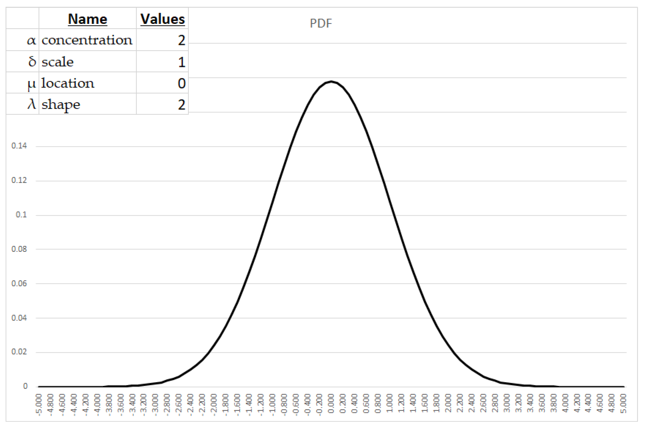
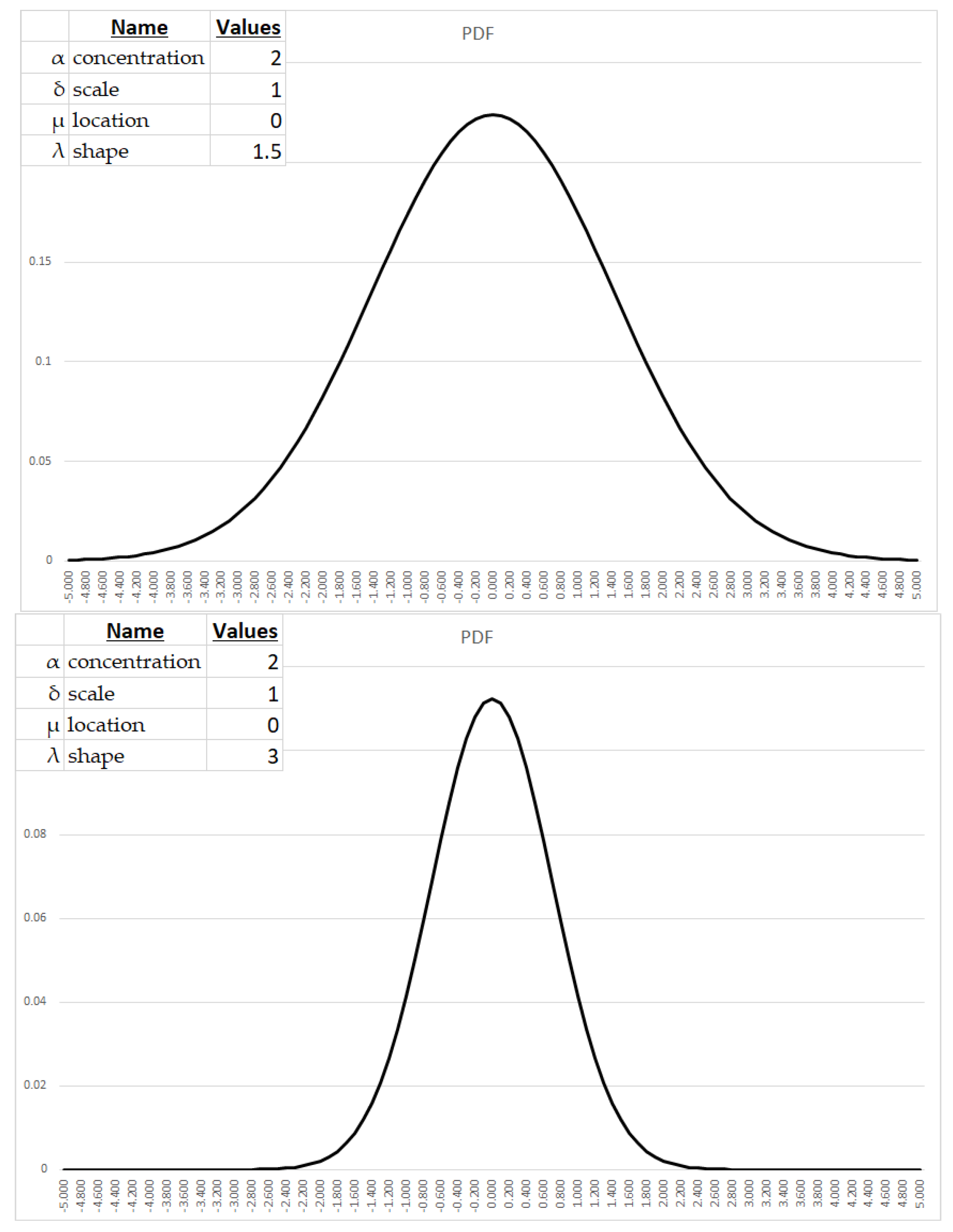
The symmetric generalized hyperbolic distribution (GHD) is parameterized by four variables governing salient distributional properties:
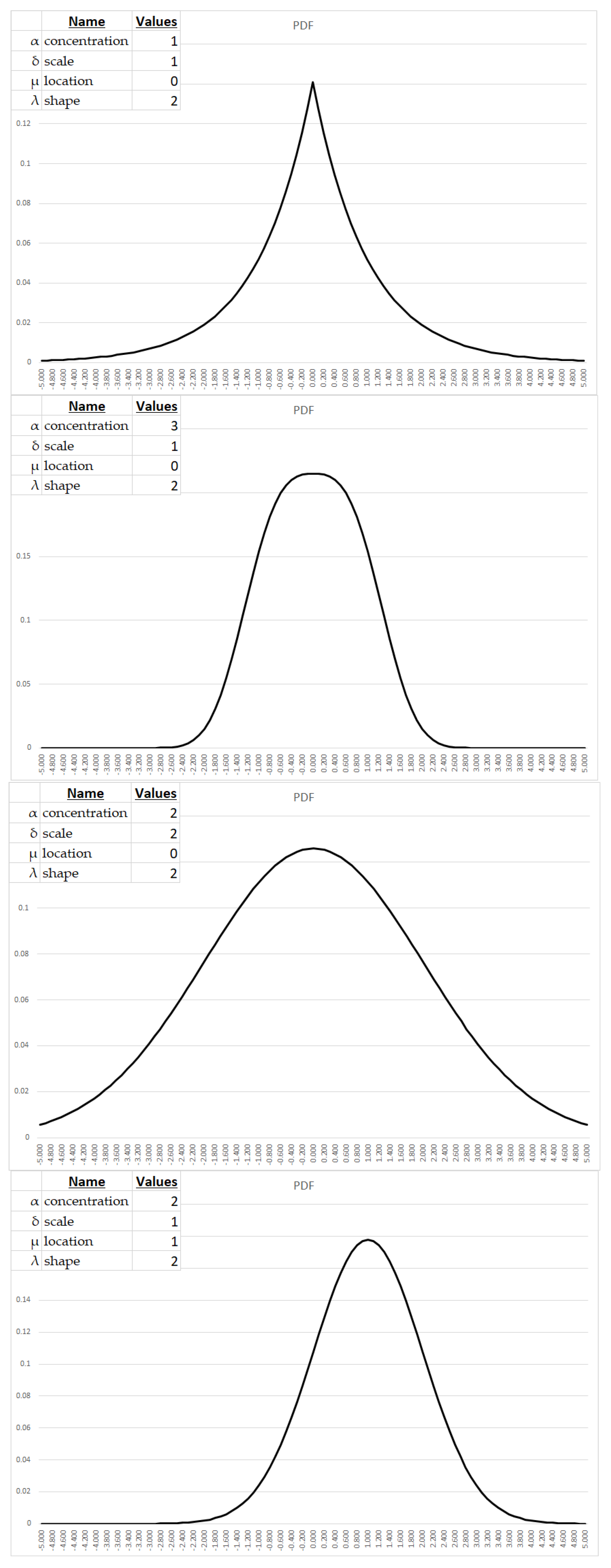
- The concentration parameter (α) modulates tail weight, with larger values engendering heavier tails and hence elevating the probability mass attributable to extreme deviations. α typically assumes values on the order of 0.1 to 10 for modeling economic phenomena.
- The scale parameter (δ) controls the spread about the central tendency, with larger values yielding expanded variance and wider dispersion. Applied economic analysis often utilizes δ ranging from 0.1 to 10.
- The location parameter (μ) shifts the distribution along the abscissa, with positive values effecting rightward translation. In economic contexts, μ commonly falls between -10 and 10.
- The shape parameter (λ) influences peakedness and flatness, with larger values precipitating more acute modes and sharper central tendencies. λ on the order of 0.1 to 10 frequently appears in economic applications.
While these indicated ranges provide first approximations, the precise parametric tuning warrants meticulous examination of the data properties and phenomenon under investigation. Moreover, complex interdependencies between the four variables potentially exist, necessitating holistic assessment when calibrating the symmetric GHD for applied modeling tasks.
In Appendix B we examine the basic form for the PDF and then amend the parameters to examine, graphically, the effects of each.
3. Parameter Estimation of the Symmetrical GHD
The task is now specified as follows. We have a set of empirical observations which represent the returns or percentage changes in an economic time series from one period to the next. This can be stock prices, economic data, the output of a trading technique3, or any other time-series data which comports to an assumed probability density function whose parameters we wish to fit to this sample data.
In the context of finding the concentration, scale, location, and shape parameters that best fit the PDF(x) or the symmetrical GHD, we can use Maximum Likelihood Estimation (MLE) to estimate these parameters.
Maximum likelihood estimation (MLE) is a common, well=known statistical method used to estimate the parameters of a probability distribution based on observed data. The method involves finding the parameter values that maximize the likelihood of observing the data given the assumed statistical model. MLE can be seen as a special case of the maximum a posteriori estimation (MAP) that assumes a uniform prior distribution of the parameters, or as a variant of the MAP that ignores the prior and which therefore is unregularized. The MLE estimator selects the parameter value which gives the observed data the largest possible probability (or probability density, in the continuous case). If the parameter consists of a number of components, then we define their separate maximum likelihood estimators, as the corresponding component of the MLE of the complete parameter. MLE is a consistent estimator, which means that as the sample size increases, the estimates obtained by the MLE approach the true values of the parameters if some conditions are met. In other words, as the sample size increases, the probability of getting the correct estimate of the parameters increases.
Mathematically, we can express MLE as follows:
1. Write down the likelihood function for the symmetrical GHD, which is the product of the PDF evaluated at each data point.
2. Take the natural logarithm of the likelihood function to obtain the log-likelihood function.
3. Take the partial derivative of the log-likelihood function with respect to each parameter and set the result equal to zero.
4. Solve the resulting system of equations to obtain the maximum likelihood estimates of the parameters.
5. Check the second-order conditions to ensure that the estimates are indeed maximum likelihood estimates.
6. Use the estimated parameters to obtain the best-fit symmetrical GHD.
In step 1, represents the vector of parameters to be estimated, which includes the concentration, scale, location, and shape parameters. In step 2, we take the natural logarithm of the likelihood function to simplify the calculations and avoid numerical issues. In step 3, we take the partial derivative of the log-likelihood function with respect to each parameter and set the result equal to zero to find the values of the parameters that maximize the likelihood function. In step 4, we solve the resulting system of equations to obtain the maximum likelihood estimates of the parameters. In step 5, we check the second-order conditions to ensure that the estimates are indeed maximum likelihood estimates. Finally, in step 6, we use the estimated parameters to obtain the best-fit symmetrical GHD.
By way of example now, we have a time-ordered vector of daily percentage changes in the S&P500 for the first six months of 2023.We assume these results as follows in Table 1:
We perform the MLE best-fit analysis now on our Returns sample data. One of the benefits of the GHD, as mentioned earlier, is the flexibility afforded by multiple shape parameters. We don’t necessarily have to fit per MLE or any other "best-fit" algorithm – we could fit by eye if we so desired, the GHD is that extensible. In our immediate case, we decided to fit but set the location parameter equal to the mean of our sample Returns (0.0029048), and fit the other three parameters, arriving at a best fit set of parameters in Table 2 as:
This results in the following PDF in Figure 1 and CDF in Figure 2 of our sample data set:
In working with the GHD it is often necessary to use the flexibility of the parameters in addition to a best-fit algorithm like MLE to obtain a satisfactory fit not only to the sample data, but to what the implementor may be anticipating in the future. Best-fit routines like MLE are, in actual practice, a starting point.
4. Discussion
This far we have laid the structural foundation to how we will use a given probability distribution and its parameters which are fitted to a sample set of data. The technique to be presented allows any distributional shape to be applied. We have chosen the symmetrical GHD for its ease-of-use. In actual practice it will be necessary to account for skewness in the distribution of the sampled data (this has been intentionally avoided in this paper to maintain simplicity)4.
Our focus is on finite sequences of outcomes from a stochastic process. (Although in our discussion, we are making the assumption that these outcomes are independent and identically distributed, IID, we assume this for simplicity of argument only; absent this IID assumption, the probabilities need only be amended at each subsequent trial in the finite, N-length sequence of outcomes based on previous outcomes.) We refer to these finite sequences as being "Existential Contests," realizing they exist in the milieu of life itself, as part of a longer sequence of a "lifetime-long" sequence of stochastic outcomes, or, in the milieu of many players confronted with a finite sequence of stochastic outcomes.
The gambler wandering through the casino does not see this sequence stop and start as it continues when he continues gambling.
These are "Existential Contests" because we are walling-off these principles of ultimate ergodicity. We are examining what the single, individual (in the context of one man, or one team, one nation state – all one "individual") player whose existence hangs on outcome of the N-length, finite sequence of outcomes; the milieu it resides in be damned. Examples of existential contests might include a young trader placed on an institution's trading desk, and given a relatively short time span to "prove himself" or be let go, or the resources used by a sports team in an "elimination-style" playoff contest, or such resources of a nation state involved in an existential war. Even our gambler wandering through a Las Vegas casino, placing the minimum sized bets, who, suddenly, decides to wager his life savings on numbers 1-24 at the roulette wheel before heading for the airport is now confronted with an N=1 existential contest.
The notion of existential contest does not fly in the face of The Optional Stopping Theorem5, which still applies in the limit as N gets ever-larger. The Theorem becomes less applicable as N approaches 0 from the right.
Not all human endeavors are regarded with the same, isotropic importance by the individual as traditional analysis assumes; some are more important than others, some are absolutely critical to the individual, deserving of analysis in its own, critical enclosure.
4.1 The goal of median-sorted outcome after N trials; the process of determining the representative "expected" setof oucomes
Let us return to our gambler in Las Vegas, ready to head for the airport, who decides to wager his life savings – half of it on the roulette ball falling on the numbers 1-12, "First Twelve" on the board, and the other half on 13-24, "Second Twelve," on the board. The payoff is 2:1. If the ball falls in any slot numbered 1-24, he will be paid 2:1 on one half of his life savings, keeping the half of his life savings wagered, and losing the other half. In effect, he has risked his entire life savings to increase it by half should the ball fall 1-24.
24 of the 38 slots will produce this result for him, so there is 24/38, or approximately 63.2% chance he will see a 50% increase in his life savings. On one, single play, what one expects is the median outcome, which in this case, given the .632 probability of winning, he "expects" to win6.
This is a critical notion here- what one "expects" to occur is that outcome, over N trials, where half of the outcomes after N trials are better, and half are worse. This is the definition of "expectation" in an existential contest.
However, it is always the expectation, as demonstrated in [12] in that, as N increases, this definition of expectation converges on the classical one accepted since the Seventeenth Century, as the sum of the probability-weighted outcomes. This "classical" definition of expectation is the expectation in the limit as the number of trials increases. Over a finite sequence of trials, the expectation is the median-sorted outcome which converges to the classic definition as the number of trials, N, gets ever greater. Thus, we can state, in all instances, the finite-sequence expectation is the actual expectation.
Examining this further, we find the divergence between the finite-sequence definition and the classical one is a function of skewness in the distribution of outcomes. Whereas the finite-sequence definition (expectation as median-sorted outcome) is always the correct "expectation" amount, regardless of N. The divergence between this result and the classical definition (the sum of the probability-weighted outcomes) is a function of skewness in the distribution of outcomes.
Most games of chance offer the player a probability <.5 of winning, with various payoffs depending on the players chances, even if the payoff is even money. However, in any game where the probability of profitability on a given play is <.5, and the classical expectation is negative, so too will the finite-sequence expectation be negative. Convergence is rapidly attained and never in the player's favor for any period of plays.
Earlier, we made reference to a hypothetical proposition where one might win 1 unit with probability of .9, and lose -10 units with probability of .1. The classical expectation is to lose -0.1 per trial.
This is in contrast to the existential contest which is only 1 trial long. Here, what one "expects" to happen is to win 1 unit. In fact, it can be shown that if one were to play and quit this game after 6 trials, one would "expect" to make 6 units (that is, half the outcomes of data distributed such would show better or same results, and half would show worse or same results.) After 7 trials, with these given parameters, however, the situation turns against the bettor.
We find similar situations arise in capital markets. It is not at all uncommon for commodity traders to employ trend-following models. Such models suffer during periods of price congestion and generally profit handsomely when prices break out and enter a trend. It is not at all uncommon for such approaches to see only 15% to 30% winning trades, yet, be profitable in the "long run." Thus, an investor in such programs would be wise to have as large an "N" as possible, the early phase of being involved in such an endeavor likely to be a losing one, yet, with something that would pay off well in the long run – as the finite period gets ever longer, the finite expectation converging on the classical one.
As we are discussing finite-length outcomes – "Existential Contests," we wish to:
- Determine what these finite-length expectations are, given a probability distribution we believe the outcomes comport to so as to base on our sample data and the fitted parameters of that distribution, -and-
- Determine a likely N-length sequence of outcomes for what we "expect," that is, a likely set of N outcomes representative of the outcome stream that would see half of the outcome streams of N length be better than, and half less than such a stream of expected outcomes. It is this "expected, representative stream" we will use as input to other functions such as determining growth-optimal allocations.
Regarding point #2, returning to our hypothetical game of winning one unit with p=.9, and losing 10 units otherwise. Here, the classical expectation is to lose 0.1 per play, with the finite expectation a function of N, and positive for the first 6 plays (assuming IID).
If one were to apply, say, the Kelly Criterion, which requires a positive classical expectation, one would wager nothing on such. However, this asymptotic assumption under the finite-period expectation is found to be precisely the opposite, which would have the player start out risking a "fraction" equal to 1.0.
4.2. Determining median-sorted outcome after N trials
4.2.1. Calculating the inverse CDF
To determine the median sorted outcome, we need to first construct the inverse CDF function. An inverse cumulative distribution function (inverse CDF) is a mathematical function that provides the value of the random variable for which a given probability has been reached. It is also referred to as the quantile function or the percent-point function. In simpler terms, the inverse CDF essentially allows you to determine the value at which a specified probability is attained in a given distribution.
To derive the inverse CDF of the Symmetrical GHD Distribution, we first start with the CDF of the Symmetrical GHD Distribution, which is given by:
Where:
α = concentration
δ = scale
μ = location
λ = shape
= sign function, the sign of (x-u), or simply
Rearranging the equation to isolate the term inside the curly braces:
We raise both sides to the power of :
Solving for :
Solving for :
The inverse CDF function takes a probability value as input and returns the corresponding value of such that:
Simplifying the expressions inside the parentheses:
Simplifying the expressions using the fact that :
This is our inverse CDF for the symmetrical GHD.
4.2.2. Worst-case expected outcome
Since we seek to construct a "representative" stream of outcomes, a stream of outcomes we would "expect" to be typical (half better, half worse) that what we would expect happen over N trials, and given the critical nature of "worst case outcome" in [18],[25],[30],[31],[12],[32] for which we wish to apply this expected stream of outcomes to, we thus wish to find that point on the distribution that we would expect be seen, typically, over N trials.
Using the inverse CDF, we can find this point, this "worst-case expected outcome" as that value of the inverse CDF for the input:
worst-case expected outcome = ( 1 / N ) N
We can use this to examine against the results of our representative stream of outcomes at the median sorted outcome.
4.2.3. Calculating the representative stream of outcomes from the median-sorted outcome
We proceed to discern the median sorted outcome. We will generate a large sequence of random variables (0..1) to process via our inverse CDF to give us the random outcomes from our distribution which we will take N at a time.
- For each of N outcomes, we determine the corresponding probability by taking the value returned by the inverse CDF as input to the CDF. When using the inverse CDF function, the random number generated is not the probability of the value returned by the inverse CDF. Instead, the random number generated is used as the input to the inverse CDF function to obtain a value from the distribution. This value is a random variable that follows the distribution specified by the CDF. To determine the probability of this value, you would need to use the CDF function and evaluate it at the value returned by the inverse CDF function. The CDF function gives the probability that a random variable is less than or equal to a specific value. Therefore, if you evaluate the CDF function at the value returned by the inverse CDF function, you will get the probability of that value.
- For our purposes however, we must now take any of these probabilities that are > .5 and take the absolute value of their difference to .5. Call this p`.
- p`= p if p <= .5
- p` = |1 - p| if p > .5
- c.
- We take M sets of N outputs, corresponding to outputs drawn from our fitted distribution as well as the corresponding p` probabilities.
- d.
- For each of these M sets of N outcome-p` combinations, we will sum the outcomes, and take the product of all of the p`s.
- e.
- We sort these M sets based on their summed outcomes.
- f.
- We now take the sum of these M product of p`s. We will call this the "SumOfProbabilities."
- g.
- For each M set, we proceed sequentially through them where each M has a cumulative probability specified as the cumulative probability of the previous M in the (outcome-sorted) sequence, plus the probability off that M divided by the SumOfProbabilities.
- h.
- It is this final calculation where we seek that M whose final calculation is closest to 0.5. This is our median sorted outcome, and the values for N which comprise it are our typical, median-sorted outcome, our expected, finite-sequence set of outcomes.
4.2.4. Example - calculating the representative stream of outcomes from the median-sorted outcome
We demonstrate the steps from 4.2.2 now. We will assume a finite stream of 7 outcomes in length (since we are using a distribution of daily S&P500 returns for the first half of 2023, we will assume we are modelling an existential contest of seven upcoming days in the S&P500). Thus, N=7.
We will calculate 1,000 such sets of these 7 outcomes, and therefore, M=1,000, and we therefore proceed to create, for each M, seven random values (0..1) representing the inputs to the inverse CDF, and the output for that N, then deriving the probability by taking the output for that N as input to the CDF. This final probability number we will process into a p`.
For each set of 7 probability-outcome pairs, we take the product of the p`s and the sum of the outcomes.

Table 3.
Sorted outcomes. Outcomes labelled as columns o1..o7, each row one of 1,000 of the M sets of N=7 outcomes.
Table 3.
Sorted outcomes. Outcomes labelled as columns o1..o7, each row one of 1,000 of the M sets of N=7 outcomes.
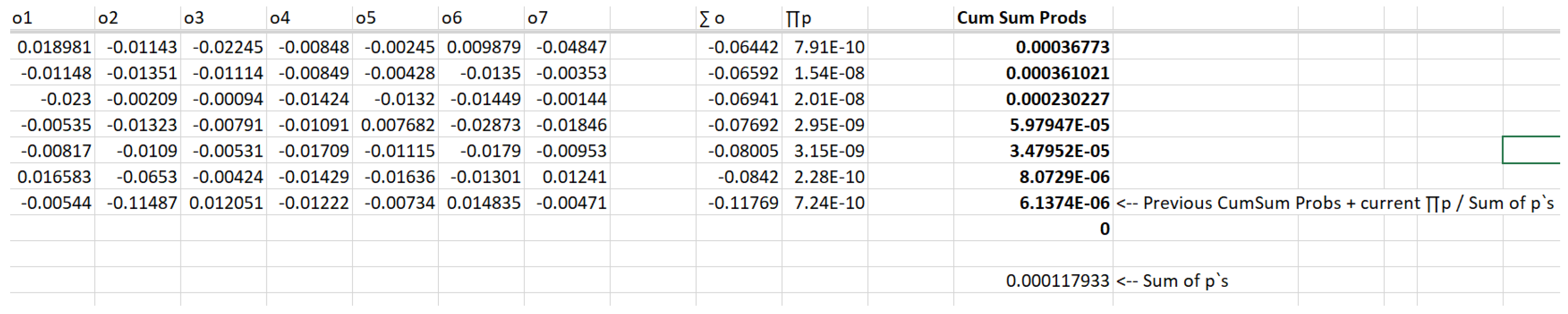
We next calculate the Cumulative Sum of the Probabilities for each M. This is simply the previous M in the sorted sequence, plus the p` product of the N p`s in the outcome-p` pairs, divided by the sum of such p`s over all M ("SumOfProbs").
Lastly, as shown in Table 4, we find that M in the sorted set of M sets that corresponds to a Cumulative Sum of Probabilities value closest to 0.5. This is the median sorted outcome. It's output values (o1..o7) represent the "typical" expected outcomes over N trials.
Table 4.
Sorted outcomes with median selected.
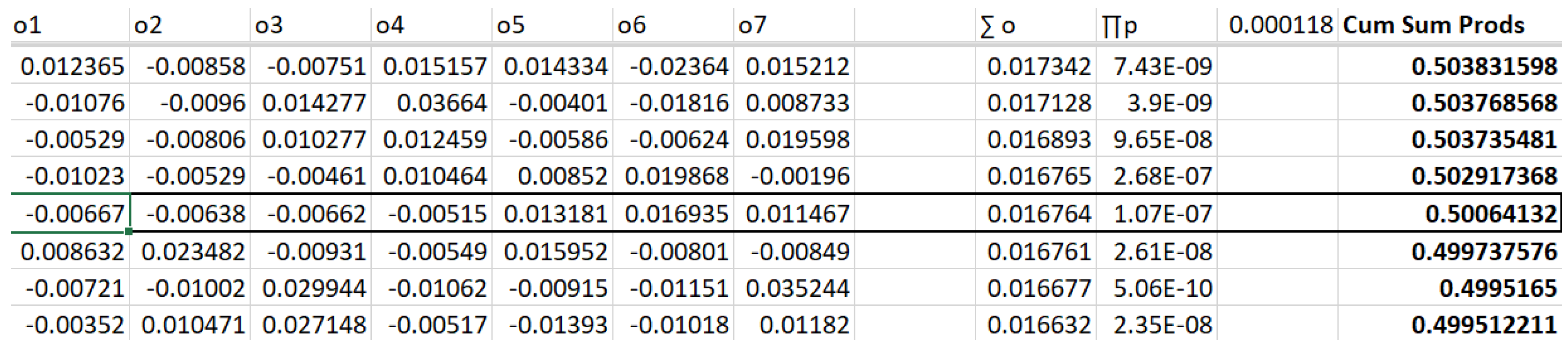
In this instance of 1,000 samples of sequences of N outcomes per the parameters for our symmetrical GHD representation of S&P500 closing percentage changes, we find the sample set, the "typical" set of seven closing prices – what we would expect, where half the time we would see a better sequence, half the time a worse one, as:
-0.006670152, -0.00638097, -0.006615831, -0.005151115, 0.013180558, 0.01693477, 0.011466985
Of note, our expected worst-case outcome we have calculated as -0.00642. As we have an outcome that is at least as negative as this, we are not deluding ourselves on what might be the worst-case outcome for the "typical," i.e., the median outcome stream of 7 outputs.
This setoff outcomes represents the expected, the typical set of outcomes from data distributed as the first half of 2023 for daily percentage changes in the S&P500.
Further, we can expect for 7 trials in this distribution of outcomes to see the ∑ o outcome of 0.016764 as our non-asymptotic expectation. Of note, we are using a symmetrical distribution in this paper and example, and as mentioned earlier, the divergence between the actual, finite expectation and the classical, asymptotic expectation is a function of the skewness of the distribution, which is 0 in our example. Nevertheless, the concept remains, the procedure illuminates this for more perverse and skewed distributions.
4.3 Optimal Allocations
4.3.1 Growth-optimal fraction
Earlier mention was made of determining the growth-optimal fraction from a sample data set, and how such results might diverge from the non-asymptotic determination of such.
Individuals and individual entities enmeshed in existential conflicts may very well be interested in finite-length growth optimization.
Consider, for a example, a proposition with p(.5) of winning 2 units versus losing 1 unit. Traditional (even by way of the Kelly Criterion, as the absolute value of the largest loss here is 1 unit) would determine asymptotic growth maximized by risking .25 of the stake on each play. However, when examined under the lens of finite-length, existential contests, terminal growth is maximized if the length of the contest is 1 play at a fraction of 1.0, and if N=2 plays, at a fraction of .5 per play, ad infinitum, to the asymptotic .25 risk of stake as N grows ever larger.
In determining optimal fractions of finite-length, existential contests, the input data (the values of -0.006670152, -0.00638097, -0.006615831, -0.005151115, 0.013180558, 0.01693477, 0.011466985 in our example, above) are what ought be used for determining the optimal fraction. For it is the data that determines the expectation in such finite-length trials that is the data germane to the also determining these other facets – the data one "expects" over those N trials, and seeking to maximize over.
4.3.2 Return/Risk Optimal Points
The amount to risk that is growth-optimal is return/risk optimal only asymptotically. For finite-length streams – existential contests, [30] demonstrates the two points on the spectrum of percentage risk which maximize the ratio of return to risk both as a tangent to the function on this spectrum as well as the inflection point "left" of the peak of the function.
Later, in [31] this is extended to determination of multiple, simultaneous contests (portfolios).
Particularly in determining these critical points of return/risk maximization, which are length-dependent, utilizing the input data that would be "expected" over such length of trials as demonstrated herein is more appropriate to the individual engaged in an existential contest.
4.3.3 Growth Diminishment in Existential Contests
In [32] a technique is presented whereby through examining an isomorphic mapping of the fraction to risk to the cosine of the standard deviation in percentage inputs to their arithmetic average, allows one to examine growth functions sans a "risk fraction," and instead in terms of variance in outcomes. The technique presented examined geometric growth functions where growth was a negative property. Such functions might be the cumulative debt of a nation, the growth of a pathogen in a population or within an individual organism, etc.
On the function plotted in terms of fraction of a stake to risk versus growth, as there is a growth optimal point, there is necessarily a point where the function begins decreasing and where growth goes negative by risking too much (for example, repeatedly risking beyond .5 in the 2:-1payoff game mentioned earlier with p(.9). One is certain to go broke as they continue to play risking .5 of their stake or more even in this very favorable game).
The isomorphic mapping provided in this paper allows one to examine such traits of the growth function without regard to the notion of a percentage of stake to risk, but rather of tweaking the variance.
As most endeavors to break malevolent growth function are inherently time-sensitive (i.e., of finite N – true "existential contests") the notion of using the median expected outcome stream over N trials is very germane to this exercise as well.
5. Conclusions
We are concerned with "individuals" (as one or a collection of individuals with a common goal) involved in finite-length sequences of stochastic outcomes – existential contests, where the distribution of such outcomes is characterized by fat-tails.
We have demonstrated how to fit an extensible, albeit symmetrical distribution to economic data series, and done so with techniques applicable to other distributional forms.
Once fitted, we demonstrate the process to determine the "expected" terminal outcome over the finite -length sequence, and the "expected" or "typical" outcomes that characterize such.
This is important in analyzing expectation of finite sequences, which differ from the classical expectation of the sum of the probability's times their outcomes, with the former being what is germane to the "individual" in an existential contest, whereby the former is always the correct expectation, one that approaches the classical one asymptotically.
Such "expectation," what the "individual" can "expect," as that which has half the outcomes better, half worse, also yields a typical stream of outputs achieving this expected outcome.
It is this stream of outputs which, to the individual in the existential contest, are the important inputs being they are what the individual "expects" for such finite-length calculations as growth-optional fractions, maximizing return to risk, or even for those whose charge is growth diminishment with a finite deadline, as life itself, despite the ever-present asymptotes, is rife with existential contests.
Funding
This research received no external funding.
Data Availability Statement
Data is also available upon request from the author.
Conflicts of Interest
The author declares that he has no conflicts of interest herein.
Appendix A
Common approaches to stationarity testing in series data:
- Unit Root Tests: Unit root tests, such as the Augmented Dickey-Fuller (ADF) test and the Phillips-Perron (PP) test, are widely used in time series analysis to assess the presence of a unit root in the data which indicates non-stationarity. These tests help determine whether the data series exhibits a stochastic trend or random walk behavior, indicating a lack of stationarity.
- Structural Break Tests: Structural break tests aim to detect significant shifts or changes in the statistical properties of the data at specific points in time. Techniques like the Chow test, the Quandt-Andrews test, and the Bai-Perron test are commonly employed to identify structural breaks and assess the presence of non-stationarity resulting from changes in underlying processes or regimes.
- Time Series Decomposition: Time series decomposition methods, such as trend analysis, seasonal adjustment, and filtering techniques, help separate the underlying components of the data series, allowing analysts to examine the trend, seasonality, and irregular fluctuations. Analyzing the behavior of these components can provide insights into the presence of non-stationarity and the dynamics of the data over time.
- Cointegration Analysis: Cointegration analysis is utilized to assess the long-term relationships between multiple time series variables. By examining the existence of cointegration relationships, analysts can determine whether the variables move together in the long run and whether the data series exhibit non-stationary behavior that is linked by a stable relationship.
These tests and techniques, among others, play a crucial role in identifying non-stationarity in probability distributions and time series data, enabling researchers and analysts to understand the dynamic nature of the data and make appropriate adjustments in the modeling and analysis of complex systems.
Appendix B
Here we shall examine the effect of changing individual parameters in the symmetrical GHD, while holding the others constant.
References
- Marshall, A. Principles of Economics; Macmillan and, Co., 1890. [Google Scholar]
- Marshall, A. Industry and Trade: A Study of Industrial Technique and Business Organization; Macmillan and Co., 1919. [Google Scholar]
- Bachelier, L. Théorie de la spéculation. Ann. Sci. De L'école Norm. Supérieure 1900, 17, 21–86. [Google Scholar] [CrossRef]
- Lévy, P. Théorie de l'addition des variables aléatoires; Gauthier-Villars: 1937.
- Kendall, D.G.; Levy, P.; Ito, K.; McKean, H.P.; Kimura, M. Processus Stochastiques et Mouvement Brownien. Biometrika 1966, 53, 293. [Google Scholar] [CrossRef]
- Feller, W. Theory of Probability; John Wiley & Sons: New York, NY, USA, 1950. [Google Scholar]
- Pareto, V. Pareto Distribution and its Applications in Economics. J. Econ. Stud. 1910, 5, 128–145. [Google Scholar]
- Mandelbrot, B. The Variation of Certain Speculative Prices. J. Bus. Univ. Chic. 1963. [CrossRef]
- Mandelbrot, B.; Hudson, R.L. The (Mis)Behavior of Markets: A Fractal View of Risk, Ruin, and Reward; Basic Books: New York, NY, USA, 2004. [Google Scholar]
- Pascal, B.; Fermat, P. Traité du triangle arithmétique. Corresp. Blaise Pascal Pierre De Fermat 1654, 2, 67–82. [Google Scholar]
- Huygens. 1657. Libellus de ratiociniis in ludo aleae (A book on the principles of gambling). (Original Latin transcript translated and published in English) London: S. KEIMER for T. WOODWARD, near the Inner-Temple-Gate in Fleet-street. 1714.
- Vince, R. Expectation And Optimal F: Expected Growth With And Without Reinvestment For Discretely-Distributed Outcomes Of Finite Length As A Basis In Evolutionary Decision-Making. Far East J. Theor. Stat. 2019, 56, 69–91. [Google Scholar] [CrossRef]
- Bernoulli, D. 1738. Specimen theoriae novae de mensura sortis (Exposition of a new theory on the measurement of risk). In Commentarii academiae scientiarum imperialis Petropolitanae 5: 175–192. Translated into English: L. Sommer. 1954. Econometrica 22: 23–36.
- Keynes, J.M. A Treatise on Probability; Macmillan: London, 1921. [Google Scholar]
- Williams, J.B. Speculation and the carryover. Q. J. Econ. 1936, 50, 436–455. [Google Scholar] [CrossRef]
- Kelly, J.L., Jr. A new interpretation of information rate. Bell Syst. Tech. J. 1956, 35, 917–926. [Google Scholar] [CrossRef]
- Shannon, C.E. A mathematical theory of communication. Bell Syst. Tech. J. 1948, 27, 379–423. [Google Scholar] [CrossRef]
- Vince, R. Portfolio Management Formulas; John Wiley & Sons, Inc.: New York, 1990. [Google Scholar]
- Bellman, R.; Kalaba, R. On the role of dynamic programming in statistical communication theory. IEEE Trans. Inf. Theory 1957, 3, 197–203. [Google Scholar] [CrossRef]
- Breiman, L. Optimal gambling systems for favorable games. In Proceedings of the fourth Berkeley symposium on mathematical statistics and probability, Jerzy Neyman; University of California Press: Berkeley, 1961; pp. 65–78. [Google Scholar]
- Latané, H.A. Criteria for Choice Among Risky Ventures. J. Politi-Econ. 1959, 67, 144–155. [Google Scholar] [CrossRef]
- Latane, H.; Tuttle, D. Criteria for portfolio building. J. Financ. 1967, 22, 362–363. [Google Scholar] [CrossRef]
- Thorp Edward, O. Beat the Dealer: A Winning Strategy for the Game of Twenty-One; Vintage: New York, 1962. [Google Scholar]
- Thorp, E. O. (1997; revised 1998). The Kelly Criterion in blackjack, sports betting, and the stock market. The 10th International Conference on Gambling and Risk Taking, Montreal, June 1997.
- Vince, Ralph. 1992. The Mathematics of Money Management. New York: John Wiley & Sons, Inc.
- Samuelson, P.A. 1971. The “fallacy” of maximizing the geometric mean in long sequences of investing or gambling. Proceedings of the National Academy of Sciences of the United States of America 68: 2493–2496. [CrossRef]
- Samuelson, P.A. Why we should not make mean log of wealth big though years to act are long. J. Bank. Finance 1979, 3, 305–307. [Google Scholar] [CrossRef]
- Goldman, M. A negative report on the ‘near optimality’ of the max-expected-log policy as applied to bounded utilities for long lived programs. J. Financial Econ. 1974, 1, 97–103. [Google Scholar] [CrossRef]
- Merton, R.C.; Samuelson, P.A. Fallacy of the log-normal approximation to optimal portfolio decision-making over many periods. J. Financ. Econ. 1974, 1, 67–94. [Google Scholar] [CrossRef]
- Vince, R.; Zhu, Q. Optimal betting sizes for the game of blackjack. J. Invest. Strat. 2015, 4, 53–75. [Google Scholar] [CrossRef]
- de Prado, M.L.; Vince, R.; Zhu, Q.J. Optimal Risk Budgeting under a Finite Investment Horizon. Risks 2019, 7, 86. [Google Scholar] [CrossRef]
- Vince, R. Diminution of Malevolent Geometric Growth Through Increased Variance. J. Econ. Bus. Mark. Res. 2020, 1, 35–53. [Google Scholar]
- Kim, J.H.; Choi, I. Unit Roots in Economic and Financial Time Series: A Re-Evaluation at the Decision-Based Significance Levels. Econometrics 2017, 5, 41. [Google Scholar] [CrossRef]
- Eberlein, E.; Ulrich, K. Hyperbolic distributions in finance. Bernoulli 1995, 1, 281–299. [Google Scholar] [CrossRef]
- Prause, K. The generalized hyperbolic model: Estimation, financial derivatives, and risk measures. PhD diss., University of Freiburg, 1999.
- Küchler, U.; Klaus, N. Stock Returns and Hyperbolic Distributions. ASTIN Bull. J. Int. Actuar. Assoc. 1999, 29, 3–16. [Google Scholar] [CrossRef]
- Eberlein, E.; Keller, U.; Prause, K. New Insights into Smile, Mispricing, and Value at Risk: The Hyperbolic Model. J. Bus. 1998, 71, 371–405. [Google Scholar] [CrossRef]
- Núñez-Mora, J.A.; Sánchez-Ruenes, E. Generalized Hyperbolic Distribution and Portfolio Efficiency in Energy and Stock Markets of BRIC Countries. Int. J. Financial Stud. 2020, 8, 66. [Google Scholar] [CrossRef]
- Selesho, J.M.; Naile, I. Academic Staff Retention As A Human Resource Factor: University Perspective. Int. Bus. Econ. Res. J. (IBER) 2014, 13, 295. [Google Scholar] [CrossRef]
- Zhang, J.; Fang, Z. Portfolio Optimization under Multivariate Affine Generalized Hyperbolic Distributions. Comput. Econ. 2022, 1–29. [Google Scholar] [CrossRef]
- Kostovetsky, J.; Betsy, K. Distribution Analysis of S&P 500 Financial Turbulence. J. Math. Financ. 2023. [Google Scholar] [CrossRef]
- Hu, C.; Anne, N.K. Risk Management with Generalized Hyperbolic Distributions. Glob. Financ. J. 2023. [Google Scholar]
- Barndorff-Nielsen, O. Exponentially decreasing distributions for the logarithm of particle size. Proc. R. Soc. London. Ser. A. Math. Phys. Sci. 1977, 353, 401–419. [Google Scholar] [CrossRef]
- Podgórski, K.; Wallin, J. Convolution-invariant subclasses of generalized hyperbolic distributions. Commun. Stat. - Theory Methods 2015, 45, 98–103. [Google Scholar] [CrossRef]
- Klebanov, L.; Rachev, S.T. The Global Distributions of Income and Wealth; Springer-Verlag: 1996.
- Klebanov, L.; Rachev, S.T. ν-Generalized Hyperbolic Distributions. J. Risk Financ. Manag. 2023, 16, 251. [Google Scholar] [CrossRef]
Figure 1.
PDF and CDF to fitted sample returns data from the first half of 2023 for the S&P500.
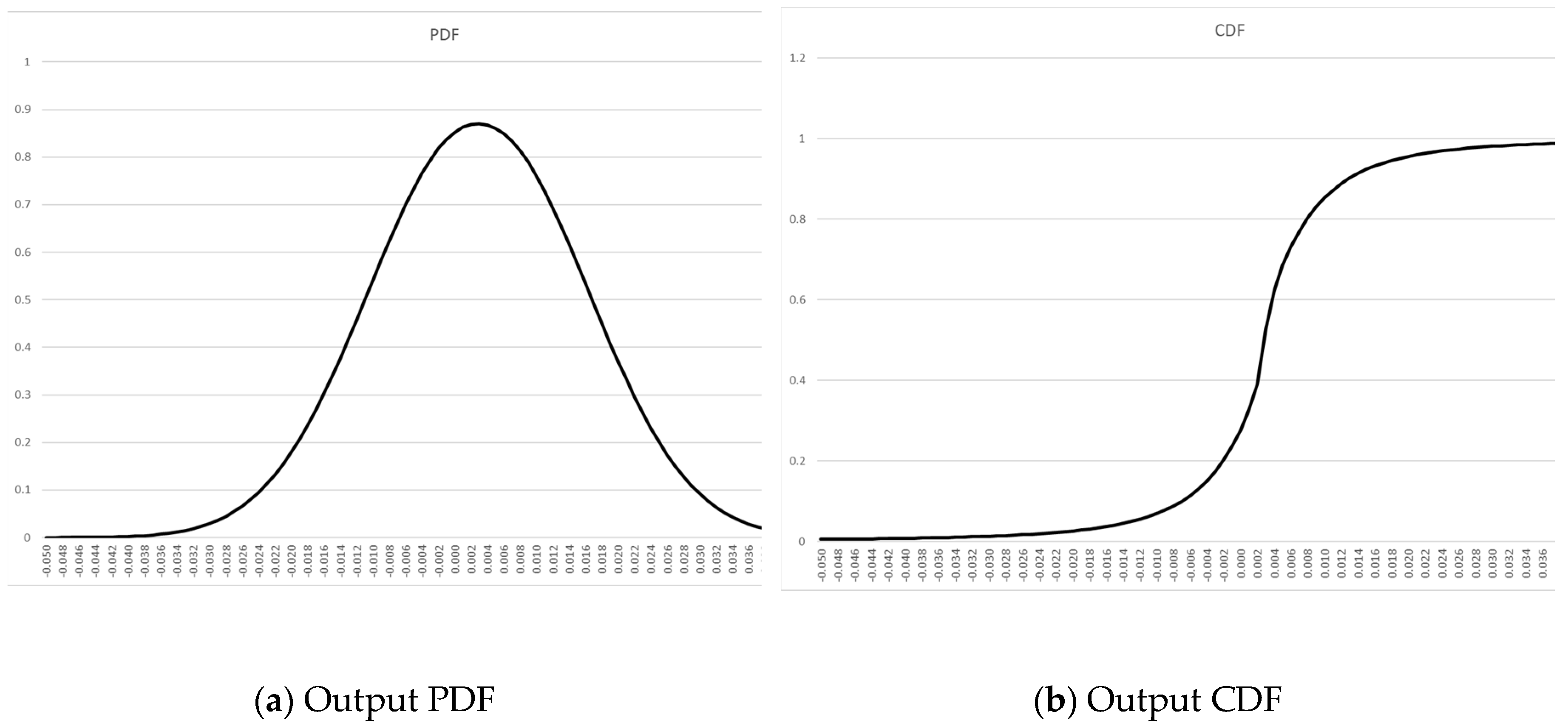
Table 1.
Daily percentage changes in the S&P500 for the first six months of 2023.
| Date | SP500 | % Change | Date | SP500 | % Change | |
| 20221230 | 3839.5 | 20230403 | 4124.51 | 0.003699 | ||
| 20230103 | 3824.14 | -0.004 | 20230404 | 4100.6 | -0.0058 | |
| 20230104 | 3852.97 | 0.007539 | 20230405 | 4090.38 | -0.00249 | |
| 20230105 | 3808.1 | -0.01165 | 20230406 | 4105.02 | 0.003579 | |
| 20230106 | 3895.08 | 0.022841 | 20230410 | 4109.11 | 0.000996 | |
| 20230109 | 3892.09 | -0.00077 | 20230411 | 4108.94 | -4.1E-05 | |
| 20230110 | 3919.25 | 0.006978 | 20230412 | 4091.95 | -0.00413 | |
| 20230111 | 3969.61 | 0.012849 | 20230413 | 4146.22 | 0.013263 | |
| 20230112 | 3983.17 | 0.003416 | 20230414 | 4137.64 | -0.00207 | |
| 20230113 | 3999.09 | 0.003997 | 20230417 | 4151.32 | 0.003306 | |
| 20230117 | 3990.97 | -0.00203 | 20230418 | 4154.87 | 0.000855 | |
| 20230118 | 3928.86 | -0.01556 | 20230419 | 4154.52 | -8.4E-05 | |
| 20230119 | 3898.85 | -0.00764 | 20230420 | 4129.79 | -0.00595 | |
| 20230120 | 3972.61 | 0.018918 | 20230421 | 4133.52 | 0.000903 | |
| 20230123 | 4019.81 | 0.011881 | 20230424 | 4137.04 | 0.000852 | |
| 20230124 | 4016.95 | -0.00071 | 20230425 | 4071.63 | -0.01581 | |
| 20230125 | 4016.22 | -0.00018 | 20230426 | 4055.99 | -0.00384 | |
| 20230126 | 4060.43 | 0.011008 | 20230427 | 4135.35 | 0.019566 | |
| 20230127 | 4070.56 | 0.002495 | 20230428 | 4169.48 | 0.008253 | |
| 20230130 | 4017.77 | -0.01297 | 20230501 | 4167.87 | -0.00039 | |
| 20230131 | 4076.6 | 0.014642 | 20230502 | 4119.58 | -0.01159 | |
| 20230201 | 4119.21 | 0.010452 | 20230503 | 4090.75 | -0.007 | |
| 20230202 | 4179.76 | 0.014699 | 20230504 | 4061.22 | -0.00722 | |
| 20230203 | 4136.48 | -0.01035 | 20230505 | 4136.25 | 0.018475 | |
| 20230206 | 4111.08 | -0.00614 | 20230508 | 4138.12 | 0.000452 | |
| 20230207 | 4164 | 0.012873 | 20230509 | 4119.17 | -0.00458 | |
| 20230208 | 4117.86 | -0.01108 | 20230510 | 4137.64 | 0.004484 | |
| 20230209 | 4081.5 | -0.00883 | 20230511 | 4130.62 | -0.0017 | |
| 20230210 | 4090.46 | 0.002195 | 20230512 | 4124.08 | -0.00158 | |
| 20230213 | 4137.29 | 0.011449 | 20230515 | 4136.28 | 0.002958 | |
| 20230214 | 4136.13 | -0.00028 | 20230516 | 4109.9 | -0.00638 | |
| 20230215 | 4147.6 | 0.002773 | 20230517 | 4158.77 | 0.011891 | |
| 20230216 | 4090.41 | -0.01379 | 20230518 | 4198.05 | 0.009445 | |
| 20230217 | 4079.09 | -0.00277 | 20230519 | 4191.98 | -0.00145 | |
| 20230221 | 3997.34 | -0.02004 | 20230522 | 4192.63 | 0.000155 | |
| 20230222 | 3991.05 | -0.00157 | 20230523 | 4145.58 | -0.01122 | |
| 20230223 | 4012.32 | 0.005329 | 20230524 | 4115.24 | -0.00732 | |
| 20230224 | 3970.04 | -0.01054 | 20230525 | 4151.28 | 0.008758 | |
| 20230227 | 3982.24 | 0.003073 | 20230526 | 4205.45 | 0.013049 | |
| 20230228 | 3970.15 | -0.00304 | 20230530 | 4205.52 | 1.66E-05 | |
| 20230301 | 3951.39 | -0.00473 | 20230531 | 4179.83 | -0.00611 | |
| 20230302 | 3981.35 | 0.007582 | 20230601 | 4221.02 | 0.009854 | |
| 20230303 | 4045.64 | 0.016148 | 20230602 | 4282.37 | 0.014534 | |
| 20230306 | 4048.42 | 0.000687 | 20230605 | 4273.79 | -0.002 | |
| 20230307 | 3986.37 | -0.01533 | 20230606 | 4283.85 | 0.002354 | |
| 20230308 | 3992.01 | 0.001415 | 20230607 | 4267.52 | -0.00381 | |
| 20230309 | 3918.32 | -0.01846 | 20230608 | 4293.93 | 0.006189 | |
| 20230310 | 3861.59 | -0.01448 | 20230609 | 4298.86 | 0.001148 | |
| 20230313 | 3855.76 | -0.00151 | 20230612 | 4338.93 | 0.009321 | |
| 20230314 | 3919.29 | 0.016477 | 20230613 | 4369.01 | 0.006932 | |
| 20230315 | 3891.93 | -0.00698 | 20230614 | 4372.59 | 0.000819 | |
| 20230316 | 3960.28 | 0.017562 | 20230615 | 4425.84 | 0.012178 | |
| 20230317 | 3916.64 | -0.01102 | 20230616 | 4409.59 | -0.00367 | |
| 20230320 | 3951.57 | 0.008918 | 20230620 | 4388.71 | -0.00474 | |
| 20230321 | 4002.87 | 0.012982 | 20230621 | 4365.69 | -0.00525 | |
| 20230322 | 3936.97 | -0.01646 | 20230622 | 4381.89 | 0.003711 | |
| 20230323 | 3948.72 | 0.002985 | 20230623 | 4348.33 | -0.00766 | |
| 20230324 | 3970.99 | 0.00564 | 20230626 | 4328.82 | -0.00449 | |
| 20230327 | 3977.53 | 0.001647 | 20230627 | 4378.41 | 0.011456 | |
| 20230328 | 3971.27 | -0.00157 | 20230628 | 4376.86 | -0.00035 | |
| 20230329 | 4027.81 | 0.014237 | 20230629 | 4396.44 | 0.004474 | |
| 20230330 | 4050.83 | 0.005715 | 20230630 | 4450.38 | 0.012269 | |
| 20230331 | 4109.31 | 0.014437 |
Table 2.
Best-fit parameter set to Table 1, only optimizing 3 parameters to the first 6 months in 2023 of daily S&P500 closing price changes. Location is set to the mean (and median, being symmetrical), of the sample data of 0.0029048 and scale we are simply keeping at the sample standard deviation of 0.0105381.
| Name | Values | |
|---|---|---|
| α | concentration | 2.1 |
| δ | scale | 0.01053813 |
| μ | location | 0.0029048 |
| λ | shape | 1.64940218 |
| 1 | It is this author's contention that Kelly and Shannon (who signed off on [16]) would have caught this oversight (they would not have intentionally opted to make the application scope of this work knowingly less general) had the absolute value of worst-case not simply been unity, thus cloaking it. |
| 2 |
n.b. In the characteristic function provided in the paper by Klebanov and Rachev (1996), t is a variable used to represent the argument of the characteristic function. It is not the same as , which is a variable used to represent the value of the random variable being modeled by the GHD.
The characteristic function of a distribution is a complex-valued function that is defined for all values of its argument . It is the Fourier transform of the probability density function (PDF) of the distribution, and it provides a way to calculate the moments of the distribution and other properties, such as its mean, variance, and skewness.
In the case of the GHD, the characteristic function is given by:
The argument of the characteristic function is a complex number that can take on any value. It is not the same as the value of the random variable being modeled by the GHD, which is represented by the variable . The relationship between the characteristic function and the PDF of the GHD is given by the Fourier inversion formula:
|
| 3 | These are often expressed as d0/d1 – 1, where d0 represents the most recent data, d1 the data from the previous period. In the case of outputs of a trading approach, the divisor is problematic; the results must be expressed in log terms, in terms of a percentage change. Such results must be expressed therefore in terms of an amount put at risk to assume such results, which are generalized to largest potential loss. The notion of "potential loss" is another Pandora's box worthy of a separate discussion. |
| 4 |
In actual implementation, we would use the full, non-symmetrical GHD. Deriving the PDF from the characteristic function of the GHD:
Starting with the characteristic function of the GHD:
Using the inversion formula to obtain the PDF of the GHD:
Substituting the characteristic function into the inversion formula and simplifing:
4. Changing variable :
5. Using the identity to simplify the integral:
This is the full PDF with the skewness parameter (γ) for the GHD.
The integral required to compute the CDF(x) of the GHD with skewness (γ) does not have a closed-form solution, so numerical methods must be used to compute the CDF(x). However, there are software packages such as R, MATLAB, or SAS that have built-in functions for computing the CDF(x) of the GHD. Once the CDF(x) is computed, the inverse CDF(x) can be obtained by solving the equation for , where is a probability value between 0 and 1. This equation can be solved numerically using methods such as bisection, Newton-Raphson, or the secant method. Alternatively, software packages such as R, MATLAB, or SAS have built-in functions for computing the inverse CDF of the GHD.
|
| 5 | This theorem states that, under certain conditions, the expected value of a martingale at a stopping time is equal to its initial value. A martingale is a stochastic process that satisfies a certain property related to conditional expectations. The Optional Stopping Theorem is an important result in probability theory and has many applications in finance, economics, and other fields. The theorem is based on the idea that, if a gambler plays a fair game and can quit whenever they like, then their fortune over time is a martingale, and the time at which they decide to quit (or go broke and are forced to quit) is a stopping time. The theorem says that the expected value of the gambler's fortune at the stopping time is equal to their initial fortune. The Optional Stopping Theorem has many generalizations and extensions, and it is an active area of research in probability theory. |
| 6 | In a European casino, he would have a better probability as there is only one green zero, and his probabilities therefore increase to 24/37, or approximately 64.9%. |
Disclaimer/Publisher’s Note: The statements, opinions and data contained in all publications are solely those of the individual author(s) and contributor(s) and not of MDPI and/or the editor(s). MDPI and/or the editor(s) disclaim responsibility for any injury to people or property resulting from any ideas, methods, instructions or products referred to in the content. |
© 2023 by the authors. Licensee MDPI, Basel, Switzerland. This article is an open access article distributed under the terms and conditions of the Creative Commons Attribution (CC BY) license (http://creativecommons.org/licenses/by/4.0/).
Copyright: This open access article is published under a Creative Commons CC BY 4.0 license, which permit the free download, distribution, and reuse, provided that the author and preprint are cited in any reuse.


