Submitted:
07 November 2023
Posted:
08 November 2023
You are already at the latest version
Abstract
Numerical simulations of standard situations in the transition region from gas kinetics to fluid dynamics at small Mach numbers indicate a clear dependence of the simulation results on the underlying kinetic model (here: nonlinear and linearized Boltzmann collision operator vs. BGK relaxation model). We develop an improved mathematical framework (trace theory) to explain these differences. In particular we reveal certain deficiencies for the classical BKG system as well as for the standard Navier Stokes approach.
Keywords:
Fluid dynamic limit
; kinetic models
; closure relations
; discrete velocity simulations
1. Introduction
Numerical simulations of flows in the transition from the gas kinetic (mesoscopic) to the fluid dynamic regime (macroscopic) represent a demanding task. On the mesoscopic side, the collision term operates on the 6-dimensional phase space and is very complex. On the macroscopic side, including a collision term in the fluid dynamic equations makes the problem become numerically stiff and hard to resolve in time.
In this situation simplyfying models are en vogue. The most popular ones are systems of BGK type which treat mesoscopic effects applying simple one- or more-parameter relaxation rules. Theoretical models try to find formulas from asymptotic analysis, taking into account the small mesoscopic perturbations as terms of an expansion with respect to some small parameter (Hilbert, Chapman-Enskog expansion). From this we find the Euler and the Navier Stokes equations as zeroth and first order approximations. Improved models, e.g. for a more detailed refinement of the pressure tensor are expected from higher order terms.
In the course of the present paper we demonstrate that all these models fail in certain practically relevant situations. E.g., the -expansion ansatz fails in some condensation-evaporation problem for a gas mixture (see section 6.2), leading to some unphysical ghost effect. The BGK ansatz yields systematic errors even in simple heat layer problems (section 6.1). In the following we propose a new ansatz (trace solutions) which works on the tangent space to the set of all Maxwellians (rather than the classical ansatz “solution=Maxwellian plus orthogonal perturbation”, supplemented with some exponential relaxation rule). As a motivation we discuss the relaxation of a simple local perturbation problem (see section 5.2). The crucial feature of the new approach is that (close to the fluid dynamic limit) the local macroscopic moments are not reflected by the local Maxwellian but by a specific moment perturbation.
The idea to construct intermediate states between arbitrary density functions and Maxwellians is not new. E.g. Shakhov [12] proposed such a system which is at present used for numerical simulations [14]. A comparable intention lies behind the idea of the extended BGK model with an additional relaxation parameter to match the correct Prandtl number. However, a better understanding of the transfer to fluid dynamics is not a question of parameter matching, and the above approaches do not yield a theoretical basis and a safe mathematical ground. Proposing a modified structure of kinetic solutions, the present paper claims to provide a new attempt to better understand the passage from the rarefied gas description to the macroscopic limit.
We derive closure relations which take the form of nonlinear first order (rather than second order) differential terms and thus are completely different from the parabolic second order terms of the Navier-Stokes system. The results allow to interpret the differences of various kinetic models (here: nonlinear and linearized Boltzmann collision operators and the BGK relaxation operator) in the fluid dynamical limit. As particular results we point at a purely nonlinear effect of the Boltzmann collision operator which is not reflected in the Navier-Stokes approach (section 5.3), and we demonstrate that the BGK system produces systematic artificial effects which are non-local and which do not vanish in the fluid dynamical limit (section 6.1).
The derivation of the trace ansatz requires some tedious mathematical arguments, which are necessary for a sufficient understanding of the mathematical framework. The technical part has been worked out in [5] (with Lea Bold as coauthor who has contributed the numerical results of section 5.3 which are crucial for the justification of the trace ansatz). In the present paper we have tried to shift the focus from the technical part to the applications (in particular section 6.2), while keeping the paper self-contained.
Having derived the trace ansatz, we have performed numerical simulation studies for testing and comparing the various models mentioned above. As a numerical tool we have used discrete velocity models (in the version as described in [3]) on - resp. -velocity grids which are sufficient in our cases. These are applicable in identical form for all of the discussed models. (To implement collision terms on grids in an efficient manner with valid flow parameters, the application of computer algebra tools is recommended, as demonstrated in [6] for the 2D case and [7] for the 3D case.) These systems are well-investigated, with systematic errors in numerical simulations being well-understood and under control [11]. Grids of the above size are preferrable mainly for small to moderate Mach numbers, creep flows, etc. The numerical results are in full agreement with the theoretical results.
The paper is organized as follows. Section 2 gives a short review over the abovementioned kinetic models. Section 3 introduces the general (non-closed) moment system derived from gas kinetics and derives the Euler system. Section 4 reinterprets the steps of the first order Chapman-Enskog approach for the Navier-Stokes system. In this way the central point of procedure can be generalized and becomes applicable to the full nonlinear collision operator without recourse to a formal series expansion. A new concept of balanced states is introduced, which are elements of the tangent space to the manifold of the Maxwellians and which replace (resp. supplement) the first order terms of the density function as provided by the Chapman-Enskog procedure. In Section 5 we introduce the concept of traces of kinetic solutions. Traces are comparable to projections of kinetic solutions onto the tangent spaces. The differential structure of the underlying dynamics provides a powerful tool to describe distributions in the neighborhood of Maxwellians. In order to keep the underlying ideas as concise and understandable as possible, we restrict theory and numerical examples one-dimensional geometries. Section 6 applies the results to the heat layer problem and discusses an evaporation condensation problem for gas mixtures.
2. Kinetic Models
The most fundamental kinetic model equation for a density function (x space-, velocity-parameter) of a single-species gas in phase space () is the classical Boltzmann equation
The Boltzmann collision operator is a bilinear operator integrating over all possible conservative two-particle collisions. It satisfies the conservation laws
The Boltzmann collision operator is ruled by the H-Theorem stating that in a space homogeneous environment all densities converge for to equilibrium functions e (these are functions satisfying ); all equilibrium functions are Maxwellians, i.e. functions of the form
uniquely determined by its macroscopic moments
In the following we denote by
the space of collision invariants, and by its orthogonal complement. We make use of the
(2.1) Decomposition Lemma:
Given a nonnegative density f and a Maxwellian e, there exists a unique decomposition
with M defined as
The decomposition takes the form
iff e has the same macroscopic moments as f.
- ( is a short hand notation for an element in , fully written as .)
Proof:
r can be uniquely determined by calculating mass, momenta and temperature on both sides. □
- The set of all Maxwellians is denoted by . Given , the tangent space in e is defined by
The full tangent space is the union
Two simplified alternatives to the nonlinear Boltzmann collision operator are the linearized collision operator and the BGL relaxation model. Both are based on the decomposition (3). Given , the Boltzmann collision operator is
Dropping the term which is quadratic in , we end up with the linearization of around e,
transfers f exponentially in time to its equilibrium e. The well-known properties of are as follows.
(2.2) The linearized collision operator:
Write . Then
- (a)
- (b) K is self-adjoint (e.g. in a weighted space) and negative semidefinite.
- (c) The restriction has an inverse .
- (d) The linear systemis solvable iff . In this case, the solution isIt satisfies
- The simplest kind of exponential decay of f to its equilibrium e is given by the one-parameter BGK model
- The solution of the linear system corresponding to (4) follows immediately from calculation.
(2.3) Linear system for BGK:
Suppose . The unique solution of
is
3. The moment hierarchy and the Euler system
Taking moments () of the Boltzmann equation or one of its models, and taking into account that for any of the above collision operators we end up with the following moment hierarchy.
- (3.4) General moment system:
- (3.5) Euler equations:
4. Navier-Stokes equations and balanced states
A prominent role in the refinement of the Euler system play the solutions (), and in of the linear equations
(For the solvability of the equations see (2.2)(c).)
- A convenient way to derive the Navier-Stokes system is the Chapman Enskog expansion of first order. Plugging the ansatzinto the Boltzmann equation and setting equal the terms of equal power of . For we findand thus . For we find
- For its solution we perform the decomposition (2) on the whole system. The part acting on readswith
- The solution of (19) is
- The Navier-Stokes correction to the Euler equations we now get by calculating the moment system (3.4) of the function . Taking into account the inequalities (6), we find the correction terms to the closure moments of the Euler system,with the positive viscosity resp. heat coefficients
- All the above results are classical and need no further explanation. Here, we find a way to reinterpret the Chapman Enskog results and to generalize them, without making use of the series expansion.
(4.6) Lemma: Let be a fixed Maxwellian and the corresponding flow term. The expansion of first order of Chapman-Enskog is the unique asymptotic solution () of the time-homogeneous initial value problem (IVP)
Proof: Decompose f uniquely into the form
Since and , we find
and solution of the IVP in ,
Since is invertible and negative definite, the asymptotics
exists and satisfies
Thus
- Thus the Chapman Enskog procedure as sketched above may be seen as a special case of the following three-step procedure for the calculation of closure relations.
(4.7) Scheme for closure relations:(1) Let and be given and fixed. Calculate a reduced discription of f containing all information concerning the relevant moments.
- (2) For an appropriate approximation C of the Boltzmann collision operator solve the IVP
(iii) Determine and calculate from this the closure relations for f.
- (In the Chapman-Enskog case, and .) We can interpret (22) as a local solution to the kinetic equation: Introduce a microscopic time scale and solve the kinetic system. In lowest order in , we freeze the source term at and solve the system for . In the following we call the distributions balanced states, since they balance the trend to equilibrium given by the collision operator with the perturbing effects produced by the streaming term.
5. Traces in tangent space
5.1. Traces
The definition of the linearized collision operator and the results of the above Chapman Enskog procedure above as well as the BGK model suggest a decomposition of f of the form (3) rather than (2). In this case, the central element e contains all macroscopic moments, but no contribution to the closure moments. In view of the balance equations described above with source term , we propose an alternative decomposition. For simplicity we restrict in the following to spatially one-dimensional problems (with space variable x) and with bulk velocities resp. .
- Given a triple with corresponding Maxwellian , the tangent space of in is defined as the set of all elements in
- (5.8) Closure relations for trace: The closure moments of the trace elements (in relation to the macroscopic moments , of ) are
We collect some results concerning the local structure of which can be proved by straightforward calculations and by Taylor expansion.
- (5.9) Differential structure of trace : (a) is differentiable with derivative
- Proof: (a) follows from straightforward calculations (using the definition (30) of and formulas (27), (28)) which yield
- For the derivation of closure moments for the nonlinear collision operator it is useful to follow the trace of along which is defined as the projection of given by
(5.10) Trace of nonlinear operator: (a) With ,
(b) Under the approximations of (5.9)(b),(c) for small ,
and the solution of the homogeneous trace Boltzmann equation
is in lowest order given by
Proof: (a) From the definition of (30) and the fact that follows
In a coordinate system centered around , is an even function with respect to . Thus
(b) follows from inserting the approximations (5.9)(b),(c).
- In our context, the most significant difference between the nonlinear collision operator on the one side, and the linearized and the BGK operator (shortly termed as “relaxation operators”) on the other side is that
5.2. Relaxation problems
Consider the initial value problem
with C one of the collision operators discussed above. Depending on , there exists a unique Maxwellian with the same macroscopic moments as , which is the asymptotic state of the solution for . In the relaxation case we have exponential decay to , (33), (34). The dynamics of the nonlinear solution is more detailed, depending on the form of .
- Suppose
Case 2 is more complex and we may recognize three phases. Phase I represents the relaxation of the perturbation to , phase II (“convex phase”) the transition from to , and phase III the exponential relaxation to . In the special case , phase II marks the transition of the trace element to . The slope of phase III is given by the parameter of (73). As a special feature we notice that the life time of the moment perturbation is much larger than for a model with relaxation rates based on the mean free path. The BGK model is not capable to cover this situation and we have to decide whether to match to the initial Maxwellian or the final Maxwellian, depending on whether we want to simulate the short-time or the long-time behaviour.
5.3. Relaxation with source, balanced states
In view of the equations to be solved for the closure relations let’s have a look on solutions of the equation with source,
and in particular their asymptotic states for (balanced states). For the relaxation systems we easily find
Both solutions satisfy the orthogonality relation
This is no surprise, since the source is even with respect to , and L maps even into even functions, while is odd. So it is remarkable to observe that orthogonality is not given for the nonlinear solution, as can be seen in Figure 2. (This observation was made in [8].) To understand this phenomenon, it helps to look at trace solutions. We easily see that is a balanced solution to the trace version of (36). However, it is not stable in the sense of dynamical systems, and there is another solution. Necessary and sufficient for balancing solutions is the orthogonality relation
resp.
which in leading order leads to
With we finally end up with
(5.11) Balanced state (Relaxation with source): Under the smallness assumptions for in (5.9) and with an appropriate constant , the leading order term of the stable solution is given by
The solution has an additonal contribution to the pressure tensor of the order as given in (58) .
- This example is an indicator that the concept of traces is relevant for the investigation of the structure of kinetic solutions in the context of closure relations. We can generalize the above principle to other sources and kinetic models.
(5.12) Balancing condition: Suppose given a source and a collision operator with traces
marks a balanced state if and only if the orthogonality condition
is satisfied which is equivalent to the balancing condition
6. Applications
6.1. Heat layers with zero flow
We consider the steady flow between two totally reflecting walls at different temperatures with a temperature difference . Since , the moment equations read
The closure moments for the solution are determined from the asymptotic solution for the model at hand of
In the Navier-Stokes description, contains no contribution to , and from equations ... we find the heat layer solution
Comparing the temperature profiles of numerical simulations for the nonlinear and the BGK system (Figure 3) we find that the BGK profile is considerably flatter than that of the nonlinear case. The latter one is close to the constant gradient profile (solid line) linearly connecting the wall temperatures. An explanation for th the difference is given by comparing the closure moments for both models (Figure 4). In Figure 4(a) we find a small almost constant contribution (maybe weakly dependent on the temperature) in the nonlinear case. Zooming into Figure 4(b) confirms this. However, for BGK we find a distinct, almost constant gradient over the whole field of calculation. An explanation for this is again provided by the trace description which allows to draw a rough picture pointing out the differences between nonlinear collision operator and BGK model. A full discussion of the trace solutions for both models in the fluid dynamic limit is provided in [5]. We do not repeat the tedious calculations of [5] but explain by a short argument why the BGK system does not provide the correct temperature gradient in the fluid dynamic limit. Suppose is the steady solution of the balance equation for the BGK system,
The first term on the left hand side represents in the limit a finite heat flux modeled by some term of the form . For small we may use the approximation (65) for shortly denoted as . Furthermore, yields an unknown contribution which comes out as a solvability condition for the above equation,
Its solution is
and
Thus under the above assumptions A is singular in the limit which is not realistic. The only way out is that c and with this B are -dependent and vanish in the limit. This explains qualitatively the flattened curve for the temperature profile of the BGK model. In the limit it is supposed to yield a constant temperature profile.
Remark: The results show that trace theory does not fit into the classical series expansion ansatz since it contains fractional powers of .
6.2. Gas mixtures: An evaporation condensation problem
The initial motivation for the present work came from the study of a gas mixture problem. The two-component gas consists of vapor (species A) which can evaporate or condensate at the flat confining walls of an infinite strip, and of some noncondensable component (species B) which is totally reflected (with energy exchange) at the walls. Given a pressure difference, the gas is attracted by one of the walls, and some portion of species A condenses, which results in a flow through the wall. Suppose there is only a small (almost neglegible amount of species B in the mixture. Calculating the fluid dynamic limit applying standard expansion techniques (here: Hilbert expansion) leads to a ghost effect: An infinitely thin boundary layer of the noncondensable completely cuts down the flux of species A, although in the limit the flow velocity of the ensemble is zero. Details of this example are described in [1] and the literature cited there. In [4] we have demonstrated that the reason for the confusion lies in some bifurcation structure of the solution space in the case of small velocities. We are now able to present the full solution to the above problem using the trace theory approach.
Deriving a trace theory for a gas mixture could closely follow the lines developed in the preceding sections.We will not do this here but restrict to a subproblem. We have numerically simulated the evaporation condensation problem and ended up with results part of which is given in Figure 5. Here we find some boundary layer close to the left wall (which is large scale and thus not a kinetic boundary layer).Far apart from the wall the whole ensemble seems to tend to some equilibrium state. This cannot be a common Maxwellian, since Species A and B exhibit different velocities and temperatures. Such an equilibrium state does not exist in classical theory. However, trace theory approach results in a common balanced state of the mixture far on the right of the perturbing wall. In particular, we find the dependence of the condensation rate for A on the interaction between both species, and on the energy exchange of species B on the left wall. Here, we roughly sketch the corresponding calculations.
Suppose the restrictions and to their species have moments and with corresponding Maxwellians and . Constructing we assume that both and are trace elements of their respective Maxwellians, and with corresponding parameters given by formulas (54) and (55),
Compatibility conditions are the equalities and , i.e.
These fix once is given, and the temperature difference in relation to the velocity of A. Both trace elements are now represented by and perturbations of the same Maxwellian .
Let a nonlinear two-species collision operator be given as
with restrictions to the species being
The operators and are the usual one-species collision operators, while and represent the interspecies interactions. The above trace construction is a balanced solution with respect to this operator, if it satisfies the balance conditions
where the closure moments have to be taken relative to their corresponding bulk velocities . From this we extract conditions of the form
with and positive constants to be derived from the collision operator. (For compare (71). can be derived similarly from the interspecies operators.). From the first condition we can calculate , the second one relates the velocity to the temperature .
References
- K. Aoki, S. K. Aoki, S. Takata, and S. Taguchi. Vapor flows with evaporation and condensation in the continuum limit: effect of a trace of noncondensable gas. Eur. Journ. Mech. B/Fluids, 2003; 71. [Google Scholar] [CrossRef]
- H. Babovsky. A numerical model for the Boltzmann equation with applications to micro flows. Comput. Math. Appl. 2009. [CrossRef]
- H. Babovsky. Discrete kinetic models in the fluid dynamic limit. Computers and Mathematics with Applications, 2014. [CrossRef]
- H. Babovsky. Macroscopic limit for an evaporation-condensation problem. European Journal of Mechanics B/Fluids, 2017. [CrossRef]
- H. Babovsky and L. Bold. Balanced states and closure relations: The fluid dynamic limit of kinetic models. 2022. [CrossRef]
- H. Babovsky and J. Grabmeier. Calculus and design of discrete velocity models using computer algebra. 1786. [CrossRef]
- H. Babovsky and J. Grabmeier. A Symmetry Class Approach to 3D Discrete Collision Models via Computer Algebra, 2022.
- L. Bold. Diskrete Geschwindigkeitsmodelle und ihr Bezug zu den Navier-Stokes-Gleichungen. 2022.
- C. Cercignani. The Boltzmann equation and its applications. 1988.
- C. Cercignani, R. C. Cercignani, R. Illner and M. Pulvirenti. The Mathematical Theory of Dilute Gases. 1994. [Google Scholar]
- T. Sasse. Discrete Velocity Models for Mixtures and Non-Mixtures, 2021.
- E.M. Shakhov. Fluid Dynam. 1968.
- Y. Sone. Molecular Gas Dynamics. 2007.
- V. A. Titarev. Application of model kinetic equations to hypersonic rarefied gas flows. Computers & Fluids, 2018. [CrossRef]
Figure 1.
Relaxation of random initial perturbation. (a) , (b) .
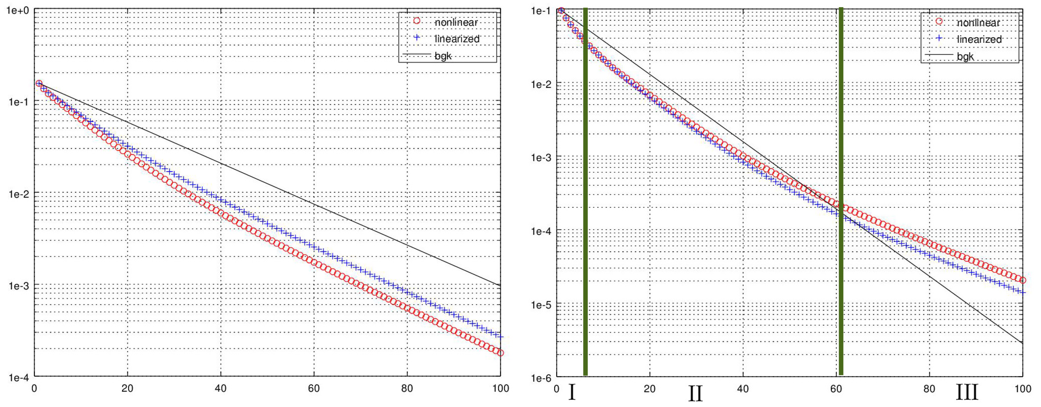
Figure 2.
Evolution of scalar product of IVP (36), nonlinear and linearized Boltzmann collision operator.
Figure 2.
Evolution of scalar product of IVP (36), nonlinear and linearized Boltzmann collision operator.
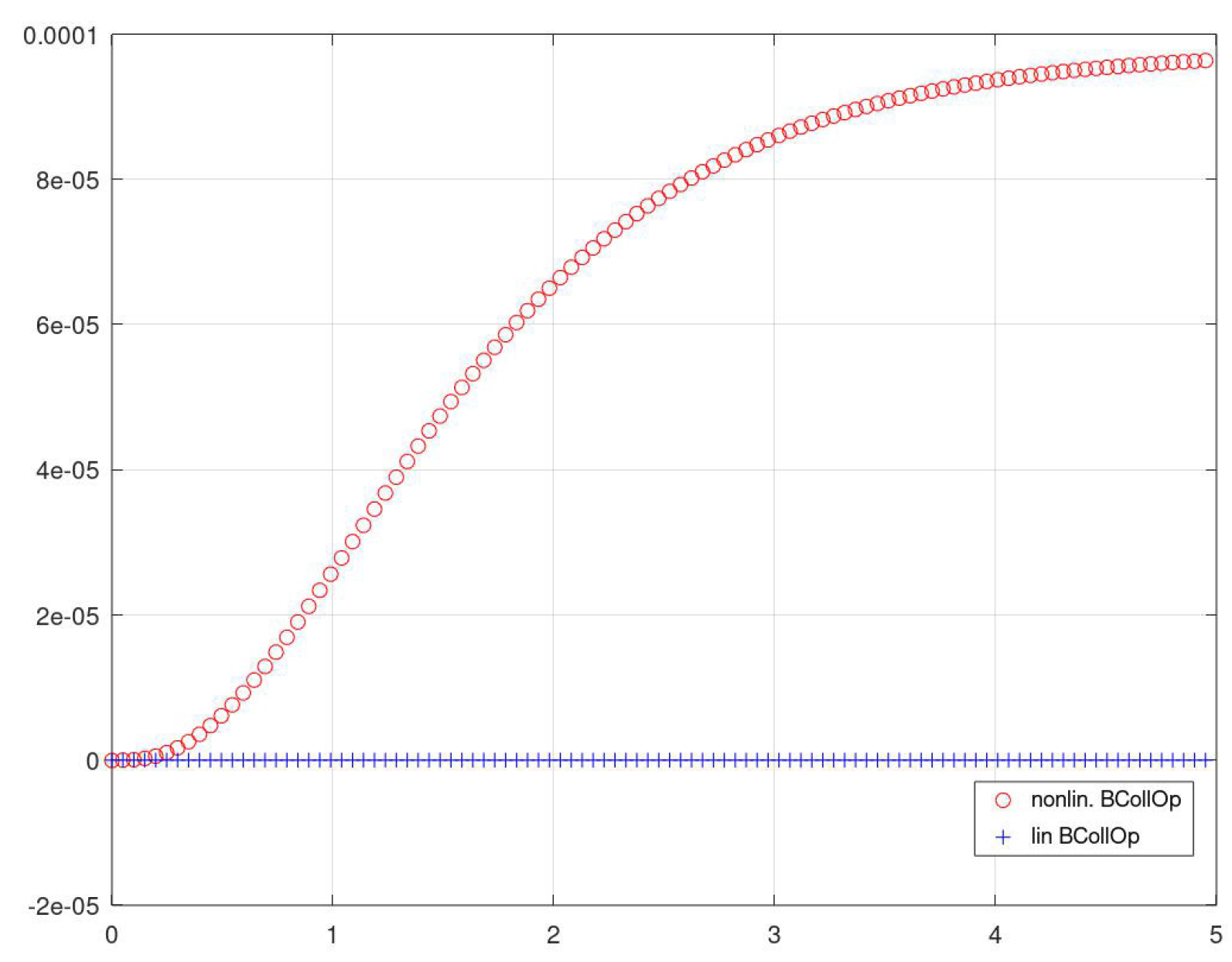
Figure 3.
Heat layer for nonlinear collision operator and BGK model. Temperature profiles.
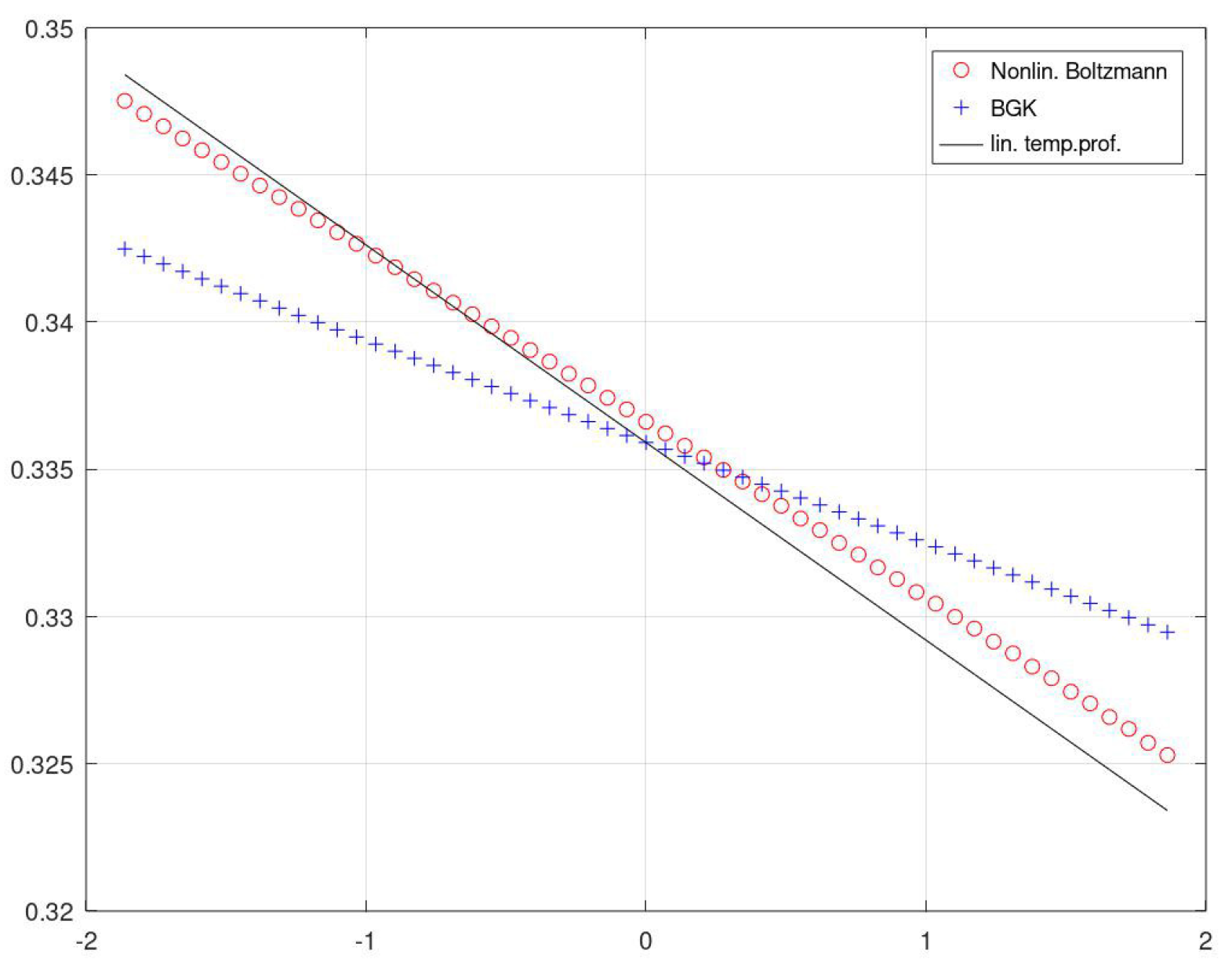
Figure 4.
Pressure closure moment for heat layer. (a) Nonlinear collision and BGK operators, (b) zoom into nonlinear operator.
Figure 4.
Pressure closure moment for heat layer. (a) Nonlinear collision and BGK operators, (b) zoom into nonlinear operator.
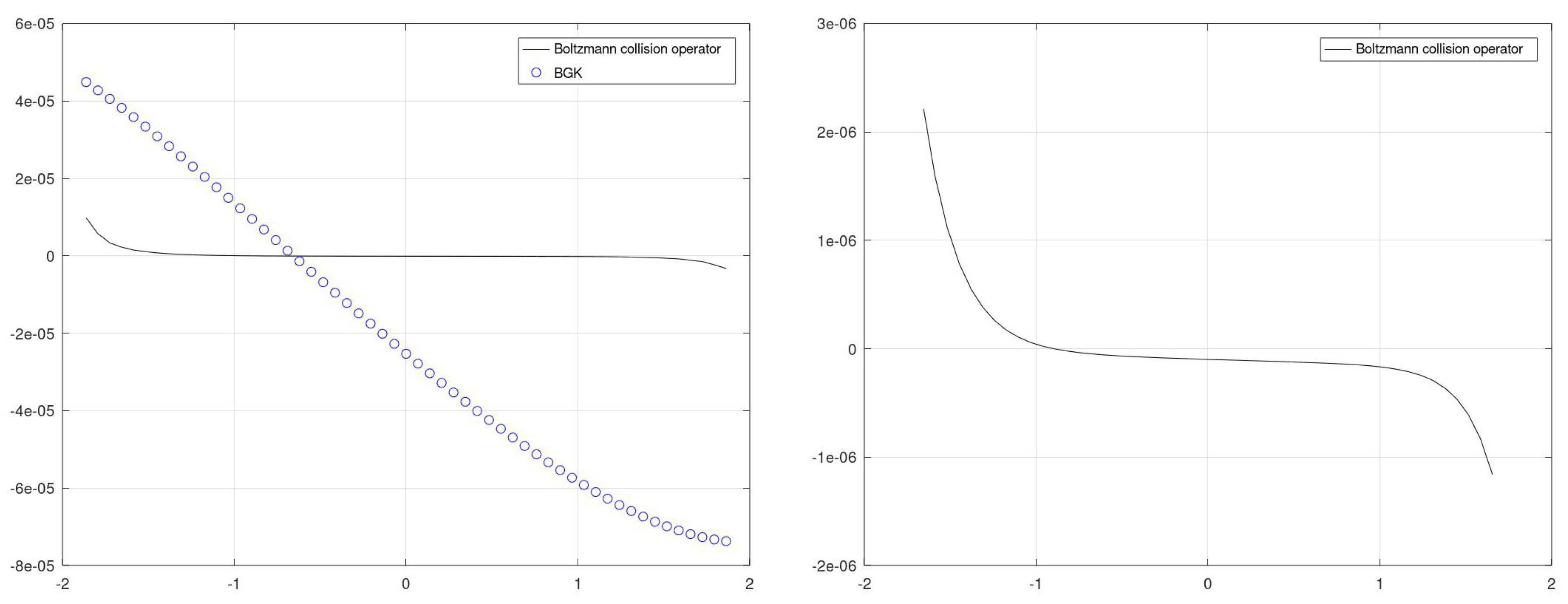
Figure 5.
Degenerate gas mixture: Boundary layer in half space .

Disclaimer/Publisher’s Note: The statements, opinions and data contained in all publications are solely those of the individual author(s) and contributor(s) and not of MDPI and/or the editor(s). MDPI and/or the editor(s) disclaim responsibility for any injury to people or property resulting from any ideas, methods, instructions or products referred to in the content. |
© 2023 by the authors. Licensee MDPI, Basel, Switzerland. This article is an open access article distributed under the terms and conditions of the Creative Commons Attribution (CC BY) license (http://creativecommons.org/licenses/by/4.0/).
Copyright: This open access article is published under a Creative Commons CC BY 4.0 license, which permit the free download, distribution, and reuse, provided that the author and preprint are cited in any reuse.


