Design of Photovoltaic System for Green Manufacturing by using Statistical Design of Experiments

1. Introduction

1.1. The Energy Policy

Energy policy is a strategy in which the government decides to address the issues of energy development along with the development of the energy industry to sustain its growth, including energy production, distribution, and consumption. The attributes of energy policy may include legislation, international treaties, and incentives to investment. It plays a vital role to mitigate the impacts of global warming and crisis of energy availability.

1.2. Importance of Solar Energy

Solar energy is one of the cleanest energy resources that does not compromise or add to global warming. The sun radiates more energy in one second than people have used since the beginning of time. Solar energy is often called “alternative energy” to fossil fuel energy sources such as oil and coal. Availability of cheap and abundant energy with minimum environmental and ecological hazards associated with its production and use is one of the important factors for desired improvement in the quality of life of the people. The growing scarcity of fossil fuels has raised global interest in the harnessing of solar energy. Solar power is a type of energy with great future potential-even though at present it covers merely a minor portion of global energy demands (0.05% of the total primary energy supply); now PV power generates less than 1% of total electricity supply. This is due to solar power still being considered the most expensive type of renewable energy. However, in remote regions of the earth it may very well constitute today's best solution for a decentralized energy supply. According to the 2010 BP Statistical Energy Survey, the world cumulative installed solar energy capacity was 22928.9 MW in 2009, a change of 46.9% compared to 2008.

1.3. Global Energy Consumption

World primary energy demand is projected in the Reference Scenario to expand by almost 60% from 2002 to 2030, an average annual increase of 1.7% per year. Demand will reach 16.5 billion tons of oil equivalents (toe) compared to 10.3 billion toes in 2002 which is shown in Table 1. On the other hand, fossil fuels will continue to dominate global energy use. They will account for around 85% of the increase in world primary demand over 2002–2030. And their share in total demand will increase slightly, from 80% in 2002 to 82% in 2030. The share of renewable energy sources will remain flat at around 4%, while that of nuclear power will drop from 7% to 5%.

Table 1. World total final consumption.

	1971	2002	2010	2030	2002–2030 (%)
Coal	617	502	516	526	0.2
Oil	1893	3041	3610	5005	1.8
Gas	604	1150	1336	1758	1.5
Electricity	377	1139	1436	2263	2.5
Heat	68	237	254	294	0.8
Biomass and waste	641	999	1101	1290	0.9
Other renewable	0	8	13	41	6.2
Total	4200	7075	8267	11, 176	1.6

Table 1. World total final consumption.

	1971	2002	2010	2030	2002–2030 (%)
Coal	617	502	516	526	0.2
Oil	1893	3041	3610	5005	1.8
Gas	604	1150	1336	1758	1.5
Electricity	377	1139	1436	2263	2.5
Heat	68	237	254	294	0.8
Biomass and waste	641	999	1101	1290	0.9
Other renewable	0	8	13	41	6.2
Total	4200	7075	8267	11, 176	1.6

Table 2. Development and installation of solar photovoltaic electricity in various countries.

Year	USA (MW)	Europe (MW)	Japan (MW)	Worldwide (MW)
2000	140	150	250	1000
2010	3000	3000	5000	14,000
2020	15,000	15,00	30,000	70,000
2030	25,000	30,000	72,000	140,000

Table 2. Development and installation of solar photovoltaic electricity in various countries.

Year	USA (MW)	Europe (MW)	Japan (MW)	Worldwide (MW)
2000	140	150	250	1000
2010	3000	3000	5000	14,000
2020	15,000	15,00	30,000	70,000
2030	25,000	30,000	72,000	140,000

1.4. Expected Future of Solar Energy Technology

Solar photovoltaic technology could harness the sun's energy to provide large-scale, domestically secure, and environmentally friendly electricity. In 2005, global solar markets reached US$ 11.8 billion, up 55% on 2004. Solar installations are expected to provide 15 GW in 2010 versus 2.7 GW in 2006. In April 2007, Photon Consulting forecast 2010 revenues from sales of solar energy equipment of US$ 90 billion, up from US$ 20 billion in 2006. Demand for silicon for solar cells is expected to increase from 41,000 tons in 2006 to 120,000 tons in 2010 and 400,000 tons in 2014. Table 2 shows the expected development and installation of solar photovoltaic electricity in the USA, Europe, Japan as well as worldwide until 2030.

Table 3. World carbon dioxide emissions by region, 1990–2025.

Region	1990	2002	2010	2015	2020	2025
Mature market economics	10,465	11,877	13,080	13,745	14,392	15,183
North America	5769	6701	7674	8204	8759	9379
Western Europe	3413	3549	3674	3761	3812	3952
Mature market Asia	1284	1627	1731	1780	1822	1852
Transitiona l economics	4894	3124	3643	3937	4151	4386
Emerging economics	6101	9408	13,478	15,602	17,480	19,222
Asia	3890	6205	9306	10,863	12,263	13,540
Middle east	845	1361	1761	1975	2163	2352
Africa	655	854	1122	1283	1415	1524
Central and south America	711	988	1289	1280	1639	1806
Total world	21,460	24,209	30,201	33,284	36,023	38,790

Table 3. World carbon dioxide emissions by region, 1990–2025.

Region	1990	2002	2010	2015	2020	2025
Mature market economics	10,465	11,877	13,080	13,745	14,392	15,183
North America	5769	6701	7674	8204	8759	9379
Western Europe	3413	3549	3674	3761	3812	3952
Mature market Asia	1284	1627	1731	1780	1822	1852
Transitiona l economics	4894	3124	3643	3937	4151	4386
Emerging economics	6101	9408	13,478	15,602	17,480	19,222
Asia	3890	6205	9306	10,863	12,263	13,540
Middle east	845	1361	1761	1975	2163	2352
Africa	655	854	1122	1283	1415	1524
Central and south America	711	988	1289	1280	1639	1806
Total world	21,460	24,209	30,201	33,284	36,023	38,790

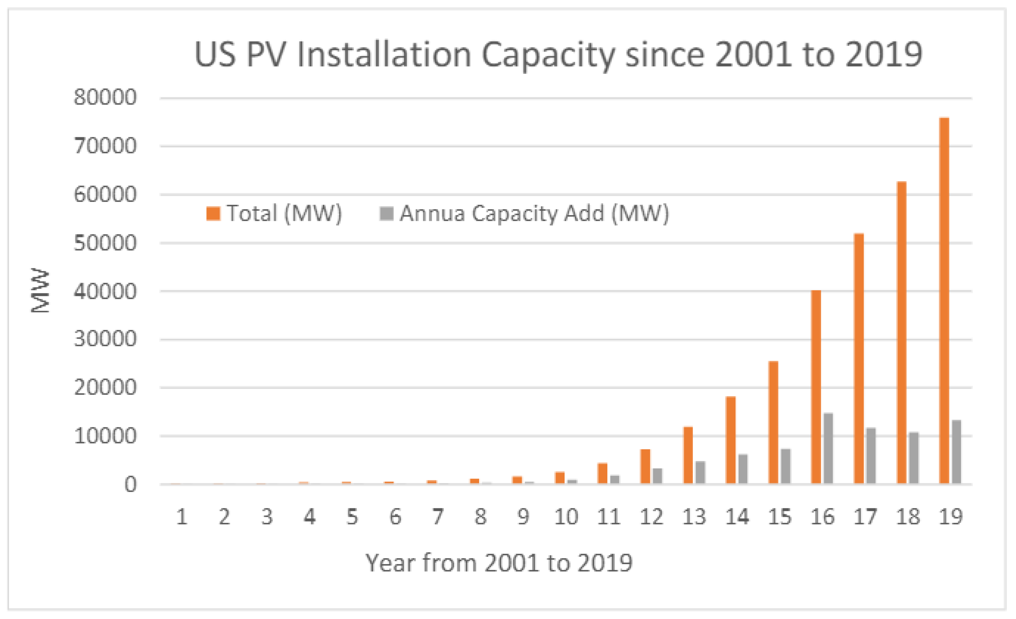
Figure 1. Solar PV Installation in the US from 2001 to 2019 (cumulative vs annual addition).

Figure 1. Solar PV Installation in the US from 2001 to 2019 (cumulative vs annual addition).

1.5. Advantage of Solar Energy

Solar energy is obviously environmentally advantageous relative to any other energy source, and the linchpin of any serious sustainable development program. It does not deplete natural resources, does not cause CO2 or other gaseous emission into air, or generates liquid or solid waste products.

• No emissions of greenhouse (mainly CO2, NOx) or toxic gasses (SO2, particulates)
• Reclamation of degraded land
• Reduction of transmission lines from electricity grids
• Improvement of quality of water resources
• Increase of regional/national energy independence.
• Diversification and security of energy supply
• Acceleration of rural electrification in developing countries

2. Methodology

The hourly wind speed data of NYC from the year 2014 to 2016 has been provided for the project. We are working for the year 2014 on this project. We have used Minitab, Excel, and Python to complete project work. For cleaning the data, we have used Python. As output, we received CSV format data and then convert the data into excel format. Data where the last number was not 51 eliminated by python software. We got 8744 hours of data and the rest 16-hour missing data we have calculated and finally, we get 8760 hours of wind speed. For statistical distribution, we have used Minitab software.

3. Result and Discussion

3.1. Question 01

For determining the mean and standard deviation, by month filter was applied and then the average and standard deviation of every month was taken. For the yearly mean and standard deviation, 8760 data were analyzed to get the values for 2014, 2015, and 2016.

Mean speed for 2015 = 4.875 m/s

Mean speed for 2014 = 5.07 m/s

Mean speed for 2016 = 5.15 m/s

Standard Deviation for 2015 = 2.6585

Standard Deviation for 2014 = 2.73

Standard Deviation for 2016 = 2.79

For the yearly mean and standard deviation for the year 2014, the rand () function in Excel was used to create a random sample and then 1000 data points were collected from that group. From the 1000 random data points, the month wise mean and standard deviation for 2014 was calculated and they are as follows:

Month	Mean (M/S)	Standard Deviation
January	6.09	2.93
February	5.93	3.27
March	5.29	2.86
April	5.36	2.84
May	4.41	2.75
June	4.56	2.2
July	4.18	2.09
August	4.27	2.09
September	4.10	2.09
October	5.22	2.34
November	4.49	2.52
December	5.49	1.54

3.2. Question 02

Figure 2. Probability plot of wind speed with normal distribution.

Figure 2. Probability plot of wind speed with normal distribution.

Figure 3. Probability plot of wind speed with exponential distribution.

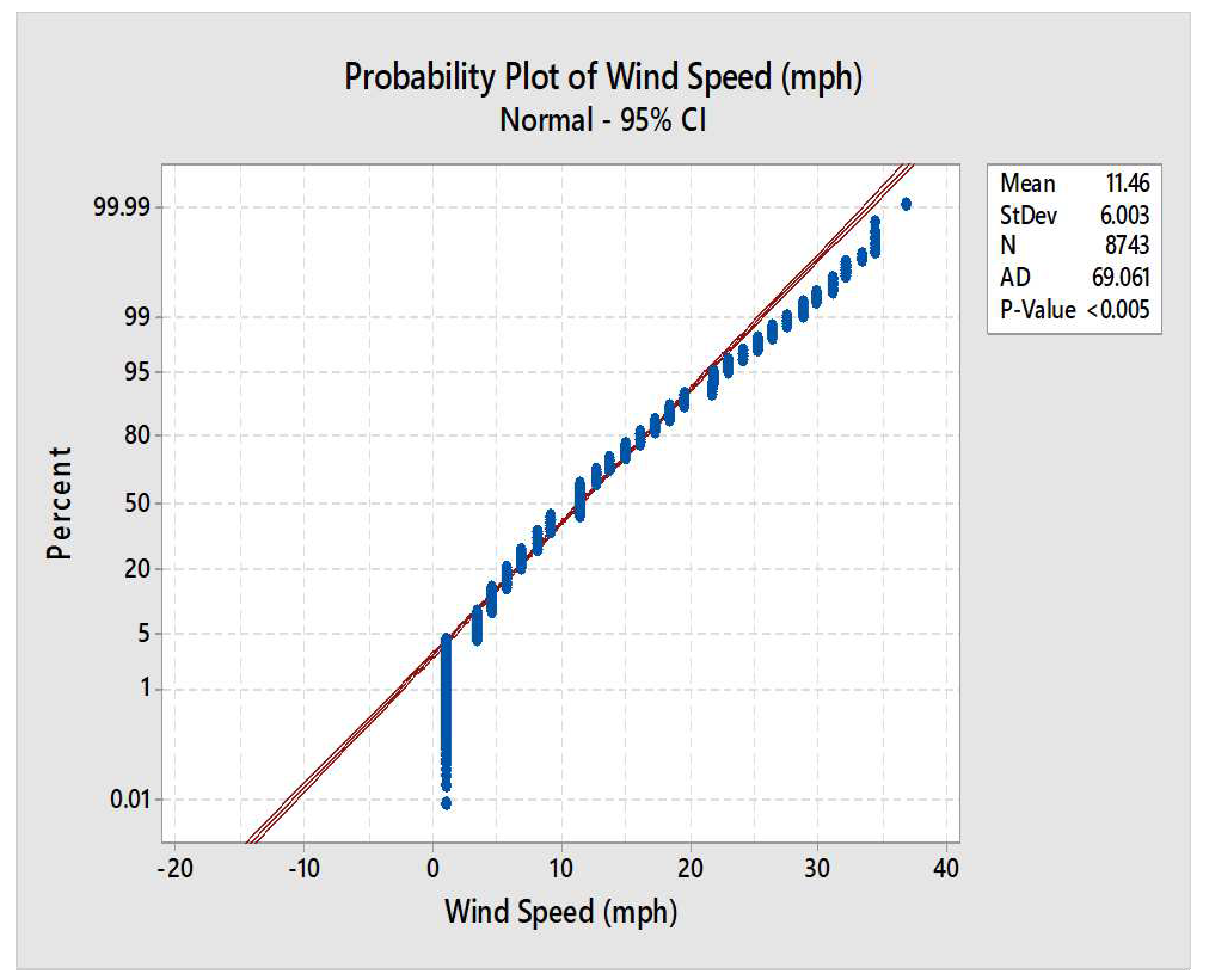
Figure 3. Probability plot of wind speed with exponential distribution.

Figure 4. Probability plot of wind speed with lognormal distribution.

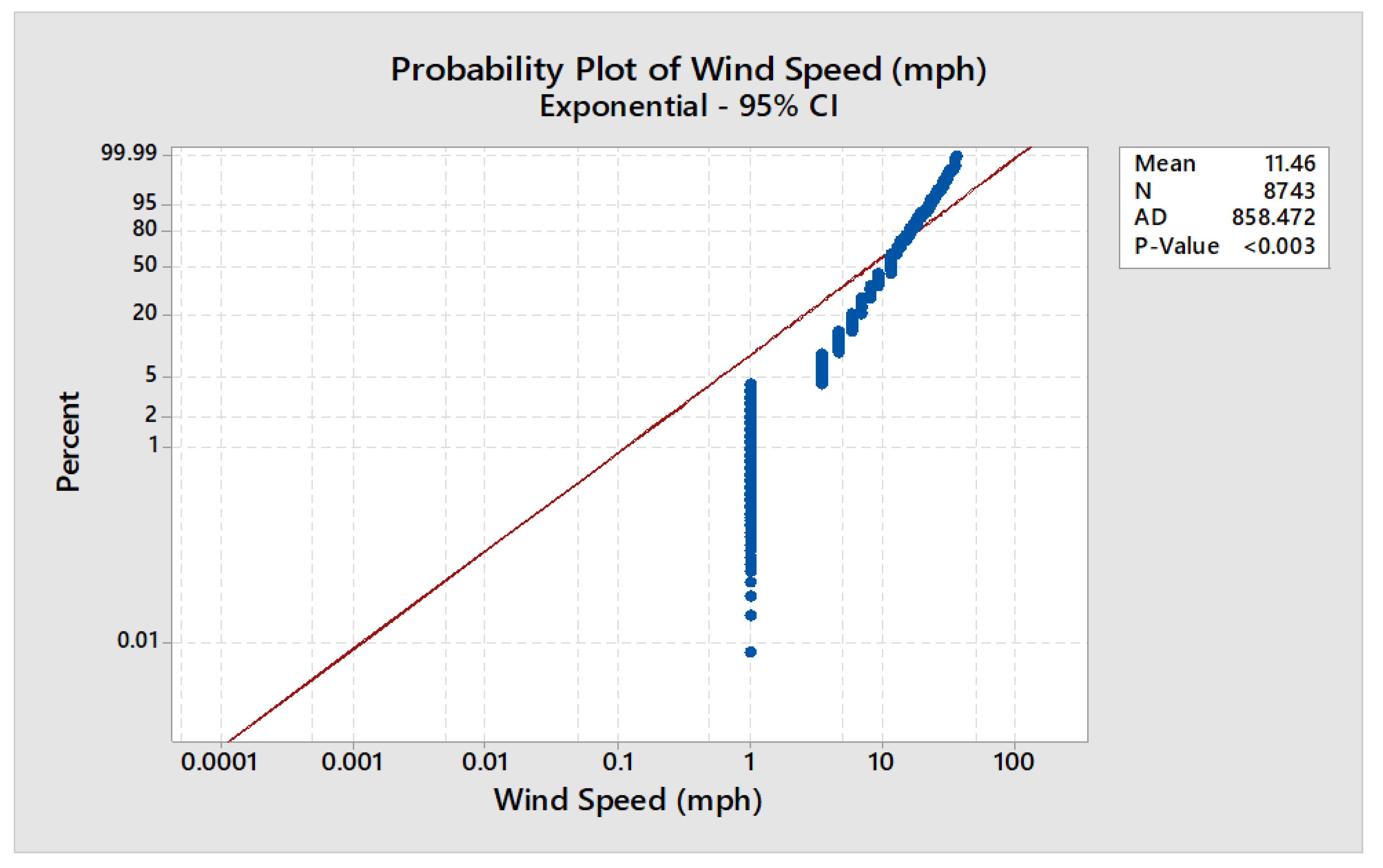
Figure 4. Probability plot of wind speed with lognormal distribution.

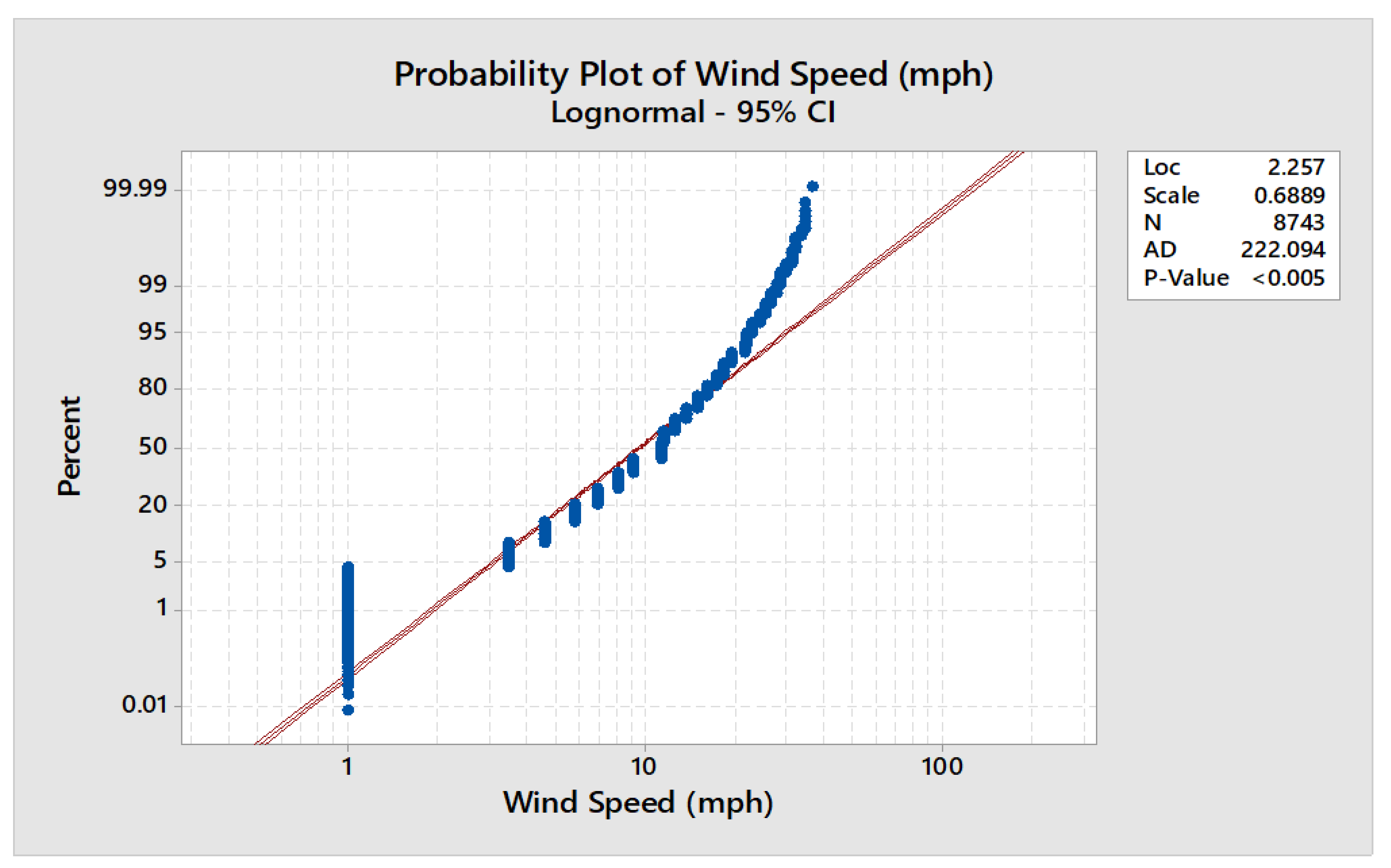
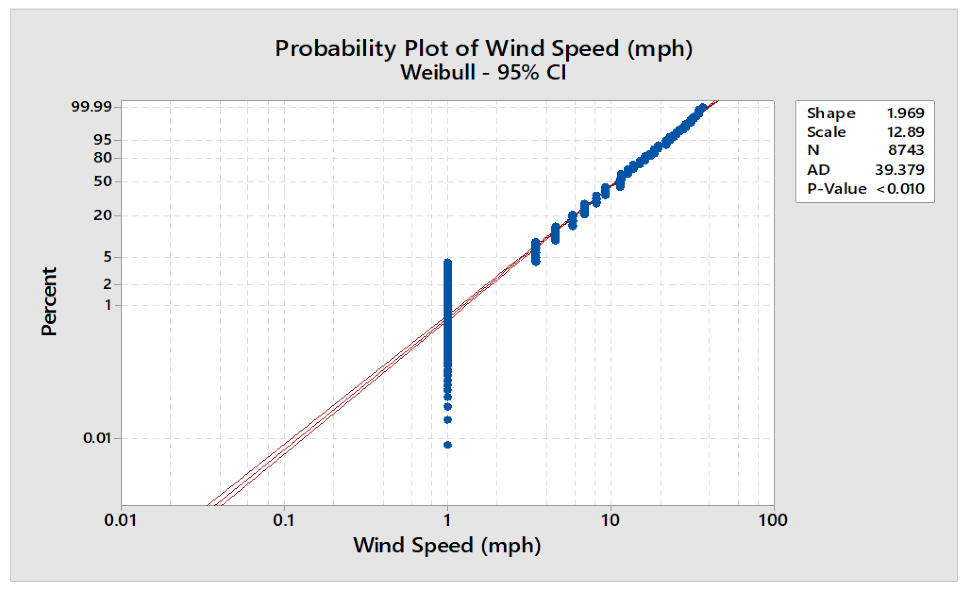
Using Minitab to fit a random sample of 1000, we concluded that the Weibull distribution is the best fit but still has a low p-value of <0.01. The second-best distributions were normal distribution with a p-value <0.005.

Figure 5. Probability plot of wind speed with Weibull distribution.

Figure 5. Probability plot of wind speed with Weibull distribution.

3.3. Question 03

✓

Hypothesis testing on windspeed means, Null Hypothesis: Ho: uo = u1

✓

Alternative hypothesis: H1: uo≠u1

✓

The mean of the 1000 random value of wind speed of 2015 is = 4.85 m/s

✓

The variance of the 1000 random value of wind of 2015 speed is = 7.05

✓

Standard deviation = 2.64

✓

The mean of the 1000 random value of wind speed of 2016 is = 5.05m/s

✓

The variance of the 1000 random value of wind of 2016 speed is = 7.78 m/s

✓

Standard deviation = 2.78 m/s

✓

Sp= 2.72

✓

to = -0.51

✓

to falls in between the range. Hence, we fail to reject the null hypothesis. So, the mean wind speed is not significantly different between two adjacent years.

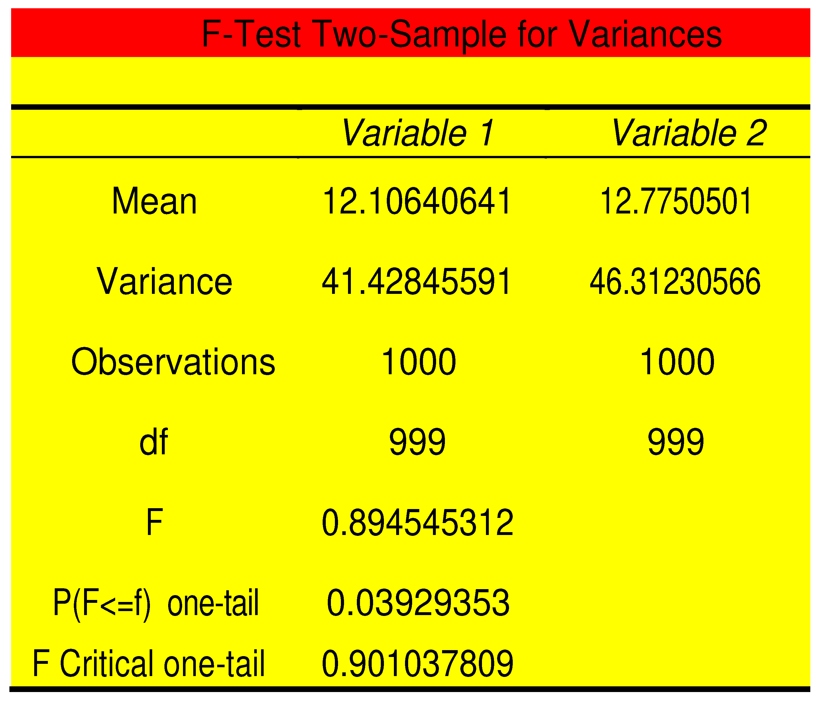
Here, F value is less than the F critical value, so we fail to reject the null hypothesis using 95% confidence level.

Figure 6. F-test of two samples for variances.

Figure 6. F-test of two samples for variances.

3.4. Question 04

We have taken 1000 sample data from the 8760 data to estimate the yearly wind speed. We have used Vh = Vg (80/8)³ to find the wind speed at turbine height. We have also removed the data which are unable to operate wind turbine. So, we have eliminated the wind speed less than 2m/s and greater than 25m/s. This gives us 330 data where wind turbine can operate between wind speed 12 m/s to 25 m/s.

The output will be = 2 MW/h*330 hrs. = 650 MWh. Between 0 to 2m/s numbers of samples = 32 Between 2 to 4m/s numbers of samples = 106 Between 4 to 6m/s numbers of samples = 134 Between 6 to 8m/s numbers of samples = 196 Between 8 to 10m/s numbers of samples = 150 Between 10 to 12m/s numbers of samples = 52

Wind Speed (m/s)	12-25	10-12	8-10	6-8	4-6	2-4
Power (MW)	2	1.75	1.5	1.25	0.75	0.25

From 1000 random data we have calculated total power =

(330Hrs x 2MWh) + (52Hrs x 1.75MWh) + (150Hrs x 1.5MWh) + (196Hrs x 1.25MWh) +

(134Hrs x .75MWh) + (106Hrs x .25MWh) = 1348 MWh total

For total 8760 data it will be = (1348/1000) *8760 = 11,808.48 MWh total

So, the number of homes wind turbine could power = (11,808.48*1000)/7300 = 1618 homes

3.5. Question 05

Figure 7. Sample calculation for question 5.

Figure 7. Sample calculation for question 5.

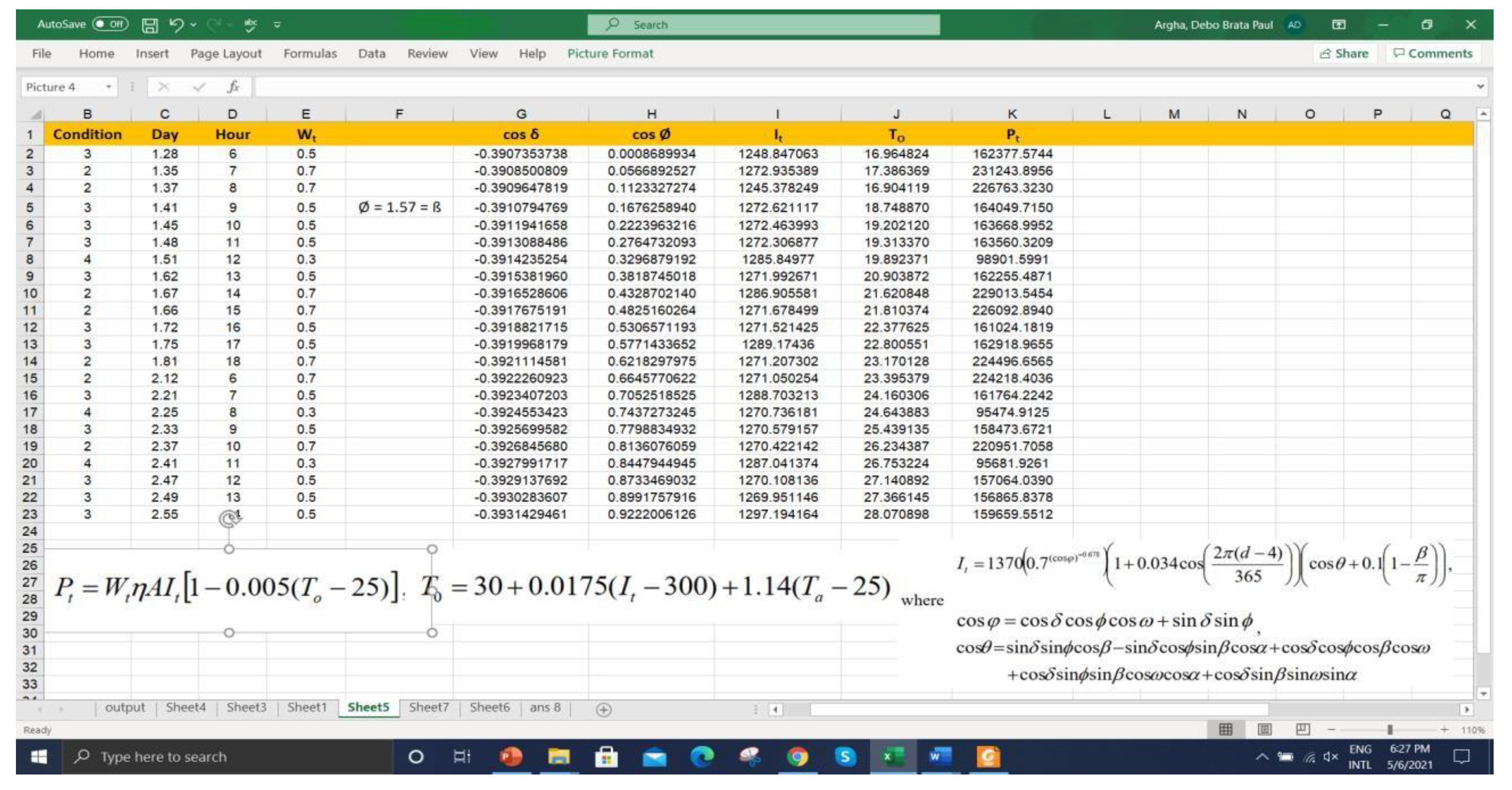
For PV output all-night data have been deleted and set the PV angle to the same as the latitude of NYC to maximize output. After calculating the sunrise and sunset time, excel was used to find solar irradiance at every hour. To find the power output I mapped the given data condition range of 1-9 to the required 1-0. Then the power output at every hour could be established for the panels. After power output at every hour was found the sum has been calculated and found the yearly power output.

In total, the solar panels generated 867.37 MWh.

3.6. Question 06

Figure 8. Hourly wind speed forecasting for January 02, 2014.

Figure 8. Hourly wind speed forecasting for January 02, 2014.

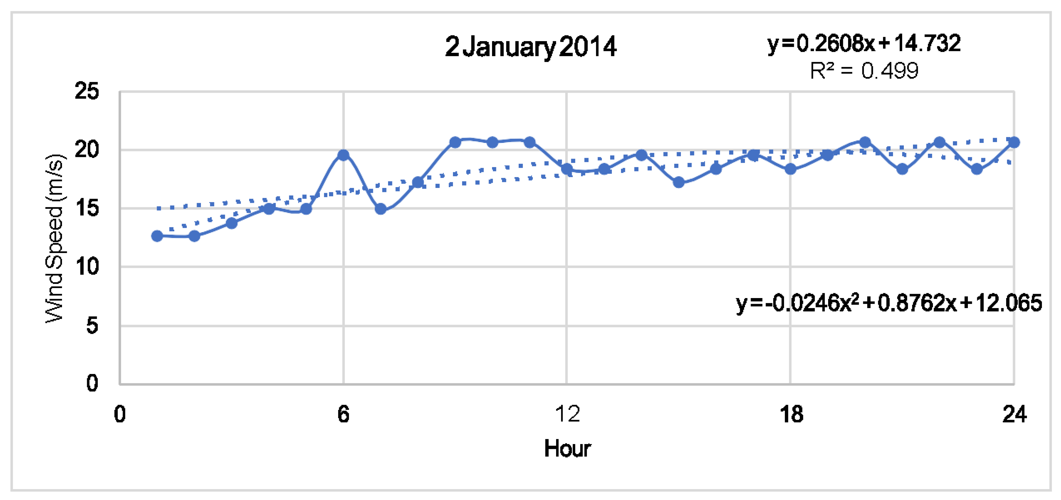
Using the second order of polynomial line, the equation for forecasting is:

y = -0.0246x² + 0.8762x + 12.065

For the linear fit model, equation is, y = 0.2608x + 14.732.

Figure 9. Monthly wind speed forecasting for January 2014.

Figure 9. Monthly wind speed forecasting for January 2014.

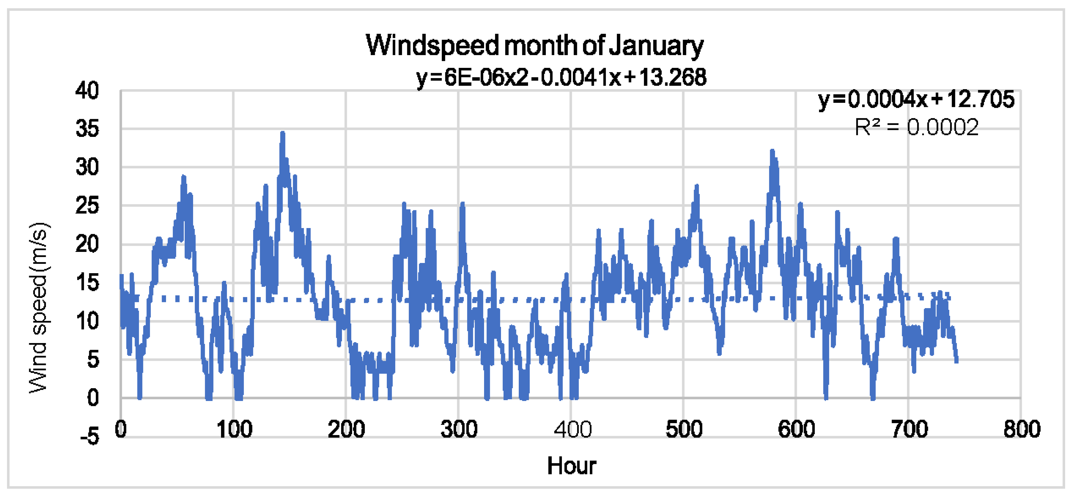
For monthly wind speed estimation, we averaged the daily windspeed for January 2014, using this data then plotted the daily windspeed average vs the day of the month. For a second-order polynomial trend line, the equation obtained is, y = 6E-06x² - 0.0041x + 13.268

A linear trend line gives the equation: y = 0.0004x + 12.705.

Figure 10. Yearly wind speed forecasting for January 2014.

Figure 10. Yearly wind speed forecasting for January 2014.

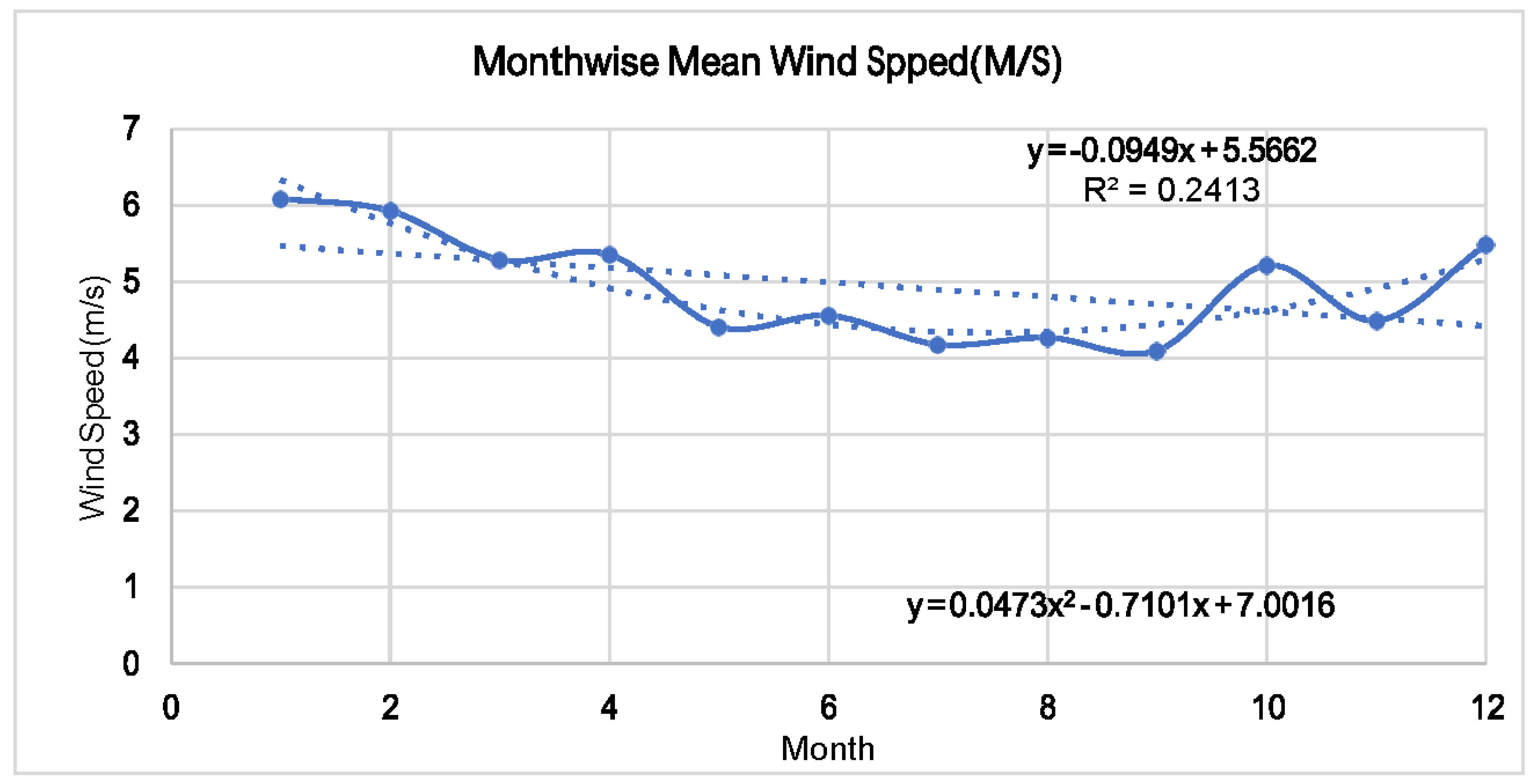
For yearly wind speed, the average wind speed for every month for the year 2014 was calculated and plotted vs the number of the month. The formula for the second-degree polynomial is y = 0.0473x² - 0.7101x + 7.0016

Using a Linear line of fit we got, y = -0.0949x + 5.5662.

3.7. Question 07

Factors that are significant and/or correlated:

Factor 1. The Size of PV system: The size of the PV is one of the important factors. The energy generation will increase with the PV size.

Factor 2. PV Capacity Cost: The cost is the most important factor that can be calculated by the multiplication of the number of PV panels and the installation cost. The equation is 106x. Here, x

= PV size in MW.

Factor 3. PV Efficiency: The PV efficiency has been selected as maximum as 25%. If we don’t care much about cost, the efficiency can be increased in a limited size.

Factor 4. Weather Condition: In perfect weather conditions, the factory needs 100,000 m2 panels to handle roughly 27 MW assuming each panel generates 270 W/m2. The angle of the sun and weather conditions have a great effect on the fluctuation of power, on average in NYC is 130 W/m2.

In January 2014 average weather condition in New York is 0.412 representing the solar cells generate about 41% of their maximum output during the day in winter. Whereas in summer the value is 0.453 or 45% of maximum generation

Factor 5 and 6. Ambient Temperature and Wind Speed: Ambient temperature and wind speed have also an effect on panel efficiency. Both are helping to cool down the PV systems, making them run more efficiently.

Factor 7. Hour of a Day: The power can be generated in daytime, not at night and the maximum power can be found at noon. Based on the formula, in January (winter) it is 1274.76 W/m2 and in summer it is 1468.6 W/m2.

Factor 8 & 9. Utility Pricing Scheme and Government Incentives: Utility scheme could offer an income possibility if the PV system is generating more power than it is consuming, and Government incentives could drastically lower the upfront price of panel installation.

Factor 10. The batter capacity: battery capacity can reduce the size of the PV system by storing energy when power generation is over the factory power usage and discharging it during bad weather or at night.

In winter, the factory has a peak energy draw of 17.4 MW during hours 13 and 16. So the expected power generation in January 1274.76 W × 25% × 1m2 × 0.412 × 1.0309 (from temperature) = 135.4.

In summer, 1468.6 W × 25% × 1m2 × 0.453 × 0.8621 = 143.4.

In winter, factory draws an average of 14.78 MW with a peak of 17.4 MW. Minimum we need

17.4 × 106/ 135.4 = 128,509 panels at 1 m2 each. In summer, minimum we need 22.6 × 106/143.4

= 157,602 panels at 1 m2 each.

If the panels make an average of 17.4 MW during the daytime (from hour 7 to 17), we can create

17.4 × 10 = 174 MWh per day. The factory needs 14.78 × 24 = 354.8 MWh. So, the system would need an average of 35.48 MW/hour for 10 hours to generate enough energy for daytime power draw peaks and night usage.

If we use a 60 MW system, simulation gives us average excess energy storage of 62.3 MW/day.

If a 510 MW battery is installed, it would take 510/62.3 = 8.2 day to fully charge and can be capable of providing a little over one day of full power outage.

3.8. Question 08

Life cycle cost analysis

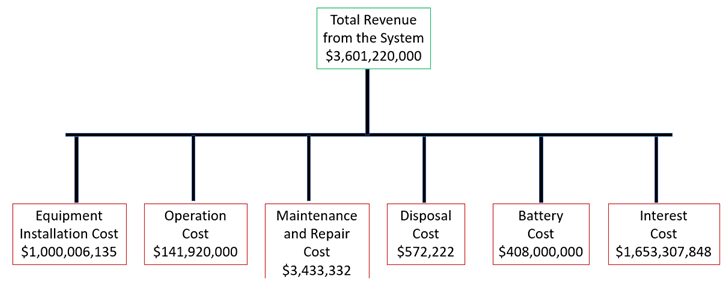
Cost of Electricity by source in US

Power Plant Type	Cost (LCOE)
	$/kW-hr
Coal with CCS	$0.12-0.13
CC Natural Gas	$0.04
CC with CCS	$0.08
Nuclear	$0.09
Wind onshore	$0.04
Wind offshore	$0.11
Solar PV	$0.04
Solar Thermal	$0.17
Geothermal	$0.04
Biomass	$0.09
Hydro	$0.03

(Levelized cost of electricity, LCOE) Source: Adapted from US DOE

4. Conclusion

Solar power is an immense source of directly useable energy and ultimately creates other energy resources: biomass, wind, hydropower, and wave energy. Most of the Earth's surface receives sufficient solar energy to permit low-grade heating of water and buildings, although there are large variations with latitude and season. At low latitudes, simple mirror devices can concentrate solar energy sufficiently for cooking and even for driving steam turbines. The energy of light shifts electrons in some semiconducting materials. This photovoltaic effect is capable of large-scale electricity generation. However, the present low efficiency of solar PV cells demands very large areas to supply electricity demands. Direct use of solar energy is the only renewable means capable of ultimately supplanting the current global energy supply from non-renewable sources. It is cheaper compared to all other sources of source. In the coming days production will be less and solar energy will be more feasible comparative to the present days.

References

- Cesare, S. Survey of Energy Resources 2015––Solar Energy; World Energy Council: London, UK, 2015. [Google Scholar]
- A review on energy saving strategies in industrial sector. Renew. Sustain. Energy Rev. 2011, 15, 150–168. [CrossRef]
- The 2010 PVPS Annual Report shows that exports comprised around 95% of China’s production from 2006 to 2010. PVPS Annual Report 2010, April 14, 2011, p. 51. Available online: http://www.iea-pvps.org/index.php?id=6.
- For a comparison of green energy programs and policies in China and the United States, see CRS Report R41748, China and the United States—A Comparison of Green Energy Programs and Policies, by Richard J. Campbell.
- Available online: https://en.wikipedia.org/wiki/Cost_of_electricity_by_source.
- U.S. Solar Photovoltaic Manufacturing: Industry Trends, Global Competition, Federal Support, Michaela D. Platzer, Specialist in Industrial Organization and Business, 30 May 2015.
- Mekhilef, Saidurb, Safaria, A review on solar energy use in industries-2014.
Disclaimer/Publisher’s Note: The statements, opinions and data contained in all publications are solely those of the individual author(s) and contributor(s) and not of MDPI and/or the editor(s). MDPI and/or the editor(s) disclaim responsibility for any injury to people or property resulting from any ideas, methods, instructions or products referred to in the content. |
© 2023 by the authors. Licensee MDPI, Basel, Switzerland. This article is an open access article distributed under the terms and conditions of the Creative Commons Attribution (CC BY) license (http://creativecommons.org/licenses/by/4.0/).
Copyright: This open access article is published under a Creative Commons CC BY 4.0 license, which permit the free download, distribution, and reuse, provided that the author and preprint are cited in any reuse.