Dynamics of the Static Star Differential System from the Mathematical and Physical Point of Views

Preprint

Article

Dynamics of the Static Star Differential System from the Mathematical and Physical Point of Views

Altmetrics

Downloads

114

Views

Comments

Joan C. Artés,

Jaume Llibre^*,Nicolae Vulpe

Joan C. Artés,

Jaume Llibre^*,Nicolae Vulpe

This version is not peer-reviewed

Submitted:

23 October 2023

Posted:

24 October 2023

You are already at the latest version

Alerts

Abstract

We classify all the topologically non-equivalent phase portraits of the quadratic polynomial differential system dx/dt = (1-2x)(y-x), dy/dt =y (2-g y-(5g-4)x/(g-1)), in the Poincaré disc for all the values of the parameter g in R\{1}. The differential system dx/dt = y-x, dy/dt =y (2-g y-(5g-4)x/(g-1))/(1-2x), when the parameter g in (1,2] models the structure equations of a static star in general relativity in the case of the existence of a homologous family of solutions, being x = m(r)/r where m(r)>= 0 is the mass inside the sphere of radius r of the star, y = 4pi r^2 rho where rho is the density of the star, and t = ln (r/R) where R is the radius of the star. We classify the possible values of m(r)/r and 4pi r^2 rho when r-->0.

Keywords:

Subject: Physical Sciences - Mathematical Physics

MSC: 34C05

1. Introduction and the Main Results

The structure equations of a static star in general relativity in the case of the existence of a homologous family of solutions are

\begin{matrix} \dot{x} = y - x, \\ \dot{y} = \frac{y}{1 - 2 x} (2 - γ y - \frac{5 γ - 4}{γ - 1} x), \end{matrix}

(1)

where the parameter

γ

varies in the interval

(1, 2]

, and the dot denotes derivative with respect to the variable

t = ln (r / R)

being R the radius of the star. Therefore, from the physical point of view we are interested in the solutions defined in the interval

t \in (- \infty, 0)

. Here

x = m (r) / r

where

m (r) \geq 0

is the mass inside the sphere of radius r of the star,

y = 4 π r^{2} ρ

being

ρ

the density of the star. For more details on the differential system (4) see [3,4,5,7,8,10].

We remark that from the physical point of view and since

x > 0

and

y > 0

we are mainly interested in the dynamics of the differential system (4) with

γ \in (1, 2]

in the set

Q^{*}

formed by the positive quadrant

Q = {(x, y) \in R^{2} : x > 0, y > 0}

R^{2}

without the straight line

x = 1 / 2

where the differential system (4) is not defined.

Note that the straight line

y = 0

is invariant because when

y = 0

we have that

\dot{y} = 0

. Therefore, since

\dot{x} |_{x = 0} = y

the set

Q^{*}

is positively invariant, i.e. orbits of system (4) can enter in

Q^{*}

through the positive y-axis but never orbits of the quadrant Q can exit from

Q^{*}

Doing the change of the independent variable

t \to s

, where

d t = (1 - 2 x) d s

the differential system (4) becomes the polynomial differential system

\begin{matrix} \dot{x} = (1 - 2 x) (y - x) = p (x, y), \\ \dot{y} = y (2 - γ y - \frac{5 γ - 4}{γ - 1} x) = q (x, y), \end{matrix}

(2)

where now the dot denotes derivative with respect to the variable s.

The differential system (2) is a polynomial differential system of degree 2 because the maximum of the degrees of the polynomials

p (x, y)

and

q (x, y)

is 2. The polynomial differential systems of degree 2 are called simply quadratic systems and they have been intensively studied, see for instance the books [1,11,13], the paper [5], and the hundreds of references quoted therein.

The domain of definition of the differential system (2) is the whole plane

R^{2}

. The decomposition of

R^{2}

as union of the orbits of system (2) is the phase portrait of the differential system (2). In particular a phase portrait shows where each orbit is born and where each orbit dies, if they are equilibrium points, periodic orbits, ... In summary a phase portrait provides all the qualitative information about the orbits of a differential system. For more information about the phase portraits of the planar differential systems see for instance [6].

The phase portraits of the polynomial differential systems in

R^{2}

are usually described in the Poincaré disc. Roughly speaking the Poincaré disc is the unit closed disc

D^{2}

whose interior has been identified with the plane

R^{2}

and whose boundary, the circle

S^{1}

is identified with the infinity of

R^{2}

. Note that in the plane

R^{2}

we can go to infinity in as many directions as points has the circle

S^{1}

. For more details on the Poincaré disc see Chapter 5 of [6] or the Appendix.

As usual two phase portraits in the Poincaré disc

D^{2}

are topologically equivalent if there is a homeomorphism of

D^{2}

which sends orbits of the first phase portrait into orbits of the second phase portrait preserving or reversing the sense of all the orbits.

The objective of this paper is double. First we study the phase portraits of the quadratic systems (2) from a mathematical point of view, i.e. for all the values of parameter

γ \in R ∖ {1}

where the system is defined. These phase portraits are described in the Poincaré disc, in this way we control the orbits which escape or come from the infinity. Second we describe the whole dynamics of the static star in general relativity in the case of the existence of a homologous family of solutions modelled by the differential system (4) for

1 < γ \leq 2

in the positive quadrant taking into account the orbits which could escape or come from the infinity.

Our main results are described in the next two theorems.

Theorem 1.

The quadratic system (4) when γ varies in

R ∖ {1}

has 11 topologically non-equivalent phase portraits in the Poincaré disc. These are the phase portraits

γ_{1}

γ_{2}

γ_{3}

γ_{4}

γ_{5}

γ_{8}

γ_{9}

γ_{12}

γ_{13}

γ_{15}

and

γ_{16}

given in Figure 1.

Theorem 1 is proved in Section 2.

In Figure 1 appear other few phase portraits which are needed to complete the bifurcation diagram as it is described in the proof of Theorem 1.

We define

Q_{1} = Q^{*} \cap {x < 1 / 2}

and

Q_{2} = Q^{*} \cap {x > 1 / 2}

Theorem 2.

The static star in general relativity in the case of the existence of a homologous family of solutions modelled by the differential system (4) with

1 < γ \leq 2

verifies the following statements.

(a): The region $Q_{1}$ is positively invariant, and the region $Q_{2}$ is invariant, i.e if an orbit of the system has a point in $Q_{2}$ the whole orbit is contained in $Q_{2}$ .
(b): The orbits in $Q_{2}$ when $r \to 0$ verify that $4 π r^{3} ρ \to 0$ and $m (r) / r \to \infty$ .
(c): If

$\frac{m (R)}{R} = 4 π R^{2} ρ = - \frac{2 (γ - 1)}{γ^{2} + 4 γ - 4},$

then

$\frac{m (r)}{r} = 4 π r^{2} ρ = - \frac{2 (γ - 1)}{γ^{2} + 4 γ - 4},$

for all $r \in (0, R]$ .
(d): For every initial condition $(\frac{m (R)}{R}, 4 π R^{2} ρ)$ in $Q_{1}$ distinct from

$(- \frac{2 (γ - 1)}{γ^{2} + 4 γ - 4}, - \frac{2 (γ - 1)}{γ^{2} + 4 γ - 4}),$

the orbit determined for this condition when r tends to some finite value $r_{0} < R$ (which depends on the initial condition) satisfies

$\frac{m (r)}{r} \to 0 a n d 4 π r^{2} ρ \to k \geq 0,$

where k can take any non-negative value when the initial condition varies.

Theorem 2 is proved in Section 3.

The techniques used for studying this 2-dimensional polynomial differential system, can be extended to higher dimensions, see for instance [9].

2. Proof of Theorem 1

Even the study of the bifurcation diagram of this system is not complicate because it has just one parameter, we will make use of the Theory of Invariants developed by the Sibirskii school, and fully developed for quadratic systems in the book [1]. The invariants (and also the comitants) allow to easily determine all the geometric features provided by the system in a methodic and consistent way. These geometric features may even exceed the most simple topological features to which later we will reduce the classification.

Each one of these geometric features is characterized using some of the following 10 invariant polynomials:

\{μ_{0}, μ_{1}, μ_{2}, μ_{3}, μ_{4}, D, W_{4}, B_{1}, B_{2}, B_{3}, η\} .

(3)

The invariants

B_{1}

B_{3}

can be found in page 14 of [12]. The rest of invariants can be found in pages 121-128 of [1].

Apart from the geometric properties of the singularities, there may also exist bifurcations due to separatrix connections. If these connections are invariant straight lines or polynomial curves, they may also be determined by means of algebraic invariants. But they may also be of non-algebraic nature in which case, only an analytical and numerical study may detect them. Anyway we will not meet any of them in this family.

The first important detail to be remarked of this system is that it is not defined for

γ = 1

. Thus the bifurcation diagram will show a jump from cases with

γ < 1

to cases with

γ > 1

and no continuity or coherence must be expected from ones to the others.

Next we detect that for every

γ

the straight lines

y = 0

and

x = 1 / 2

are invariant. For some values of

γ

we may have more invariant straight lines. It is a known result that quadratic systems having two invariant lines cannot have limit cycles (see [2]), so systems (2) has no limit cycles.

The first relevant invariant is

μ_{0} = \frac{4 γ (γ^{2} + 4 γ - 4)}{γ - 1}

which if it vanishes (for some

γ

), will determine if a finite singularity escapes to infinity. For one of the possible solution of

μ_{0} = 0

we will have that

μ_{1} = μ_{2} = μ_{3} = μ_{4} = 0

implying then that the system has an infinite number of finite singularities, see Lemma 5.2 (iii) in [1] .

One usual generic invariant is

D

which determines (when it vanishes) that two finite singularities have collided, but for these systems

D = - \frac{192 γ^{6}}{{(γ - 1)}^{4}}

and

γ = 0

is exactly the value mentioned above for which the systems degenerate. By degenerate system we mean that there is an infinite number of finite singular points (real or complex), which is equivalent to say that the two equations defining the differential system have a non constant common factor.

We will also need the invariant

η = \frac{{(γ - 2)}^{2} {(7 γ - 6)}^{2}}{{(γ - 1)}^{2}}

which if equal to zero, determines if two infinite singularities coalesce.

Another interesting geometric feature to capture is whether the system has or not invariant straight lines. Sometimes these lines will not imply a separatrix connection and thus, breaking them will not produce a different phase portrait. However, other times, on these lines we will find separatrix connections and they must be included in the bifurcation diagram. The invariants/comitants that will help us to find those invariant straight lines are

B_{1}

B_{2}

and

B_{3}

. Since

B_{1} = B_{2} = 0

for this family we must just concentrate on

B_{3}

which is

B_{3} = - \frac{3 γ {(3 γ - 2)}^{2} x^{2} y^{2}}{{(γ - 1)}^{2}} .

We normally add one more invariant in every study which is

W_{4}

. This invariant detects the transition from a node to a strong focus when the invariant changes its sign. This does not produces a topological change in the phase portrait. Since the fact that an antisaddle is a node or a focus may have some physical interest, we have preferred to include it.

In summary, extracting from the different invariant/comitants the equations that must be solved for obtaining the mentioned qualitative informations are

\begin{matrix} γ (γ^{2} + 4 γ - 4) = & 0, \\ {(γ - 2)}^{2} {(7 γ - 6)}^{2} = & 0, \\ γ {(3 γ - 2)}^{2} = & 0 . \end{matrix}

(4)

Then easy computations determine that the bifurcations points are the values

\begin{matrix} γ_{2} = - 2 (1 + \sqrt{2}), & γ_{4} = 0, & γ_{6} = 2 / 3, \\ γ_{8} = 2 (\sqrt{2} - 1), & γ_{12} = 6 / 7, & γ_{14} = 1, \\ γ_{16} = 2 . \end{matrix}

(5)

We have numerated them with even numbers and leaving some gaps in order to leave space for intermediate generic cases and the values where

W_{4} = 0

. We have also assigned a place for the case

γ = 1

even knowing that the differential system is undefined there so to maintain the coherence in the numeration between generic cases (odd) and singular (even).

The invariant

W_{4} = \frac{9 γ^{6} {(3 γ - 2)}^{2} (γ^{2} - 44 γ + 36)}{{(γ - 1)}^{6}}

only changes sign on the roots of the non multiple component of degree 2. We must solve it. And now we add intermediate values between each singular values. So in order to obtain all the bifurcation diagram of the differential system (2) we must study it for the following values of the parameters:

\begin{matrix} γ_{1} = - 5, & γ_{2} = - 2 (1 + \sqrt{2}), & γ_{3} = - 2, \\ γ_{4} = 0, & γ_{5} = 1 / 3, & γ_{6} = 2 / 3, \\ γ_{7} = 7 / 10, & γ_{8} = 2 (\sqrt{2} - 1), & γ_{9} = 83 / 100, \\ γ_{10} = 2 (11 - 4 \sqrt{7}), & γ_{11} = 84 / 100, & γ_{12} = 6 / 7, \\ γ_{13} = 88 / 100, & γ_{14} = 1, & γ_{15} = 3 / 2, \\ γ_{16} = 2, & γ_{17} = 4, & γ_{18} = 2 (11 + 4 \sqrt{7}), \\ γ_{19} = 50 . \end{matrix}

(6)

Now using the program P4 (see [6]) we obtain a picture of every phase portrait and we describe briefly the bifurcations, explaining what has happened when we move from a case to another one. In fact we additionally have verified that all the local phase portraits of the finite and infinite equilibrium points of the differential system (4) are the ones obtained by the program P4. Thus the local phase portraits of the hyperbolic equilibrium points (i.e. the ones such that the eigenvalues of the linear part of the system evaluated on them have real part non-zero) have been computed with Theorem 2.15 of [6]. The local phase portraits of the semi-hyperbolic or also called semi-elemental equilibrium points (i.e. the ones such that one and only one of the eigenvalues of the linear part of the system evaluated on them is zero) have been computed with Theorem 2.19 of [6]. The local phase portraits of the nilpotent equilibrium points (i.e. the ones such that both eigenvalues of the linear part of the system evaluated on them are zero but the linear part is not identically zero) have been computed with Theorem 3.5 of [6].

Once we now all the local phase portraits of the finite and infinite equilibrium points in order to determine the global phase portraits in the Poincaré disc for the different values of the parameter

γ

we only need to control where start and end the separatrices of the differential system. For the differential systems (4) the separatrices are all the orbits of the infinity, the finite equilibrium points and the separatrices of the hyperbolic sectors of the finite and infinite equilibrium points, for more details see section 1.9 of [6]. The limit cycles, when they exist, also are separatrices but the differential systems (4) has no separatrices for the reason previously explained.

For

γ_{1}

we see two saddles on the x-axis and a finite node. The infinite singularity

N_{1} = [1 : 0 : 0]

is an elemental node. There is another infinite singularity at

N_{2} = [0 : 1 : 0]

which is also an elemental node. On these two singularities we have the ends of the finite invariant straight lines. And there is a third equilibrium point at infinity (on first and third quadrant)

N_{3}

which is an elemental saddle. The phase portrait is completely determined by the invariant straight line and the distribution of singularities. We draw in wide solid black the separatrices and in thin black the orbits. The parts of the invariant straight lines which are not separatrices, we draw with dashes.

For

γ_{2}

we see that the finite node in the third quadrant has coalesced with the infinite singularity

N_{3}

producing a semi-elemental saddle-node

\bar{(\binom{1}{1})} S N

(see notation in Section 3.7 or Appendix A of [1]).

For

γ_{3}

the infinite singularity

N_{3}

ejects a saddle into the first quadrant and remains as a node.

γ_{4}

the system degenerates. The invariant straight line

x = 1 / 2

becomes fulfilled with singularities. While other bifurcations normally need simply the change of one property of the system, this type of bifurcation usually implies several important changes and the next phase portrait needs to be completely described.

γ_{5}

the saddle that we had before on the intersection of the two invariant straight lines, now reappears as a node. And the infinite singularity

N_{2}

which was before a node, now is a saddle. Again, the strong restrictions produced by the splitting of the phase plane in four regions because of the invariant straight lines makes very simple to complete the phase portrait.

γ_{6}

we have that the invariant

B_{3} = 0

and the system has a new invariant straight line in a different direction from the other two. However, this straight line does not produce any separatrix connection and then the phase portrait is equivalent to the previous case, and it is also equivalent to the case

γ_{7}

γ_{8}

the saddle we had in the first quadrant coalesces back with

N_{2}

producing again a semi-elemental saddle-node

\bar{(\binom{1}{1})} S N

For

γ_{9}

the infinite singularity

N_{3}

ejects again a node into the third quadrant.

γ_{10}

the node in the third quadrant turns into a focus. So the phase portrait is equivalent to the previous one and also to the case

γ_{11}

γ_{12}

the infinite singularity

N_{3}

coalesces with

N_{1}

producing a semi-elemental saddle-node

\bar{(\binom{0}{2})} S N

For

γ_{13}

the infinite singularity breaks. The singularity

N_{3}

is now in the second-fourth quadrant as a node.

N_{1}

keeps the saddle behavior. It is as if a billiard ball had collided with

N_{1}

occupying its position and sending the node in

N_{1}

to the fourth quadrant.

For

γ_{14}

we have

γ = 1

and the system is undefined. No continuity, no coherence may be expected from what we had before and to what we will meet after.

For

γ_{15}

we must start describing the phase portrait from zero. We have again two saddles on the x-axis as when

γ < γ_{2}

. We also have two finite nodes, but different from case

γ_{1}

they are in different relative positions. Moreover,

N_{2}

is now a saddle and

N_{3}

a node which makes this phase portrait different from the case

γ_{1}

For

γ_{16}

we have again coalescence between infinite singularities. The point

N_{3}

coalesces with

N_{2}

producing a semi-elemental saddle-node

\bar{(\binom{0}{2})} S N

For

γ_{17}

the infinite singularity breaks. The singularity

N_{3}

is now in the second-fourth quadrant as a saddle.

N_{2}

keeps the node behavior that

N_{3}

had before. But now one must notice that this phase portrait is topologically equivalent to the case with

γ_{1}

It must be remarked that this kind of studies must normally be done in a family of systems whose parameter space may be compactified in a projective space. In this way, one can control also what may happen when one parameter escapes to infinity. Somehow, we may even study the phase portrait when one parameter is ∞. Normally there we find some kind of bifurcation which links with both sides (positive and negative of the parameter). Then by confirming the coherence between the phase portrait at ∞ and the largest (and smallest)

γ

of our bifurcation, one may be quiet that one has not forgotten any other large singular value of the bifurcation diagram. In general, one cannot affirm that he has found all possible phase portraits, but one can be certain that the whole set is complete and coherent, and that no new bifurcation value is needed to get the full picture of the diagram. If some other bifurcation occurs, this may not be related with singular points, and whatever occurs, must be undone by another unfound singular bifurcation value. And this may theoretically occur in very small part of the parameter space although we have never found yet such a phenomena.

In the current family it seems that the case

γ = \infty

is not a bifurcation since the phase portrait we obtain for

γ > γ_{17}

is topologically equivalent to the case

γ < γ_{2}

. However we have the problem with the undefined case

γ = 1

which will produce a similar phenomena as the described case when

γ \to \infty

. That is, we have detected the biggest singular value for

γ

lower than 1 and the lowest greater than 1. But in general we cannot know for sure if there are other phantom singular values of

γ

very close to 1.

Anyway, as this family has a two permanent invariant straight line, and there are so few separatrices, it is not hard to see that the phase portrait in every one of the parts that we have divided the straight line, is the corresponding one of Figure 1.

This completes the proof of Theorem 1.

3. Proof of Theorem 2

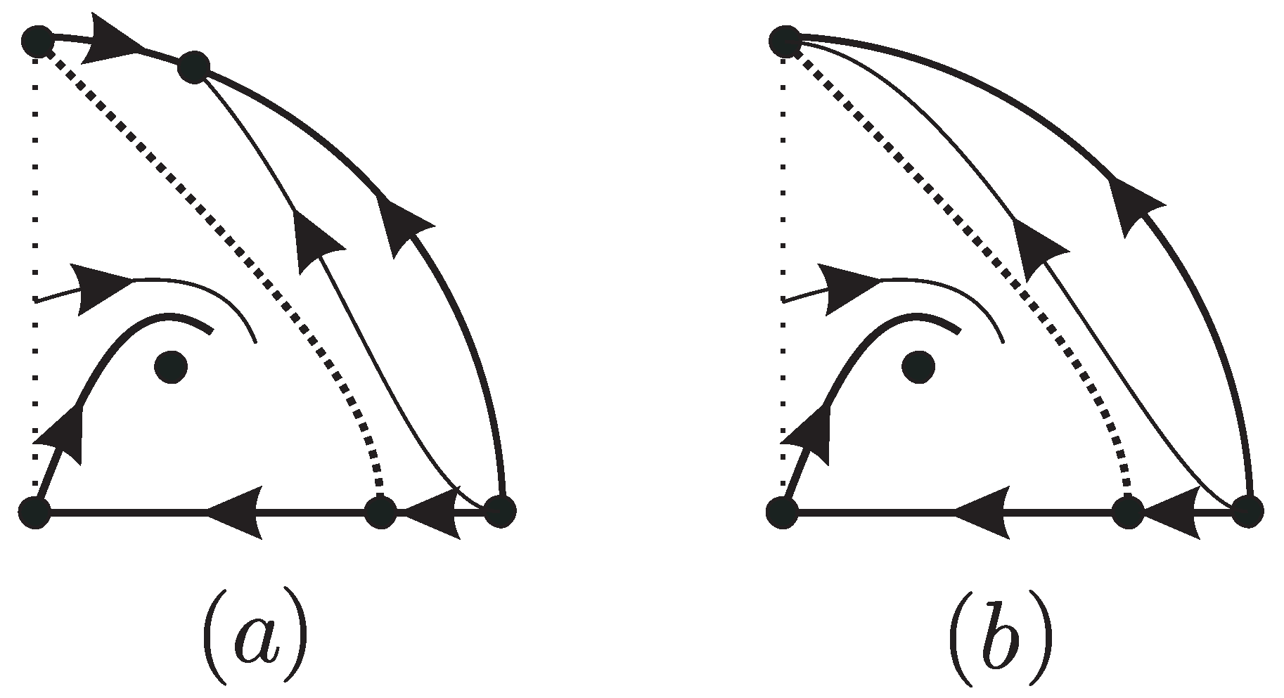
The phase portrait of the differential system (2) when

γ \in (1, 2)

is topologically equivalent to the phase portrait

γ_{15}

, and when

γ = 2

is topologically equivalent to the phase portrait

γ_{16}

. In order to pass from the phase portraits of system (2) to system (4) we must take into account the change in the time

d t = (1 - 2 x) d s

. Then the positive quadrants of the phase portraits

γ_{15}

and

γ_{16}

of system (2), pass to the positive quadrants of system (4) changing the direction of orbits in the region

x > 1 / 2

, and omitting the straight line

x = 1 / 2

where system (4) is not defined. In summary, the phase portraits in the positive quadrant Q of system (4) are shown in Figure 2.

Since

t = ln (r / R)

and r varies on the interval

(0, R]

, t varies in the interval

(- \infty, 0]

. Taking into account that the meaning of the variables x and y are

x = m (r) / r > 0

and

y = 4 π r^{2} ρ > 0

, from Figure 2 it follows that all the orbits which are in

Q_{1}

are positively invariant, and the ones which are in

Q_{2}

are invariant. So statement (a) is proved.

From Figure 2 all the orbits which are in

Q_{2}

satisfy that

\frac{m (r)}{r} \to \infty and 4 π r^{2} ρ \to 0,

(7)

when

t \to - \infty

, i.e. when

r \to 0

. This proves statement (b).

Q_{1}

there is the equilibrium point

P = (2 (γ - 1) / (γ^{2} + 4 γ - 4), 2 (γ - 1) / (γ^{2} + 4 γ - 4))

. So if

(m (R) / R, 4 π R^{2} ρ) = P

, then for all

r \in (0, R]

we have that

(m (r) / r, 4 π r^{2} ρ) = P

. So statement (c) is proved.

From Figure 2 all the orbits which are in

Q_{1}

, with the exception of the equilibrium point P, satisfy that

\frac{m (r)}{r} \to 0 and 4 π r^{2} ρ \to k \geq 0,

(8)

for some finite negative value of t, i.e. there is a positive value

r = r_{0} < R

for which (8) holds. This completes the proof of statement (d). Hence Theorem 2 is proved.

4. Conclusions

The differential system

\frac{d x}{d t} = y - x, \frac{d y}{d t} = \frac{y}{1 - 2 x} (2 - γ y - \frac{5 γ - 4}{γ - 1} x),

when the parameter

γ \in (1, 2]

models the structure equations of a static star in general relativity in the case of the existence of a homologous family of solutions, being

x = m (r) / r

where

m (r) \geq 0

is the mass inside the sphere of radius r of the star,

y = 4 π r^{2} ρ

where

ρ

is the density of the star, and

t = ln (r / R)

where R is the radius of the star. In Theorem 2 we have classified all the possible values of

m (r) / r

and

4 π r^{2} ρ

when

r \to 0

Acknowledgments

This work is supported by the Agencia Estatal de Investigación grant PID2019-104658GB-I00, and the H2020 European Research Council grant MSCA-RISE-2017-777911. The third author is partially supported by the grant number 21.70105.31 ŞD.

Appendix: Poincaré Compactification

In order to classify the global dynamics of a polynomial differential system the first crucial step is to characterize their finite and infinite equilibrium points in the Poincaré compactification. The second main step for determining the global dynamics in the Poincaré disc of a polynomial differential system is the characterization of their separatrices. For the polynomial differential systems in the Poincaré disc it is known that the separatrices are the infinite orbits, the finite equilibrium points, the separatrices of the hyperbolic sectors of the finite and infinite equilibrium points, and the limit cycles.

Σ

denotes the set of all separatrices in the Poincaré disc

D^{2}

Σ

is a closed set and the components of

D^{2} ∖ Σ

are called the canonical regions. We denote by S and R the number of separatrices and canonical regions, respectively.

We consider the set of all polynomial vector fields in

R^{2}

of the form

(\dot{x}, \dot{y}) = X (x, y) = (P (x, y), Q (x, y)),

(9)

where P and Q are real polynomials in the variables x and y of degrees

d_{1}

and

d_{2}

, respectively. Take

d = max {d_{1}, d_{2}}

Denote by

T_{p} S^{2}

be the tangent space to the 2-dimensional sphere

S^{2} = {s = (s_{1}, s_{2}, s_{3}) \in R^{3} : s_{1}^{2} + s_{2}^{2} + s_{3}^{2} = 1}

at the point p. Assume that X is defined in the tangent plane to

S^{2}

at the point

(0, 0, 1)

denoted by

T_{(0, 0, 1)} S^{2} = R^{2}

. Consider the central projection

f : T_{(0, 0, 1)} S^{2} \to S^{2}

. This map defines two copies of X, one in the open northern hemisphere and the other in the open southern hemisphere. Denote by

X^{'}

the vector field

D f \circ X

defined on

S^{2}

except on its equator

S^{1} = {s \in S^{2} : s_{3} = 0}

. Clearly

S^{1}

is identified to the infinity of

R^{2}

. If X is a planar polynomial vector field of degree d, then

p (X)

is the only analytic extension of

s_{3}^{d - 1} X^{'}

S^{2}

. The vector field

p (X)

is called the Poincaré compactification of the vector field X, for more details see ([6] chapter 5).

On the Poincaré sphere

S^{2}

we use the following six local charts, which are given by

U_{i} = {s \in S^{2} : s_{i} > 0}

and

V_{i} = {s \in S^{2} : s_{i} < 0}

, for

i = 1, 2, 3

, with the corresponding diffeomorphisms

φ_{i} : U_{i} \to R^{2}, ψ_{i} : V_{i} \to R^{2},

defined by

φ_{i} (s) = - ψ_{i} (s) = (s_{m} / s_{i}, s_{n} / s_{i}) = (u, v)

for

m < n

and

m, n \neq i

. Thus

(u, v)

will play different roles in the distinct local charts. The expressions of the vector field

p (X)

are

(\dot{u}, \dot{v}) = (v^{d} (Q (\frac{1}{v}, \frac{u}{v}) - u P (\frac{1}{v}, \frac{u}{v})), - v^{d + 1} P (\frac{1}{v}, \frac{u}{v})) in U_{1},

(\dot{u}, \dot{v}) = (v^{d} (P (\frac{u}{v}, \frac{1}{v}) - u Q (\frac{u}{v}, \frac{1}{v})), - v^{d + 1} Q (\frac{u}{v}, \frac{1}{v})) in U_{2},

(\dot{u}, \dot{v}) = (P (u, v), Q (u, v)) in U_{3} .

We note that the expressions of the vector field

p (X)

in the local chart

(V_{i}, ψ_{i})

is equal to the expression in the local chart

(U_{i}, ϕ_{i})

multiplied by

{(- 1)}^{d - 1}

for

i = 1, 2, 3

The orthogonal projection under

π (y_{1}, y_{2}, y_{3}) = (y_{1}, y_{2})

of the closed northern hemisphere of

S^{2}

onto the plane

s_{3} = 0

is a closed disc

D^{2}

of radius one centered at the origin of coordinates called the Poincaré disc. Since a copy of the vector field X on the plane

R^{2}

is in the open northern hemisphere of

S^{2}

, the interior of the Poincaré disc

D^{2}

is identified with

R^{2}

and the boundary of

D^{2}

, the equator

S^{1}

S^{2}

, is identified with the infinity of

R^{2}

. Consequently the phase portrait of the vector field X extended to the infinity corresponds to the projection of the phase portrait of the vector field

p (X)

on the Poincaré disc

D^{2}

The equilibrium points of

p (X)

in the Poincaré disc lying on

S^{1}

are the infinite equilibrium points of the corresponding vector field X. The equilibrium points of

p (X)

in the interior of the Poincaré disc, i.e. on

S^{2} ∖ S^{1}

, are the finite equilibrium points. We note that in the local charts

U_{1}

U_{2}

V_{1}

and

V_{2}

the infinite equilibrium points have their coordinate

v = 0

For a polynomial vector field (9) if

s \in S^{1}

is an infinite equilibrium point, then

- s \in S^{1}

is another infinite equilibrium point. Thus the number of infinite equilibrium points is even and the local phase portrait of one is that of the other multiplied by

{(- 1)}^{d + 1}

References

J.C. ARTÉS, J. LLIBRE, D. SCHLOMIUK AND N. VULPE, Geometric Configurations of Singularities of Planar Polynomial Differential Systems. A Global Classification in the Quadratic Case, Birkhäuser, 2021.
N.N. BAUTIN, On periodic solutions of a system of differential equations, Prikl. Mat. Meh. 18, (1954), 128.
C.G. BÖHMER, T. HARKO AND S.V. SABAU, Jacobi stability analysis of dynamical systems applications in gravitation and cosmology, Adv. Theor. Math. Phys. 16 (2012), 1145–1196.
S. CHANDRASEKHAR, An introduction to the study of stellar structure, Dover, New York, 1939. [CrossRef]
C.B. COLLINS, Static stars: Some mathematical curiosities, J. Math. Phys. 18 (1977), 1374–1377. [CrossRef]
F. DUMORTIER, J. LLIBRE AND J.C. ARTÉS, Qualitative theory of planar differential systems, UniversiText, Springer–Verlag, New York, 2006.
F. GAO AND J. LLIBRE, Global dynamics of the Hořava-Lifshitz cosmological system, General Relativity and Gravitation 51 (2019), 152–pp 15. [CrossRef]
J. GINÉ, N. KHAJOEI AND C. VALLS, Integrability of the Tolman-Oppenheimer-Volkoff equation, preprint, (2021).
J.M. GINOUX, J. LLIBRE, C. VALLS, Dynamics and Darboux integrability of the D₂ polynomial vector fields of degree 2 in R², Math. Phys. Anal. Geom. 24 (2021), 1, 16 pp. [CrossRef]
C.W. MISNER AND H.S. ZAPOLSKY, High-Density Behavior and Dynamical Stability of Neutron Star Model, Phys. Rev. Lett. 12 (1964), 635–637. Erratum Phys. Rev. Lett. 13, (1964), 122. [CrossRef]
J.W. REYN, hase portraits of planar quadratic systems, Mathematics and its Applications, vol. 583, Springer, New York, 2007.
D. SCHLOMIUK AND N. VULPE, Planar quadratic differential systems with invariant straight lines of at least five total multiplicity, Qual. Theory Dyn.Syst., 5, no. 1 (2004), 135–194. [CrossRef]
YE YANQUIAN ET AL., Theory of limit cycles, Translations of Mathematical Monographs, vol. 66, American Mathematical Society, Providence, RI, 1986.

Figure 1. Phase portraits of the quadratic systems (2).

Figure 2. Phase portrait in the positive quadrant of the quadratic systems (2): (a) for

γ \in (1, 2)

, and (b) for

γ = 2

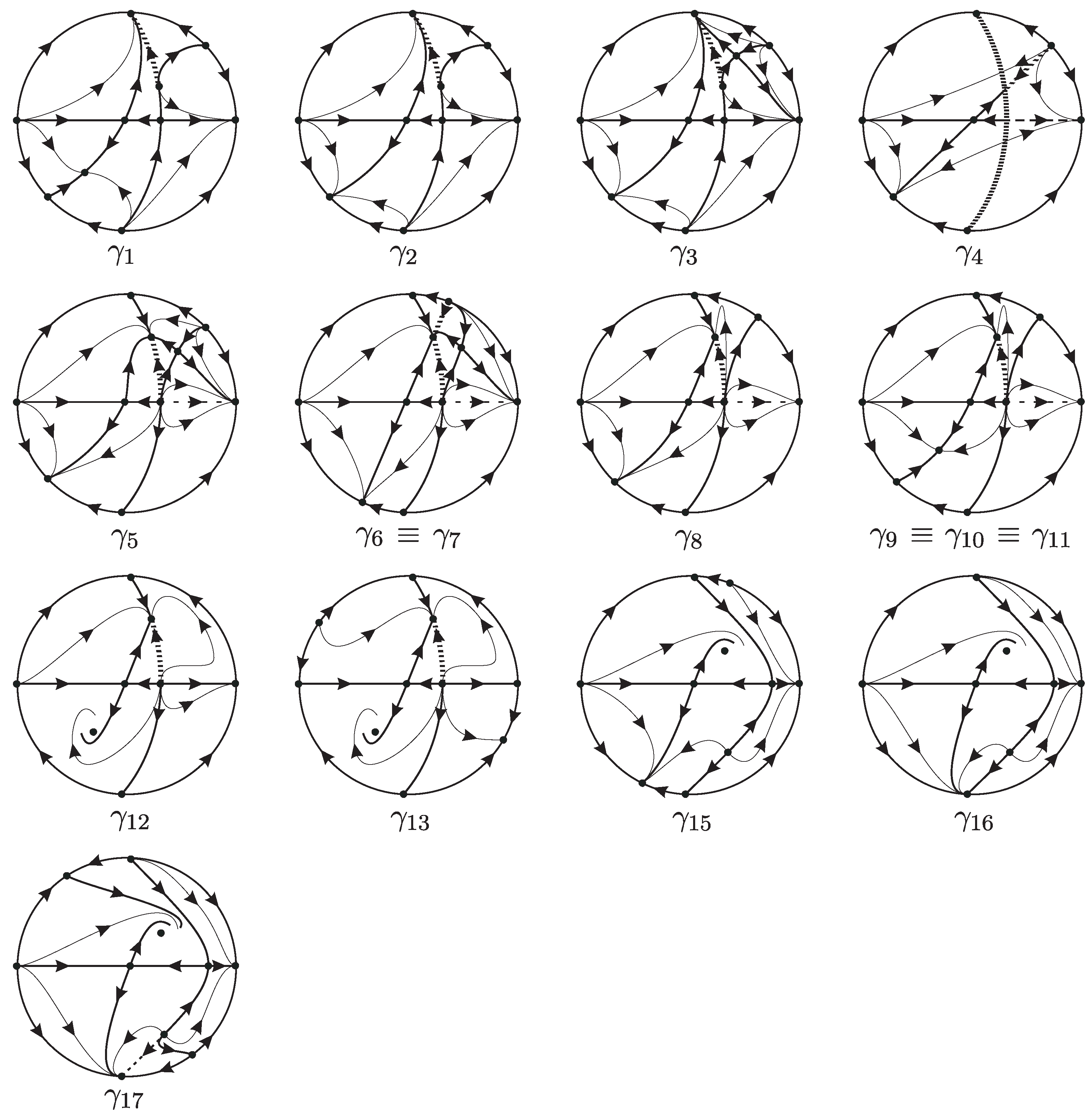
Figure 2. Phase portrait in the positive quadrant of the quadratic systems (2): (a) for

γ \in (1, 2)

, and (b) for

γ = 2

Disclaimer/Publisher’s Note: The statements, opinions and data contained in all publications are solely those of the individual author(s) and contributor(s) and not of MDPI and/or the editor(s). MDPI and/or the editor(s) disclaim responsibility for any injury to people or property resulting from any ideas, methods, instructions or products referred to in the content.

© 2023 by the authors. Licensee MDPI, Basel, Switzerland. This article is an open access article distributed under the terms and conditions of the Creative Commons Attribution (CC BY) license (http://creativecommons.org/licenses/by/4.0/).

Copyright: This open access article is published under a Creative Commons CC BY 4.0 license, which permit the free download, distribution, and reuse, provided that the author and preprint are cited in any reuse.

MDPI Initiatives

Important Links

Choose an area of interest and we will send you notifications of new preprints at your preferred frequency.

Disclaimer

Dynamics of the Static Star Differential System from the Mathematical and Physical Point of Views

Abstract

1. Introduction and the Main Results

2. Proof of Theorem 1

3. Proof of Theorem 2

4. Conclusions

Acknowledgments

Appendix: Poincaré Compactification

References

MDPI Initiatives

Important Links

Subscribe