Submitted:
23 October 2023
Posted:
23 October 2023
You are already at the latest version
Abstract
Keywords:
1. Introduction
2. Methodology
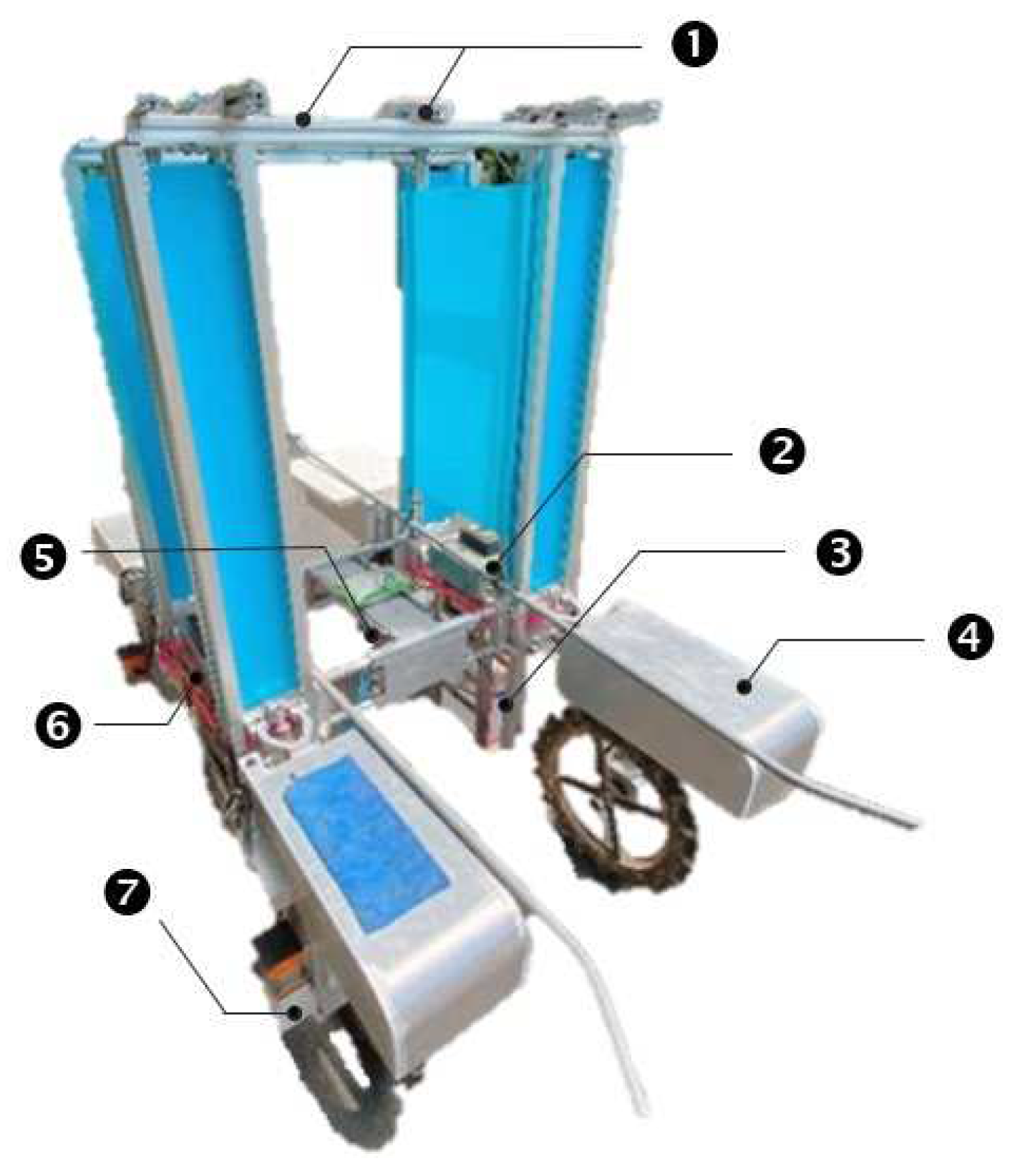
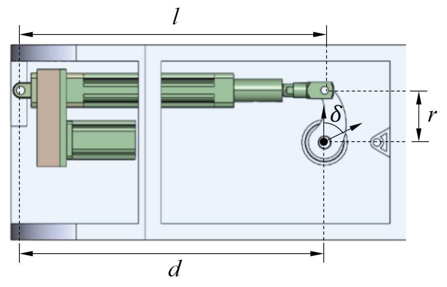
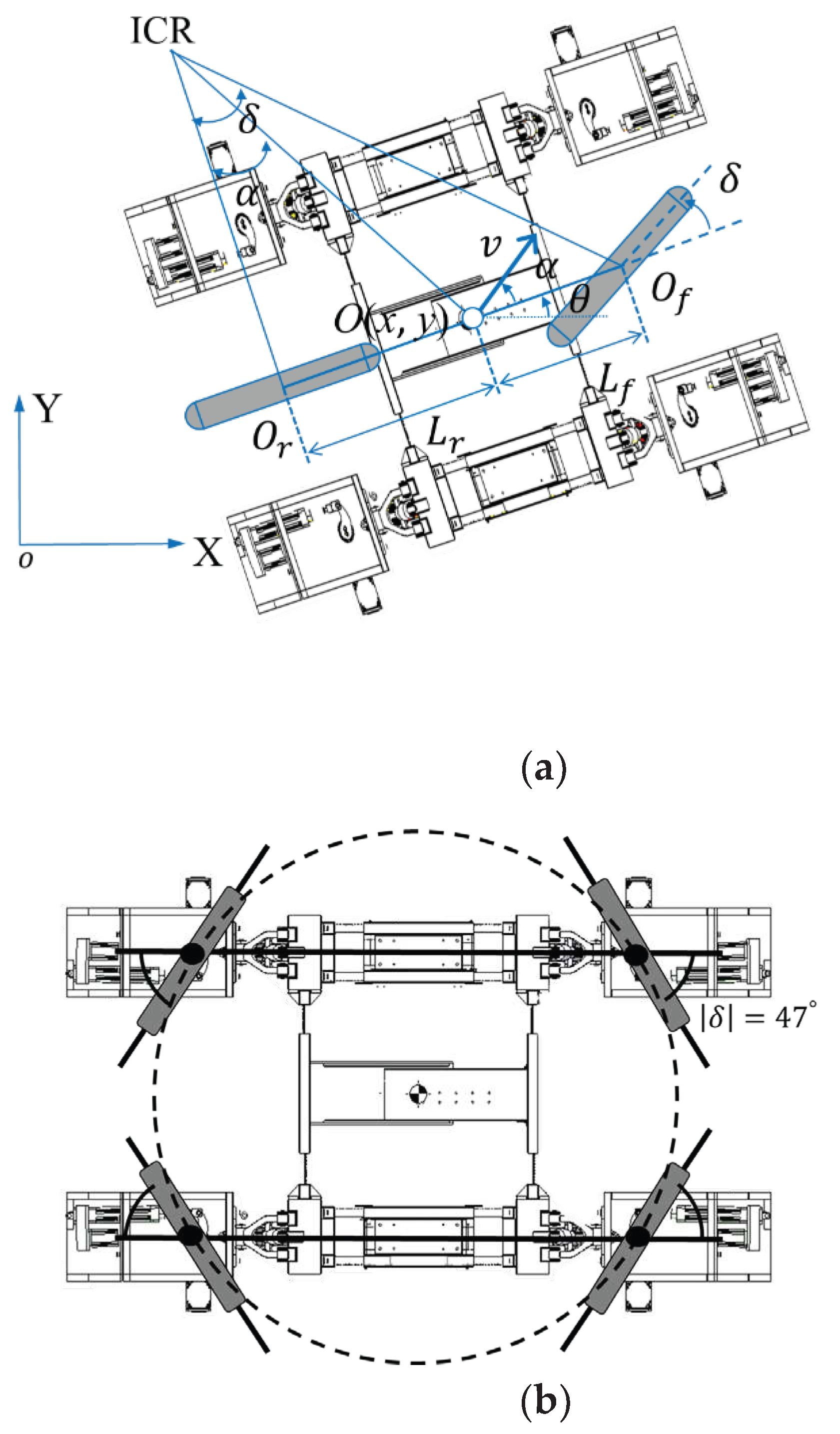
2.1. Agriculture Robot Design
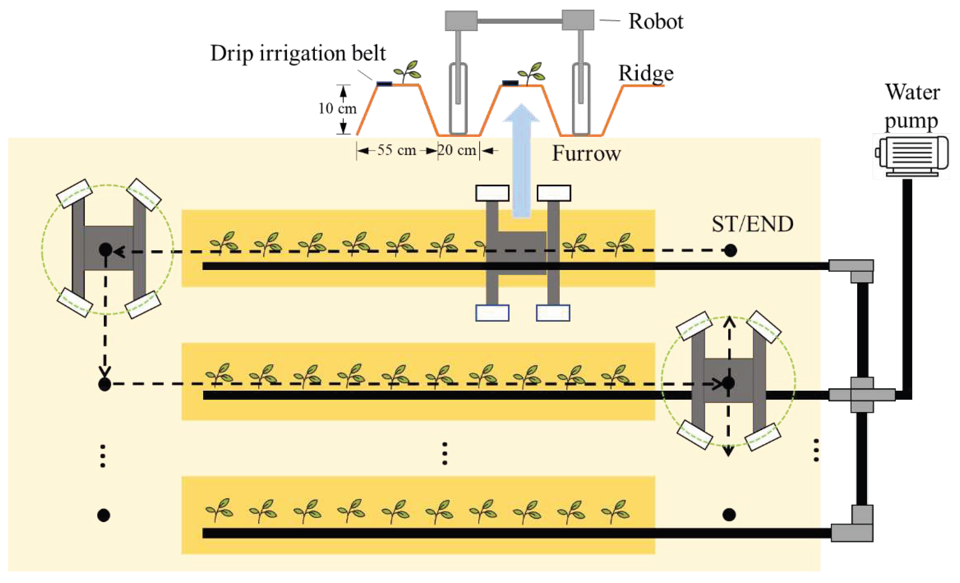
2.2. Path Planning
2.3. Row Detection
2.4. Guidance and Heading Control
2.4.1. Velocity Measurement
2.4.2. Heading Angle Measurement
- Fuzzification process;
- Knowledge base;
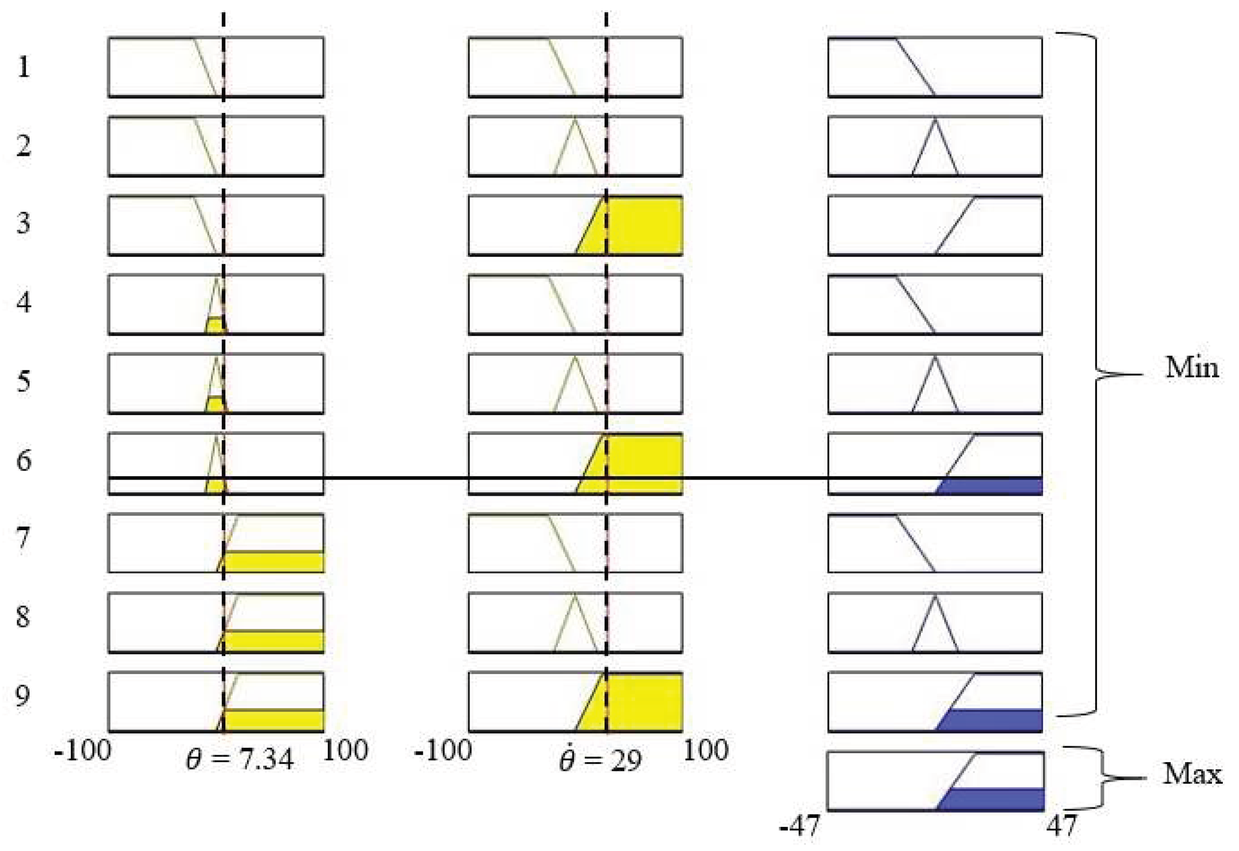
- Rule 1: IF ( is LO) AND ( is N) THEN ( is L)
- Rule 2: IF ( is LO) AND ( is Z) THEN ( is M)
- Rule 3: IF ( is LO) AND ( is P) THEN ( is R)
- Rule 4: IF ( is M) AND ( is N) THEN ( is L)
- Rule 5: IF ( is M) AND ( is Z) THEN ( is M)
- Rule 6: IF ( is M) AND ( is P) THEN ( is R)
- Rule 7: IF ( is RO) AND ( is N) THEN ( is L)
- Rule 8: IF ( is RO) AND ( is Z) THEN ( is M)
- Rule 9: IF ( is RO) AND ( is P) THEN ( is R)
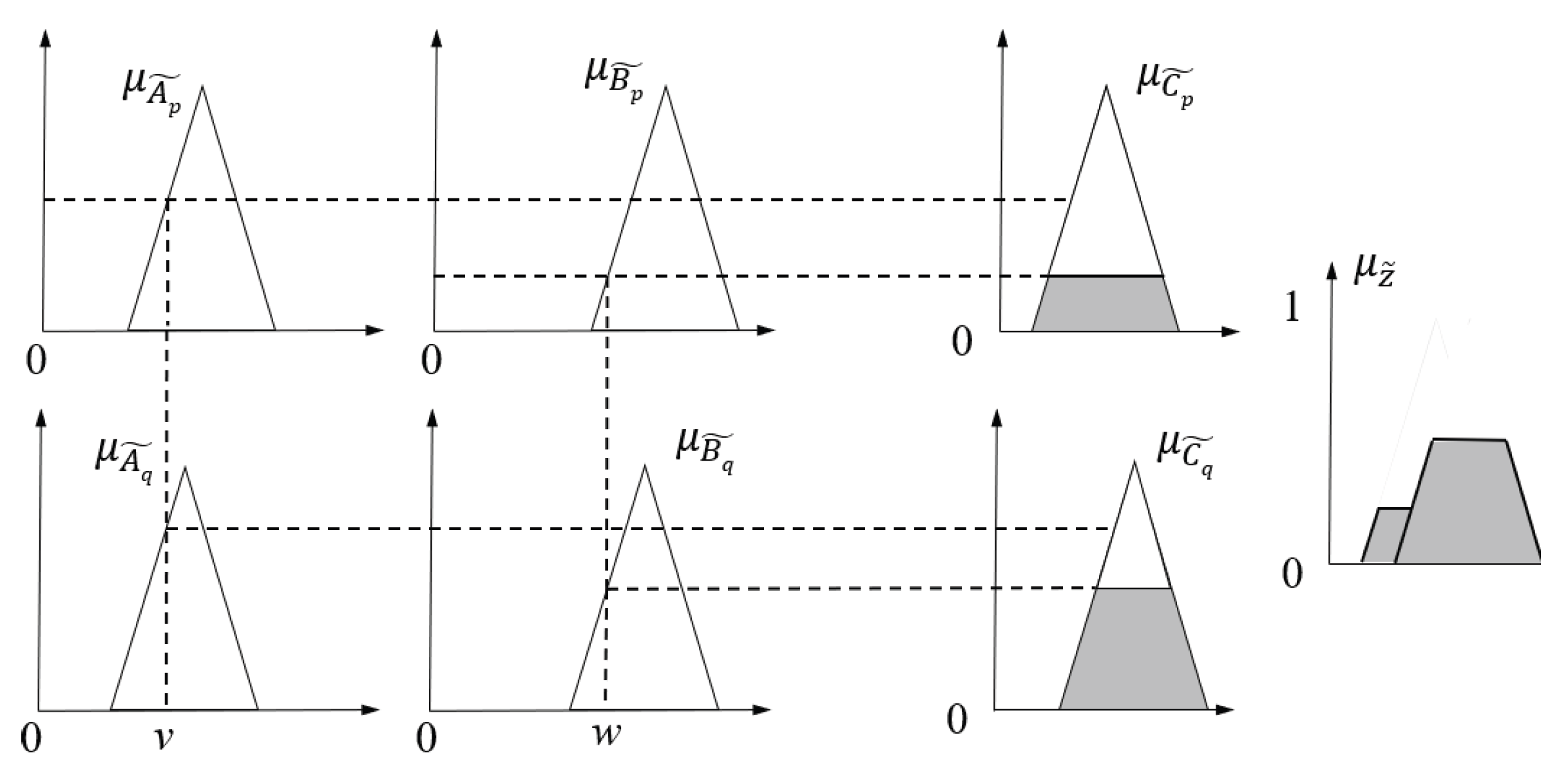
- Fuzzy inference and decision;
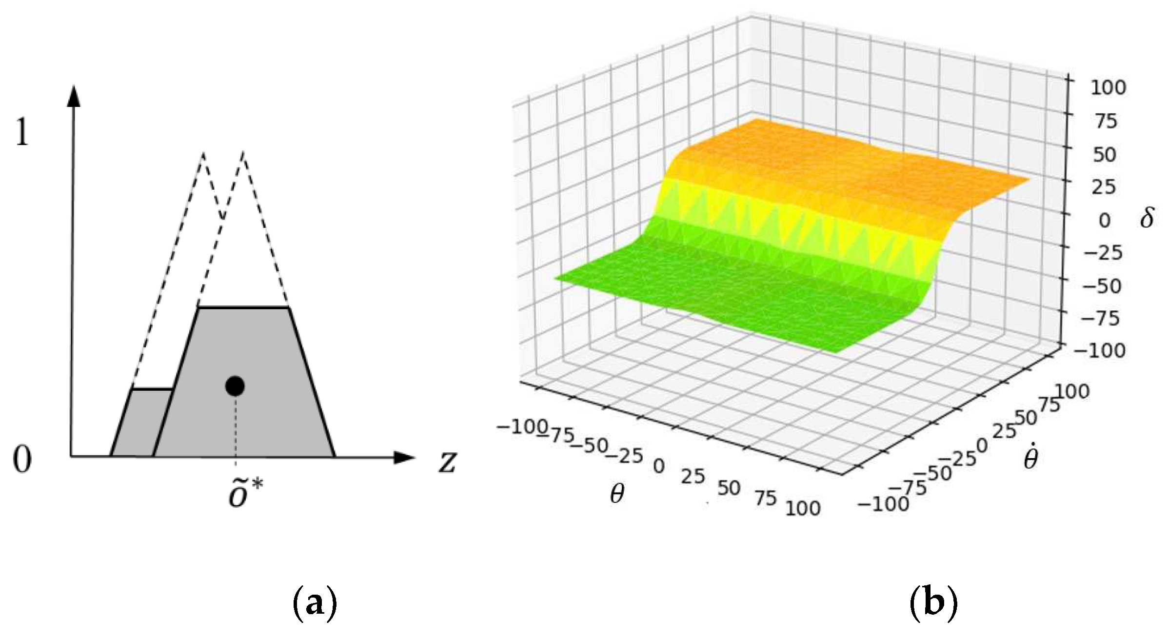
- Defuzzification.
3. Results and Discussion
3.1. Environmental Conditions and Experimental Parameters
3.2. Initial Test
3.3. Experimental Results
3.3.1. Autonomous Guidance
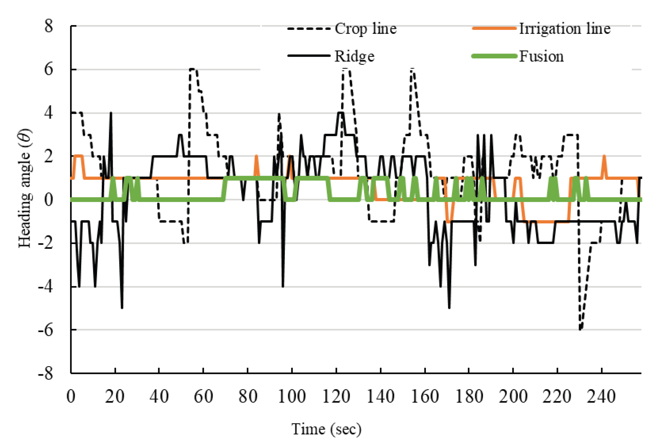
| Type of Guidance Line | Sunny | Sunny and Cloudy | Cloudy |
|---|---|---|---|
| Irrigation line | ±3 | ±2 | ±2 |
| Crop line | ±6 | ±6 | ±6 |
| Ridge line | ±6 | ±3 | ±4 |
| Fusion | ±2 | ±2 | ±1 |
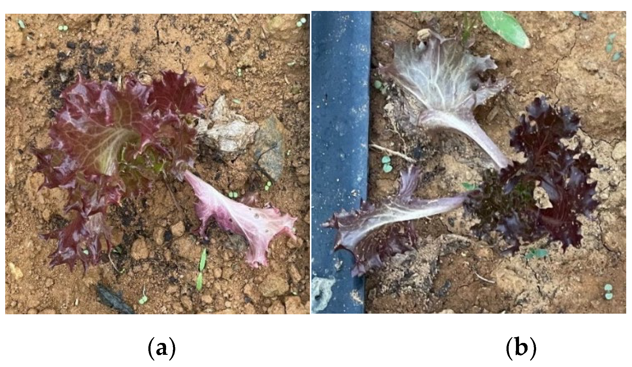
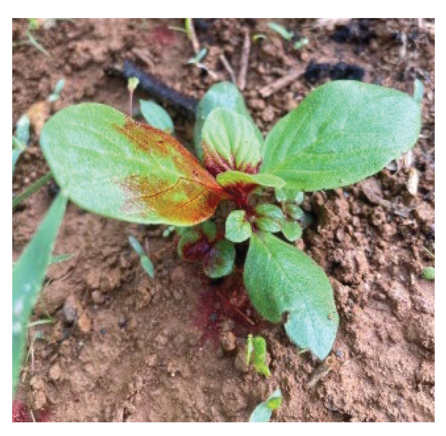
3.3.2. Identification of Weed and Crop Nutrient Deficiency Symptoms
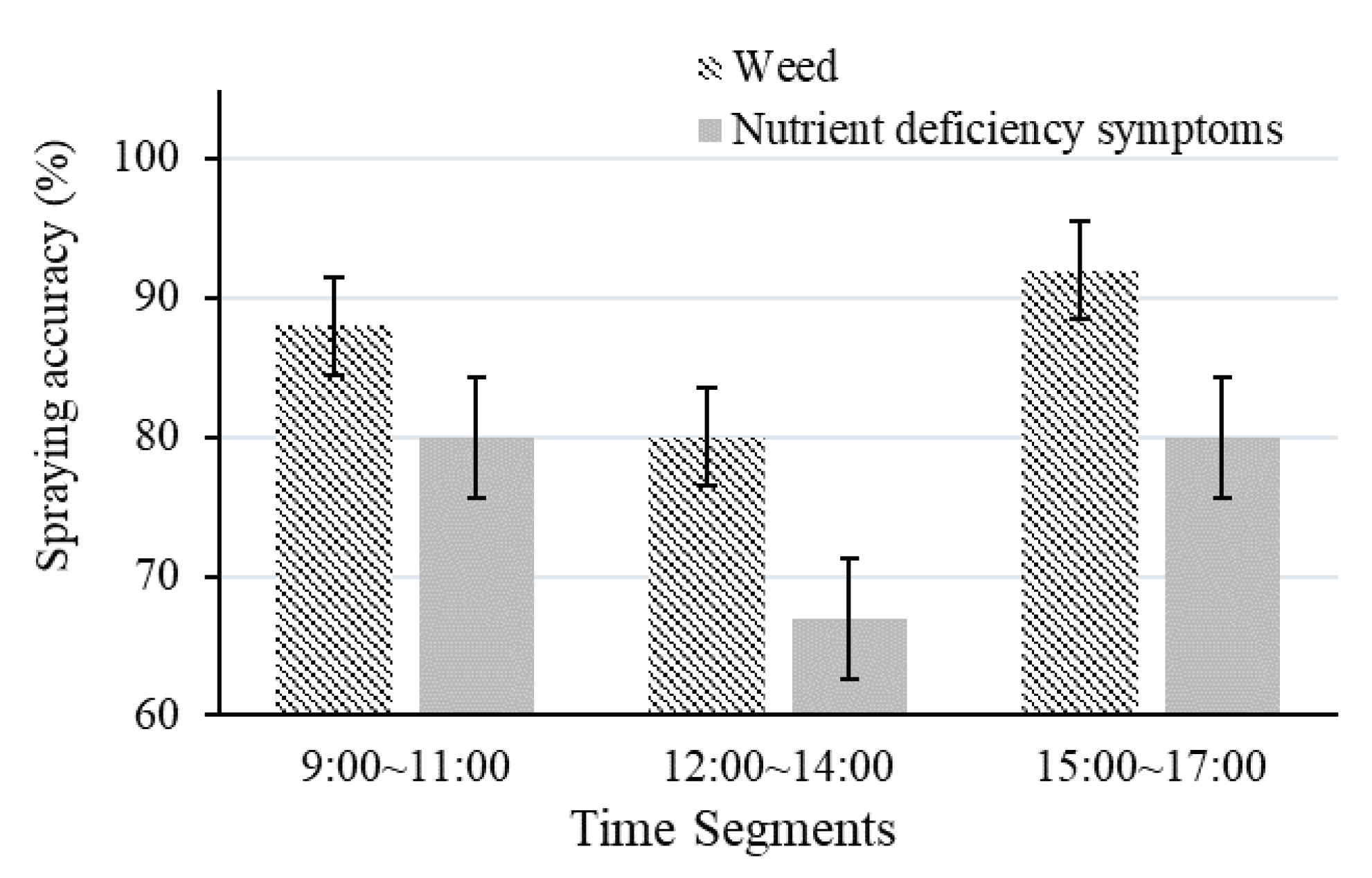
3.3.3. Spray Test
3.3.4. Discussion
4. Conclusions
Author Contributions
Funding
Institutional Review Board Statement
Informed Consent Statement
Conflicts of Interest
References
- Spykman, O.; Gabriel, A.; Ptacek, M.; Gandorfer, M. Farmers’ perspectives on field crop robots—Evidence from Bavaria, Germany. Comput. Electron. Agric. 2021, 186, 106176. [Google Scholar] [CrossRef]
- Wu, J.; Jin, Z.; Liu, A.; Yu, L.; Yang, F. A survey of learning-based control of robotic visual servoing systems. J. Franklin Inst. 2022, 359, 556–577. [Google Scholar] [CrossRef]
- Kato, Y.; Morioka, K. Autonomous robot navigation system without grid maps based on double deep Q-Network and RTK-GNSS localization in outdoor environments. 2019 IEEE/SICE Int. Symp. Syst. Integration (SII), Paris, France, 346–351.
- Galati, R.; Mantriota, G.; Reina, G. RoboNav: An affordable yet highly accurate navigation system for autonomous agricultural robots. Robotics 2022, 11, 99. [Google Scholar] [CrossRef]
- Chien, J.C.; Chang, C.L.; Yu, C.C. Automated guided robot with backstepping sliding mode control and its path planning in strip farming. Int. J. iRobotics 2022, 5, 16–23. [Google Scholar]
- Tian, H.; Wang, T.; Liu, Y.; Qiao, X.; Li, Y. Computer vision technology in agricultural automation—A review. Inf. Process. Agric. 2020, 7, 1–19. [Google Scholar] [CrossRef]
- Choi, K.H.; Han, S.K.; Han, S.H.; Park, K.-H.; Kim, K.-S.; Kim, S. Morphology-based guidance line extraction for an autonomous weeding robot in paddy fields. Comput. Electron. Agric. 2015, 113, 266–274. [Google Scholar] [CrossRef]
- Suriyakoon, S.; Ruangpayoongsak, N. Leading point-based interrow robot guidance in corn fields. 2017 2nd Int. Conf. Control Robotics Eng. (ICCRE), Bangkok, Thailand, 8–12.
- Bonadiesa, S.; Gadsden, S.A. An overview of autonomous crop row navigation strategies for unmanned ground vehicles. Eng. Agric. Environ. Food 2019, 12, 24–31. [Google Scholar] [CrossRef]
- Chen, J.; Qiang, H.; Wu, J.; Xu, G.; Wang, Z. Navigation path extraction for greenhouse cucumber-picking robots using the prediction-point Hough transform. Comput. Electron. Agric. 2021, 180, 105911. [Google Scholar] [CrossRef]
- Shi, J.; Bai, Y.; Diao, Z.; Zhou, J.; Yao, X.; Zhang, B. Row detection-based navigation and guidance for agricultural robots and autonomous vehicles in row-crop fields: Methods and applications. Agronomy 2023, 13, 1780. [Google Scholar] [CrossRef]
- Ruan, Z.; Chang, P.; Cui, S.; Luo, J.; Gao, R.; Su, Z. A precise crop row detection algorithm in complex farmland for unmanned agricultural machines. Biosyst. Eng. 2023, 232, 1–12. [Google Scholar] [CrossRef]
- Zhang, S.; Wang, Y.; Zhu, Z.; Li, Z.; Du, Y.; Mao, E. Tractor path tracking control based on binocular vision. Inf. Process. Agric. 2018, 5, 422–432. [Google Scholar] [CrossRef]
- Mavridou, E.; Vrochidou, E.; Papakostas, G.A.; Pachidis, T.; Kaburlasos, V.G. Machine vision systems in precision agriculture for crop farming. J. Imaging 2019, 5, 89. [Google Scholar] [CrossRef] [PubMed]
- Gu, Y.; Li, Z.; Zhang, Z.; Li, J.; Chen, L. Path tracking control of field information-collecting robot based on improved convolutional neural network algorithm. Sensors 2020, 20, 797. [Google Scholar] [CrossRef] [PubMed]
- Suriyakoon, S.; Ruangpayoongsak, N. Leading point-based interrow robot guidance in corn fields. 2017 2nd Int. Conf. Control Robotics Eng. (ICCRE), Bangkok, Thailand, 8–12.
- Pajares, G., García-Santillán, I., Campos, Y., Montalvo, M., Guerrero, J.M., Emmi, L., Romeo, J., Guijarro, M., & González-de-Santos, P., Machine-vision systems selection for agricultural vehicles: A guide. J. Imaging 2016, 2, 34.
- RegenerateHu, Y.; Huang, H. Extraction method for centerlines of crop row based on improved lightweight Yolov4. 2021 6th International Symposium on Computer and Information Processing Technology (ISCIPT), Changsha, China, 127–132, 2021.
- de Silva, R.; Cielniak, G.; Gao, J. (2021). Towards agricultural autonomy: Crop row detection under varying field conditions using deep learning. arXiv preprint arXiv:2109.08247. arXiv:2109.08247.
- Hu, D.; Ma, C.; Tian, Z.; Shen, G.; Li, L. Rice Weed detection method on YOLOv4 convolutional neural network. 2021 International Conference on Artificial Intelligence, big data and algorithms (CAIBDA), 41–45.
- Ruigrok, T.; van Henten, E.; Booij, J.; van Boheemen, K.; Kootstra, G. Application-specific evaluation of a weed-detection algorithm for plant-specific Spraying. Sensors 2020, 20, 7262. [Google Scholar] [CrossRef] [PubMed]
- Chang, C.L.; Xie, B.X.; Chung, S.C. Mechanical control with a deep learning method for precise weeding on a farm. Agriculture 2021, 11, 1049. [Google Scholar] [CrossRef]
- Wang, Q.; Cheng, M.; Huang, S.; Cai, Z.; Zhang, J.; Yuan, H. A deep learning approach incorporating YOLO v5 and attention mechanisms for field real-time detection of the invasive weed Solanum rostratum Dunal seedlings. Comput. Electron. Agric. 2022, 199, 107194. [Google Scholar] [CrossRef]
- Chen, J.; Wang, H.; Zhang, H.; Luo, T.; Wei, D.; Long, T.; Wang, Z. Weed detection in sesame fields using a YOLO model with an enhanced attention mechanism and feature fusion. Comput. Electron. Agric. 2022, 202, 107412. [Google Scholar] [CrossRef]
- Farooq, U.; Rehman, A.; Khanam, T.; Amtullah, A.; Bou-Rabee, M.A.; Tariq, M. Lightweight deep learning model for weed detection for IoT devices. In Proceedings of the 2022 2nd International Conference on Emerging Frontiers in Electrical and Electronic Technologies (ICEFEET), Patna, India; 2022; pp. 1–5. [Google Scholar]
- Ruigrok, T.; van Henten, E.J.; Kootstra, G. Improved generalization of a plant-detection model for precision weed control. Comput. Electron. Agric. 2023, 204, 107554. [Google Scholar] [CrossRef]
- Suriyakoon, S.; Ruangpayoongsak, N. Leading point based interrow robot guidance in corn fields. In Proceedings of the 2017 2nd International Conference on Control and Robotics Engineering (ICCRE), Bangkok, Thailand, 8–12.
- Qiu, Q.; Fan, Z.; Meng, Z.; Zhang, Q.; Cong, Y.; Li, B.; Wang, N.; Zhao, C. Extended Ackerman steering principle for the co-ordinated movement control of a four wheel drive agricultural mobile robot. Comput. Electron. Agric. 2018, 152, 40–50. [Google Scholar] [CrossRef]
- Bonadiesa, S.; Gadsden, S.A. An overview of autonomous crop row navigation strategies for unmanned ground vehicles. Eng. Agric. Environ. Food 2019, 12, 24–31. [Google Scholar] [CrossRef]
- Tu, X.; Gai, J.; Tang, L. Robust navigation control of a 4WD/4WS agricultural robotic vehicle. Comput. Electron. Agric. 2019, 164, 104892. [Google Scholar] [CrossRef]
- Zhang, L.; Zhang, R.; Li, L.; Ding, C.; Zhang, D.; Chen, L. Research on virtual Ackerman steering model based navigation system for tracked vehicles. Comput. Electron. Agric. 2022, 192, 106615. [Google Scholar] [CrossRef]
- Bennett, P. The NMEA FAQ (Fragen und Antworten zu NMEA), Ver. 6.1, Sep. 1997.
- Shih, P.T.-Y. TWD97 and WGS84, datum or map projection? J. Cadastral Survey 2020, 39, 1–12. [Google Scholar]
- Chang, C.L.; Chen, H.W. Straight-line generation approach using deep learning for mobile robot guidance in lettuce fields. In Proceedings of the 2023 9th International Conference on Applied System Innovation (ICASI).
- Bochkovskiy, A.; Wang, C.-Y.; Liao, H.-Y. M. YOLOv4: Optimal speed and accuracy of object detection. arXiv:2004.10934. arXiv:2004.10934.
- Wang, C.Y.; Liao, H.Y. M.; Wu, Y.H.; Chen, P.Y.; Hsieh, J.W.; Yeh, I.H. CSPNet: A new backbone that can enhance learning capability of CNN. In Proceedings of the 2020 IEEE/CVF Conference on Computer Vision and Pattern Recognition Work-shops (CVPRW), Seattle, WA, USA, 1571–1580.
- Zheng, Z.; Wang, P.; Liu, W.; Li, J.; Ye, R.; Ren, D. Distance-IoU loss: Faster and better learning for bounding box regression. AAAI Technical Track: Vision 2020, 34, 12993–13000. [Google Scholar] [CrossRef]
- Murphy, K.P. Machine learning: A probabilistic perspective, MIT press, 2012.
- Lee, C.C. Fuzzy logic in control system: Fuzzy logic controller. I. IEEE Trans. Syst. Man Cybern. 1990, 20, 404–418. [Google Scholar] [CrossRef]
- Meimetis, D., Daramouskas, I., Perikos, I.; Hatzilygeroudis, I. Real-time multiple object tracking using deep learning methods. Neural Comput. & Applic. 2023, 35, 89–118.

| Type | |||
| PID |
| Input Variable | Output Variable | |||||||
|---|---|---|---|---|---|---|---|---|
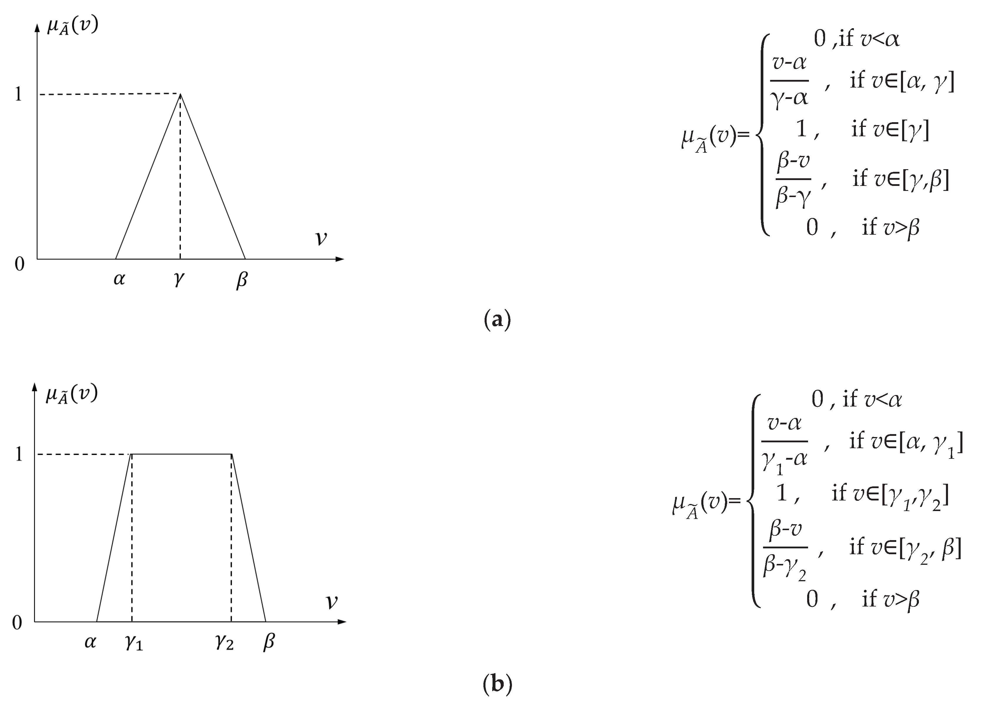
| Heading Angle (θ) | ) | Steering Angle (δ) | ||||||
| Crisp Interval | Linguistic Labels | Crisp Interval | Linguistic Labels | Crisp Interval | Linguistic Labels | |||
| Triangular ] |
Ladder ] |
Triangular [α, γ, β ] |
Ladder ] |
Triangular ] |
Ladder ] |
|||
| – | [-100, -100, -20, 0] | LO | – | [-100, -100, -25, 0] | N | – | [-17, -17, -7, 0] | L |
| [-10, 0, 10] | – | M | [-20, 0, 20] | – | Z | [-5, 0, 5] | – | M |
| – | [0, 20, 100, 100] | RO | – | [0, 25, 100, 100] | P | – | [0, 7, 17, 17] | R |
| Type | Average precision (%) | Recall (%) | F1-Score (%) |
|---|---|---|---|
| Black drip irrigation belt | 99.2 | 99.0 | 96.0 |
| Crop | 99.1 | 99.0 | 96.3 |
| Ridge | 98.5 | 99.0 | 96.1 |
| Crop with nutritional deficiencies | 90.0 | 81.3 | 85.4 |
| Weed | 91.2 | 84.2 | 88.5 |
Disclaimer/Publisher’s Note: The statements, opinions and data contained in all publications are solely those of the individual author(s) and contributor(s) and not of MDPI and/or the editor(s). MDPI and/or the editor(s) disclaim responsibility for any injury to people or property resulting from any ideas, methods, instructions or products referred to in the content. |
© 2023 by the authors. Licensee MDPI, Basel, Switzerland. This article is an open access article distributed under the terms and conditions of the Creative Commons Attribution (CC BY) license (http://creativecommons.org/licenses/by/4.0/).


