
Submitted:
27 September 2023
Posted:
28 September 2023
You are already at the latest version
Abstract
We consider a classial case of irrational integrals containing a square root of a quadratic polynomial. It is well known that they can be expressed in terms of elementary functions by one of three Euler’s substitutions. It is less known that the Euler substittutions have a beautiful geometric interpretation. In the framework of this interpretation one can see that the number 3 is not the most suitable. We show that it is natural to introduce the fourth Euler substitution. By the way, it is not clear who was the first to attribute these three substitutions to Euler. In his original treatise Leonhard Euler uses two substitutions which are sufficient to cover all cases.
Keywords:
integral calculus
; irrational integrals
; conics
; rational parameterization
; fourth Euler’s substitution
1. Introduction
Integrals of rational functions can be expressed in terms of elementary functions. Therefore a natural method of integration consists in using suitable substitutions and integration by parts to reduce our problem to integration of rational functions.
In this paper we consider irrational integrals containing the quadratic root of a quadratic polynomial, i.e., integrals of the form
where R is a rational fuction (a quotient of two polynomials) of x and y, and
The subject is, in principle, known. A standard method to deal with such integrals consists in using one of the so called Euler’s substitutions [1,2]. However, there are some details which need to be clarified. We will describe in detail a geometric approach to this problem and explain how many Euler substitutions actually exist.
In fact, to our beest knowledge, all sources mention exactly three types of substitutions in this context. It is not clear who was the first to introduce such classification. Euler substitutions are usually introduced and discussed in Russian sources, see, e.g., [3,4,5] (Leonhard Euler, although of Swiss origin, lived and worked in Saint Petersburg for many years). Surprisingly enough, the three substitutions appeared also in an old textbook by a Harvard professor, [6], without any reference to Euler.
In our paper we present a clear geometric intepretation of this problem, shortly mentioned in some sources, mainly of Russian origin [2,7]. The textbook [7] is not translated into English. Another book by the same author, [3], does not mention this geometric approach in the section on Euler’s substitutions.
The main novelty of this paper is the introduction of the fourth Euler substitution, which is a natural consequence of the geometric approach discussed in our paper.
2. Three classical Euler’s substitutions
The main idea of Euler’s substitutions consists in expressing as a linear function of x and a new parameter t in such a way that the resulting equation is linear with respect to x. In this paper we use the most common numbering of these three substitutions, compare [1,2,3,4,6]. In some sources a different order is used, see [5,8,9].
2.1. First Euler substitution
This substitution can be done only in the case :
Squaring both sides we get:
Terms quadratic in x cancel out and the resulting equation is linear in x. Computing x, we get a rational dependence on t:
2.2. Second Euler substitution
This substitution can be done only in the case :
Squaring both sides we get:
The constant c cancels out and dividing both sides by x we again derive an equation linear in x. Hence, similarly as in the previous case,
2.3. Third Euler substitution
This substitution can be done only in the case , where
is the discriminant of the quadratic polynomial. Then the polynomial has two distinct real roots and , and the third Euler substitution is given by:
Squaring both sides we get:
2.4. Original Euler’s approach
It is interesting that Leonhard Euler himself in his famous monograph used only two of these substitutions, see [10]. He considered two cases: and . In the first case () he proposed the substitution (6), while in the second case () he proposed the substitution (3) in a slightly modified form:
Obviously, the case is not included because then the quadratic polynomial is a square of the linear function in x and y is linear is x as well. Hence the integrand in (1) is rational in x from the very beginning.
3. Geometric interpretation
It is convenient to square both sides of represent (2) obtaining the equation of a quadratic curve
We will denote this curve (a conic section) by , i.e.,
3.1. Elliptic case:
The canonical form of the quadratic polynomial yields:
We can distinguish three cases, depending on the sign of the discriminant :
Only in the last case we get a non-degenerated quadratic curve.
3.2. Parabolic case:
For (and ) the conic is a parabola with the symmetry axis .
3.3. Hyperbolic case:
The canonical form of the quadratic polynomial yields:
We can distinguish three cases, depending on the sign of the discriminant :
Therefore, for we get a non-degenerated quadratic curve.
3.4. Rational parameterization – standard approach
The key idea leading to a rational parameterization consists in fixing an arbitrary point on the conic and assigning to any other point of this conic the line . Taking as a parameter t the slope of this line we obtain a rational parameterization of the conic [2,7]. Thus we have the system of three equations:
The points and belong to the conic and t is the slope of the straight line passing through and . Subtracting the second equation from the first one we get:
Substituting the last equation into the first one we obtain:
Assuming , we get
Now, the first and the last equation form a system of two linear equations for two variables , which can be solved in the standard way. As a result we obtain:
which means that we expressed x and y as rational functions of the parameter t.
Corollary 3.1.
There are infinitely many Euler-like substitutions. Each of them is determined by the choice of , provided that . Then the point is given by:
and other points are parameterized by (28).
In particular, the second Euler substitution corresponds to (provided that the graph of the quadric intersects the axis y), see Figure 1 and Figure 2. The third Euler substitution corresponds to being a root of the polynomial (provided that the graph of intersects the axis x), see Figure 3 and Figure 4.
The first Euler substitution apparently does not fit this picture. However, its geometric interpretation is even simpler and more evident. The formula (3) describes the family of lines parallel to asymptotes of the corresponding hyperbola, see Figure 5. We may treat it as a special case of (28) when the point lies at infinity. Note that points belong to the conic (15) in the limit for .
4. New insights from the geometric interpretation
The description given in the previous section is more or less known (see, e.g., [2,7]), although we are not aware about any reference containing all these details. We are going to derive from this geometric picture more quite interesting consequnces.
First of all, we identify characteristic points on the graph of a quadratic curve which can be chosen as in the most natural way: vertices (, , , ) and intersections with coordinate axes (, , , ), see Figure 6 and Figure 7.
In particular, in the case of the second Euler substitution (see Figure 1 and Figure 2) or , while in the case of the third Euler substitution (see Figure 3) or (see Figure 4). The first Euler substitution is related to at infinity.
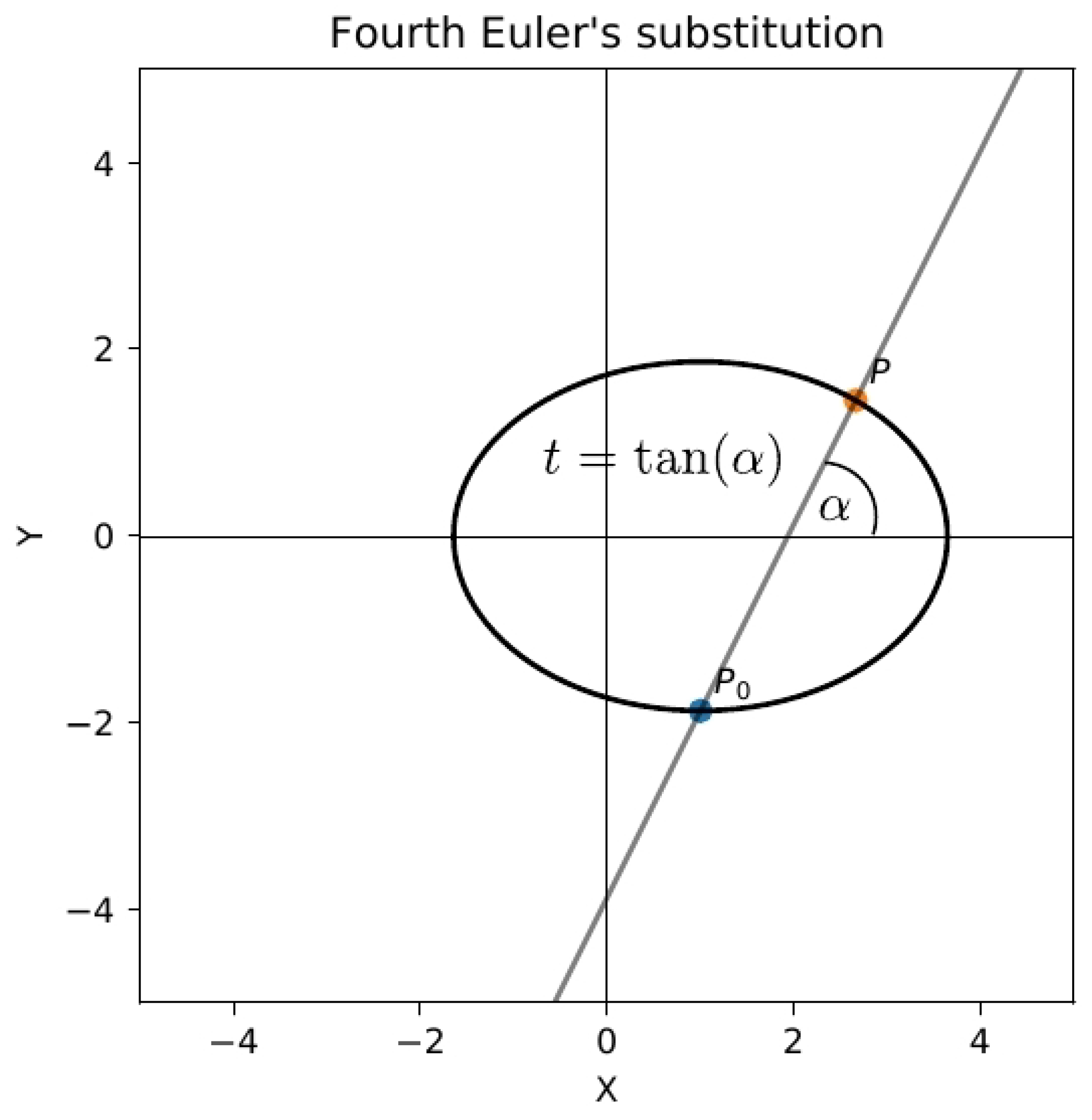
4.1. Fourth Euler’s substitution
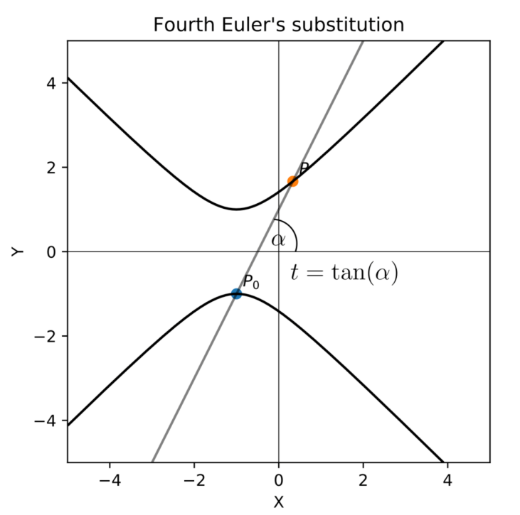
The geometric approach presented above includes all three classical Euler’s substitutions, but it is still missing vertices and . Therefore, it is natural to introduce another (fourth) Euler’s substitution, geometrically related to missing vertices: (see Figure 8 and Figure 9) or .
The algebraic description of the fourth Euler substitution is based on the canonical form of the quadratic polynomial:
where
The fourth Euler substitution is defined by:
Squaring both sides we get:
The constant q cancels out and dividing both sides by , we obtain
which is linear in x. Hence
and using (32) we get
Thus we have a rational dependence of x and y on the parameter t. Moreover,
and we can easily transform the irrational integral function (1) into an integral function rational with respect to t.
4.2. Rational parameterization – other parameters
Geometric approach suggests also some modifications or new variants of the existing rational parameterizations. Here we confine ourselves to one example. Introducing a new parameter
and substituting it into (4) and (5), we obtain the following simplification of the first Euler substitution:
Geometrically, the parameter t is related to intersections with the y axis (compare Figure 5), while the parameter is related to intersections with the vertical symmetry axis (i.e., the line ). Indeed, the parameter corresponds to the line passing through the point and this is one of two asymptotes (that is why and for ).
5. Euler’s substitutions versus trigonometric substitutions
Another popular method for computing irrational integrals (1) consists in making a suitable trigonometric or hyperbolic substitution. We use the canonical form of the quadratic curve (compare (30)):
Assuming (otherwise y depends linearly on x) we introduce new variables as folows:
Then (40) becomes
because , etc.
Thus we have three separate cases (in the fourth case –both signs negative– there are no real solutions), where trigonometric or hyperbolic substitutions are well known:
Is it better than Euler’s substitutions? This is a matter of taste. Perhaps it is more easy to memorize, however, one has to remember that integrals of trigonometric or hyperbolic functions have to be converted into integrals of rational functions by another substitution:
6. Conclusions
We presented and discussed a geometric approach to Euler substitutions. One consequence of this thorough discussion was the introduction of the fourth Euler substitution in addition to three traditionally mentioned Euler substitutions. In fact, we can say about infinite number (one parameter family) of Euler-like substitutions. They can be further modified or simplified by suitable linear or fractional linear transformations.
Surprisingly enough, the subject of constructing rational parametrization of algebraic curves (rationalizing roots) became recently important in the context of Feynman integrals and computations in high energy particle physics [11,12]. It would be interesting to appply in this field geometric ideas presented in our paper.
Author Contributions
Conceptualization, J.L.C.; methodology, J.L.C.; formal analysis, J.L.C. and M.J.; investigation, J.L.C. and M.J.; visualization, M.J.; writing—original draft preparation, J.L.C.; writing—review and editing, J.L.C. All authors have read and agreed to the published version of the manuscript.
Funding
This research received no external funding.
Institutional Review Board Statement
Not applicable.
Informed Consent Statement
Not applicable.
Data Availability Statement
Not applicable.
Conflicts of Interest
The authors declare no conflict of interest.
References
- Euler substitution. Wikipedia. Available online: https://en.wikipedia.org/wiki/Euler_substitution (accessed on 8 August 2023).
- Euler substitutions. Encyclopedia of Mathematics. Available online: https://encyclopediaofmath.org/wiki/Euler_substitutions (accessed on 18 July 2023).
- Fikhtengol’ts, G.M. The Fundamentals of Mathematical Analysis, vol. 1, chapter 10, sec. 170. Pergamon Press: Oxford, UK, 1965.
- Piskunov, N. Differential and Integral Calculus; Mir Publishers: Moscow, USSR, 1969. [Google Scholar]
- Ryzhik, I.M. and Gradshteyn, I.S. Table of Integrals, Sums, Series, and Products, Gos. Izd. Tech.-Teor. Liter.: Moscow 1951 [in Russian]. There are many English editions, which –although substantially extended– are rather similar as far as Euler’s substitutions are concerned.
- Byerly W., E. Elements of the Integral Calculus; Ginn and Company: Boston, Ma, USA, 1892. [Google Scholar]
- Fikhtengol’ts, G.M. Kurs differentsial’nogo i integral’nogo ischisleniia, vol. 2, chapter 8, sec. 282. Fizmatgiz: Moscow, USSR, 1959 [in Russian].
- Lucht, P. The Euler substitutions. Technical report. Available online: https://www.researchgate.net/publication/309907150_The_Euler_Substitutions (accessed on 18 July 2023).
- Boyadzhiev, K.N. Special Techniques for Solving Integrals: Examples and Problems; World Scientific: Singapore, 2021. [Google Scholar]
- Euler, L. Institutiones calculi integralis, vol. 1, part 1, sec. 1, chapter 2. Imperial Academy of Sciences: Petersburg, Russia, 1768. English translation, by Ian Bruce, available is online: http://www.17centurymaths.com/.
- Besier, M., van Straten, D., Weinzierl, S. Rationalizing roots: an algorithmic approach. Communications in Number Theory and Physics 2019, 13, 253–297. [CrossRef]
- Besier, M., Festi, D. Rationalizability of square roots. Journal of Symbolic Computation 2021, 106, 48–67. [CrossRef]
Figure 1.
Geometric interpretation of the second Euler substitution in the case and . The point P is parameterized by the slope t of the line .
Figure 1.
Geometric interpretation of the second Euler substitution in the case and . The point P is parameterized by the slope t of the line .
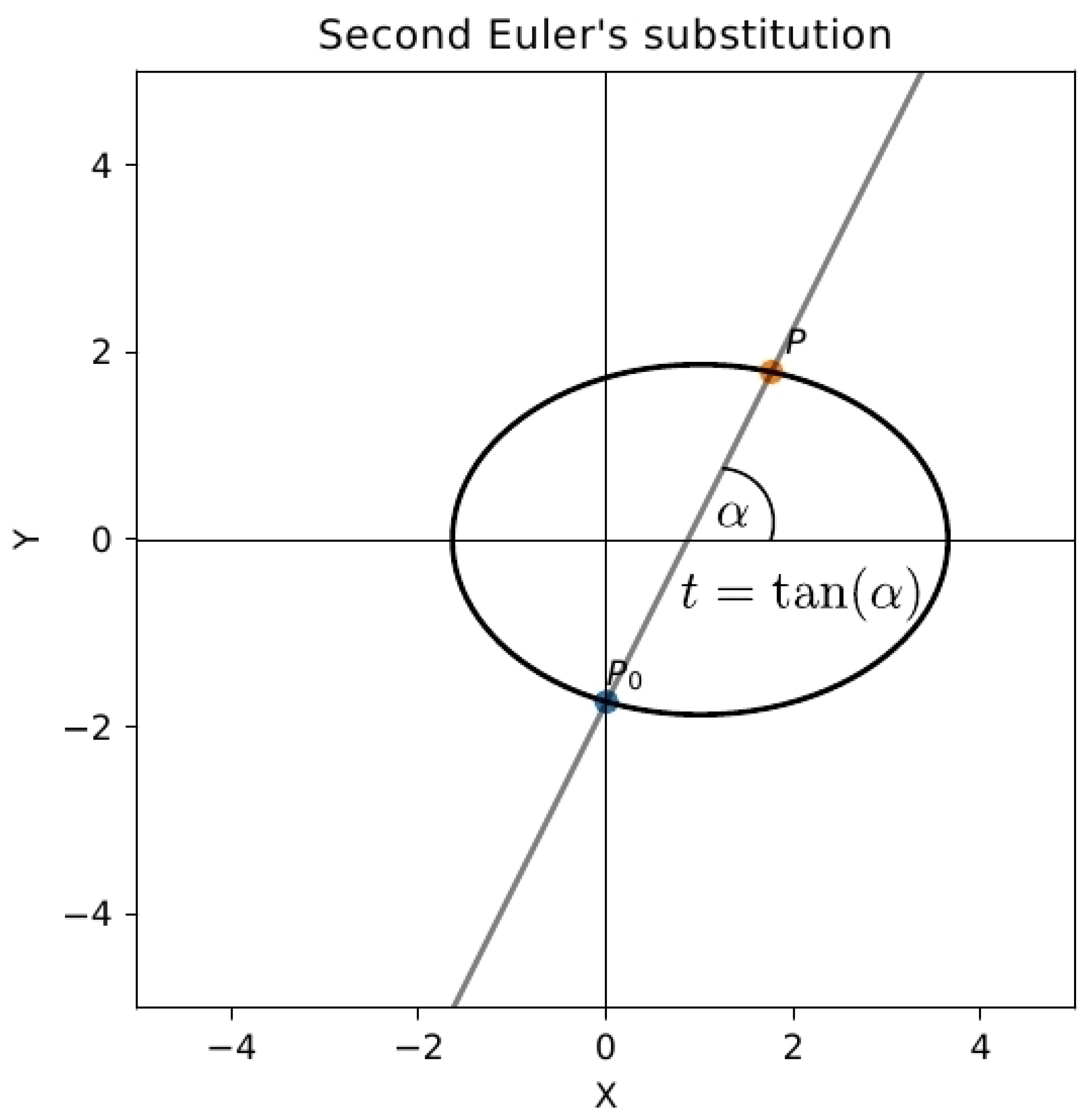
Figure 2.
Geometric interpretation of the second Euler substitution in the case and . The point P is parameterized by the slope t of the line .
Figure 2.
Geometric interpretation of the second Euler substitution in the case and . The point P is parameterized by the slope t of the line .
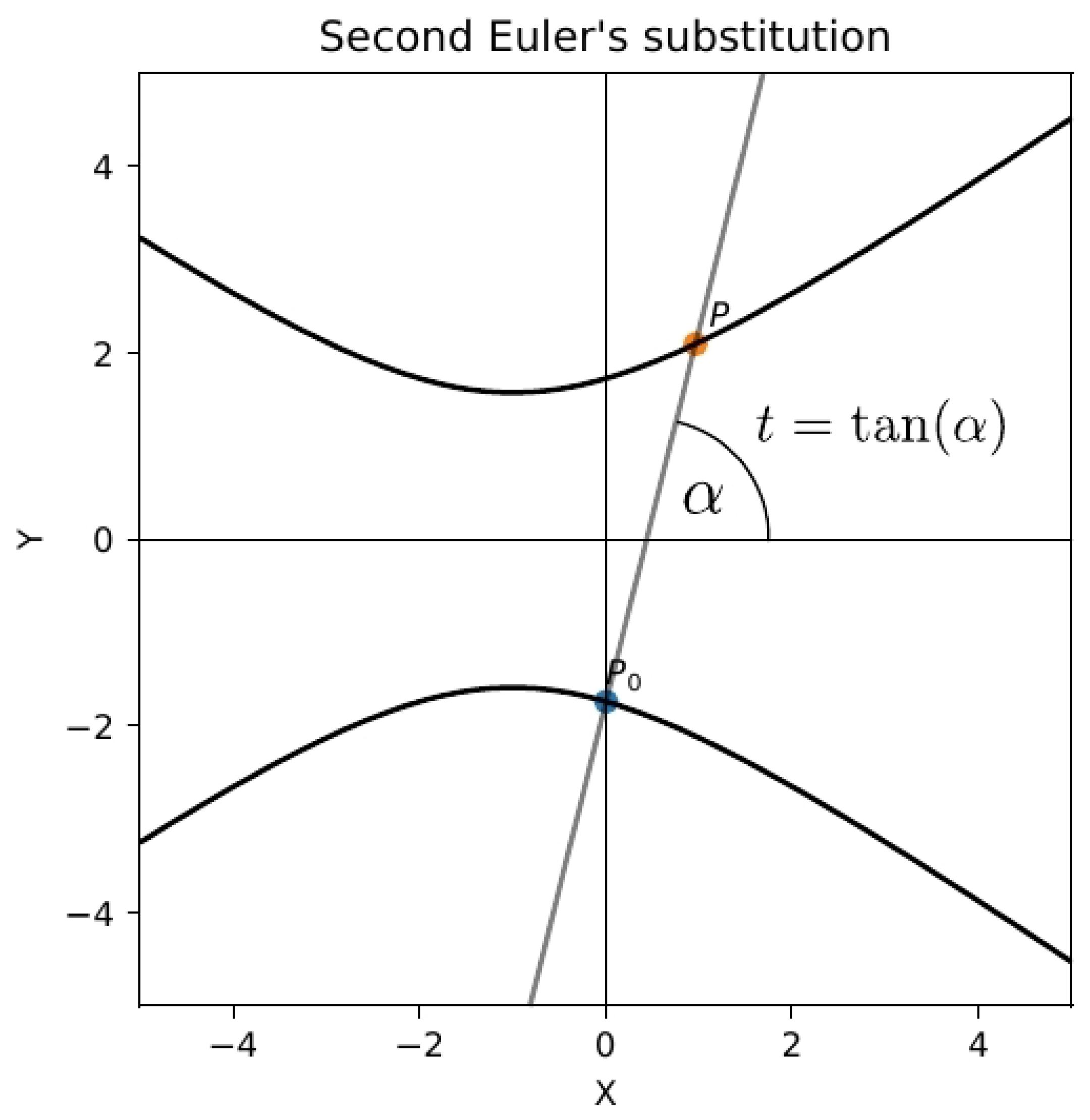
Figure 3.
Geometric interpretation of the third Euler substitution in the case and . The point P is parameterized by the slope t of the line .
Figure 3.
Geometric interpretation of the third Euler substitution in the case and . The point P is parameterized by the slope t of the line .
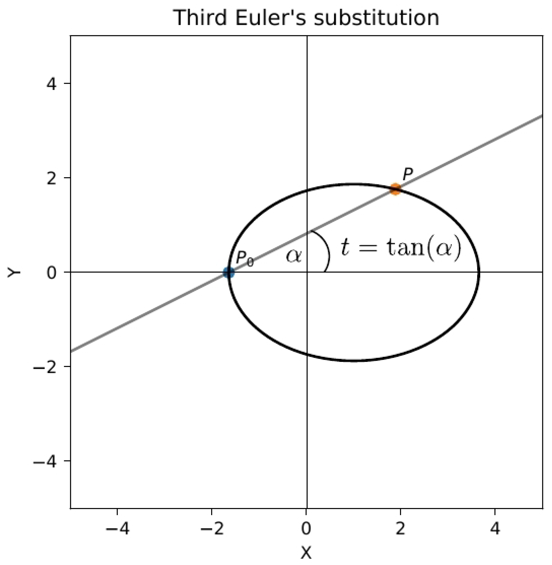
Figure 4.
Geometric interpretation of the third Euler substitution in the case . The point P is parameterized by the slope t of the line .
Figure 4.
Geometric interpretation of the third Euler substitution in the case . The point P is parameterized by the slope t of the line .
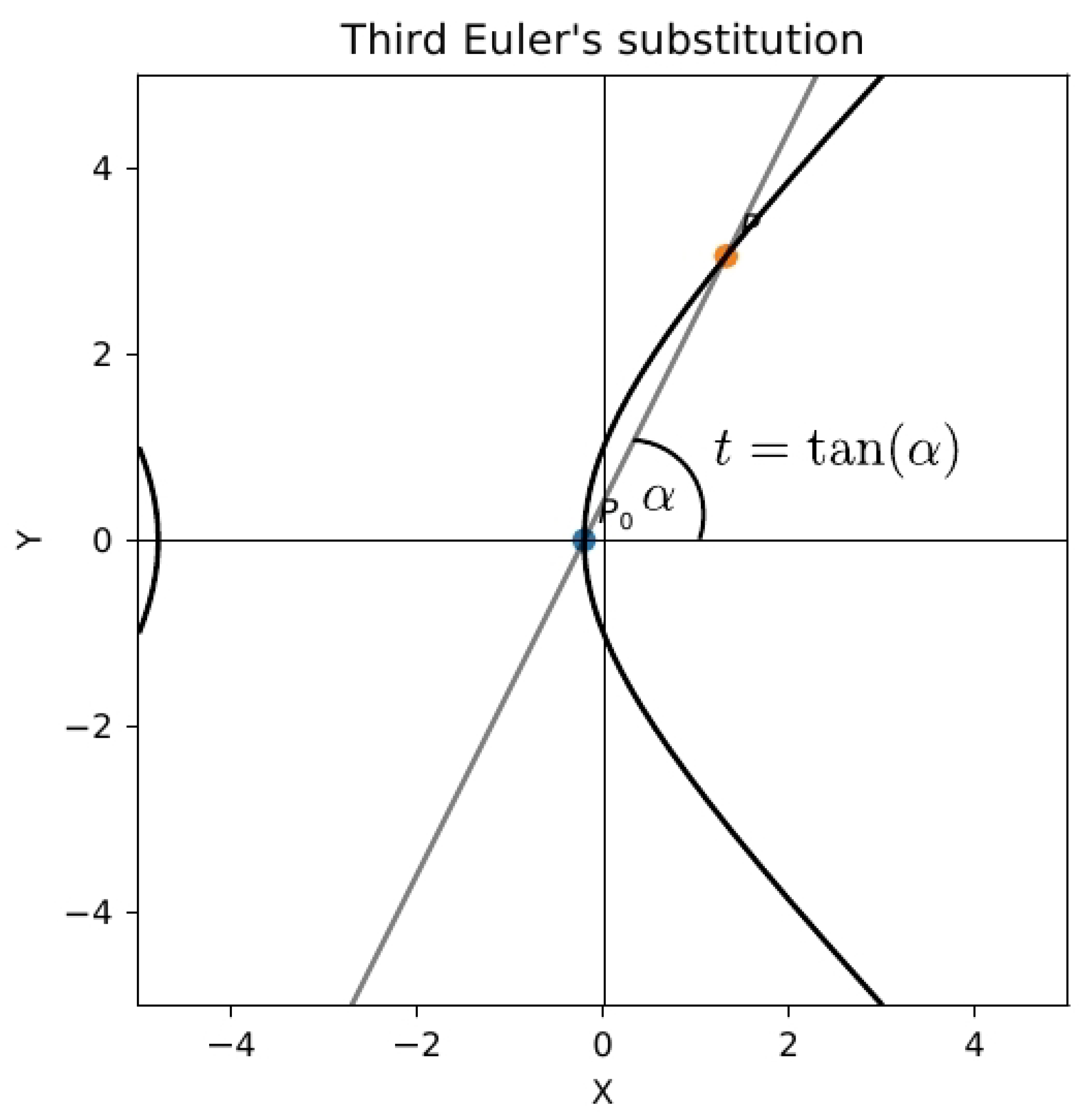
Figure 5.
Geometric interpretation of the first Euler substitution. The points P and are parameterized by intersections t and , respectively, of the y-axis with the line parallel to one of the asymptotes of the hyperbola .
Figure 5.
Geometric interpretation of the first Euler substitution. The points P and are parameterized by intersections t and , respectively, of the y-axis with the line parallel to one of the asymptotes of the hyperbola .
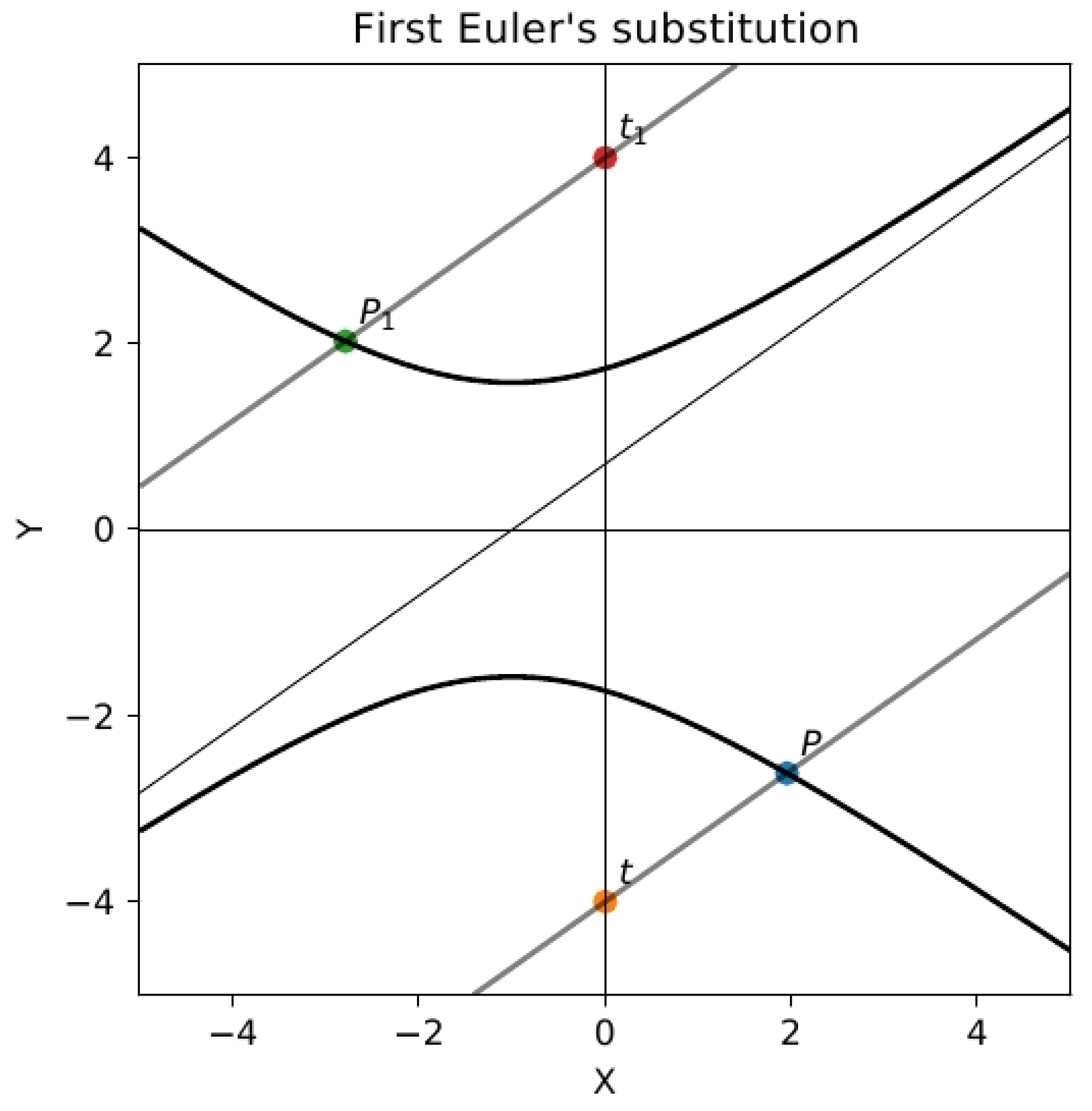
Figure 6.
Characteristic points on the graph of an ellipse: intersections with the coordinate axes (provided that they exist) and extremes (minimum and maximum ).
Figure 6.
Characteristic points on the graph of an ellipse: intersections with the coordinate axes (provided that they exist) and extremes (minimum and maximum ).
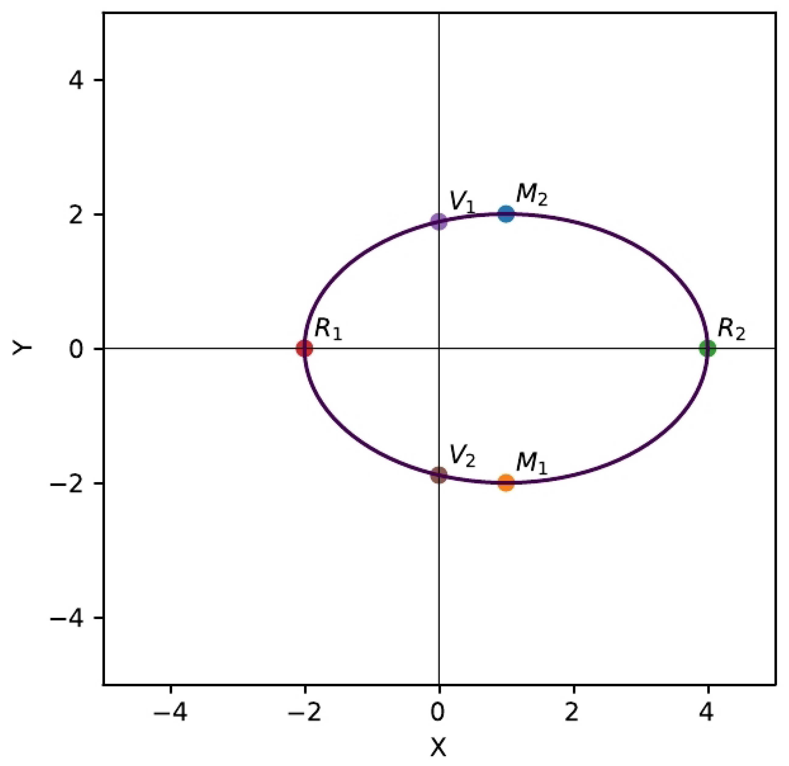
Figure 7.
Characteristic points on the graphs of hyperbolas (two hyperbolas with the same are presented): intersections with the coordinate axes (, , , ) and extremes (, ).
Figure 7.
Characteristic points on the graphs of hyperbolas (two hyperbolas with the same are presented): intersections with the coordinate axes (, , , ) and extremes (, ).
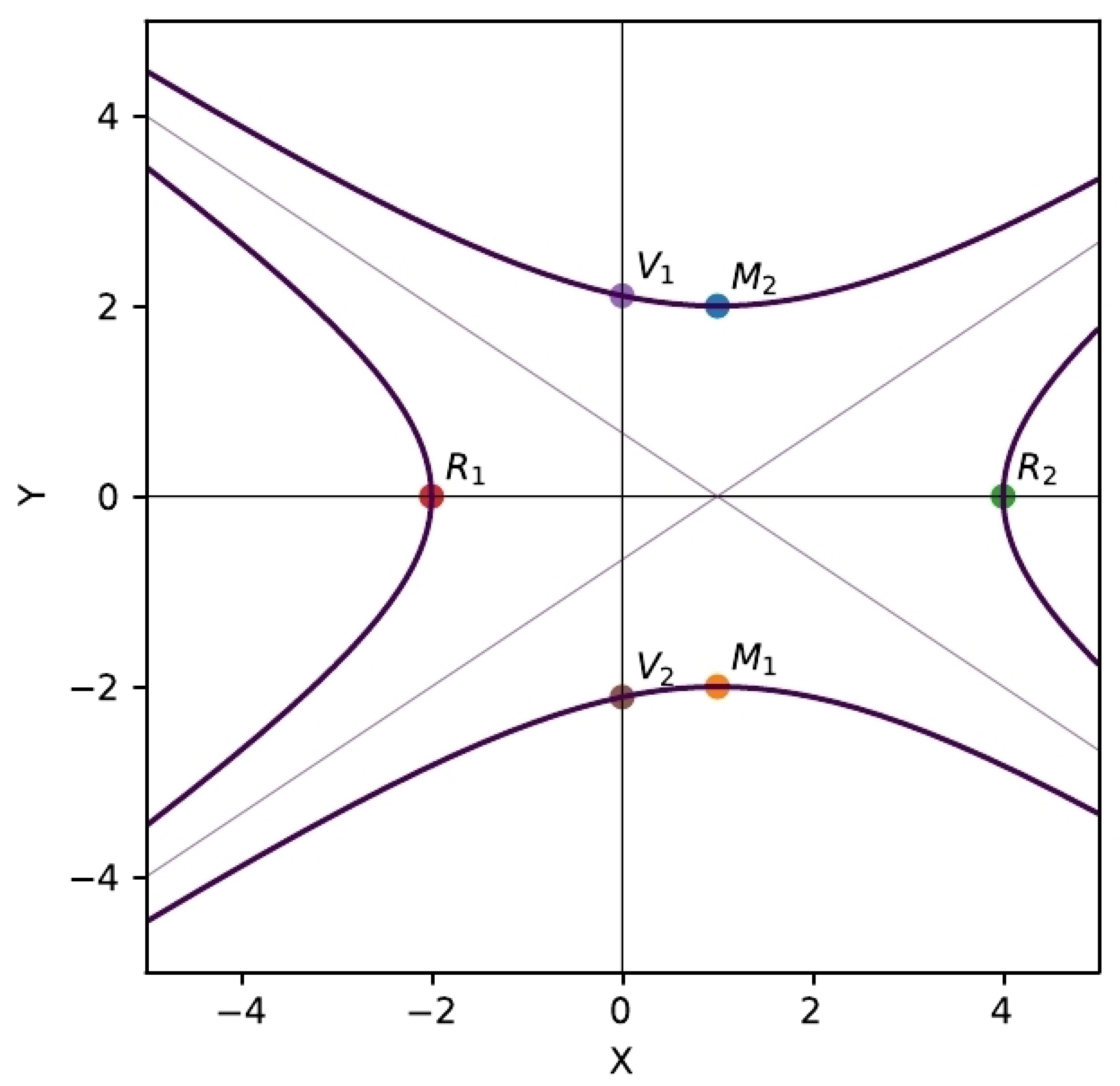
Figure 8.
Geometric interpretation of the fourth Euler substitution in the case . The point P is parameterized by the slope t of the line , where .
Figure 8.
Geometric interpretation of the fourth Euler substitution in the case . The point P is parameterized by the slope t of the line , where .
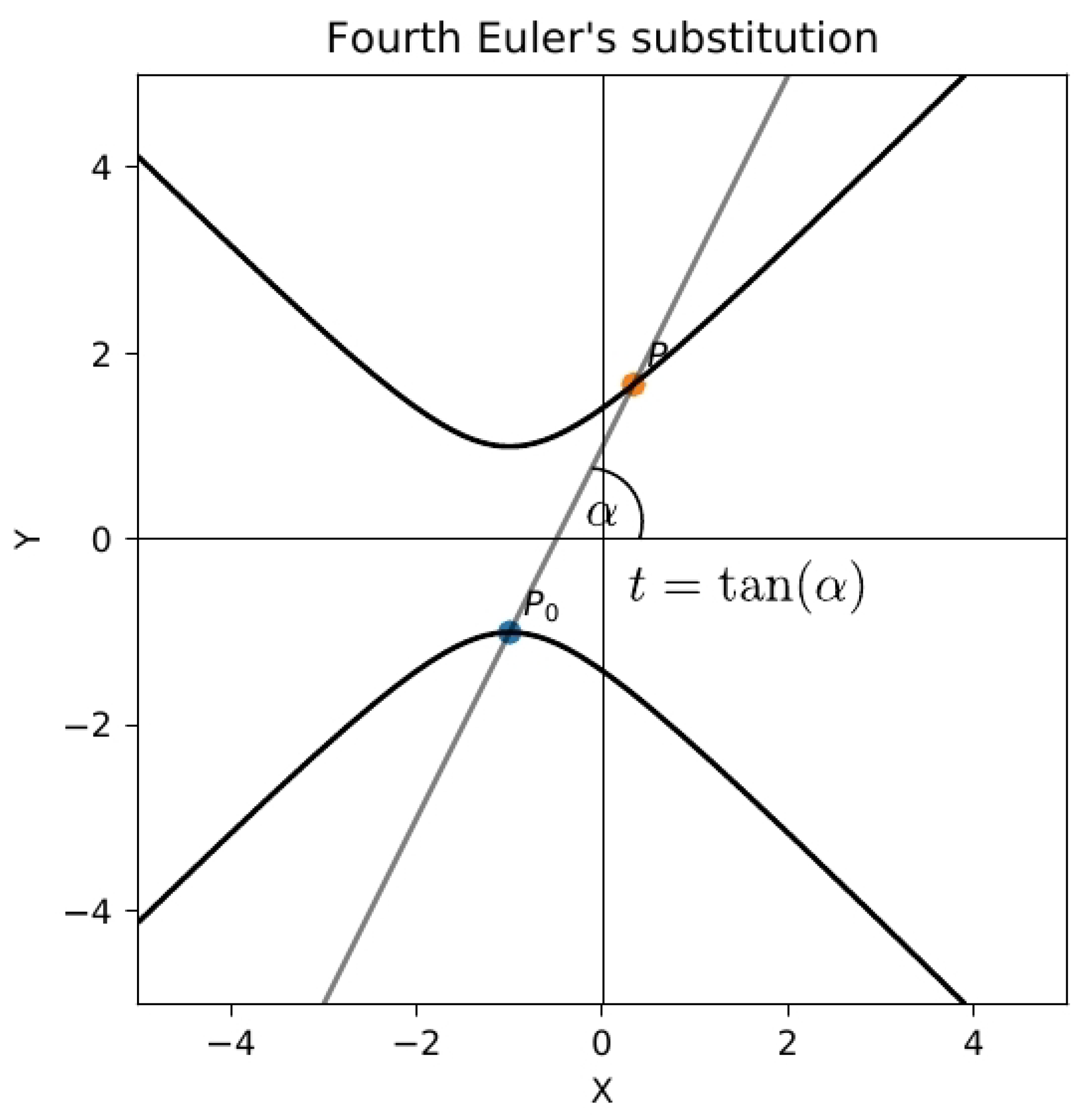
Figure 9.
Geometric interpretation of the fourth Euler substitution in the case . The point P is parameterized by the slope t of the line , where .
Figure 9.
Geometric interpretation of the fourth Euler substitution in the case . The point P is parameterized by the slope t of the line , where .
Disclaimer/Publisher’s Note: The statements, opinions and data contained in all publications are solely those of the individual author(s) and contributor(s) and not of MDPI and/or the editor(s). MDPI and/or the editor(s) disclaim responsibility for any injury to people or property resulting from any ideas, methods, instructions or products referred to in the content. |
© 2023 by the authors. Licensee MDPI, Basel, Switzerland. This article is an open access article distributed under the terms and conditions of the Creative Commons Attribution (CC BY) license (http://creativecommons.org/licenses/by/4.0/).
Copyright: This open access article is published under a Creative Commons CC BY 4.0 license, which permit the free download, distribution, and reuse, provided that the author and preprint are cited in any reuse.


