Submitted:
27 September 2023
Posted:
28 September 2023
You are already at the latest version
Abstract
This paper aims to discuss the relationship between financial development and inflation in Kenya using time series data between 1973 and 2021. The short- and long-run impact of financial development on inflation remains an important issue in the empirical and theoretical literature especially for country specific, but has yet to receive significant research consideration. For this purpose, the paper uses an ARDL analysis method, which is considered an advanced analytical model. Empirical findings confirmed that financial development has a significant long-run impact on inflation in Kenya. On the contrary, results confirmed that there is no significant short-run effect of financial development on inflation. In addition, there is significant long-run and short-run negative relationship between interest rate and inflation. The results indicate significant long-run Granger and ARDL causality from financial development to inflation. The main policy implications of the empirical results of this paper suggest supervision of financial sector must be directed in a way that would stimulate a stable and a moderate inflation rate. In particular, both financial institution and government should enhance the infrastructures of the financial market and promote the utilisation of financial services.
Keywords:
financial development and inflation
; ARDL approach
; causality
; time series
; Kenya
1.0. Introduction
The relationship between financial development and inflation has recently received attention from numerous empirical studies in both developed and developing countries. The thrust of this debate has been whether financial development Granger causes inflation, or whether it is the inflation which Granger causes financial development. Despite the rich body of literature on the impact of financial development on inflation, salient questions remain unanswered. For instance, what is the impact of country-level financial development on inflation, and to what extent does the conditional effect of financial development via inflation and interest rate influence the pace and direction of financial development?. The Figure 1 gives an overview of directional change in the characteristic of Kenya development index from 1980 to 2021.
Kenya’s level of financial development is not too far off from the predicted level and it is considered to have one of the most developed financial systems in Africa (Allen et al. 2012). The country has well developed financial systems that it is Banking, Insurance, Capital Markets, Pension Funds, Savings and Credit Cooperative Societies (SACCOs), Microfinance institutions (MFIs), Building Societies, Development Finance Institutions (DFIs) and informal financial services such as Rotating Savings and Credit Associations (ROSCAs) Popiel, (1994). There are five regulatory bodies that regulate banking, capital markets, insurance, pensions and Savings and Credit Cooperatives (Sacco) sectors, regulated and supervised by the central bank of Kenya(CBK), capital market authority(CMA), insurance regulatory authority (IRA), Retirement Benefits Authority(RBA) and Sacco Societies Regulatory Authority(SASRA), respectively. In Kenya banking sector dominates the financial market, according to bank supervision annual report (CBK 2022), as at December 31, 2022 the sector comprises of 38 banking institution, 37 were privately owned while the Kenya Government had majority ownership in 2 institutions. Of the 37 privately owned banks, 20 were locally owned (the controlling shareholders are domiciled in Kenya) while 17 were foreign owned. The 20 locally owned institutions comprised 19 commercial banks and 1 mortgage finance company. The depth of the Kenya banking system places it ahead of its Sub-Sahara Africa peers (with private credit and domestic deposits at 30.13 percent and 35.92 percent of GDP, respectively). Banks have relatively well-developed branch networks in the country; however, only 84 percent of the population had a bank account in 2022. Likewise, access to credit is challenging for some vulnerable groups and for small- and medium-sized enterprises (SMEs).
Kenya has experienced a rise in inflation owing to various several macroeconomic forces which have been kept at bay by the various interventions of current monetary and the expansionary fiscal policies adopted by the Central Bank (CBK, 2022). The general worst-case effect of inflation would be the failure of a country to meet its financial requirements as and when they fall due, thus exposing the country to harsh financial position in the global economy. This would ultimately make a country less attractive to the desirable international market investments (Gharagozloo, Chen, & Pour, 2022).The effects of inflation on financial sector development has been put at the core of research, particularly after the global economic crises and market crash in 2007, as well as the Covid-19 pandemic (Dumitrescu, Kagitci, & Cepoi, 2022). Kenya, the inflation pressures, nevertheless, seem to be going up in the recent years , pointing to the need for policy makers to keep an eye on inflation changes to ensure that price stability is maintained. A combination of factors notably, rising global crude oil prices caused by Russian Ukraine invasion, drought or erratic weather patterns that adversely impacted agriculture, and weak local currency as a result of weakening in current account deficits, unstable financial sector developments trigger the growing inflation developments.
The average rate of inflation, based on consumer prices (annual %) measurement was approximately 12% during the period between 1973 and 2021. But for the period between 2007 and 2021, the average inflation rate was approximately 8.4%, where the inflation rate in 2008 reached approximately 26.2% compared to 2.0 % in 2002. This rise in inflation rate was attributed to several factors, including both external and internal. As for the external factors: Arab oil embargo in 1973, Iranian revolution energy crisis in 1979, global financial crisis in 2007-2008 and Russia’s war in Ukraine and its impact on the crude oil prices and hence increase the prices of other products. As for the internal factors: early 1990s, shortly before the first multiparty elections, the Treasury created an illusory explosion of wealth in Kenya by printing billions of shillings. The resulting inflation impoverished millions of rural people. The year 2008 to 2011 occasioned by internal shocks (post-elections disruptions, unfavourable weather conditions and high cost of food and fuel prices. It is noted, according to the annual reports of the Central Bank of Kenya for the years 2008 and 2011 that the inflation rates for these years were 26% and 14%, respectively, as they had a role in the decline in growth rates in the volume of credit to private sector. The growth rate in the credit decreased from 25.8% to 2.8% from 2014 to 2018. Therefore without managing inflation rates, it would be difficult for moneylenders to price loans, which would limit credit and investments and as a result it would have a negative impact on the economy.
Even though recent transformations and developments in the financial sector, achieving a balance between financial development and inflation rates is subject that need to be addressed without deviating to the theoretical standpoint of the quantity theory of money that financial development can lead to inflationary pressures (Rousseau & Tarazi, 2002) via the extension of credit and loans, among other causes, in the economy. Huybens and Smith (1999) hypothetically argue that in a steady state with relatively little capital stock in which both banks and stock markets are active, inflation and economic growth must be negatively correlated. This negative connection will become more noticeable at relatively high levels of inflation. To advance the literature of the relationship between financial development and inflation, this research examines the impact of financial development on inflation in Kenya applying ARDL model over the period 1973–2021. This study for that reason aims at contributing to the relationship between inflation and financial development in Kenya.
2.0. Literature review
There is extensive literature on the relationship between financial development and economic growth but a limited empirical research on the relationship between inflation and financial development. However, the relationship between inflation and financial development has been received growing attention in recent years for example Ahmed & Elsayed (2023), Utonga & Ndoweka (2023), Ismail & Masih (2019), Kagochi, (2019), Zermeño et al. (2018) , Ozturk & Karagoz (2012), Bittencourt (2011) and Kim & Lin (2010) studied the interaction between inflation and financial development. The relevance of each study and the selection of indicators are country specific, as countries have different political, legal and institutional frameworks (Lynch, 1996).
As put forward by Ahmed & Elsayed (2023), inflation rate, economic growth, exchange rate, and trade openness jointly impact financial development in the short and long term but is impossible to use the financial development index to predict the inflation rate in Egypt in the short and long term. Utonga & Ndoweka (2023) used VECM analysis method to study the impact of financial development on inflation in Tanzania their study revealed that financial development has a significant long-run impact on inflation in Tanzania, however it had no impact in the short-run. Ismail and Masih (2019) studied the interaction between inflation and financial development in Sudan using the ARDL and nonlinear ARDL algorithms. The empirical study revealed that there was symmetrical long-term equilibrium between inflation and financial development, whereas the short-term relationship was asymmetrical. Kagochi (2019) examined the association between inflation and the performance of the financial sector in sub-Saharan African countries. The study examined panel data and discovered that inflation does not contribute to the development of the region’s financial sector. Zermeño et al. (2018) applied panel quintile regressions to study the relationship between inflation and financial sector performance for 84 countries for the period from 1980 to 2010. The outcomes indicate a steadily negative and nonlinear effect of price increases on financial variables; in specific, it is statistically significant in the full sample of countries, significant in developing nations, and insignificant in advanced nations. Ozturk and Karagoz (2012) examined the relationship between inflation and financial development in Turkey. The findings revealed that inflation has a negative impact on financial development and stressed the unfavourable concerns of high inflation on economic growth. Bittencourt (2011) applied time series data and panel time series data to examine the impact of inflation on financial development in Brazil. Negative effect of inflation on financial sector development is discovered. Kim and Lin (2010) examined the dynamic interaction between inflation and financial development in an empirical study. The paper studied the long-run connection between inflation and financial development for 27 selected countries from 1970 to 2006 using the ARDL model. The empirical study applied causal relationship between the two variables, the Granger causality test and variance decomposition analysis were utilized. The results revealed that financial development had unfavourable long-run impact on inflation. Nevertheless inflation, had a positive effect on financial development, indicating that inflation stimulates the development of the financial sector. Additionally, the empirical study established that financial development triggered inflation rather than the vice versa. The paper also discovered that different countries’ levels of economic and financial development had an effect on the link between inflation and financial development.
On the other hand, and to the best of my knowledge, there is no literature yet that have particularly examined inflation and financial development using ARDL approach in the Kenya context, hence I will give a humble attempt to fill the explained literature gap. Most studies have examined the relationship between financial development and economic growth. Uddin et al (2013) re-examined the relationship between financial development and economic growth in Kenya over the period of 1971–2011 using ARDL bounds testing and Gregory and Hansen's structural break cointegration approaches. The study findings revealed that in the long run, the development of the financial sector has a positive impact on economic growth. Chen et al (2020) examined the asymmetric effects of financial development on economic growth using a model augmented with inflation and government expenditure asymmetries to inform model specification over the period of 1972 to 2017. The authors clearly demonstrate that an environment steered by stable and sustainable inflation that regulated government expenditure and inclusive financial system deepening would positively cause economic growth. Odhiambo (2009), examined the direction of causality between financial development and economic growth in Kenya by examining the impact of inflation on the finance-growth nexus. The empirical results revealed that economic growth Granger-causes financial development in Kenya irrespective of whether the causality is estimated in a bivariate framework or in a trivariate setting. Based on the research gap and contradictory results of these studies, additional research was required to understand the link between financial development and inflation in Kenya.
3.0. Research methodology
3.1. Data source and description
This study uses annual data obtained from the World Bank (World development indicator) covering the period from 1973 to 2021. This period was chosen based on the data availability. The selection of the variables is based on their theoretical and empirical relevance to measure both financial development and inflation in the study’s context. The economic variables used in this study are: inflation rate is measured by the consumer prices (annual %) (INFt), financial development index (FDt) is measured by depth, access, and efficiency and real interest rate (INTt), as a control variable. To avoid the problem of heteroscedasticity, all variables included in this study were transformed to natural logarithms. So, we can specify our long-linear model as follows:
lnINFt = α0 + α1lnFDt + α2lnINTt + μt
Where:
LnINFt: Natural logarithm of inflation rate
lnFDt :Natural logarithm of financial development index
lnINTt :Natural logarithm of real exchange rate
α0,α1 : Coefficients to be estimated
μt : White noise error term
3.2. Econometric Methodology
3.2.1. Test of Unit Root
Economic analysis proposes that there is a long-run relationship between variables and that the means and variances are constant and not dependent on time. In the case of time-series variables, this stationarity of variables is not always satisfied. However, in our study, only the ADF test and PP test were applied to check whether the series was stationary or not. Let us consider the calculation of the following equation by using ADF and PP, developed by Dickey and Fuller (1989) and Phillips–Perron (1988) respectively. The ADF equation is as follows:
3.2.2. ARDL Modeling Specification
To examine the relationship between inflation and financial development, the autoregressive distributed lag (ARDL) bounds testing method suggested by Pesaran et al., (2001) is used. The model is written as follows:
In Equation 4 β0, β1, β2, and β3 show the short-term coefficients; contrary to, and represent the long-term coefficients and error term. In addition, the ECM equation is given below for short-run relationships.
The null hypothesis of nocointegration in the long run relationship is defined by, is tested against the alternative of by means of F-test. However, the asymptotic distribution of this F-statistic is non-standard irrespective of whether the variables are I (0) or I (1).
4.0. Empirical Results and discussion
4.1. Descriptive Statistics
This section shows the descriptive statistics of natural log of inflation (INF), financial development (FD) and interest rate (INT) from 1973 to 2021 as shown in Table 1. The statistics describe the distribution of the variables over time. For inflation, the average inflation rate over the period was 2.28, with a standard deviation of 0.66. This suggests that inflation was highly spread over the period. For financial development the data followed the same trend as of inflation rate with a mean of 3.15 and a standard deviation of 0.21 suggesting this two variable can explain each other. In short descriptive statistics gives us an over view of the behaviour of the variables but it has a limited information about the impact and relationship among the variables.
4.2. Correlation Analysis
The paper used the Pearson correlation coefficient to determine the strength and direction of the linear association between INF, FD, and INT (Pearson, 1896). For inflation and financial development which indicates -0.4732 that is they’re negatively correlated. In other words, when INF increases, FD tended to decrease as well and vice versa. Inflation and interest rate are inversely correlated that confirms the theory between the two variables. For financial development and interest rate which indicates 0.3018 are positively correlated. The Table 2 shows the correlation matrix computation.
4.3. Unit root test
To progress further, it’s essential to check the stationarity for each variable included in this study. Hence, unit root test needs to be applied to check for stationarity. The augmented Dickey-Fuller AD-F) and Phillips-Perron (PP) unit root tests were applied; the results are presented in (Table 3). Results show that inflation is stationary in its level but financial development and interest rate they are stationary in first difference, which means the variables are combination of integrated level, or I (0) and integrated of order one, or I (1) . Since, the results show that the variables are not integrated of order greater than one and are combination of orders, and our sample size is small, therefore we should adopt ARDL approach to test for long run relationship between the variables by applying ARDL cointegration test.
4.4. Optimum lag Selection Criteria
The selection of optimal lag length of the variables of interest is important in econometric model estimation. This is important in order to avoid spurious rejection or acceptance of estimated results. There are Likelihood Ratio (LR), Forecast Prediction Error (FPE) Criteria, Akaike Information Criteria (AIC), Hannan Quinn Information Criteria (HQIC), and Schwartz Bayesian Information Criteria (SBIC). In the case of conflicting results, CEPR (2001) suggested following the SBIC for any sample size for the quarter and annual data (Ivanov & Kilian, 2001). The selection of the lags order in ARDL model was based in the minimum value of SBIC. Below is lag length criteria table: Therefore, based on lag length criteria lag 1 is the best lag length for this analysis and Schwarz Information Criterion is the best criterion for this study. After the selection of the lag length, the ARDL bound test for Co-integration follows:

Table 4.
Results of Optimal lags.
| Lag | LL | LR | df | P | FPE | AIC | HQIC | SBIC |
| 0 | -44.4306 | .006737 | 3.51338 | 3.55619 | 3.65736 | |||
| 1 | -2.25566 | 84.35 | 9 | 0.000 | .000581 | 1.05597 | 1.22723* | 1.6319* |
| 2 | 8.04222 | 20.596* | 9 | 0.015 | .000544* | .959836* | 1.25953 | 1.96771 |
| 3 | 15.4532 | 14.822 | 9 | 0.096 | .000659 | 1.07754 | 1.50567 | 2.51736 |
| 4 | 19.0519 | 7.1973 | 9 | 0.617 | .001141 | 1.47764 | 2.03421 | 3.3494 |
Source: Authors’ calculation using Stata 14.
4.5. The Bounds Test Results
The Bound testing cointegration result is presented in Table 5. According to Pesaran et al., (2001), the computed F-Statistic should be compared with lower bound and upper bound value at chosen significant level. From the empirically obtained results, the computed F-Statistic which is 10.859, is more than the upper bound value (6.36) at 1% significant level. Hence, the null hypothesis of no cointegration is rejected. The study concludes that there exists a long run relationship between the variables under consideration
4.6. ARDL Long-Run Results
Equation (6) presents the results of the long-run relationship between the variables. The results show that there is significant and negative long-run relationship between financial development and inflation. A percentage change in financial development is associate with 1.22 % decline in inflation on average ceteris paribus at 5% level. The results also show that there is significant long-run negative relationship between interest rate and inflation. A percentage change in interest rate is associate with 0.38 % decline in inflation on average ceteris paribus at 5% level. The existence of a long-run relationship between inflation and financial development is consistent with majority of empirical studies (Gao et al., 2012, Kim and Lin 2010, Akinkoye et al., 2015; Lee and Wong, 2005).The negative relationship between inflation and interest rate in Kenya is consistent with the conventional view of economists. That is the higher the interest rate the lower the inflation. In the Table 6 R square value indicated that 47.5% in inflation is due to all predictors used in the study and 52.5% is explained outside the model.
lnINF= 5.94 -1.22lnFD - 0.38lnINT
The coefficient of Error correction term gives the speed of the short-run adjustment. Its negative and significant, implying model convergence in the long run between dependent and independent variables. The error correction term (-0.8726), confirms that all the variables are cointegrated or have long-run relationships. This finding supports other empirical studies in the literature (Hassan and Bashir, 2003; Al-Awad and Harb, 2005; Chuah and Thai, 2004; Gao et al., 2012).Any deviations from the long-run equilibrium are corrected at an adjustment speed of 87.26%.
4.7. ARDL Short-Run Results
The results of the ARDL short run model indicate that interest rate is negatively correlated with inflation in the short run. In addition, a 1% change in interest rate will change inflation by 33.6% and vice versa. Furthermore, the findings postulated no significant relationship between financial development and inflation in the short run. In addition, the 34.28% variations in the inflation are due to all the predictors used and 65.72% are outside the model. These relationships are shown in Table 7.
4.8. Granger causality test
From Table 8 shows the result of the Granger causality test. The results show that there exists a unidirectional causality from interest rate to inflation. Also, a unidirectional causality runs from interest rate to financial development.
4.9. ARDL Causality
From Table 6, the error correction term is negative (-0.8726) and significant at the 1% level (p = 0.000). This implies that there is a significant long-run causality running from financial development to inflation. Additionally there was long run causality running from interest rate to inflation. According to Table 9, there was short run causality running from interest rate to inflation but there was no short-run causality flowing from financial development to inflation. Thus, the 5% p-value indicates that there was only short term causality between interest rate and inflation but no short-term causality between financial development and inflation.
4.10. Diagnostic test
Table 10.
Diagnostic statistics tests.
| Diagnostic Statistics Tests | p-Values | Results |
| Breusch Godfrey LM | 0.9800 | No serial correlations problem |
| Breusch-Pagan-Godfrey | 0.3079 | No heteroscedasticity problem |
| Heterogeneity | 0.7446 | No heterogeneity Problem |
Source: Authors’ calculation using Stata 14.
Several diagnostic tests were performed to ascertain the validity and accuracy of the inflation model results. The Breusch and Pagan (1979) heteroskedasticity test revealed that the model was homoscedastic (0.3079>0.05). The optimal lags adopted by Schwartz Bayesian Information Criteria (SBIC) automatic lag selection were 1, 0, and 0. The Breusch and Godfrey (1978) LM autocorrelation test was employed with the results revealing that the error terms were not serially correlated (0.9800>0.05).
5.0. Conclusion
This study mainly focused on evaluating the impact of financial development on inflation in Kenya, using a new applied technique. Many previous theoretical and applied studies dealt with the role of the financial development and its impact on economic growth in Kenya. Some studies elsewhere have found that the impact of financial development on inflation is negative when inflation rates reach certain levels. Some studies also were consistent with this finding of impact of financial development on inflation but they utilized a different approach.
The study utilised time-series data from 1973 to 2021. The financial development was used as a proxy for domestic credit to private sector(%GDP) and its more relevant in developing countries in which most financial development occurs within the banking system (Keho, 2009).The inflation rate was used as a proxy for inflation, consumer prices (annual %). The interest rate was used as a proxy for real interest rate (%) The data were sourced from the World development indicator. The study employed the ADRL model analysis technique and Granger causality test to examine the direction of the causality between the variables.
The results of this study observed that financial development has a significant long-run impact on inflation in Kenya. There was a unidirectional causality running from financial development to inflation. The short-run estimates reveal that financial development has no significant effect on inflation and had no short-run causality flowing from financial development to inflation. This implies that financial development is a reliable strategy for controlling inflation in the long run. The results also show that there is significant long-run and short-run negative relationship between interest rate and inflation. Additionally there was long run and short run unidirectional causality running from interest rate to inflation.
The major recommendation from these findings is that supervision of financial sector must be directed in a way that would stimulate a stable and a moderate inflation rate. It is imperative that the government implement suitable regulatory policies and exercise oversight over financial institutions and proficiently administering interest rates that are suitable for the country. The study concludes that both financial institution and government should enhance the infrastructure of the financial market and promote the utilisation of financial services. Enhancing the scope of financial institutions and augmenting credit accessibility can result in strengthened financial inclusion, higher investment, and economic growth and this will hinder against inflationary forces and unwarranted credit expansion.
Disclosure statement
No potential conflict of interest was reported by the authors.
Funding
No funding sources were provided for this paper.
References
- Ahmed, M. M. Ahmed, M. M., & Elsayed, A. E. (2023). The Relationship between Financial Development and Inflation Rate in Egypt. Indian Journal of Economics and Development,.
- Akinkoye E; the case of Nigeria: Y., Sanusi K.A., Moses P.O., 2015, Dynamic interaction between inflation and credit rationing.
- Al-Awad M., Harb N., 2005, Financial development and economic growth in the Middle East, “Applied Financial Economics”, 15(15).
- Allen, F., Carletti, E., Cull, R., Qian, J., Senbet, L. and Valenzuela, P. (2012), “Resolving the African financial development gap: cross-country comparisons and a within-country study of Kenya”, NBER Working Paper No. 18013, Cambridge, MA.
- Bittencourt, M; evidence from Brazil: (2011). Inflation and financial development.
- Breusch, T; "Testing for Autocorrelation in Dynamic Linear Models: S. (1978).
- Breusch, T; Journal of the econometric society: S., & Pagan, A. R. (1979). A simple test for heteroscedasticity and random coefficient variation. Econometrica.
- CBK; //www.centralbank.go.ke/uploads/banking_sector_annual_reports/1376276635_2022%20Annual%20Report: (2022). Publication Central bank of Kenya bank supervision annual report, 2022. Nairobi.https.
- Chen, H; evidence from NARDL: , Hongo, D. O., Ssali, M. W., Nyaranga, M. S., & Nderitu, C. W. (2020). The asymmetric influence of financial development on economic growth in Kenya.
- Chuah H; Evidence from causality tests for the GCC countries: , Thai W., 2004, Financial development and economic growth.
- Dickey, D. A. Dickey, D. A., & Fuller, W. A. (1979). Distribution of the estimators for autoregressive time series with a unit root. Journal of the American statistical association.
- Dickey, D. , and Fuller, W., (1981): “The Likelihood Ratio Statistics for Autoregressive Time Series with a Unit Root,” Econometrica, 49, 1057–1072.
- Dumitrescu, B. A. Dumitrescu, B. A., Kagitci, M., & Cepoi, C. O. (2022). Nonlinear effects of public debt on inflation. Does the size of the shadow economy matter? Finance Research Letters.
- Gao Q; with an application to evaluate credit rationing in U: , Gu, J., Hernandez-Verme P., 2012, A semi parametric time trend varying coefficients model.
- Gharagozloo, M. M. Gharagozloo, M. M., Chen, C., & Pour, F. S. (2022). The effect of change readiness of economies on international M&A flows. Review of International Business, 32(4), 457-483.
- Hassan M.K., Bashir A.H.M., 2003, Determinants of Islamic banking profitability, ERF annual conference, 10.
- Huybens, E. Huybens, E. and Smith, B. (1999) Inflation, Financial Markets and Long-Run Real Activity. Journal of Monetary Economics, 43, 283-315.
- Ismail, Y. Ismail, Y., & Masih, M. (2019). Is the relationship between inflation and financial development symmetric or asymmetric? New evidence from Sudan based on NARDL. Munich Personal RePEc Archive.
- Ivanov, V. Ivanov, V., & Kilian, L. (2001). A practitioner's guide to lag-order selection for vector autoregressions (CEPR Discussion Paper No. 2685). C.E.P.R.
- Kagochi, J. Kagochi, J. (2019). Inflation and financial sector development in Sub-Saharan African countries. Journal of Economic Studies, 46.
- Keho Y; cointegration and causality analysis for the UEMOA countries: , 2009, Inflation and financial development.
- Kim, D. Kim, D., & Lin, S. (2010). Dynamic relationship between inflation and financial development. Macroeconomic Dynamics, 14.
- Kwiatkowski, D. Kwiatkowski, D. and Phillips, P. and Schmidt, P. and Shin, Y. (1992) Testing the null hypothesis of stationarity against the alternative of a unit root, Journal of Econometrics, 54, pp.159-178.
- Lee C; evidence from Taiwan and Japan: , Wong S.Y., 2005, Inflationary threshold effects in the relationship between financial development and economic growth.
- Odhiambo, N; An empirical investigation: M. (2009a). Finance-growth nexus and inflation dynamics in Kenya.
- Ozturk, N; Evidence from Turkey: , & Karagoz, K. (2012). Relationship between inflation and financial development.
- Pearson, K. Pearson, K. (1896). VII. Mathematical contributions to the theory of evolution.—III. Regression, heredity, and panmixia. Philosophical Transactions of the Royal Society of London. Series A, containing papers of a mathematical or physical character.
- Popiel, P; A comparative study: A. (1994). Financial systems in Sub-Saharan Africa.
- Rousseau, P. L. Rousseau, P. L., & Tarazi, A. (2002). Inflation thresholds and the finance–growth nexus. Journal of International Money and Finance, 21.
- Tinoco Zermeño, M; New evidence from panel quantile regressions: Á., Venegas Martínez, F., & Torres Preciado, V. H. (2018). Effects of inflation on financial sector performance.
- Uddin, G. S. Uddin, G. S., Sjö, B., & Shahbaz, M. (2013). The causal nexus between financial development and economic growth in Kenya. Economic Modelling.
- Uddin, G. S. Uddin, G. S., Sjö, B., & Shahbaz, M. (2013). The causal nexus between financial development and economic growth in Kenya. Economic Modelling.
- Utonga, D; Empirical Evidence from the VECM Approach: , & Ndoweka, B. N. (2023). The Impact of Financial Development on Inflation in Tanzania.
Figure 1.
Financial Development index through Time. Source: IMF. Note: FD, FI and FM denotes financial development, financial institution and financial market, respectively. FID, FIA, FIE, FMD, FMA, and FME, with the letters D, A, and E denoting depth, access, and efficiency, respectively, and I and M denoting institutions and markets, respectively.
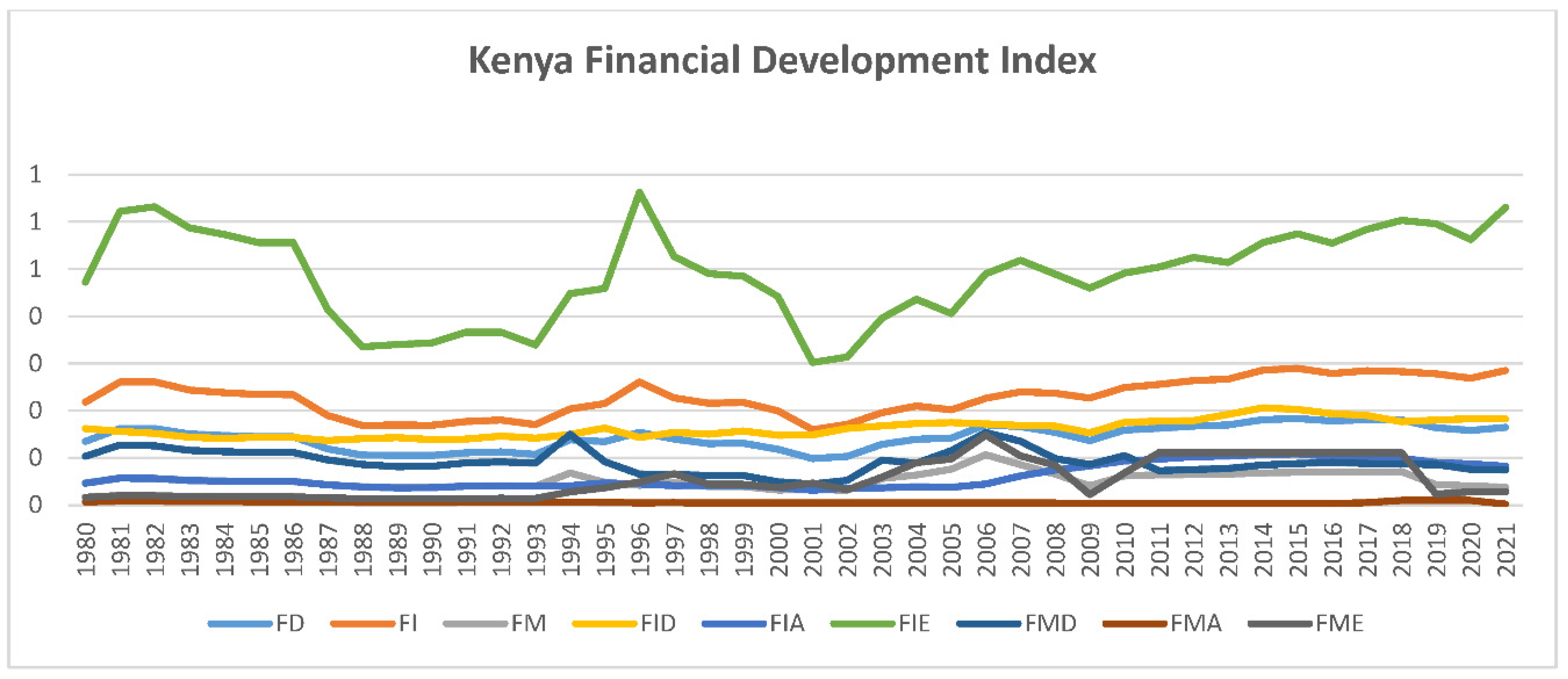
Table 1.
Descriptive statistics for different variables.
| lnINF | lnFD | lnINT | |
| Mean | 2.275443 | 3.149576 | 1.923736 |
| Maximum | 3.828182 | 3.602758 | 3.049099 |
| Median | 2.300586 | 3.130626 | 1.998779 |
| Minimum | 0.4410434 | 2.82299 | -0.0591247 |
| Std. Dev. | 0.6581875 | 0.2098585 | 0.7001613 |
| Skewness | -0.4369283 | 0.4188327 | 3.56648 |
| Kurtosis | 3.779875 | 2.216245 | -0 .6998455 |
| Sum | 111.4967 | 154.3292 | 76.94945 |
| Sum sq. dev | 20.7941161 | 2.11394845 | 19.1188072 |
| Jarque-Bera | 0.2465 | 0.261 | 0.1496 |
| Observations | 49 | 49 | 40 |
Source: Authors’ calculation using Stata 14.
Table 2.
Correlation matrix.
| Variables | lnINF | lnFD | lnINT |
| lnINF | 1.000 | ||
| lnFD | -0.4732 | 1.000 | |
| lnINT | -0.4566 | 0.3018 | 1.000 |
Source: Authors’ calculation using Stata 14.
Table 3.
Results of Unit Root Tests.
| Variables | ADF test | PP test | |||||||
| Level | Difference | Level | Difference | Stationary order | |||||
| Constant | Constant & trend | Constant | Constant & trend | Constant | Constant & trend | Constant | Constant & trend | ||
| lnINF | -3.988 ** | -4.686 ** | - | - | -5.005 ** | -5.662 ** | - | - | I(0) |
| lnFD | -1.157 | -2.921 | -6.596 ** | -6.515** | -1.248 | -3.461* | -8.556** | -8.451 ** | I(1) |
| lnINT | -3.988** | -4.686** | - | - | -2.559 | -2.848 | -6.269 ** | -6.153** | I(1) |
Source: Authors’ calculation using Stata 14. Notes: *, ** & *** indicate 10%, 5%, and 1% significance levels, respectively.
Table 5.
Results of bound test.
| Test Statistic | Value | K |
| F-statistic | 10.859 | 2 |
| Critical Value Bounds | I(0) Bound | I(1) Bound |
| Significance | ||
| 10% | 3.17 | 4.14 |
| 5% | 3.79 | 4.85 |
| 2.5% | 4.41 | 5.52 |
| 1% | 5.15 | 6.36 |
Source: Authors’ calculation using Stata 14. Note: The variables' lag length (1 0 0). H0 (no cointegration) is accepted if F < critical value for I (0) regressors (Lower band); and rejected if F > critical value for I(1) regressors (Upper band).
Table 6.
Results of Long- run analysis.
| Regressor | Coefficient | St. Error | t Value | Prob |
| Error Correction Term (ECT) | -0.8725792 | 0.167206 | -5.22 | 0.000 |
| InFD | -1.215354 | 0.5476702 | -2.22 | 0.033 |
| InINT | -0.3848768 | 0.1738819 | -2.21 | 0.033 |
| Constant | 5.935698 | 1.856666 | 3.20 | 0.003 |
| R squared= 0.4750 Adj squared= 0.4313 |
||||
Source: Authors’ calculation using Stata 14.
Table 7.
Results of short- run analysis.
| Variables | Coefficient | St. Error | t Value | Prob |
| LnINF(-1) | 0.1274208 | 0.167206 | 0.76 | 0.451 |
| LnFD | -1.060492 | 0.5323704 | -1.99 | 0.054 |
| LnINT | -0.335835 | 0.1390083 | -2.42 | 0.021 |
| Constant | 5.935698 | 1.856666 | 3.20 | 0.003 |
| F(3, 36)= 6.26 Prob > F= 0.0016 R squared=0.3428VAdj R-squared=0.2880 |
||||
Source: Authors’ calculation using Stata 14.
Table 8.
Granger causality test results.
| Valiables | Null Hypothesis | Chi-Sq | Prob | Decision |
| InINF | lnFD does not Granger Cause lnINF | 2.3186 | 0.128 | No causality |
| lnINT does not Granger Cause lnINF | 8.4631 | 0.004 | lnINT Granger Cause lnINF | |
| lnFD | lnINF does not Granger Cause lnFD | 1.1693 | 0.280 | No causality |
| lnINT does not Granger Cause lnFD | 13.024 | 0.000 | lnINT Granger Cause lnFD | |
| lnINT | lnINF does not Granger Cause lnINT | 2.7226 | 0.099 | No causality |
| lnFD does not Granger Cause lnINT | 1.2583 | 0.262 | No causality |
Source: Authors’ calculation using Stata 14. Note: The rejection of null hypothesis is at 5 percent level of significance.
Table 9.
t-statistics test results for short-run and long-run causality analysis.
| Variable | Short-run | P-value | Long-run | p-value |
| lnFD | -1.06 | 0.054 | -1.22 | 0.033 |
| lnINT | -0.34 | 0.021 | -0.38 | 0.033 |
Source: Authors’ calculation using Stata 14. Note: The rejection of null hypothesis is at 5 percent level of significance.
Disclaimer/Publisher’s Note: The statements, opinions and data contained in all publications are solely those of the individual author(s) and contributor(s) and not of MDPI and/or the editor(s). MDPI and/or the editor(s) disclaim responsibility for any injury to people or property resulting from any ideas, methods, instructions or products referred to in the content. |
© 2023 by the authors. Licensee MDPI, Basel, Switzerland. This article is an open access article distributed under the terms and conditions of the Creative Commons Attribution (CC BY) license (http://creativecommons.org/licenses/by/4.0/).
Copyright: This open access article is published under a Creative Commons CC BY 4.0 license, which permit the free download, distribution, and reuse, provided that the author and preprint are cited in any reuse.


