1. Introduction

2. Methods

2.2. Numerical Simulation Ensemble Setup

An ensemble of 50 simulations was performed with SPINS which allows for direct numerical simulations (DNS) of the incompressible Navier-Stokes equations. The model uses third-order accurate, variable time step Adams-Bashforth time-stepping and has spectral accuracy in space. When compared to lower order finite difference or volume schemes with the same resolution, numerical errors are much smaller[52]. Further, the numerical dispersion and diffusion errors often found in classical lower order methods are absent from spectral methods. The SPINS code has been extensively validated against linear theory (e.g., growth rate for shear instability and internal wave generation[49]), existing numerical methods (e.g., in the context of dipole–wall collisions[49]), exact solutions (e.g., for the propagation of exact internal solitary waves[53]), and experimental data (e.g., cross-boundary layer transport due to shoaling mode 2 internal waves[54]).

Simulation parameters and dimensionless numbers are given in Table 1. All simulations were run in 2D with a 2.048m wide and 0.512m tall domain. We used 4096 grid points in the horizontal and 1024 in the vertical to have 0.5mm resolution in both directions. Periodic boundary conditions were implemented in x and free slip boundary conditions were implemented in z.

To induce the formation of Rayleigh-Taylor (RT) instabilities, each ensemble member is initialized with an unstable density stratification of the form

$$\begin{array}{cc}\hfill \rho (\overrightarrow{x},t=0)& =-5\times {10}^{-4}\left(1-tanh\left(\frac{z-0.256-\epsilon \left(x\right)}{0.02}\right)\right),\hfill \end{array}$$

(15)

$$\begin{array}{cc}\hfill \epsilon \left(x\right)& =2.5\times {10}^{-3}\sum _{i=1}^4{Y}_{1i}sin\left(\frac{16\pi (Y_{2i}+1)}{2.048}x+2\pi Y_{3i}\right),\hfill \end{array}$$

(16)

where $Y_{ji}\sim U(0,1)$ is a random variable chosen from a uniform distribution between 0 and 1. The distribution is seeded by the start time of each simulation. The only difference between ensemble members is the perturbation, $\epsilon$, applied to the initial density stratification. Panel (a) of Figure 1 shows an example stratification from a subdomain of one of the simulations.

Estimates of the dimensionless numbers were calculated using the domain height as the characteristic length scale and the maximum root-mean-square vertical velocity of a sample ensemble member as the velocity scale. Values are given in Table 1. The Reynolds number, $Re=UL/\nu$, represents the ratio of the inertial to viscous forces. Our simulations have $Re\approx 1.1264\times {10}^4$ indicating the flow becomes turbulent. The Schmidt number, $Sc=\nu /\kappa =7.1429$, tells us the momentum diffusivity is greater than that of the tracers. The Péclet number describes the ratio of advective to diffusive transport and is given by $Pe=Sc·Re\approx 8.0457\times {10}^4$.

In each of the simulations, the reaction term is

$$\begin{array}{c}\hfill F\left(\theta \right)=0.1·\theta (1-\theta )·tanh(\theta /0.001),\end{array}$$

(17)

where the multiplication by the hyperbolic tangent ensures that any oscillations around the unstable equilibrium $\theta =0$ are suppressed. The reaction timescale parameter $\alpha =0.1$ was chosen so that the Damköhler number, which we define as $Da=\frac{\alpha L}{U}\approx 2.3273$, is $O\left(1\right)$. The order of $Da$ was chosen to balance the reaction and advective timescales for the purposes of illustration. A fast reaction (eg. $\alpha =1$) has $\theta \to 1$ too quickly for structures created from turbulent mixing to be observed. Slow reactions (eg. $\alpha =0.01$) allow for the creation of sharp fronts which can be difficult to resolve.

The initial distributions of both the reactive and passive tracers are given by

$$\begin{array}{cc}\hfill {\theta }_0& =0.5\left(1+tanh\left(\frac{z-0.48}{0.06}\right)\right),\hfill \end{array}$$

(18)

so that the tracers lie in a band along the top of the domain as shown in panel (b) of Figure 1. Each simulation evolves both tracers with the same velocity fields and the tracers do not interact. The simulations are stopped after 40s when the system has reached a well-mixed state.

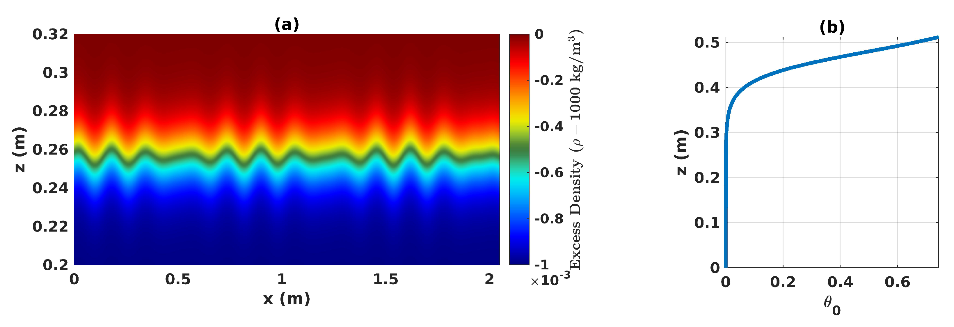
Figure 1. (a) Subdomain with sample initial density stratification perturbed by $\epsilon$ (equation 15). (b) Initial tracer concentration as a function of depth.

Figure 1. (a) Subdomain with sample initial density stratification perturbed by $\epsilon$ (equation 15). (b) Initial tracer concentration as a function of depth.

3. Results

3.1. Tracer Mean and Scalar Variance

The reactive and passive tracers start in a band along the top of the domain with concentration decreasing downwards. Initially, the system is at rest to mimic the accumulation of a tracer in calm waters. If the system started out turbulent, we would expect the tracer to be well-mixed and since turbulent mixing is inherently unpredictable, it would be challenging to draw clear comparisons between the spatial distributions of the reactive and passive tracers. The initial density stratification is centred at $z=0.256$m, about 0.16m below the bottom of the tracer band, meaning there is a delay between the start of the simulation and the time at which the RT instabilities start advecting the tracers. During this time, the tracers begin diffusing downwards and the reactive tracer grows according to the function in equation 17. The reaction both increases the concentration of the tracer and accelerates the downwards spread by enhancing Fickian diffusion. Therefore, the reactive tracer front lies lower in the domain allowing the RT plumes to reach it earlier than the passive tracer.

Figure 2 (stills taken from supplementary movies S1 and S2) shows the (a) mean and (b) scalar variance of the reactive tracer at $t=26$s. When comparing these quantities with those of the passive tracer, panels (b) and (d), it is clear that the mean concentration of the reactive tracer is nearly twice that of the passive tracer and extends further downwards. In panels (a) and (b) of Figure 3 the bulk values of the means of the reactive (blue) and passive (orange) tracers are plotted as functions of time. The mean reactive tracer concentration increases by nearly 400% while changes in the mean passive tracer concentration are $O\left({10}^{-5}\right)$ and likely due to the filter used in the numerical method. Note that in all Figures presented herein, shaded areas extend two standard deviations away from the corresponding ensemble means.

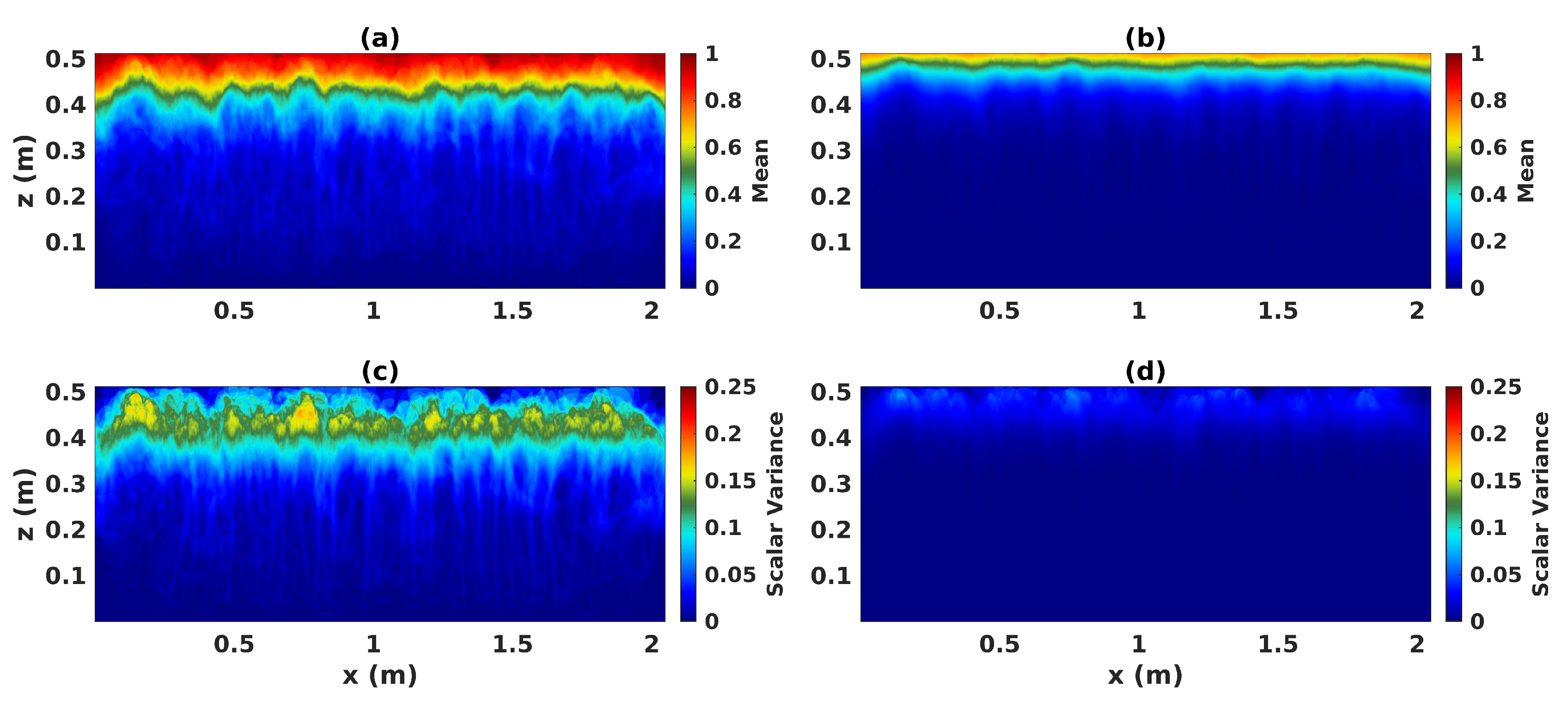
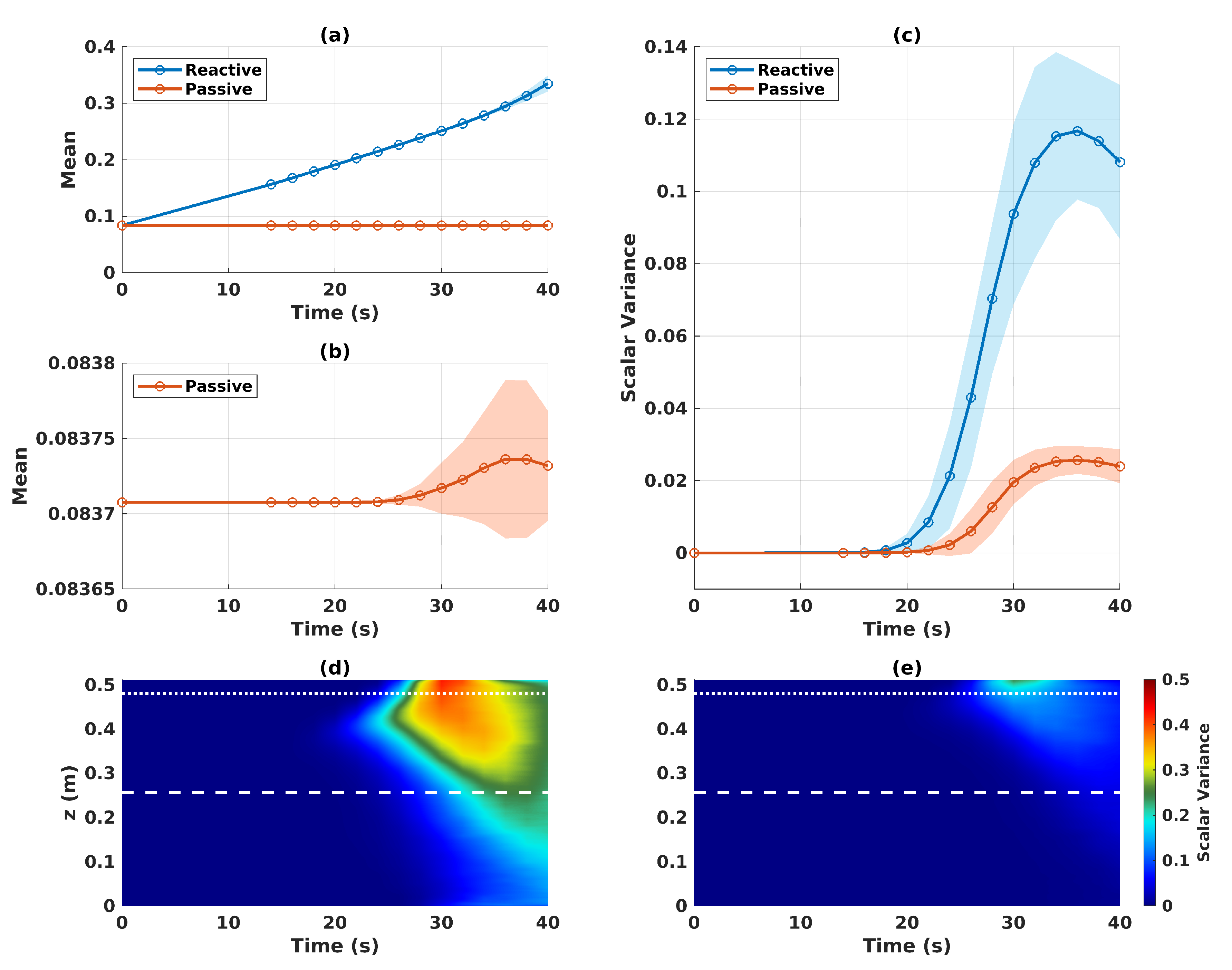
Figure 2. Mean and scalar variance of the reactive, (a) and (c), and passive, (b) and (d) tracers at $t=26$s. Panels (a) and (c) are from supplementary movie S1 and panels (b) and (d) are from S2.

Figure 2. Mean and scalar variance of the reactive, (a) and (c), and passive, (b) and (d) tracers at $t=26$s. Panels (a) and (c) are from supplementary movie S1 and panels (b) and (d) are from S2.

Figure 3. (a) Bulk mean tracer concentrations and (c) bulk scalar variances for the reactive (blue) and passive (orange) tracers. Changes in the bulk mean passive tracer concentration,(b), are $O(1e-5)$. Shaded areas extend two standard deviations away from the mean. Panels (d) and (e) depict the scalar variance integrated with respect to x for the reactive and passive tracers respectively.

Figure 3. (a) Bulk mean tracer concentrations and (c) bulk scalar variances for the reactive (blue) and passive (orange) tracers. Changes in the bulk mean passive tracer concentration,(b), are $O(1e-5)$. Shaded areas extend two standard deviations away from the mean. Panels (d) and (e) depict the scalar variance integrated with respect to x for the reactive and passive tracers respectively.

The ensemble is designed for the RT plumes in each simulation to have different spatial distributions. In each simulation, the RT bubbles (plumes of light fluid rising into heavy fluid with mushroom-shaped heads) push up against the tracer front and the tracer concentration is displaced upwards and outwards around the bubble. Meanwhile, spikes entrain the tracers into the lower parts of the domain causing the streaks observed in Figure 2. Shear causes vorticial structures to form on the undersides of the mushroom-shaped plume heads. These vortices are the first manifestation of turbulence in the flow and begin mixing the tracer that is displaced around the RT bubbles.

However, this behaviour is not obvious in the supplementary movies showing the evolution of the mean and scalar variance fields for each of the tracers. When taking the mean of an ensemble, the structures present in the flows of the individual simulations are averaged out. So, the mean tracer fields do not show any of the coherent structures that characterize turbulent mixing. Instead, the structures are captured by the fluctuations which are defined for each ensemble member as the difference between itself and the ensemble mean. The tracer fields in each of the simulations begin to differ from the mean as soon as the RT plumes start to affect their spatial distribution. Panel (c) of Figure 3 indicates a sharp increase in the scalar variance of the reactive tracer (blue) at $t=18$s as the RT bubbles reach the tracer front. It takes longer for the plumes to reach the passive tracer front.

The turbulence in each of the simulations deforms and contorts material volumes of the conserved scalar, in this case our passive tracer, and increases the magnitude of local scalar gradients. This in turn enhances molecular diffusion[51]. When this same process acts on the reactive tracer, the reaction occurring within the material volume complicates things further. For growth governed by Fisher’s equation, the concentration in each material volume increases towards the stable equilibrium value $\theta =1$ thereby increasing the rate of molecular diffusion. This doubly enhanced diffusion allows the reactive tracer to spread to areas a passive tracer may not be able to reach. Further enhancement results as the process of deformation by the flow is repeated.

Scalar variance acts as a sink in the mean ADR equation for the reactive tracer (equation13) and as a source in the fluctuation equation (equation). The fluctuations are effectively taking concentration from the mean field in addition to growing according to Fisher’s equation. In panels (a) and (c) of Figure 2 the spatial distribution of the scalar variance matches the front of the mean field. Looking at supplementary movie S1, we see that as the mean descends in the domain, its concentration is transferred to the scalar variance which evolves into a band spanning the domain horizontally. Eventually, the system becomes so well-mixed that the differences between simulations become less noticeable and thus the scalar variance decreases, Figure 3 panel (c).

Comparing the evolution of the reactive tracer with that of the passive tracer we see that in the latter case the RT instabilities quickly break the mean structure apart thereby increasing the scalar variance. However, the magnitude of the scalar variance is limited by the initial concentration of the tracer. In panels (d) and (e) of Figure 3, the reactive and passive scalar variances are integrated with respect to x and plotted as a function of depth and time. The dotted white lines indicate the inflection point of the hyperbolic tangent function describing the initial tracer distribution and the dashed line indicates the height of the mean initial density stratification. It is apparent that the reactive tracer’s scalar variance begins to increase lower in the domain as the tracer front has extended downwards. We also notice that it propagates both upwards and downwards. The upwards propagation corresponds to the transfer of concentration from the mean and to the fluctuations while the downwards propagation is uniquely due to RT induced turbulent mixing. The scalar variance of the passive tracer can only propagate downwards and is significantly smaller in magnitude.

3.2. Reynolds Stresses

The bulk absolute values of the Reynolds stresses are depicted as functions of time in panel (a) of Figure 4. The shear stress is much weaker than the other stresses (though still on the same order of magnitude) and we note $R_{22}$ varies the most between ensemble members. Panels (b) though (d) show the normalized Reynolds stresses integrated with respect to x as a function of z and time. The dashed white lines indicate the initial height of the mean density stratification. From panel (d) we see that $R_{22}$ spreads symmetrically from the location of the initial stratification which is in agreement with RT theory. The spatial distribution of $R_{11}$, panel (b), indicates that fluctuations in the horizontal velocity are symmetrical in z, greatest along the sidewalls, and take longer to increase than those in the vertical. The distribution of the shear stress is very different from those of $R_{11}$ and $R_{22}$. There is no symmetry around the initial stratification nor is there a coherent pattern.

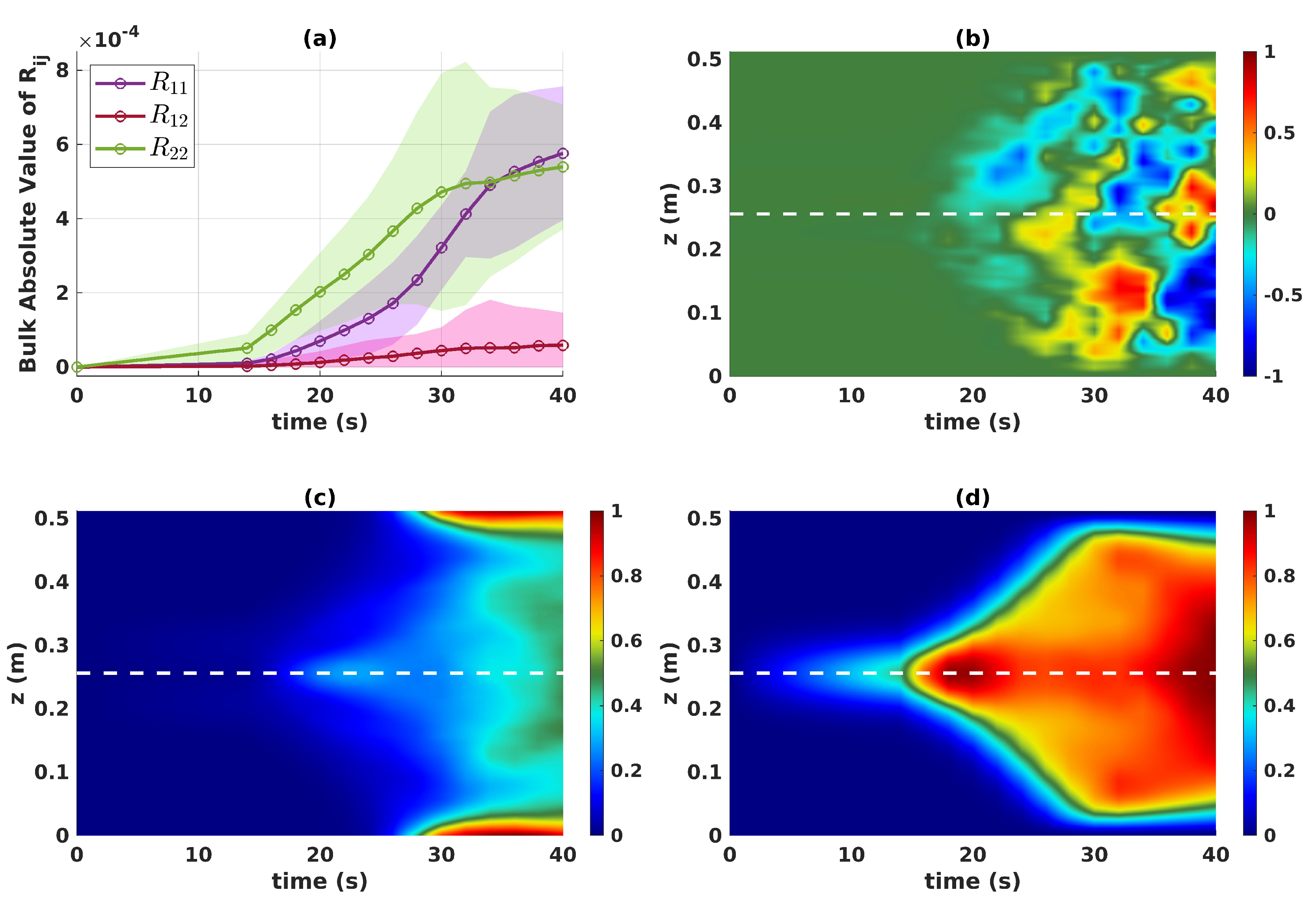
Figure 4. (a) Bulk absolute Reynolds stresses $R_{11}$ (purple), $R_{12}$ (pink), and $R_{22}$ (green) with shaded areas extending two standard deviations away from the mean (but not crossing $R_{ij}=0$). The normalized Reynolds stresses (b) $R_{12}$, (c)$R_{11}$, and (d)$R_{22}$ integrated with respect to x. Note that panel (b) has different colorbar limits as it is the only quantity that is not positive definite.

Figure 4. (a) Bulk absolute Reynolds stresses $R_{11}$ (purple), $R_{12}$ (pink), and $R_{22}$ (green) with shaded areas extending two standard deviations away from the mean (but not crossing $R_{ij}=0$). The normalized Reynolds stresses (b) $R_{12}$, (c)$R_{11}$, and (d)$R_{22}$ integrated with respect to x. Note that panel (b) has different colorbar limits as it is the only quantity that is not positive definite.

When using an eddy viscosity parameterization for the Reynolds stresses, we have[18]

$$\begin{array}{c}\hfill \overline{u^{\prime }{u}^{\prime }}={\nu }_e^{11}{U}_x,\overline{w^{\prime }{w}^{\prime }}={\nu }_e^{22}{W}_z,\overline{u^{\prime }{w}^{\prime }}={\nu }_e^{12}(U_z+W_x)/2,\end{array}$$

(19)

and values for the eddy viscosities need to be selected. Since we know the values for the Reynolds stresses and gradients of the mean velocity fields, we can divide through by the gradients to obtain time-dependent values for the eddy viscosities. In Figure 5 the Reynolds stresses and shaded areas are scaled by the maximum values of the ensemble means. The black lines indicate the corresponding normalized right hand side of the equations in 19. Panel (d) shows the time-dependent eddy viscosities resulting from the aforementioned division. The trends captured by the Reynolds stresses are not well represented by the gradients of the mean velocity fields. In particular, while the Reynolds stresses are increasing monotonically, the gradients reach their maxima around $t=30$s and then begin to decrease. The vertical eddy viscosity, ${\nu }_e^{22}$ is the largest and the most variable. This is not entirely surprising for a RT flow as the instability manifests as plumes moving primarily in the vertical. That said, if one were to run a RANS simulation using these eddy viscosity values in their eddy viscosity parameterization, they would find the mean velocity fields to be more resistant to vertical deformations than horizontal ones, which is perhaps the opposite of what one would expect of a RT flow. In fact, in Figure 4, we saw that the vertical and horizontal Reynolds stresses have similar magnitudes (because the perturbations to the initial density stratification cause plumes to propagate diagonally) but this is clearly not captured in the gradients of the mean velocity fields.

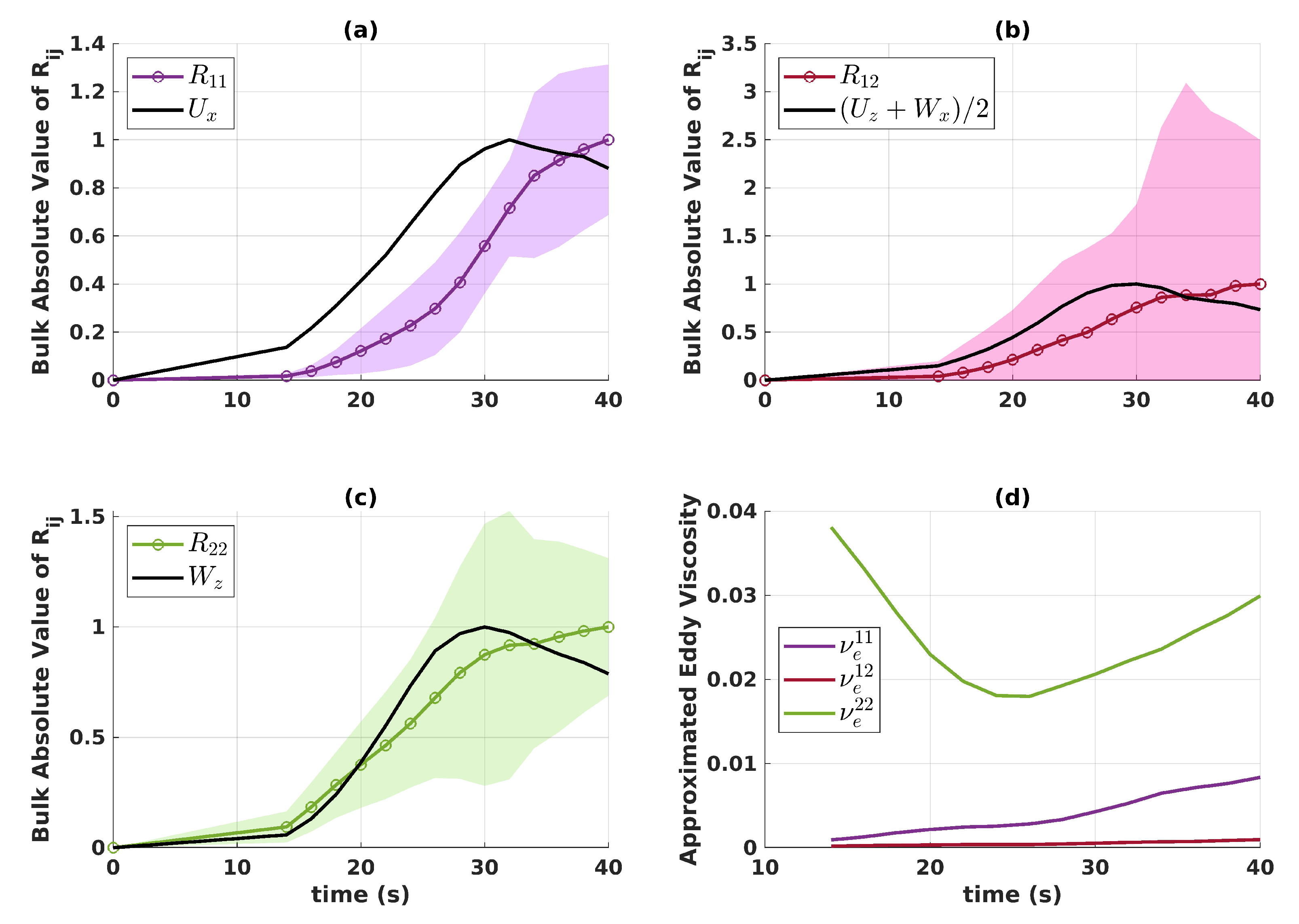
Figure 5. Normalized bulk mean Reynolds stresses (a) $R_{11}$, (b)$R_{12}$, and (c)$R_{22}$ with shaded areas extending two standard deviations away from the mean. The corresponding normalized bulk gradient approximations (a) $U_x$, (b)$(U_z+W_z)/2$, and (c) $W_z$ are plotted with black lines. The eddy viscosity values resulting from dividing the bulk Reynolds stresses by their gradient approximations are shown in (d).

Figure 5. Normalized bulk mean Reynolds stresses (a) $R_{11}$, (b)$R_{12}$, and (c)$R_{22}$ with shaded areas extending two standard deviations away from the mean. The corresponding normalized bulk gradient approximations (a) $U_x$, (b)$(U_z+W_z)/2$, and (c) $W_z$ are plotted with black lines. The eddy viscosity values resulting from dividing the bulk Reynolds stresses by their gradient approximations are shown in (d).

3.3. Eddy Fluxes

Eddy fluxes quantify the mean transport of tracer fluctuations by fluctuations in the velocity fields. In Section 3.2 the evolution of the fluctuations in the velocity fields was discussed. We saw that fluctuations in the vertical velocity component spread symmetrically from the location of the initial density stratification while fluctuations in the horizontal one are largely found along the top and bottom boundaries. In Figure 6, we compare the bulk absolute horizontal and vertical eddy fluxes in panels (a) and (b) for the reactive (blue) and passive (orange) tracers. In Section 3.1 we saw that reactive tracer fluctuations are larger than those of the passive tracer. It thus comes as no surprise that the eddy fluxes of the reactive tracer are greater than those of the passive tracer.

Despite the magnitudes of the horizontal, $R^{11}$, and vertical, $R^{22}$, Reynolds stresses being similar, it is clear that the tracer fluctuations are more closely correlated with the vertical velocity fluctuations than the horizontal ones. Around $t=30$s, the heads of the RT plumes collide with the top and bottom boundaries of the domain. At this time, the vertical eddy fluxes reach their maxima and subsequently decrease because the tracers cannot be advected any further in the vertical. The decrease in the vertical eddy flux of the reactive tracer is more dramatic than that corresponding to the passive tracer since fluctuations in the passive tracer barely reach the bottom of the domain and thus are not significantly affected by the bottom boundary.

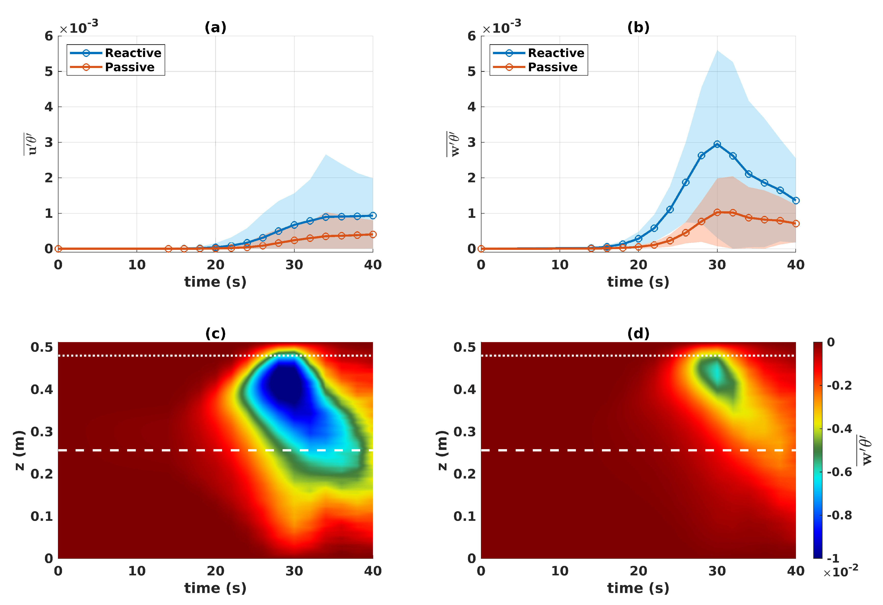
Figure 6. Bulk absolute value of the (a) horizontal, $\overline{u^{\prime }{\theta }^{\prime }}$, and (b) vertical, $\overline{w^{\prime }{\theta }^{\prime }}$, eddy fluxes of the reactive (blue) and passive (orange) tracers. Vertical eddy fluxes integrated with respect to x for the (c) reactive and (d) passive tracers.

Figure 6. Bulk absolute value of the (a) horizontal, $\overline{u^{\prime }{\theta }^{\prime }}$, and (b) vertical, $\overline{w^{\prime }{\theta }^{\prime }}$, eddy fluxes of the reactive (blue) and passive (orange) tracers. Vertical eddy fluxes integrated with respect to x for the (c) reactive and (d) passive tracers.

In panels (c) and (d) of Figure 6, the vertical eddy fluxes of the reactive and passive tracers are integrated with respect to x and shown as functions of depth and time. The dotted white lines indicate the inflection point of the hyperbolic tangent function describing the initial tracer distribution and the dashed lines indicate the initial height of the mean density stratification. For both tracers, the vertical eddy fluxes are negative because, as shown in the supplementary movies, the fluctuations are travelling downwards and the heights at which the eddy fluxes first become nonzero align with the locations of the tracer fronts. The reactive tracer fluctuations and fluctuations in the vertical velocity field both propagate upwards (Figure 3 and Figure 4) making the vertical eddy flux propagate upwards. This does not necessarily imply that the fluctuations are being transported upwards. Rather, it tells us that the fluctuations develop higher in the domain as they consume concentration from the front of the mean distribution. This is particularly evident in supplementary movie of the reactive tracer fields (S1). These space-time plots further support the conclusion that the decrease seen in the bulk absolute vertical eddy flux of the reactive tracer is more dramatic because fluctuations in the passive tracer barely extend to the bottom of the domain.

When running RANS simulations, eddy diffusivity parameterizations of the form

$$\begin{array}{c}\hfill \overline{u^{\prime }{\theta }^{\prime }}={\kappa }_H\frac{\partial \theta }{\partial x},\overline{w^{\prime }{\theta }^{\prime }}={\kappa }_V\frac{\partial \theta }{\partial z},\end{array}$$

(20)

are often used in place of the eddy fluxes which are unknown. In Section 3.2, we saw that the eddy viscosity parameterization does not capture the same trends as the Reynolds stresses if the eddy viscosities are assumed to be constant. This does not inspire much confidence in the performance of the analogous eddy diffusivity parameterization. In panels (a) and (b) of Figure 7 the normalized bulk absolute eddy fluxes are plotted along with the normalized right hand sides of the equations in 20. The tracer derivatives taken with respect to x capture the general behaviour of the horizontal eddy fluxes but fail to capture the details. The horizontal eddy fluxes start increasing earlier and begin to plateau at late times. The tracer derivatives taken with respect to z increase monotonically and clearly do not capture the behaviour of the vertical eddy fluxes which peak around $t=30$s and then begin to decrease. As previously discussed, the vertical eddy fluxes peak when tracer fluctuations reach the bottom of the domain. Eddy diffusivity parameterizations consider the gradient of the tracer mean which only begins to reach the bottom boundary when the simulations are stopped and the tracer is well-mixed. In panels (c) and (d), we plot the corresponding vertical and horizontal eddy diffusivities obtained from dividing through by the tracer derivatives. We immediately note that the horizontal eddy diffusivities are two orders of magnitude smaller than the vertical ones. The variability in the values brings the use of constant eddy diffusivities into question.

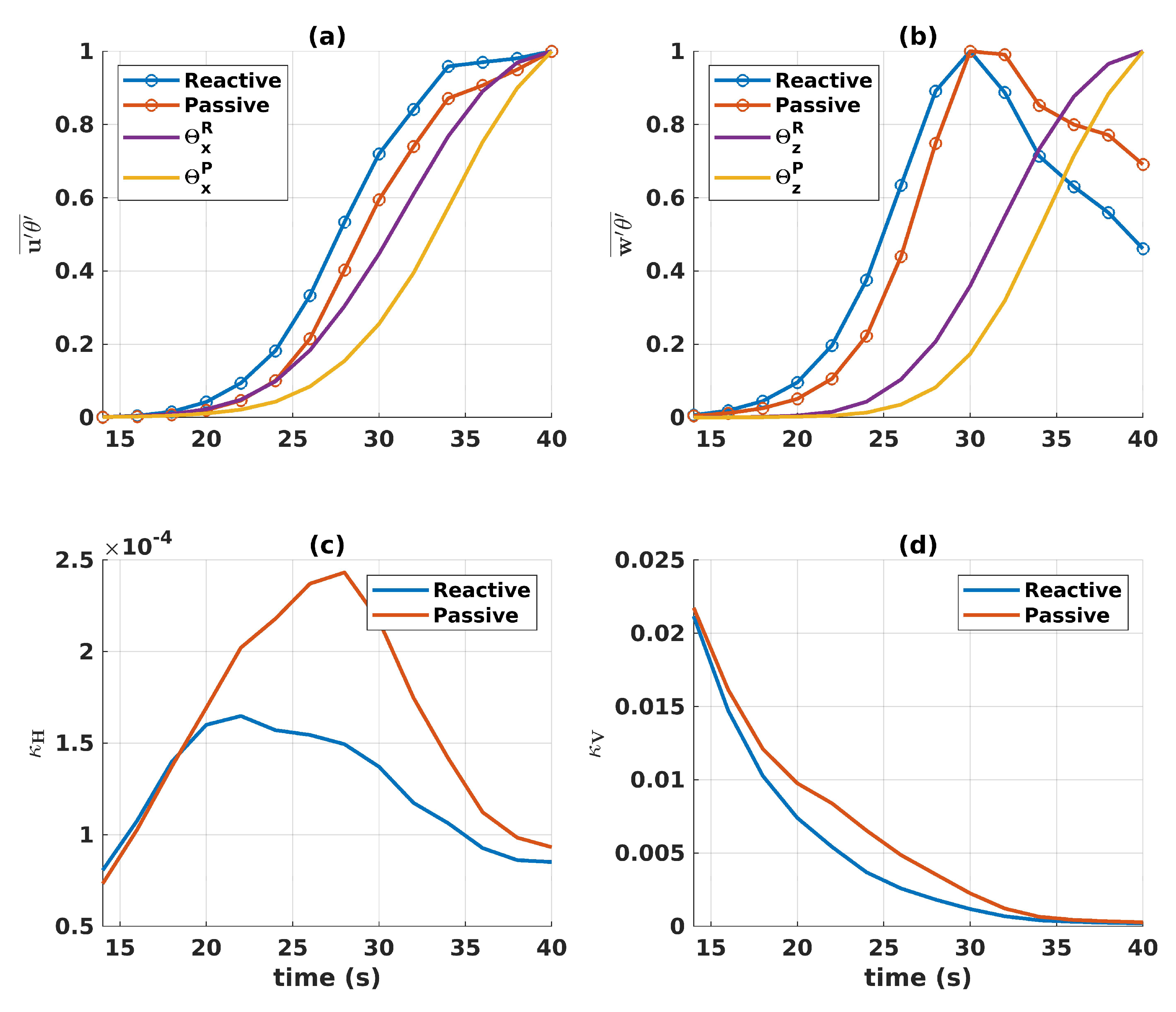
Figure 7. Normalized bulk absolute values of the (a) horizontal, $\overline{u^{\prime }{\theta }^{\prime }}$, and (b) vertical, $\overline{w^{\prime }{\theta }^{\prime }}$, eddy fluxes of the reactive (blue) and passive (orange) tracers. The bulk absolute values of the derivatives of the tracers with respect to (a) x and (b) z are shown in purple and yellow for the reactive and passive tracers respectively. The (c) horizontal, $k_H=\overline{u^{\prime }{\theta }^{\prime }}/{\theta }_x$, and (d) vertical, $k_V=\overline{w^{\prime }{\theta }^{\prime }}/{\theta }_z$, eddy diffusivities are plotted as functions of time.

Figure 7. Normalized bulk absolute values of the (a) horizontal, $\overline{u^{\prime }{\theta }^{\prime }}$, and (b) vertical, $\overline{w^{\prime }{\theta }^{\prime }}$, eddy fluxes of the reactive (blue) and passive (orange) tracers. The bulk absolute values of the derivatives of the tracers with respect to (a) x and (b) z are shown in purple and yellow for the reactive and passive tracers respectively. The (c) horizontal, $k_H=\overline{u^{\prime }{\theta }^{\prime }}/{\theta }_x$, and (d) vertical, $k_V=\overline{w^{\prime }{\theta }^{\prime }}/{\theta }_z$, eddy diffusivities are plotted as functions of time.

Bulk descriptions do not capture any information about the directions of the eddy fluxes or gradients. The angle between the vectors $({\Theta }_x,{\Theta }_z)$ and $(\overline{u^{\prime }{\theta }^{\prime }},\overline{w^{\prime }{\theta }^{\prime }})$ can be calculated at each grid point and indicates whether the eddy diffusivity parameterization is diffusing the tracer in the right direction. The data bins nicely into two groups, one centred around 0, and another centred around $\pm \pi$. As shown in panels (b) and (c) of Figure 8, the spread within the bins, indicated by the shaded area extending two standard deviations away from the mean of the bin, is $O\left(0.1\right)$. In panel (a), the percentage of grid points in either bin is plotted as a function of time for both the reactive and passive tracers. The percentage of points in each bin always lies within $\pm 2\%$ of 50% and, for most times, there are more points in the bin centred at 0.

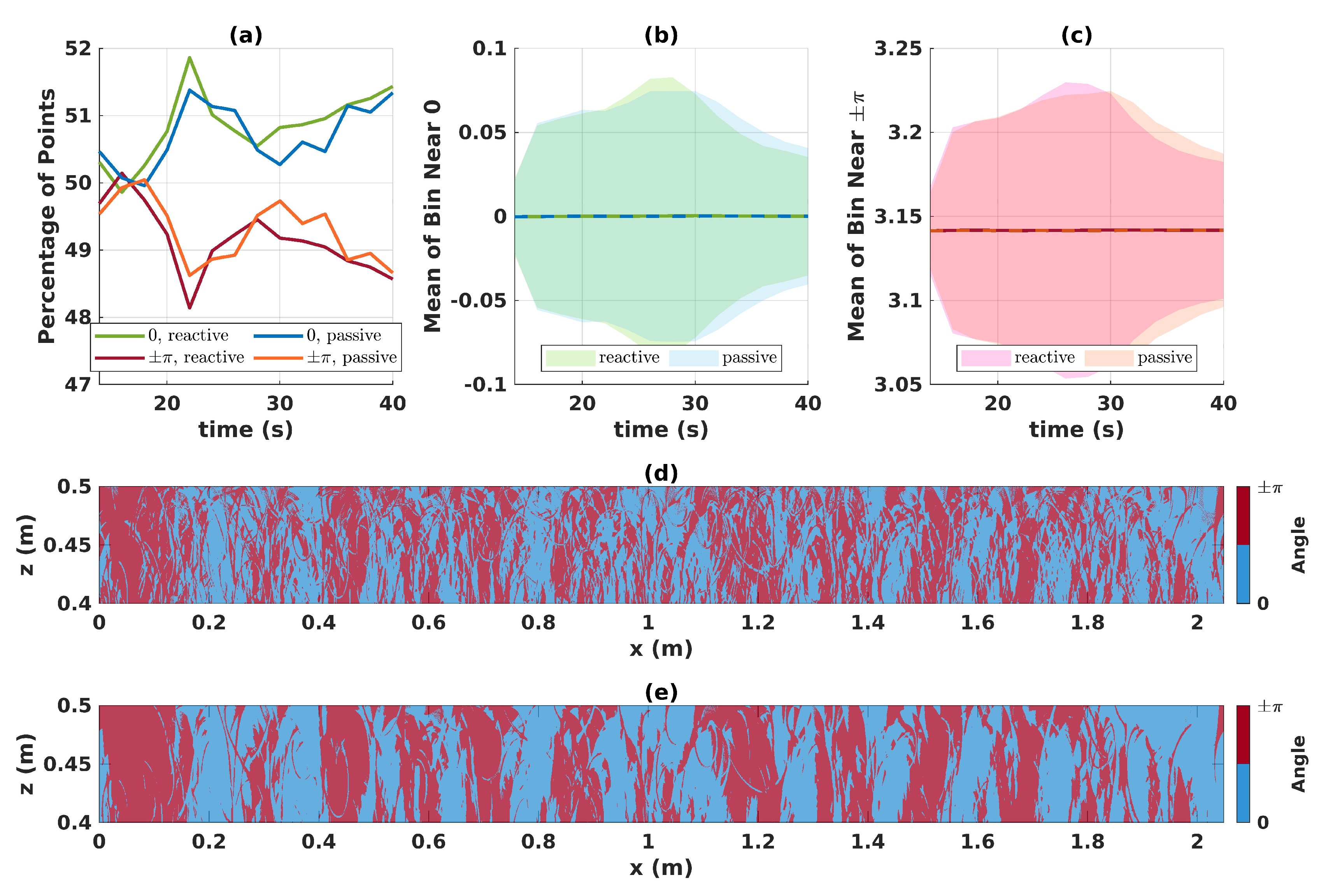
Figure 8. The angle between the eddy flux and gradient vectors is calculated at each grid point. The data bins nicely into two groups centred around 0 and $\pm \pi$. In (a), the percentage of points in each bin is shown for the reactive (green, red) and passive (blue, orange) tracers. The means of the (b) 0 and (c) $\pm \pi$ bins are indicated by lines and the shaded areas extend two standard deviations away from the mean indicating the spread within each bin is reasonable. The spatial distribution of the binned points at $t=26$s and within a subdomain is shown for the (d) reactive and (c) passive tracers.

Figure 8. The angle between the eddy flux and gradient vectors is calculated at each grid point. The data bins nicely into two groups centred around 0 and $\pm \pi$. In (a), the percentage of points in each bin is shown for the reactive (green, red) and passive (blue, orange) tracers. The means of the (b) 0 and (c) $\pm \pi$ bins are indicated by lines and the shaded areas extend two standard deviations away from the mean indicating the spread within each bin is reasonable. The spatial distribution of the binned points at $t=26$s and within a subdomain is shown for the (d) reactive and (c) passive tracers.

The eddy fluxes and gradients are either almost perfectly parallel or nearly pointing in opposite directions. In the later case, a negative eddy diffusivity is needed to realign the vectors. The spatial distribution of the binned grid points at $t=26$s within a subdomain is shown for the reactive and passive tracers in panels (d) and (e) of Figure 8. In the red areas, the eddy fluxes and gradients are binned as anti-parallel and a negative eddy diffusivity is implied. The binned grid points self organize into columns, though the columns are less well-defined for the reactive tracer. The issue of negative diffusivities will be revisited in the discussion.

The plumes formed by RT instabilities primarily move vertically, though the perturbations applied to the initial density stratification do encourage some plumes to propagate diagonally. If we consider the mean initial stratification, the perturbations average out. So, the mean effect of the RT instabilities is to transport the tracers vertically until turbulent mixing becomes strong enough to induce horizontal transport. The stills in panels (d) and (e) of Figure 8 are taken just before the heads of the RT plumes reach the top of the domain after which point turbulent mixing dominates. Since eddy fluxes are an averaged quantity, they too are arranged into columns.

Meanwhile, the mean tracer concentration lies largely in a band along the top of the domain as shown in panels (a) and (b) of Figure 2. The gradient of the mean thus generally points downwards. So, while the eddy fluxes reflect properties of the flow governing the tracer transport, the gradients only reflect the spatial distribution of the mean tracer field.

The distribution of the binned data corresponding to the reactive tracer, panel (d) Figure 8, is more disorganized because the RT bubbles have already reached the mean tracer front. As previously mentioned, the increased Fickian diffusion exhibited by the reactive tracer will allow it to diffuse and then be further entrained into regions the passive tracer may not be able to reach. The reaction, then causes this process to be repeated, enriching the fluctuation field.

4. Discussion

Abbreviations

References

1. Triantafyllou, G.; Yao, F.; Petihakis, G.; Tsiaras, K.; Raitsos, D.; Hoteit, I. Exploring the Red Sea seasonal ecosystem functioning using a three-dimensional biophysical model. Journal of Geophysical Research: Oceans 2014, 119, 1791–1811. [Google Scholar] [CrossRef]
2. KAMYKowski, D. A preliminary biophysical model of the relationship between temperature and plant nutrients in the upper ocean. Deep Sea Research Part A. Oceanographic Research Papers 1987, 34, 1067–1079. [Google Scholar] [CrossRef]
3. Resplandy, L.; Lévy, M.; McGillicuddy Jr, D.J. Effects of eddy-driven subduction on ocean biological carbon pump. Global Biogeochemical Cycles 2019, 33, 1071–1084. [Google Scholar] [CrossRef]
4. Goldstein, E.D.; Pirtle, J.L.; Duffy-Anderson, J.T.; Stockhausen, W.T.; Zimmermann, M.; Wilson, M.T.; Mordy, C.W. Eddy retention and seafloor terrain facilitate cross-shelf transport and delivery of fish larvae to suitable nursery habitats. Limnology and Oceanography 2020, 65, 2800–2818. [Google Scholar] [CrossRef]
5. Baustian, M.M.; Meselhe, E.; Jung, H.; Sadid, K.; Duke-Sylvester, S.M.; Visser, J.M.; Allison, M.A.; Moss, L.C.; Ramatchandirane, C.; van Maren, D.S.; others. Development of an Integrated Biophysical Model to represent morphological and ecological processes in a changing deltaic and coastal ecosystem. Environmental Modelling & Software 2018, 109, 402–419. [Google Scholar] [CrossRef]
6. Laurent, A.; Fennel, K.; Kuhn, A. An observation-based evaluation and ranking of historical Earth system model simulations in the northwest North Atlantic Ocean. Biogeosciences 2021, 18, 1803–1822. [Google Scholar] [CrossRef]
7. Haidvogel, D.B.; Arango, H.; Budgell, W.P.; Cornuelle, B.D.; Curchitser, E.; Di Lorenzo, E.; Fennel, K.; Geyer, W.R.; Hermann, A.J.; Lanerolle, L.; others. Ocean forecasting in terrain-following coordinates: Formulation and skill assessment of the Regional Ocean Modeling System. Journal of computational physics 2008, 227, 3595–3624. [Google Scholar] [CrossRef]
8. Higdon, R.L.; Bennett, A.F. Stability analysis of operator splitting for large-scale ocean modeling. Journal of Computational Physics 1996, 123, 311–329. [Google Scholar] [CrossRef]
9. Shchepetkin, A.F.; McWilliams, J.C. The regional oceanic modeling system (ROMS): a split-explicit, free-surface, topography-following-coordinate oceanic model. Ocean modelling 2005, 9, 347–404. [Google Scholar] [CrossRef]
10. ROMS Wiki Vertical Mixing Parameterizations. https://www.myroms.org/wiki/Vertical_Mixing_Parameterizations. Accessed: 2023-08-18.
11. Burchard, H.; Rennau, H. Comparative quantification of physically and numerically induced mixing in ocean models. Ocean Modelling 2008, 20, 293–311. [Google Scholar] [CrossRef]
12. Brennan, C.E.; Bianucci, L.; Fennel, K. Sensitivity of northwest North Atlantic shelf circulation to surface and boundary forcing: A regional model assessment. Atmosphere-Ocean 2016, 54, 230–247. [Google Scholar] [CrossRef]
13. Kumar, R.; Li, J.; Hedstrom, K.; Babanin, A.V.; Holland, D.M.; Heil, P.; Tang, Y. Intercomparison of Arctic sea ice simulation in ROMS-CICE and ROMS-Budgell. Polar Science 2021, 29, 100716. [Google Scholar] [CrossRef]
14. Sui, Y.; Sheng, J.; Tang, D.; Xing, J. Study of storm-induced changes in circulation and temperature over the northern South China Sea during Typhoon Linfa. Continental Shelf Research 2022, 249, 104866. [Google Scholar] [CrossRef]
15. Pope, S.B. Turbulent flows; Cambridge university press, 2000.
16. Dimotakis, P.E. Turbulent mixing. Annu. Rev. Fluid Mech. 2005, 37, 329–356. [Google Scholar] [CrossRef]
17. Sreenivasan, K.R. Turbulent mixing: A perspective. Proceedings of the National Academy of Sciences 2019, 116, 18175–18183. [Google Scholar] [CrossRef]
18. Kundu, P.K.; Cohen, I.M.; Dowling, D.R. Fluid mechanics; Academic press, 2015.
19. Alfonsi, G. Reynolds-averaged Navier–Stokes equations for turbulence modeling 2009.
20. Xiao, H.; Cinnella, P. Quantification of model uncertainty in RANS simulations: A review. Progress in Aerospace Sciences 2019, 108, 1–31. [Google Scholar] [CrossRef]
21. Pozorski, J.; Minier, J.P. Modeling scalar mixing process in turbulent flow. First Symposium on Turbulence and Shear Flow Phenomena. Begel House Inc., 1999.
22. Abernathey, R.P.; Marshall, J. Global surface eddy diffusivities derived from satellite altimetry. Journal of Geophysical Research: Oceans 2013, 118, 901–916. [Google Scholar] [CrossRef]
23. Cole, S.T.; Wortham, C.; Kunze, E.; Owens, W.B. Eddy stirring and horizontal diffusivity from Argo float observations: Geographic and depth variability. Geophysical Research Letters 2015, 42, 3989–3997. [Google Scholar] [CrossRef]
24. Marshall, J.; Shuckburgh, E.; Jones, H.; Hill, C. Estimates and implications of surface eddy diffusivity in the Southern Ocean derived from tracer transport. Journal of physical oceanography 2006, 36, 1806–1821. [Google Scholar] [CrossRef]
25. Sallée, J.; Speer, K.; Morrow, R.; Lumpkin, R. An estimate of Lagrangian eddy statistics and diffusion in the mixed layer of the Southern Ocean. Journal of Marine Research 2008, 66, 441–463.
26. Ferrari, R.; Nikurashin, M. Suppression of eddy diffusivity across jets in the Southern Ocean. Journal of Physical Oceanography 2010, 40, 1501–1519. [Google Scholar] [CrossRef]
27. Holloway, G. Estimation of oceanic eddy transports from satellite altimetry. Nature 1986, 323, 243–244. [Google Scholar] [CrossRef]
28. Gargett, A.E. Vertical eddy diffusivity in the ocean interior. Journal of Marine Research 1984, 42, 359–393. [Google Scholar] [CrossRef]
29. Kamenkovich, I.; Berloff, P.; Haigh, M.; Sun, L.; Lu, Y. Complexity of mesoscale eddy diffusivity in the ocean. Geophysical Research Letters 2021, 48, e2020GL091719. [Google Scholar] [CrossRef]
30. Smith, K.M.; Hamlington, P.E.; Fox-Kemper, B. Effects of submesoscale turbulence on ocean tracers. Journal of Geophysical Research: Oceans 2016, 121, 908–933. [Google Scholar] [CrossRef]
31. Radko, T. Double-diffusive convection; Cambridge University Press, 2013.
32. Bachman, S.D.; Fox-Kemper, B.; Bryan, F.O. A tracer-based inversion method for diagnosing eddy-induced diffusivity and advection. Ocean Modelling 2015, 86, 1–14. [Google Scholar] [CrossRef]
33. Pasquero, C. Differential eddy diffusion of biogeochemical tracers. Geophysical research letters 2005, 32. [Google Scholar] [CrossRef]
34. Tergolina, V.B.; Calzavarini, E.; Mompean, G.; Berti, S. Effects of large-scale advection and small-scale turbulent diffusion on vertical phytoplankton dynamics. Physical Review E 2021, 104, 065106. [Google Scholar] [CrossRef] [PubMed]
35. Richards, K.J.; Brentnall, S.J. The impact of diffusion and stirring on the dynamics of interacting populations. Journal of theoretical biology 2006, 238, 340–347. [Google Scholar] [CrossRef] [PubMed]
36. Lévy, M.; Martin, A.P. The influence of mesoscale and submesoscale heterogeneity on ocean biogeochemical reactions. Global Biogeochemical Cycles 2013, 27, 1139–1150. [Google Scholar] [CrossRef]
37. Zhang, J.; Tejada-Martínez, A.E.; Zhang, Q. Developments in computational fluid dynamics-based modeling for disinfection technologies over the last two decades: A review. Environmental modelling & software 2014, 58, 71–85. [Google Scholar] [CrossRef]
38. Zhang, J.; Tejada-Martínez, A.E.; Zhang, Q.; Lei, H. Evaluating hydraulic and disinfection efficiencies of a full-scale ozone contactor using a RANS-based modeling framework. Water Research 2014, 52, 155–167. [Google Scholar] [CrossRef]
39. Angeloudis, A.; Stoesser, T.; Gualtieri, C.; Falconer, R.; others. Effect of three-dimensional mixing conditions on water treatment reaction processes. Proceedings of the 36th IAHR World Congress. The Netherlands: The Hague, 2015.
40. Weerasuriya, A.U.; Zhang, X.; Tse, K.T.; Liu, C.H.; Kwok, K.C. RANS simulation of near-field dispersion of reactive air pollutants. Building and Environment 2022, 207, 108553. [Google Scholar] [CrossRef]
41. Aubagnac-Karkar, D.; Michel, J.B.; Colin, O.; Vervisch-Kljakic, P.E.; Darabiha, N. Sectional soot model coupled to tabulated chemistry for Diesel RANS simulations. Combustion and Flame 2015, 162, 3081–3099. [Google Scholar] [CrossRef]
42. Beltram Tergolina, V.; Calzavarini, E.; Mompean, G.; Berti, S. Surface light modulation by sea ice and phytoplankton survival in a convective flow model. arXiv e-prints 2022, pp. arXiv–2211.
43. Kelley, D.E. Convection in ice-covered lakes: effects on algal suspension. Journal of Plankton Research 1997, 19, 1859–1880.
44. Cabot, W. Comparison of two-and three-dimensional simulations of miscible Rayleigh-Taylor instability. Physics of Fluids 2006, 18. [Google Scholar] [CrossRef]
45. Kokkinakis, I.W.; Drikakis, D.; Youngs, D.L. Modeling of Rayleigh-Taylor mixing using single-fluid models. Physical Review E 2019, 99, 013104. [Google Scholar] [CrossRef]
46. Abarzhi, S.I. Review of theoretical modelling approaches of Rayleigh–Taylor instabilities and turbulent mixing. Philosophical Transactions of the Royal Society A: Mathematical, Physical and Engineering Sciences 2010, 368, 1809–1828. [Google Scholar] [CrossRef]
47. Dalziel, S.; Linden, P.; Youngs, D. Self-similarity and internal structure of turbulence induced by Rayleigh–Taylor instability. Journal of fluid Mechanics 1999, 399, 1–48. [Google Scholar] [CrossRef]
48. Zhou, Q. Temporal evolution and scaling of mixing in two-dimensional Rayleigh-Taylor turbulence. Physics of Fluids 2013, 25. [Google Scholar] [CrossRef]
49. Subich, C.J.; Lamb, K.G.; Stastna, M. Simulation of the Navier–Stokes equations in three dimensions with a spectral collocation method. International Journal for Numerical Methods in Fluids 2013, 73, 103–129. [Google Scholar] [CrossRef]
50. Bracco, A.; Clayton, S.; Pasquero, C. Horizontal advection, diffusion, and plankton spectra at the sea surface. Journal of Geophysical Research: Oceans 2009, 114. [Google Scholar] [CrossRef]
51. Wyngaard, J.C. Turbulence in the Atmosphere; Cambridge University Press, 2010.
52. Trefethen, L.N. Spectral methods in MATLAB, volume 10 of Software, Environments, and Tools. Society for Industrial and Applied Mathematics (SIAM), Philadelphia, PA 2000, 24, 57. [Google Scholar]
53. Harnanan, S.; Soontiens, N.; Stastna, M. Internal wave boundary layer interaction: A novel instability over broad topography. Physics of Fluids 2015, 27. [Google Scholar] [CrossRef]
54. Deepwell, D.; Stastna, M.; Carr, M.; Davies, P.A. Interaction of a mode-2 internal solitary wave with narrow isolated topography. Physics of Fluids 2017, 29. [Google Scholar] [CrossRef]
55. Prend, C.J.; Flierl, G.R.; Smith, K.M.; Kaminski, A.K. Parameterizing eddy transport of biogeochemical tracers. Geophysical Research Letters 2021, 48, e2021GL094405. [Google Scholar] [CrossRef]
56. Hopkins, J.E.; Palmer, M.R.; Poulton, A.J.; Hickman, A.E.; Sharples, J. Control of a phytoplankton bloom by wind-driven vertical mixing and light availability. Limnology and Oceanography 2021, 66, 1926–1949. [Google Scholar] [CrossRef]
57. Rutherford, K.; Fennel, K.; Atamanchuk, D.; Wallace, D.; Thomas, H. A modelling study of temporal and spatial pCO 2 variability on the biologically active and temperature-dominated Scotian Shelf. Biogeosciences 2021, 18, 6271–6286. [Google Scholar] [CrossRef]