
Submitted:
12 September 2023
Posted:
14 September 2023
You are already at the latest version
Abstract
In this paper, we continue the research cycle on the properties of convolutional neural network-based image recognition systems and ways to improve noise immunity and robustness [1]. Currently, a popular research area related to artificial neural networks is adversarial attacks. The effect of adversarial attacks on the image is not highly perceptible to the human eye, also it drastically reduces the neural network accuracy. Image perception by a machine is highly dependent on the propagation of high frequency distortions throughout the network. At the same time, a human efficiently ignores high-frequency distortions, perceiving the shape of objects as a whole. The approach proposed in this paper can improve the image recognition accuracy in the presence of high-frequency distortions, in particular, caused by adversarial attacks. The proposed technique makes it possible to measure up the logic of artificial neural network to that of a human, for whom high-frequency distortions are not decisive in object recognition.
Keywords:
adversarial attacks
; artificial neural networks
; robustness
; image filtering
; convolutional neural networks
; image recognition
; image distortion
1. Introduction
Сonvolutional neural networks have gained a wide range of applications in modern computing since they allow to automate the wide class of tasks, such as image classification and segmentation [2], object detection and tracking in video streams [3], and image generation [4], [5]. Also, convolutional neural networks are the most effective machine learning tool for some audio processing tasks [6] [7]. Recently, an increasing part of computational processing power is involved in multimedia processing. The growth of overall computing power allows to use increasingly complex and demanding machine learning algorithms. The convolutional neural networks also allow to extract features from multimedia efficiently and process big data, so they are used to solve the difficult or fuzzy tasks.
However, a significant unsolved problem for convolutional neural networks is their sensitivity to distortions and noise. Neural networks trained using clean data do not provide sufficient generalizability to recognize distorted or noisy images. So far, the precise noise/distortion robustness characteristics of convolutional neural networks are unknown yet, only few studies in this field are available up to date [8] [9] [10]. The adversarial distortions severely reduce the image recognition accuracy since they are targeted to the exact neural network model. One of the first mentions of this problem is the study [11], which demonstrated, among other limitations, the weaknesses in the neural network’s generalization ability. The authors have also found out that adversarial distortions are relatively effective for variety of neural networks with a diverse number of layers, architectures, or trained using different datasets. Adversarial images are transferable to other neural networks, even if these networks are trained with different hyperparameters or dataset. Later, a range of techniques for generating adversarial examples were proposed, including FGSM [12], Deepfool [13], One-pixel attack [14] [15], and many others. The maxout network [16], initially achieving an error probability of 0.45%, after application of Fast Gradient Sign Method (FGSM) misclassified 89.4% of adversarial examples, with an average confidence rate of 97.6%. Moreover, with higher image resolution, the recognition error of adversarial examples increases. Currently, the “arms race” of adversarial attacks and countermeasures is relevant [17] [18] [19].
Numerous digitally presented natural images also have distortions induced during the imaging process. Such distortions appear in the images without the attacker’s involvement (unusual camera angles and perspectives, camera matrix thermal noise and lens specifics, atmospheric distortions, image digitization and compression artefacts). Natural adversarial examples are unpredictable, so the corresponding mitigation methods are often not obvious.
These distortions are referred as domain shifts [20] and can be exploited by attackers [21]. One of the first works on natural adversarial examples is [22]. Basing on the ImageNet dataset, which includes tens of millions of images, the authors created datasets (ImageNet-A and ImageNet-O) containing images that are the worst recognized by the state-of-the-art machine learning models. At the same time, the images presented by the authors contain a limited number of false features (Figure 1).
State-of-the-art convolutional network models such as AlexNet, DenseNet-121, ResNet-50, SqueezeNet, and VGG-19 achieve a recognition accuracy no higher than 2.2% on the ImageNet-A dataset (which is approximately 90% lower than the recognition accuracy of the ImageNet dataset by the same networks). The work [22] shows that existing data augmentation methods do not improve performance significantly. Training on other public datasets provides limited improvement. However, [22] doesn’t propose efficient ways to overcome the effect of adversarial distortion.
The above-mentioned problems must be addressed in developing modern convolutional neural network-based image recognition systems.
Some works focused on mitigation methods to cope with distortions and noise in images, are known up to date [23] [24] [25] [26] [27] [28]. Some of these works propose various denoising filters, i.e., image preprocessing, generative adversarial networks and training with noisy data. Most image preprocessing systems are specific to certain types of distortions and adversarial attack designs, so they are being quickly overcome by new adversarial algorithms [29] [30]. Important requirements for denoisers, such as boundaries and textures preservation, do not give an advantage in resisting adversarial attacks.
Another known technique to provide adversarial robustness is to use two or more opposing networks. Here, a competing adversarial network generates distorted images to provide misclassification by the classifier. The classifier is trained to resist these attacks [31], [32]. Accordingly, adversarial examples can be a good source of augmentation. This augmentation method is effective for increasing the convolutional neural network robustness to unobvious and unobservable distortions. However, this approach significantly complicates the development process, the neural network training, and also requires training process monitoring, and is still not always reliable [33]. A crucial way to counteract noise and distortion in test data is to train a neural network using augmented data [34], [35]. Various methods, specific to the task, are used for data augmentation. However, a significant amount of research related to convolutional neural networks application still does not address this problem.
In this paper, we propose a technique which reduces the high-frequency noise influence on the CNNs. We adopt radio engineering principles - filtering noisy images using a low-pass Gaussian filter [36] [37]. Image filtering allows to suppress high-frequency noise, at the same time it blurs the image, reducing its sharpness. This leads to a recognition accuracy decrease, as CNN is initially trained to recognize sharp images. Thus, filtering images with a Gaussian filter allows us to reduce the problem of overcoming high-frequency adversarial attacks to the problem of blurred image recognition, considered in our previous work [38]. The essence of the proposed technique is shown in Figure 2.
To improve the recognition accuracy, it is essential to train the recognition system to recognize blurred images efficiently. It can be done by training the recognition system using augmentation with blurred images [1]. In this paper, we prove that this technique for image pre-processing effectively improves noisy image recognition accuracy without significant reduction of clean image recognition accuracy. We show the existence of an optimum for the Gaussian filter size and propose a technique for finding this optimum. We analyze and compare the behavior of two neural networks: a simple convolutional neural network and the state-of-the-art EfficientNetB3 network [39]. Our simple CNN is tested on datasets with a small number of classes on ImageNet. The EfficientNetB3 is tested on CIFAR-10, Natural Images and Rock-Paper-Scissors datasets.
2. Materials and Methods
2.1. Datasets
We used 4 datasets to train the networks and analyze the results, including CIFAR-10, ImageNet, Rock-Paper-Scissors and the Natural Images dataset.
CIFAR-10 is one of the most widely used image sets for CNN training and testing. The dataset includes 60000 images in 10 classes, the image resolution is 32×32×3 [40]. This resolution is relatively low, which, on the one hand, allows to spend much less time and computational resources for training. On the contrary, it significantly reduces the recognition accuracy of distorted or noisy images, even with low noise intensity (Figure 3).
Natural Images is a comparatively small dataset of natural images [41] consisting of 6899 images of 8 different classes (aircraft, car, cat, dog, flower, fruit, motorcycle, human) (Figure 4). Since training neural networks using large datasets such as ImageNet-1k is challenging, we used the Natural Images set to run a broad class of tests in order to reduce the time and computational cost.
ImageNet-1k [42], a subset of the ImageNet dataset, is a large dataset containing ~1.4 million images labelled into 1000 classes. The image resolution is not standardized. Images are represented in 3 channels. ImageNet-1k is widely used for testing automated image localization and classification systems, as it is rather complex in terms of feature sets and class diversity. We used the ImageNet-1k dataset to extend and validate the results of this research on a complex dataset.
The Rock-Paper-Scissors (RPS) Images dataset [43] contains images of hand gestures from the Rock-Paper-Scissors game. Images are obtained as part of a project [42] to implement a Rock-Paper-Scissors game using computer vision and machine learning. The dataset contains 2188 images corresponding to the gestures “Stone” (726 images), “Paper” (710 images) and “Scissors” (752 images). All images are made on a green background with relatively equal illumination and white balance. All images are RGB with 300×200 pixels resolution.
3.2. Convolutional Nets
In this study, we used two architectures of convolutional neural networks:
- Simplified high-speed CNN called SimConvNet; defined below;
- The commonly used EfficientNetB3 [39].
We obtained the results of the first experiments using a simplified high-performance network. The network contains 914,960 parameters, which allows us to conduct short tests at the expense of overall classification accuracy (Figure 5).
To extend the research and validate results, we used EfficientNet [39]. The research [39] highlighted that insufficient attention is paid to balancing resolution, width and depth in the new CNN architectures, and pointed out the importance of such balancing. An efficient method for the combined CNN scaling to any size is proposed in [39]. With orders of magnitude fewer parameters and training time compared to many state-of-the-art network architectures, the EfficientNetB3 architecture achieves higher Top-1 classification accuracy results on various datasets. Since we provide a broad test set in this research, we use EfficientNetB3 to limit the time and computational resources spent on experiment. It allows us to analyze complex image sets with an acceptable accuracy.
2.3. Adversarial Attacks
FGSM (Fast Gradient Sign Method) is currently one of the most popular adversarial attack methods [12]. The core idea of the method is to add some non-random vector to the original image. The direction of this vector matches the loss function gradient. FGSM additive vector can be represented as:
where θ—the neural network model parameters, x is the input vector (image), y is the true class of vector x (if available), J(θ, x, y) is the loss function, ε is the empirically chosen gain factor, ∇x is the gradient in image space.
η=ε·sgn(∇xJ(θ,x,y)),
This adversarial vector looks, to human perception, as a high-frequency, low-intensity noise that does not affect object recognition ability. However, this noise is extremely efficient in reducing object recognition accuracy by neural networks. The intensity of the attack is chosen in order to minimize the visible changes in the image and at the same time to achieve sufficient attack success rate. It is possible to perform the attack on some state-of-the-art CNN models preserving non-visibility of changes to a human (Figure 6).
Although FGSM is one of the first adversarial attack algorithms, it is considered one of the most efficient, simple to implement and fast. A more complex variant of FGSM is the PGD (projected gradient descent) algorithm. The essence of the PGD algorithm is to iterate the FGSM algorithm to improve the attack efficiency [44].
Many other adversarial attack algorithms are also based on FGSM [45]. We can presume that proposed high-frequency noise countermeasure technique can be rather efficient against high-frequency distortions such as PGD [44], C&W attack [48], ZOO [49], HSJA [50], DeepFool [13]. At the same time, we should note that the proposed technique will not work well against different adversarial attacks such as physical space attacks [46] and Square attack [47].
2.4. The theoretical approach to the problem solution
An important feature of image recognition CNNs is the low receptivity to the object’s size. It makes the influence of both low-frequency and high-frequency image components nearly equal. It is the fundamental difference between the functioning of modern CNNs and human perception. The research [51] investigated the impact of various image frequency spectrum components on the CNN. High-frequency image components cause CNNs’ vulnerability to adversarial attacks [51]. Despite that, human vision is immune to high-frequency image components [52]. Some commonly used filters can exacerbate CNNs’ high frequency distortion vulnerability [51]. Additionally, adversarially robust neural networks tend to use smoother gradients in the convolutional kernels (filters) [51].
Most adversarial attack algorithms exploit CNNs’ high frequency distortion vulnerability of convolutional neural networks [53]. Some research aimed at detecting the adversarial attacks is based on image spectrum analysis [54] [55]. Low-pass filters, such as the Gaussian filter, protect the recognition system from high-frequency distortions, thus being efficient in counteracting adversarial attacks. After applying low-pass filtering, the high-frequency components of the image will be lost, but the overall structure of the image, the position of the objects of interest and their shapes remain distinguishable (Figure 7).
Figure 7 shows the Cartesian Fourier power spectrum of the image. FGSM attack erodes the image spectrum. The low-pass filter limits the spectrum, bringing it closer to the original.
To confirm the hypothesis about the efficiency of low-pass filtering to overcome the adversarial attack, we analyze the Gaussian blurring effect on the image and attack matrix structure. Red curve in Figure 8 shows the dependence of mutual energy (scalar product values) of the blurred and original image on the Gaussian filter size. Blue curve in Figure 8 shows the dependence of mutual energy (scalar product values) of the blurred and original attack matrix on the Gaussian filter size.
As one can see in the Figure 8, with the Gaussian filter size growth, the mutual energy of the original and blurred attack matrix decreases faster than the mutual energy of the original and blurred image. With filter size (standard deviation) exceeding 10 pixels, the blurred and initial attack matrices are nearly uncorrelated. Since the attack matrix is a target function (each pixel is not random), the attack performance will decrease with increasing Gaussian filter size growth more rapidly than the quality of image recognition.
2.5. The proposed technique
The block diagram of the proposed image processing algorithm is shown in Figure 9.
As one can see from Figure 9, the adversarial images are filtered and fed to a neural network. CNN is pre-trained considering the necessity of recognizing the blurred data [1] [56]. This approach is efficient since the implementation of a Gaussian filter is computationally cheap. Augmentation procedure also uses only this simple filter. We train the neural network in one shot. The training also doesn’t require computationally complex adversarial attack algorithms for data augmentation. The image blurring intensity is depending on the neural network and data characteristics. Gaussian filter significantly reduces the effect of the high-frequency image component. High-frequency image component includes the adversarial attack, other high-frequency noise (e.g., impulse or thermal noise for natural images) and small image patterns. The overall image structure degrades much less significantly.
This technique is a trade-off of the overall recognition accuracy for the adversarial image recognition accuracy. The first one decreases just slightly, and the second one rises significantly.
3. Results
We obtained the results of testing dataset recognition for various neural networks using the algorithm presented in the Figure 9. The following graphs (Figure 10) show the dependence of image recognition accuracy on FGSM attack intensity and Gaussian filter size. We further evaluate the FGSM attack intensity as a percentage of the image dynamic range (DR). We further evaluate Gaussian filter size as a percentage of the image size.
To obtain these graphs, we performed 400 (1600 for some SimConvNet tests) independent experiments on testing dataset recognition with adversarial distortions injection. We varied distortion intensities and subsequently processed images with a Gaussian filter. As one can see from the Figure 10, the image recognition accuracy decreases rapidly with increasing adversarial distortion intensity. At the adversarial distortion intensity equal to 4-5% of the image dynamic range (Figure 10(a)), the recognition accuracy drops to the random level. However, the accuracy increases with Gaussian-filtered adversarial test images. As we further increase the filter size, important image features are lost, and the recognition accuracy drops. The Figure 10 shows that as the intensity of adversarial distortion increases, a wider Gaussian filter size is required. Image recognition accuracy does not reach the initial values (as for clean images) but approaches it. With a further increase in the adversarial distortion intensity, the Gaussian filtering becomes inefficient. The optimal value of the Gaussian filter size depends on the adversarial distortion intensity as well as on the parameters of the data and the neural network, as shown in Figure 10 and Figure 11. For example, CNN with the Rock-Paper-Scissors dataset using augmentation (blurred images) showed high performance at low values of the adversarial distortion intensity (less than 3% of the dynamic range). With further adversarial distortion intensity increase, a greater gain was obtained by the network trained without augmentation (Figure 11).
Since, in practically important cases, the intensity of the adversarial attack does not exceed 10-15% of the dynamic range of the original images, the use of image augmentation in training neural networks gives an advantage in recognition accuracy with a wider spread of Gaussian filter size values.
The results obtained are transferable to complex CNN architectures. In this paper, we conducted experiments using the proposed algorithm (Figure 9) for the EfficientNet using the Natural and ImageNet datasets (Figure 12). We used the augmented ImageNet dataset (augmentation was made using Gaussian filter). We trained the model without Transfer Learning.
The following table (Table 1) shows classification accuracy at various adversarial distortion intensities and possible accuracy gain by applying the filter.
The optimal filter size was chosen due to the maximization of the recognition accuracy for various values of the adversarial attack intensity.
where – optimal filter size, – accuracy achieved using low-pass filtering, – adversarial attack intensity, – maximal adversarial attack intensity.
Accuracy gain G is calculated using the following formula:
where G – accuracy gain, – accuracy achieved without use of low-pass filtering, – accuracy achieved using low-pass filtering with optimal filter size. The gain G shows the relative drop of recognition error rate in case of using low-pass filtering compared to the bare CNN usage.
4. Discussion
We proposed a technique to increase the adversarial robustness of deep convolutional neural networks. The method is based on low-frequency image filtering and usage of a network trained to recognize blurred images. We show that increasing Gaussian filter size decreases adversarial attack efficiency faster than the original image feature quality. Thus, the adversarial attack efficiency exchange on the image blurring is found to be efficient. Training the neural network to recognize blurred images is an important part of the proposed technique. This training reduces the impact of image blurring on image recognition accuracy.
The accuracy gain G achieved using the proposed technique is in any case not less than 1.4 times, the average accuracy gain (excluding EfficientNet evaluated on Natural Dataset and FGSM intensity =5, where the gain is infinite due to the absence of recognition errors with the use of low-pass filtering) is G=8.8 times.
The proposed approach is computationally efficient as it requires only a simple training dataset augmentation performed once before training, and simple image filtering before recognition.
The filtering time depends on the resolution of the image. With a simple CNNs like SimConvNet, the time spent on filtering takes less than 0.4% of the overall image recognition time. With complex networks like EfficientNetB3, the relative time consumption for image filtering is 0.25%.
Several parameters, such as image resolution and neural network type, should be considered when choosing the Gaussian filter size. Excessively high filter size may distort the object features important for classification, thus reducing the overall quality of the neural network algorithm. We show how to choose the optimal filter size.
The proposed method, due to its high efficiency and low complexity, can be used in various image recognition and vision systems implemented on a variety of hardware platforms, including those with extremely limited computational resources.
Author Contributions
Conceptualization, V.Z. and M.T.; methodology, V.Z. and M.T.; software, V.Z.; validation, V.Z.; writing—original draft preparation, V.Z.; writing—review and editing, M.T.; visualization, V.Z.; supervision, M.T.; project administration, M.T.; funding acquisition, M.T. All authors have read and agreed to the published version of the manuscript.
Funding
M.T. was supported by the Russian Science Foundation, grant number Grant No. 20-12-00130 https://rscf.ru/project/20-12-00130/ (accessed on 14 June 2023).
Data Availability Statement
Publicly available datasets were used in this study.
Acknowledgments
We sincerely thank Dr. N.V. Klenov for his helpful comments and suggestions.
Conflicts of Interest
The authors declare no conflict of interest. The funders had no role in the design of the study; in the collection, analyses, or interpretation of data; in the writing of the manuscript; or in the decision to publish the results.
References
- Ziyadinov, V.; Tereshonok, M. Noise Immunity and Robustness Study of Image Recognition Using a Convolutional Neural Network. Sensors 2022, 22, 1241. https://doi.org/10.3390/s22031241. [CrossRef]
- Liu, F.; Lin, G.; Shen, C. CRF Learning with CNN Features for Image Segmentation. Pattern Recognition 2015, 48, 2983–2992. https://doi.org/10.1016/j.patcog.2015.04.019. [CrossRef]
- Yang, L.; Liu, R.; Zhang, D.; Zhang, L. Deep Location-Specific Tracking. In Proceedings of the Proceedings of the 25th ACM international conference on Multimedia; ACM: Mountain View California USA, October 19 2017; pp. 1309–1317.
- Ren, Y.; Yu, X.; Chen, J.; Li, T.H.; Li, G. Deep Image Spatial Transformation for Person Image Generation. In Proceedings of the 2020 IEEE/CVF Conference on Computer Vision and Pattern Recognition (CVPR); IEEE: Seattle, WA, USA, June 2020; pp. 7687–7696.
- Borji, A. Generated Faces in the Wild: Quantitative Comparison of Stable Diffusion, Midjourney and DALL-E 2. 2022. https://doi.org/10.48550/ARXIV.2210.00586. [CrossRef]
- Jasim, H.A.; Ahmed, S.R.; Ibrahim, A.A.; Duru, A.D. Classify Bird Species Audio by Augment Convolutional Neural Network. In Proceedings of the 2022 International Congress on Human-Computer Interaction, Optimization and Robotic Applications (HORA); IEEE: Ankara, Turkey, June 9 2022; pp. 1–6.
- Mustaqeem; Kwon, S. A CNN-Assisted Enhanced Audio Signal Processing for Speech Emotion Recognition. Sensors 2019, 20, 183. https://doi.org/10.3390/s20010183. [CrossRef]
- Huang, H.; Wang, Y.; Erfani, S.M.; Gu, Q.; Bailey, J.; Ma, X. Exploring Architectural Ingredients of Adversarially Robust Deep Neural Networks. 2021. https://doi.org/10.48550/ARXIV.2110.03825. [CrossRef]
- Wu, B.; Chen, J.; Cai, D.; He, X.; Gu, Q. Do Wider Neural Networks Really Help Adversarial Robustness? 2020. https://doi.org/10.48550/ARXIV.2010.01279. [CrossRef]
- Akrout, M. On the Adversarial Robustness of Neural Networks without Weight Transport. 2019. https://doi.org/10.48550/ARXIV.1908.03560. [CrossRef]
- Szegedy, C.; Zaremba, W.; Sutskever, I.; Bruna, J.; Erhan, D.; Goodfellow, I.; Fergus, R. Intriguing Properties of Neural Networks 2014.
- Goodfellow, I.J.; Shlens, J.; Szegedy, C. Explaining and Harnessing Adversarial Examples. 2014. https://doi.org/10.48550/ARXIV.1412.6572. [CrossRef]
- Moosavi-Dezfooli, S.-M.; Fawzi, A.; Frossard, P. DeepFool: A Simple and Accurate Method to Fool Deep Neural Networks. In Proceedings of the 2016 IEEE Conference on Computer Vision and Pattern Recognition (CVPR); IEEE: Las Vegas, NV, USA, June 2016; pp. 2574–2582.
- Su, J.; Vargas, D.V.; Sakurai, K. One Pixel Attack for Fooling Deep Neural Networks. IEEE Trans. Evol. Computat. 2019, 23, 828–841. https://doi.org/10.1109/TEVC.2019.2890858. [CrossRef]
- Papernot, N.; McDaniel, P.; Jha, S.; Fredrikson, M.; Celik, Z.B.; Swami, A. The Limitations of Deep Learning in Adversarial Settings. In Proceedings of the 2016 IEEE European Symposium on Security and Privacy (EuroS&P); IEEE: Saarbrucken, March 2016; pp. 372–387.
- Goodfellow, I.; Warde-Farley, D.; Mirza, M.; Courville, A.; Bengio, Y. Maxout Networks. In Proceedings of the Proceedings of the 30th International Conference on Machine Learning; Dasgupta, S., McAllester, D., Eds.; PMLR: Atlanta, Georgia, USA, June 17 2013; Vol. 28, pp. 1319–1327.
- Hu, Y.; Kuang, W.; Qin, Z.; Li, K.; Zhang, J.; Gao, Y.; Li, W.; Li, K. Artificial Intelligence Security: Threats and Countermeasures. ACM Comput. Surv. 2023, 55, 1–36. https://doi.org/10.1145/3487890. [CrossRef]
- Chakraborty, A.; Alam, M.; Dey, V.; Chattopadhyay, A.; Mukhopadhyay, D. A Survey on Adversarial Attacks and Defences. CAAI Trans on Intel Tech 2021, 6, 25–45. https://doi.org/10.1049/cit2.12028. [CrossRef]
- Xu, H.; Ma, Y.; Liu, H.-C.; Deb, D.; Liu, H.; Tang, J.-L.; Jain, A.K. Adversarial Attacks and Defenses in Images, Graphs and Text: A Review. Int. J. Autom. Comput. 2020, 17, 151–178. https://doi.org/10.1007/s11633-019-1211-x. [CrossRef]
- Ben-David, S.; Blitzer, J.; Crammer, K.; Pereira, F. Analysis of Representations for Domain Adaptation. In Proceedings of the Advances in Neural Information Processing Systems; Schölkopf, B., Platt, J., Hoffman, T., Eds.; MIT Press, 2006; Vol. 19.
- Athalye, A.; Logan, E.; Andrew, I.; Kevin, K. Synthesizing Robust Adversarial Examples. PLMR 2018, 80, 284–293.
- Hendrycks, D.; Zhao, K.; Basart, S.; Steinhardt, J.; Song, D. Natural Adversarial Examples. 2019. https://doi.org/10.48550/ARXIV.1907.07174. [CrossRef]
- Shaham, U.; Yamada, Y.; Negahban, S. Understanding Adversarial Training: Increasing Local Stability of Supervised Models through Robust Optimization. Neurocomputing 2018, 307, 195–204. https://doi.org/10.1016/j.neucom.2018.04.027. [CrossRef]
- Samangouei, P.; Kabkab, M.; Chellappa, R. Defense-GAN: Protecting Classifiers Against Adversarial Attacks Using Generative Models 2018.
- Hinton, G.; Vinyals, O.; Dean, J. Distilling the Knowledge in a Neural Network. 2015. https://doi.org/10.48550/ARXIV.1503.02531. [CrossRef]
- Xu, W.; Evans, D.; Qi, Y. Feature Squeezing: Detecting Adversarial Examples in Deep Neural Networks. In Proceedings of the Proceedings 2018 Network and Distributed System Security Symposium; 2018.
- Liao, F.; Liang, M.; Dong, Y.; Pang, T.; Hu, X.; Zhu, J. Defense Against Adversarial Attacks Using High-Level Representation Guided Denoiser. In Proceedings of the Proceedings of the IEEE Conference on Computer Vision and Pattern Recognition (CVPR); June 2018.
- Creswell, A.; Bharath, A.A. Denoising Adversarial Autoencoders. IEEE Trans. Neural Netw. Learning Syst. 2019, 30, 968–984. https://doi.org/10.1109/TNNLS.2018.2852738. [CrossRef]
- Rahimi, N.; Maynor, J.; Gupta, B. Adversarial Machine Learning: Difficulties in Applying Machine Learning to Existing Cybersecurity Systems.; pp. 40–31.
- Xu, H.; Li, Y.; Jin, W.; Tang, J. Adversarial Attacks and Defenses: Frontiers, Advances and Practice. In Proceedings of the Proceedings of the 26th ACM SIGKDD International Conference on Knowledge Discovery & Data Mining; ACM: Virtual Event CA USA, August 23 2020; pp. 3541–3542.
- Rebuffi, S.-A.; Gowal, S.; Calian, D.A.; Stimberg, F.; Wiles, O.; Mann, T. Fixing Data Augmentation to Improve Adversarial Robustness 2021.
- Wang, D.; Jin, W.; Wu, Y.; Khan, A. Improving Global Adversarial Robustness Generalization With Adversarially Trained GAN 2021.
- Zhang, H.; Chen, H.; Song, Z.; Boning, D.; Dhillon, I.S.; Hsieh, C.-J. The Limitations of Adversarial Training and the Blind-Spot Attack 2019.
- Lee, H.; Kang, S.; Chung, K. Robust Data Augmentation Generative Adversarial Network for Object Detection. Sensors 2022, 23, 157. https://doi.org/10.3390/s23010157. [CrossRef]
- Xiao, L.; Xu, J.; Zhao, D.; Shang, E.; Zhu, Q.; Dai, B. Adversarial and Random Transformations for Robust Domain Adaptation and Generalization. Sensors 2023, 23, 5273. https://doi.org/10.3390/s23115273. [CrossRef]
- Ito, K.; Xiong, K. Gaussian Filters for Nonlinear Filtering Problems. IEEE Trans. Automat. Contr. 2000, 45, 910–927. https://doi.org/10.1109/9.855552. [CrossRef]
- Blinchikoff, H.J.; Zverev, A.I. Filtering in the Time and Frequency Domains; Institution of Engineering and Technology, 2001; ISBN 978-1-884932-17-5.
- Ziyadinov, V.V.; Tereshonok, M.V. Neural Network Image Recognition Robustness with Different Augmentation Methods. In Proceedings of the 2022 Systems of Signal Synchronization, Generating and Processing in Telecommunications (SYNCHROINFO); IEEE: Arkhangelsk, Russian Federation, June 29 2022; pp. 1–4.
- Tan, M.; Le, Q. EfficientNet: Rethinking Model Scaling for Convolutional Neural Networks. In Proceedings of the Proceedings of the 36th International Conference on Machine Learning; Chaudhuri, K., Salakhutdinov, R., Eds.; PMLR, June 9 2019; Vol. 97, pp. 6105–6114.
- Krizhevsky, A. Learning Multiple Layers of Features from Tiny Images.; 2009.
- Roy, P.; Ghosh, S.; Bhattacharya, S.; Pal, U. Effects of Degradations on Deep Neural Network Architectures 2023.
- Russakovsky, O.; Deng, J.; Su, H.; Krause, J.; Satheesh, S.; Ma, S.; Huang, Z.; Karpathy, A.; Khosla, A.; Bernstein, M.; et al. ImageNet Large Scale Visual Recognition Challenge. Int J Comput 2015, 115, 211–252. https://doi.org/10.1007/s11263-015-0816-y. [CrossRef]
- “Rock-Paper-Scissors Images | Kaggle.” URL: Https://Www.Kaggle.Com/Drgfreeman/Rockpaperscissors (Accessed Jun. 09, 2023).
- Madry, A.; Makelov, A.; Schmidt, L.; Tsipras, D.; Vladu, A. Towards Deep Learning Models Resistant to Adversarial Attacks. 2017. https://doi.org/10.48550/ARXIV.1706.06083. [CrossRef]
- Tramèr, F.; Papernot, N.; Goodfellow, I.; Boneh, D.; McDaniel, P. The Space of Transferable Adversarial Examples 2017.
- Wang, J.; Yin, Z.; Hu, P.; Liu, A.; Tao, R.; Qin, H.; Liu, X.; Tao, D. Defensive Patches for Robust Recognition in the Physical World. In Proceedings of the 2022 IEEE/CVF Conference on Computer Vision and Pattern Recognition (CVPR); IEEE: New Orleans, LA, USA, June 2022; pp. 2446–2455.
- Andriushchenko, M.; Croce, F.; Flammarion, N.; Hein, M. Square Attack: A Query-Efficient Black-Box Adversarial Attack via Random Search. In Computer Vision – ECCV 2020; Vedaldi, A., Bischof, H., Brox, T., Frahm, J.-M., Eds.; Lecture Notes in Computer Science; Springer International Publishing: Cham, 2020; Vol. 12368, pp. 484–501 ISBN 978-3-030-58591-4.
- Carlini, N.; Wagner, D. Towards Evaluating the Robustness of Neural Networks. In Proceedings of the 2017 IEEE Symposium on Security and Privacy (SP); IEEE: San Jose, CA, USA, May 2017; pp. 39–57.
- Chen, P.-Y.; Zhang, H.; Sharma, Y.; Yi, J.; Hsieh, C.-J. ZOO: Zeroth Order Optimization Based Black-Box Attacks to Deep Neural Networks without Training Substitute Models. In Proceedings of the Proceedings of the 10th ACM Workshop on Artificial Intelligence and Security; ACM: Dallas Texas USA, November 3 2017; pp. 15–26.
- Chen, J.; Jordan, M.I.; Wainwright, M.J. HopSkipJumpAttack: A Query-Efficient Decision-Based Attack. In Proceedings of the 2020 IEEE Symposium on Security and Privacy (SP); IEEE: San Francisco, CA, USA, May 2020; pp. 1277–1294.
- Wang, H.; Wu, X.; Huang, Z.; Xing, E.P. High-Frequency Component Helps Explain the Generalization of Convolutional Neural Networks. In Proceedings of the 2020 IEEE/CVF Conference on Computer Vision and Pattern Recognition (CVPR); IEEE: Seattle, WA, USA, June 2020; pp. 8681–8691.
- Bradley, A.; Skottun, B.C.; Ohzawa, I.; Sclar, G.; Freeman, R.D. Visual Orientation and Spatial Frequency Discrimination: A Comparison of Single Neurons and Behavior. Journal of Neurophysiology 1987, 57, 755–772. https://doi.org/10.1152/jn.1987.57.3.755. [CrossRef]
- Zhou, Y.; Hu, X.; Han, J.; Wang, L.; Duan, S. High Frequency Patterns Play a Key Role in the Generation of Adversarial Examples. Neurocomputing 2021, 459, 131–141. https://doi.org/10.1016/j.neucom.2021.06.078. [CrossRef]
- Zhang, Z.; Jung, C.; Liang, X. Adversarial Defense by Suppressing High-Frequency Components 2019.
- Thang, D.D.; Matsui, T. Automated Detection System for Adversarial Examples with High-Frequency Noises Sieve. In Cyberspace Safety and Security; Vaidya, J., Zhang, X., Li, J., Eds.; Lecture Notes in Computer Science; Springer International Publishing: Cham, 2019; Vol. 11982, pp. 348–362 ISBN 978-3-030-37336-8.
- Ziyadinov, V.V.; Tereshonok, M.V.; Moscow Technical University of Communications and Informatics Mathematical Models And Recognition Methods For Mobile Subscribers Mutual Placement. T-Comm 2021, 15, 49–56. https://doi.org/10.36724/2072-8735-2021-15-4-49-56. [CrossRef]
Figure 1.
Examples of natural adversarial images from ImageNet-A dataset. The black text shows the actual image class, and red text shows the result of recognition using ResNet-50.
Figure 1.
Examples of natural adversarial images from ImageNet-A dataset. The black text shows the actual image class, and red text shows the result of recognition using ResNet-50.
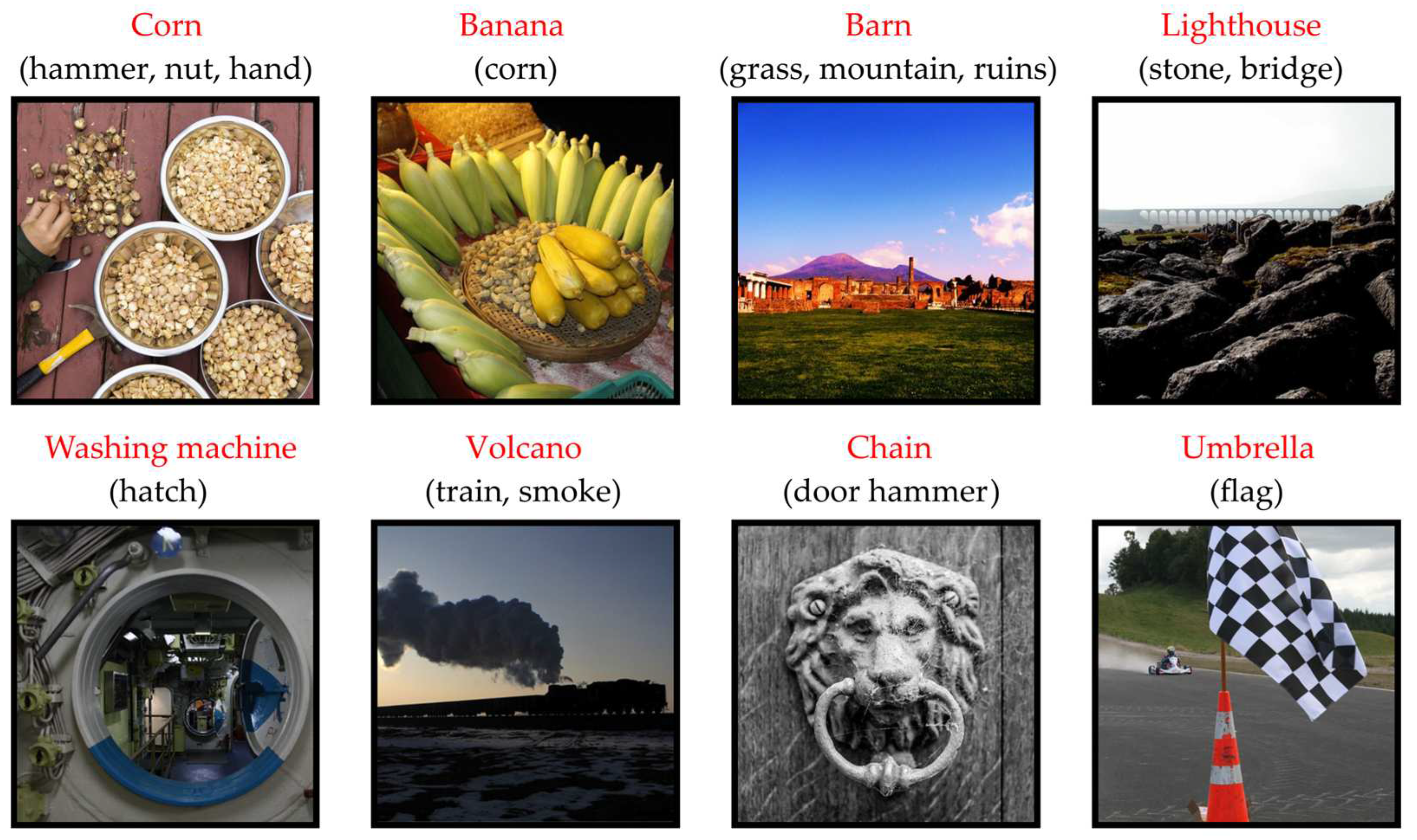
Figure 2.
The essence of the proposed technique.
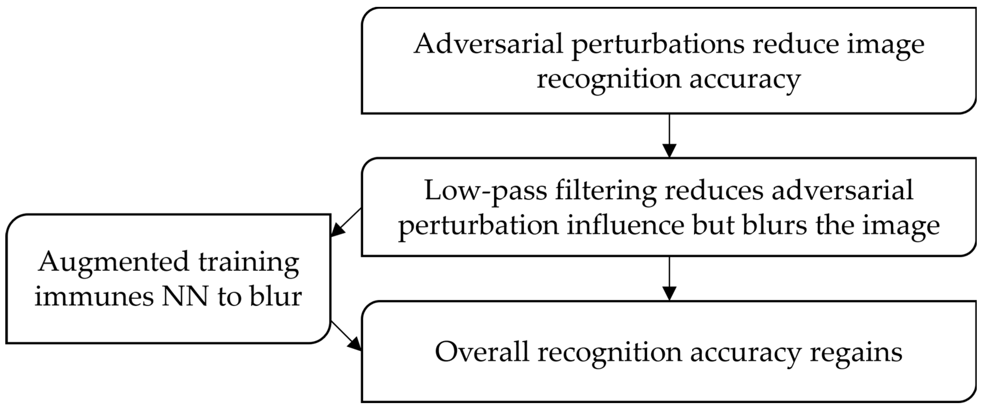
Figure 3.
Image examples from the CIFAR-10 dataset (1 – truck, 2 – ship, 3 – horse, 4 – frog, 5 – dog, 6 – deer, 7 – cat, 8 – bird, 9 – car, 10 – plane).
Figure 3.
Image examples from the CIFAR-10 dataset (1 – truck, 2 – ship, 3 – horse, 4 – frog, 5 – dog, 6 – deer, 7 – cat, 8 – bird, 9 – car, 10 – plane).
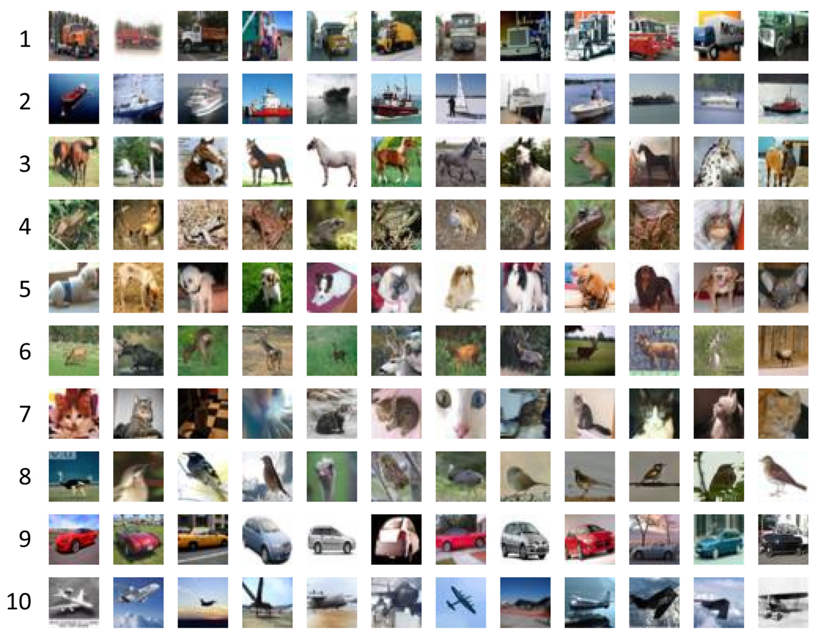
Figure 4.
Image examples from the Natural Images dataset.
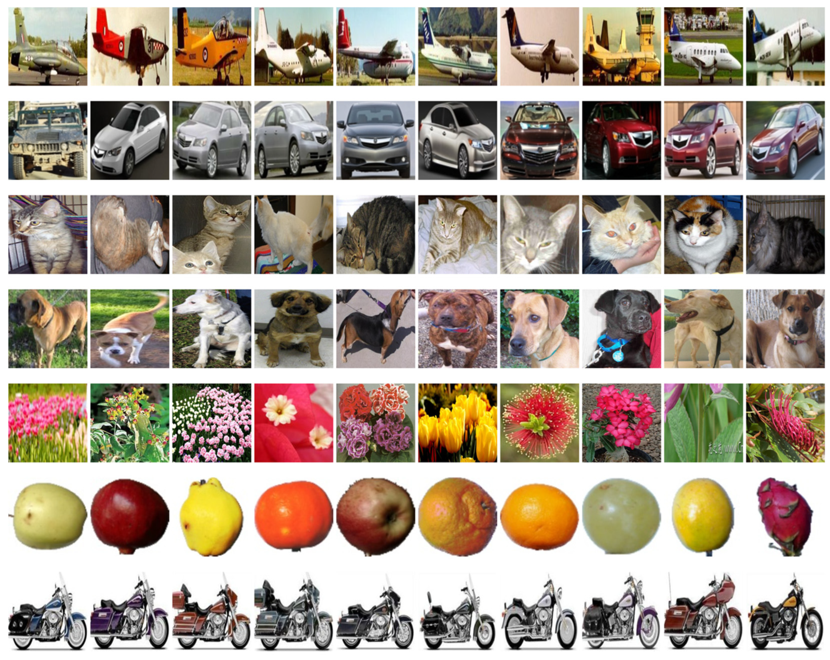
Figure 5.
The architecture of simplified high-speed CNN.
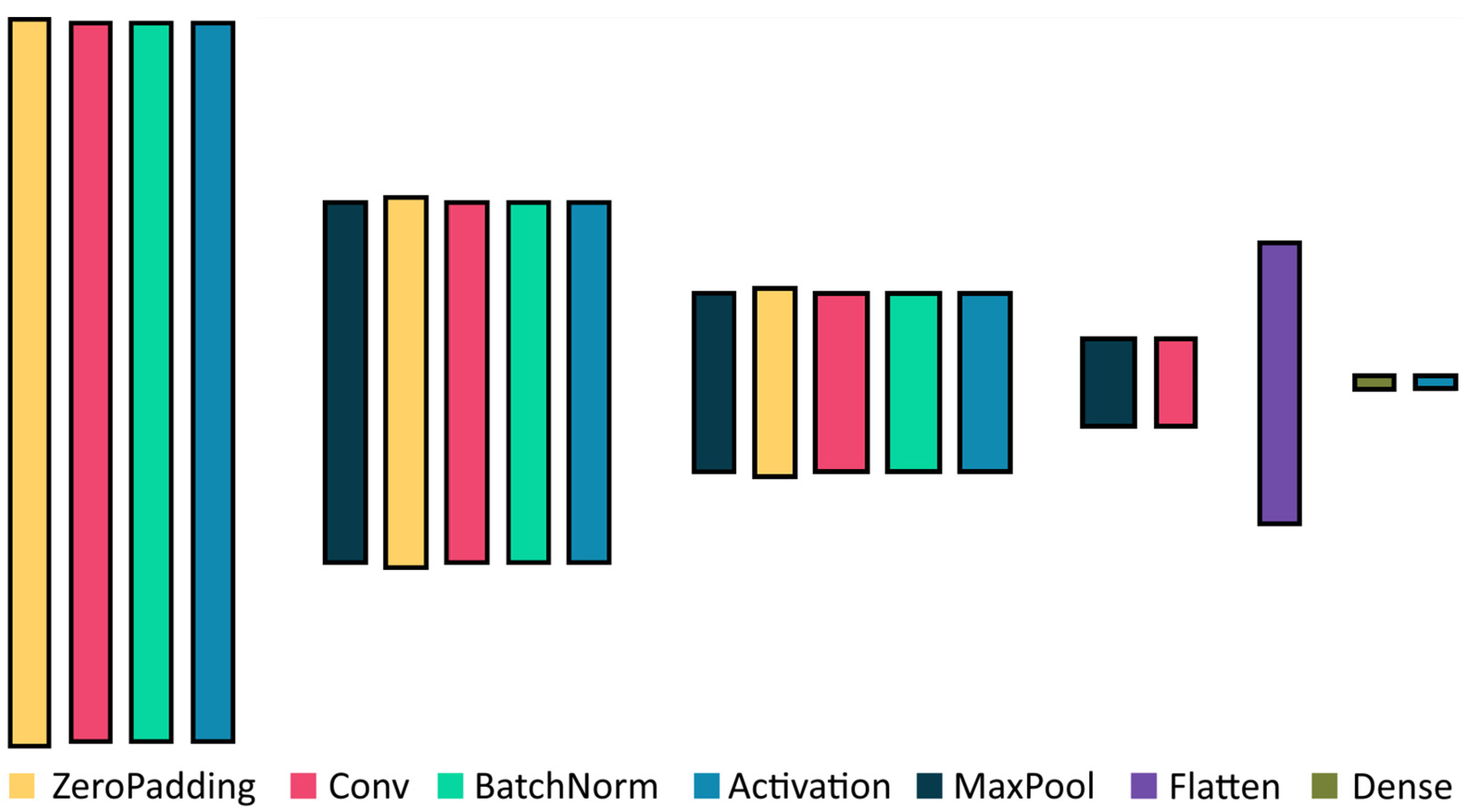
Figure 6.
Effect of FGSM on the recognition accuracy of image datasets (a) Rock-Paper-Scissors Images and (b) Natural Images.
Figure 6.
Effect of FGSM on the recognition accuracy of image datasets (a) Rock-Paper-Scissors Images and (b) Natural Images.
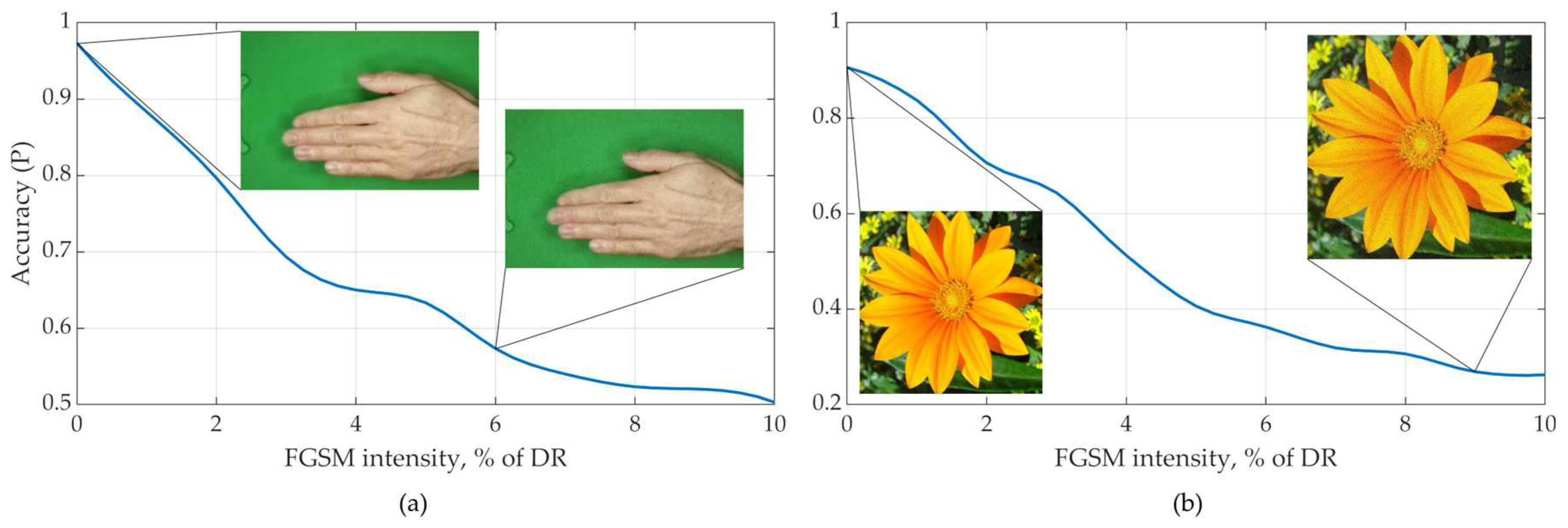
Figure 7.
2-D Fourier transform of image (a) Clean; (b) Clean with FGSM (10%); (c) FGSM; (d) Filtered by Gaussian low-pass filter.
Figure 7.
2-D Fourier transform of image (a) Clean; (b) Clean with FGSM (10%); (c) FGSM; (d) Filtered by Gaussian low-pass filter.

Figure 8.
Mutual energy (scalar product values) of the original image and the attack matrix on Gaussian filter size.
Figure 8.
Mutual energy (scalar product values) of the original image and the attack matrix on Gaussian filter size.
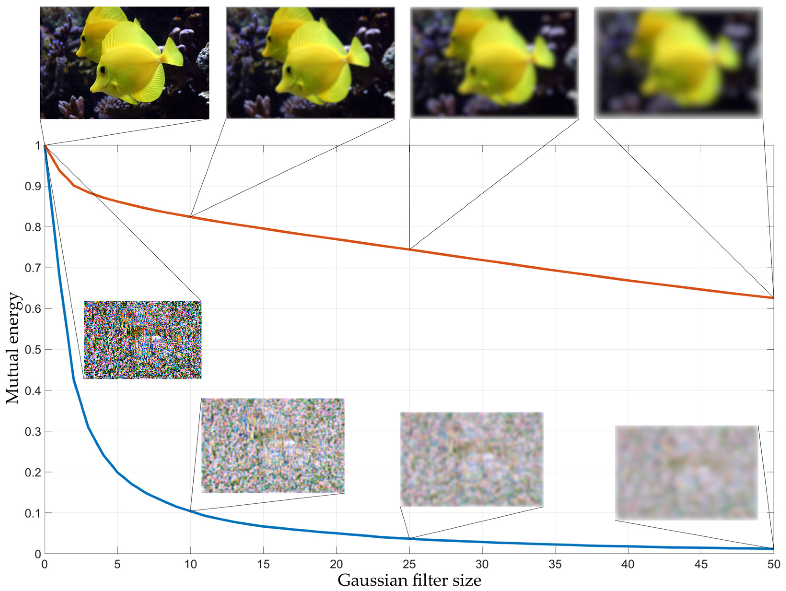
Figure 9.
Algorithm scheme.
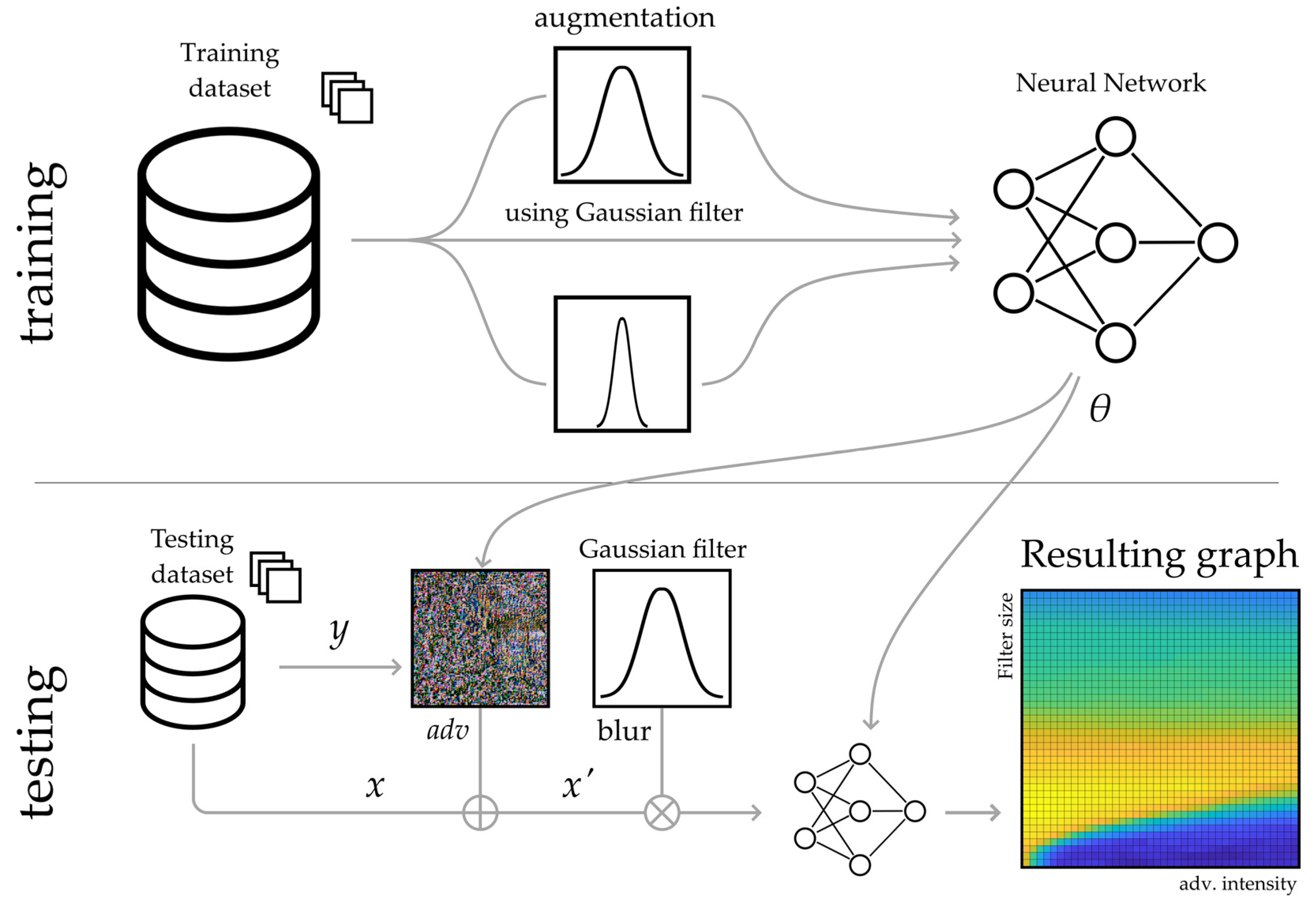
Figure 10.
Accuracy for SimConvNet and Natural Dataset: (a) CNN trained using augmentation with blurred images; (b) No augmentation used.
Figure 10.
Accuracy for SimConvNet and Natural Dataset: (a) CNN trained using augmentation with blurred images; (b) No augmentation used.
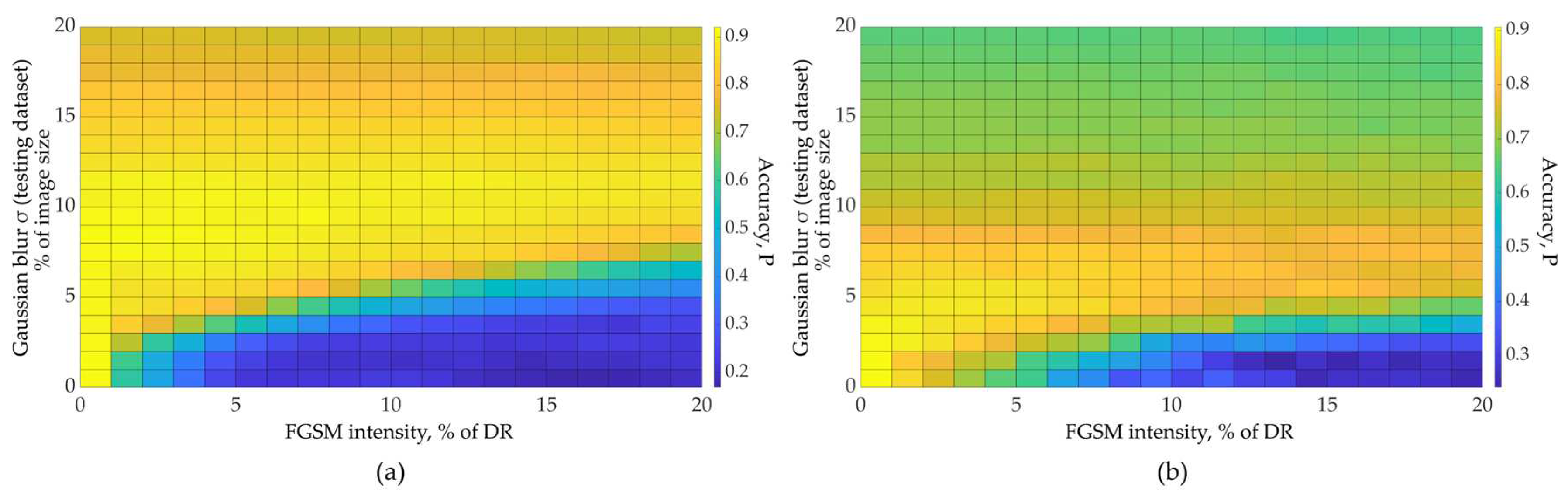
Figure 11.
Accuracy for SimConvNet and Rock-Paper-Scissors Dataset: (a) CNN trained using augmentation with blurred images; (b) No augmentation used.
Figure 11.
Accuracy for SimConvNet and Rock-Paper-Scissors Dataset: (a) CNN trained using augmentation with blurred images; (b) No augmentation used.
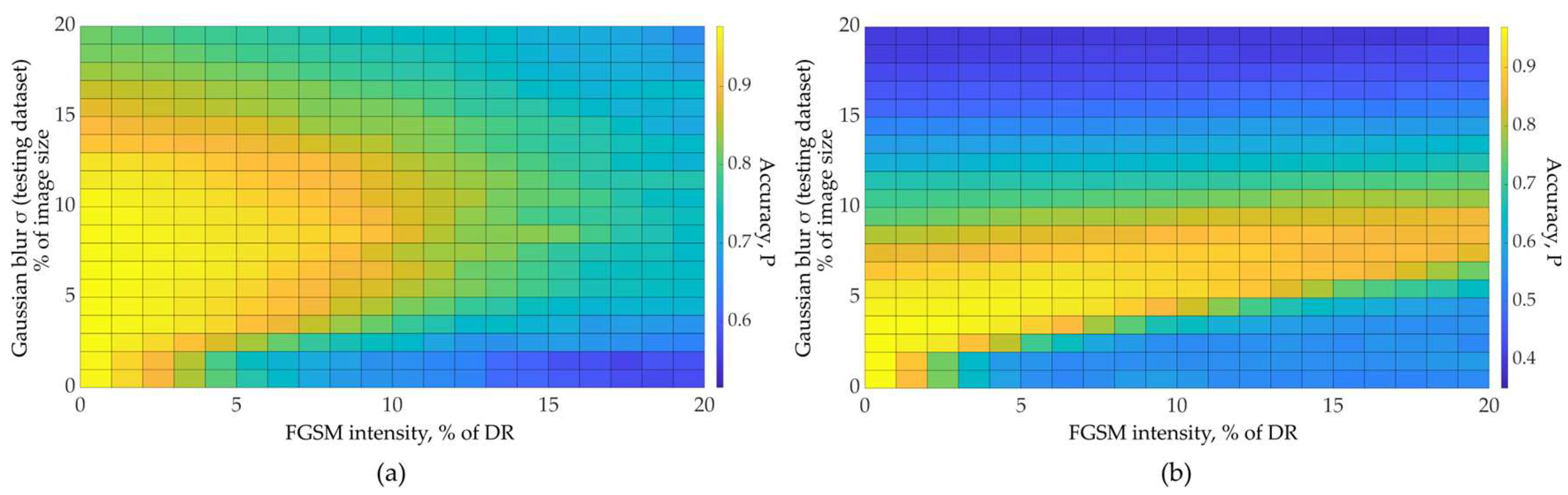
Figure 12.
Accuracy for EfficientNet: (a) Natural Dataset; (b) ImageNet.
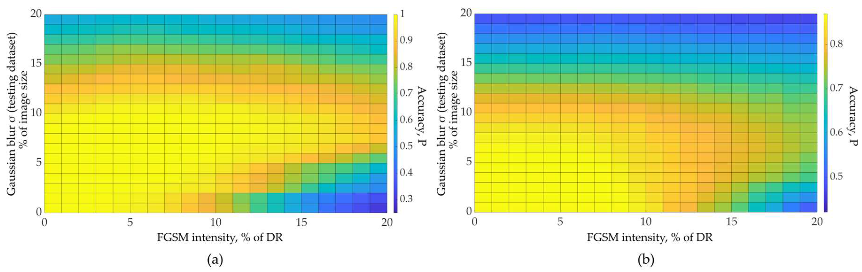

Table 1.
Classification accuracy at various adversarial distortion intensities and possible accuracy gain by applying the filter.
Table 1.
Classification accuracy at various adversarial distortion intensities and possible accuracy gain by applying the filter.
| FGSM intensity | FGSM intensity |
Optimal Low-pass filter size |
Accuracy gain G | ||
|---|---|---|---|---|---|
| SimConvNet (Natural Dataset) |
5 | 0.206 | 0.913 | 10 | 9.1 |
| 10 | 0.206 | 0.9 | 7.9 | ||
| 20 | 0.1875 | 0.894 | 6.7 | ||
| SimConvNet (RPS) |
5 | 0.738 | 0.947 | 8 | 4.9 |
| 10 | 0.66 | 0.879 | 2.8 | ||
| 20 | 0.576 | 0.738 | 1.6 | ||
| EfficientNet (ImageNet) |
15 | 0.699 | 0.781 | 7 | 1.4 |
| 20 | 0.481 | 0.72 | 1.9 | ||
| EfficientNet (Natural Dataset) |
5 | 0.977 | 1 | 7 | ∞ |
| 10 | 0.814 | 0.996 | 46.5 | ||
| 20 | 0.25 | 0.881 | 6.3 |
Disclaimer/Publisher’s Note: The statements, opinions and data contained in all publications are solely those of the individual author(s) and contributor(s) and not of MDPI and/or the editor(s). MDPI and/or the editor(s) disclaim responsibility for any injury to people or property resulting from any ideas, methods, instructions or products referred to in the content. |
© 2023 by the authors. Licensee MDPI, Basel, Switzerland. This article is an open access article distributed under the terms and conditions of the Creative Commons Attribution (CC BY) license (http://creativecommons.org/licenses/by/4.0/).
Copyright: This open access article is published under a Creative Commons CC BY 4.0 license, which permit the free download, distribution, and reuse, provided that the author and preprint are cited in any reuse.


