1. Introduction
Hepatitis B is a severe viral infection that affects the liver, leading to acute and chronic conditions. The virus is commonly transmitted through pregnancy, contact with infected blood or body fluids, and unsafe injections. In 2019, 296 million people lived with chronic hepatitis B, with 1.5 million new infections and an estimated 820,000 deaths, primarily from liver-related complications. Effective vaccines are available that offer essential prevention [
1]. Mathematical modeling is a powerful tool that extensively enriches our comprehension of the complex HBV infection dynamics and the consequential effects of antiviral therapies. Classical models of HBV infection dynamics are typically anchored in ordinary differential equations (ODEs), reflecting the intricate interactions between the virus and the host immune response [
2,
3,
4,
15,
17,
26].
Although these deterministic models provide pivotal insights into HBV’s pathogenesis and therapeutic interventions’ impacts, they tend to neglect the inherent randomness and variability intrinsic to biological processes. This aspect can be critically important, particularly in shaping the infection dynamics [
5]. Therefore, stochastic models have been suggested to offer a more nuanced and accurate representation of HBV dynamics. These models embed random variability into the equations, thereby encapsulating fluctuations in viral and cellular populations and the uncertainty associated with parameters such as infection rates and immune responses [
6,
7].
One of the first works to provide valuable insight into the nature of the infection and treatment effects are deterministic models, mainly based on ordinary differential equations (ODEs) [
2,
3,
4]. These models represent the virus-host immune response interaction, capturing the core dynamics of the infection.
However, deterministic models’ primary limitation is their inability to consider the inherent variability in biological processes [
5,
42]. This variability can be integral to understanding the dynamics of infection, including fluctuations in viral and cellular populations and uncertainty in parameters such as infection rates and immune responses.
Recently, stochastic models have been suggested to tackle this limitation and provide a more realistic representation of the HBV infection dynamics [
6,
7]. These models incorporate random variations into the system, thus accounting for the variability inherent in biological processes.
This research presents a mathematical analysis of the stochastics HBV infection dynamics model. The existence, uniqueness, and probability of the solution are discussed then we studied the local and global stability, where we show the necessary and sufficient conditions of stability in probability. In addition, we show the existence of ergodic stationary distributions. To validate our theoretical findings, we substantiate the results with numerical simulations, offering a robust and practical tool for understanding the complex behavior of HBV dynamics.
2. Introduction
Hepatitis B is a severe viral infection that affects the liver, leading to acute and chronic conditions. The virus is commonly transmitted through pregnancy, contact with infected blood or body fluids, and unsafe injections. In 2019, 296 million people lived with chronic hepatitis B, with 1.5 million new infections and an estimated 820,000 deaths, primarily from liver-related complications. Effective vaccines are available that offer essential prevention [
1]. Mathematical modeling is a powerful tool that extensively enriches our comprehension of the complex HBV infection dynamics and the consequential effects of antiviral therapies. Classical models of HBV infection dynamics are typically anchored in ordinary differential equations (ODEs), reflecting the intricate interactions between the virus and the host immune response [
2,
3,
4,
15,
17,
26].
Although these deterministic models provide pivotal insights into HBV’s pathogenesis and therapeutic interventions’ impacts, they tend to neglect the inherent randomness and variability intrinsic to biological processes. This aspect can be critically important, particularly in shaping the infection dynamics [
5]. Therefore, stochastic models have been suggested to offer a more nuanced and accurate representation of HBV dynamics. These models embed random variability into the equations, thereby encapsulating fluctuations in viral and cellular populations and the uncertainty associated with parameters such as infection rates and immune responses [
6,
7].
One of the first works to provide valuable insight into the nature of the infection and treatment effects are deterministic models, mainly based on ordinary differential equations (ODEs) [
2,
3,
4]. These models represent the virus-host immune response interaction, capturing the core dynamics of the infection.
However, deterministic models’ primary limitation is their inability to consider the inherent variability in biological processes [
5,
42]. This variability can be integral to understanding the dynamics of infection, including fluctuations in viral and cellular populations and uncertainty in parameters such as infection rates and immune responses.
Recently, stochastic models have been suggested to tackle this limitation and provide a more realistic representation of the HBV infection dynamics [
6,
7]. These models incorporate random variations into the system, thus accounting for the variability inherent in biological processes.
This research presents a mathematical analysis of the stochastics HBV infection dynamics model. The existence, uniqueness, and probability of the solution are discussed then we studied the local and global stability, where we show the necessary and sufficient conditions of stability in probability. In addition, we show the existence of ergodic stationary distributions. To validate our theoretical findings, we substantiate the results with numerical simulations, offering a robust and practical tool for understanding the complex behavior of HBV dynamics.
3. Model Formulation
Our research employs a modified stochastic version of a deterministic model that represents the dynamics of HBV infection.
The deterministic model [
42] is presented by the following system of ordinary differential equations (ODEs):
The parameters in these equations are defined in
Table 1.
The stochastic model, built upon the deterministic model, adds stochastic noise to each equation to capture the inherent variability in biological systems:
Here, , , and represent standard Wiener processes, and , , and represent the noise coefficients that control the amplitude of the stochastic fluctuations.
The system (
2) can be reformulated in the following way:
Here, the initial condition is , and is represented as a vector .
The functions
and
, along with the differential
, are defined as follows:
3.1. Preliminaries
Before exploring the solution properties and the stability analysis of the stochastic system
2, it is essential to establish a foundation by defining some pertinent terms and theories. These concepts, drawn from [
18], lay the groundwork for the forthcoming analysis.
In general, equation
3 can be reformulated as a stochastic equation of d dimension within the context of a complete probability space
, paired with a filter
. This reformulation can be expressed as
Here,
and
are Borel measurable, and the white noise
, for
. Assuming that
and that the initial value
is
-measurable
random variable such that
, equation
4 can be recognized as an Itô type stochastic differential equation.
Definition 1. A stochastic process in is identified as a solution of equation 4 if it satisfies the following conditions:
-
i.
is continuous and -adapted;
-
ii.
and ;
-
iii.
equation 4 is valid for every with probability 1.
A solution is deemed unique if any other solution fulfills the following condition:
Lemma 1.
For any , the following inequality holds.
Proof. The proof is straightforward since the function has a minimum at . □
A d-dimensional stochastic equation can, in general, be expressed as
Where with the initial condition , and W(t) is the m-dimensional white noise defined on a complete probability space .
3.2. Itô’s Formula
We define a differential operator
L as follows:
Consider
, a nonnegative twice differentiable function defined on
, applying operator
on
V, we get:
where
,
, and
.
Therefore, the Itô formula can be defined as:
In the next section, we will discuss the properties of the solution to the system given by Eq. (
2).
3.3. Properties of Solution
We discuss the solution properties of the system
2, such as existence, uniqueness, and positivity. The dynamics of a population model can be understood by demonstrating that the solution is global and positive for all time
. The coefficients of the above stochastic system are locally Lipschitz and satisfy the linear growth condition [
12].
Theorem 1. For any initial value , there exists a unique solution to the system (2) for all . Furthermore, this solution remains positive for all with probability 1, i.e., for all almost surely.
Proof. The coefficients of the equations (
2) are continuous and locally Lipschitz. Thus, there is a unique local solution
for any initial
, where
. To establish that the solution is global, we must show that
almost surely.
Choose
large enough such that
, and let
. Define
We must show that
is an empty set, assuming that
. Since
is an increasing sequence, let
. By definition,
a.s.
To complete the proof, we must show that
a.s., which implies
. Assume by contradiction that this is not true. Then there exists a pair of constants
and
such that
, which implies the existence of an integer
such that
Now, let’s define a function
:
which is non-negative due to the inequality
(see [
19]). By applying Itô’s formula on
, we get the following:
which simplifies to
where
, and
.
Let
. Integrating the above inequality, if
we get
By definition, this implies
From the Gronwall inequality, we obtain the following.
We then set
for
and, by inequality
9,
. Note that there exist some
or
z such that
or
, for every
. Therefore,
is greater than
and
, i.e.,
From the inequalities
9 and
10, we obtain
where
is the indicator function of
. Taking the limit as
n approaches
∞ yields
, which is a contradiction. Therefore,
a.s., which completes the proof. □
4. Stability Analysis
This section is dedicated to the exploration of the stability analysis of the system (
2). For this discussion, we will revisit some requisite definitions and theorems. For further details, see [
18] and [
13].
Definition 2
-
(i)
-
The trivial solution of equation 4 is deemed stable in probability if, given any and , there exists a such that
whenever . If not, it is termed stochastically unstable.
-
(ii)
-
The trivial solution is considered stochastically asymptotically stable if it is stochastically stable and, for each and , there exists a such that
whenever .
-
(iii)
The trivial solution is designated as stochastically asymptotically stable in the large if it is stochastically stable and, additionally, for all and , there is a such that
-
(iv)
-
The trivial solution of equation 4 is characterized as almost surely exponentially stable if
for all .
Observe that the first equation of our system,
2, does not possess a direct equilibrium point in
. However, the second and the third equations of the system
2 have a common equilibrium point at
.
The forthcoming theorem will demonstrate that the trivial solution is stable. For now, let us concentrate on variables. We will return to the equation later to demonstrate that it is stable in distribution. The upcoming theorem asserts that and are exponentially stable under certain conditions.
Theorem 2. In the system 2, and are almost surely exponentially stable if and only if the following conditions are met
-
a.
-
b.
where .
The proof proceeds as follows.
Proof. By adding equations
and
equations, we get
Let
for
. Applying Itô’s formula, we have
Assuming the conditions of the theorem are met, then the matrix
is negative-definite, which implies it has at least one negative eigenvalue. Let
denote the largest eigenvalue. With this, the inequality above can be expressed as:
By utilizing the inequality
, it follows that
, yielding:
By integrating the inequality above and applying the fact from [
18] that
we derive
This concludes the proof. □
Remark 1. The stability of components y and z has been achieved without reliance on the reproductive number , irrespective of whether or . Moreover, it is crucial to note that the conditions within theorem 2 cannot hold in the deterministic case when both .
We aim to demonstrate the initial component stability. We aim to prove that is stable in distribution, which implies that it is stable around the mean value . However, before proceeding, let’s first introduce some necessary lemmas.
Lemma 2.
Assume is a one-dimensional standard Brownian motion. Then, the expectation is given by
Proof. Define
. By the definition of Brownian motion, we know that
. Hence,
□
Lemma 3.
Assume that is a solution to
Then, we have for any initial .
Proof. Given an initial value
, there is a unique solution
to equation (
11) with the explicit form
Applying the expectation to the above equation and using the fact that
, we get
By applying lemma 2, we find
□
Lemma 4. Assume that is a solution of equation 11. Then, for any initial value , we obtain the following results:
-
i.
admits a unique stationary distribution π, where represents the Gamma function.
-
ii.
satisfies the equation
Proof.
- i.
-
Define
, a twice continuously differentiable function. Applying the It
formula, we have
By choosing a sufficiently small
and defining
, we find that
This completes the first part of the proof.
- ii.
-
Employing the ergodicity of
, we obtain
Therefore,
where we used the fact
□
Theorem 3.
Assume to be a solution of the system 2, and to be a solution of equation 11. Under the condition of theorem 2, we can confirm that
Proof. By leveraging the comparison theorem of stochastic differential equations, we can assert that
, i.e.,
To conclude this proof, it is crucial to demonstrate that
a.s.
We now introduce a stochastic differential equation, which will assist us in this proof:
where the initial condition is
.
Recall
in the system
2,
and equation
11,
From fact that
We will proceed to prove the following claims.
claim 1:
almost surely.
Proof. Subtracting the given equations, we find
This yields a solution.
where
By Theorem 2, we know that
and
almost surely as
. Therefore,
for all
and
. Therefore,
where
Given
and
almost surely, we conclude
□
claim 2
a.s.
Proof. Beginning with the first equation in the system
2 and
11, we can write
which leads to the solution
analog cognize
as the solution for equation
14, which can be expressed explicitly as
Hence,
Applying the expectation and invoking lemma 2, we find
Additionally, we know
which implies
Therefore,
□
With
13,
15, and
16, we conclude the proof of the theorem.
4.1. Existence of Ergodic Stationary Distribution
Let
be a Markov process in
represented by the following stochastic differential equations:
The diffusion matrix is defined as
Lemma 5.(See [38,39]) The model in Equation 17 is positive recurrent if there exists a boundary open subset with a regular boundary and the following conditions hold:
-
(A1)
There is a positive number M such that
-
(A2)
-
There exists a nonnegative -function such that for some , and any . Moreover, the positive recurrent process has a unique stationary distribution , and
for all , where is an integrable function with respect to the measure .
Theorem 4.
Assume that . Under the conditions , , and , the system 2 has a unique ergodic stationary distribution .
Proof. We have seen that the system
2 has a unique positive solution
for any initial value
.
The diffusion matrix of the system is given by
Then
where,
, thus condition
satisfied.
We want to show that condition is also satisfied by constructing a nonnegative Lyapunov function V such as .
Consider the positive functions
Now let
By applying It
formula we get
since we have
, then we get
By using the fact that,
, we get
thus
where
, and since
, then
Similarly,
Thus,
where
,
,
, and
Since
are positive and by the same computation as in [
40], we obtained
then the ellipsoid
lies entirely in
, so we can take any neighborhood
D of this ellipsoid, such that
Therefore, condition (A2) also holds and completes the proof. □
5. Numerical Solution
Numerous numerical methods exist for solving stochastic dynamical systems. Some prominent techniques include the Euler-Maruyama Method, Milstein Method, Stochastic Runge-Kutta Methods, Strong and Weak Taylor Methods, Split-Step Methods, Stochastic Theta Method, Multilevel Monte Carlo Methods, Gaussian Process Emulators, Stochastic Collocation and Galerkin Methods, Particle Filters, and Hybrid Methods. This study considers only the Euler-Maruyama and Milstein methods.
Euler-Maruyama method: As one of the simplest numerical methods for SDEs, the Euler-Maruyama method extends the deterministic Euler method to the stochastic context [
9]. Despite its simplicity and ease of implementation, the method only provides strong convergence of order
.
Milstein method: The Milstein method improves upon the Euler-Maruyama method by including additional terms in the Taylor series expansion of the SDE. This method provides a strong convergence of order
under suitable conditions, doubling the convergence rate of the Euler-Maruyama method [
10].
These methods and many others provide a rich toolbox for the numerical solution of SDEs. The choice of method depends on several factors, such as the specific form of the SDE, the regularity of its coefficients, and the desired balance between accuracy and computational cost. For our model
3, we will solve it numerically using the Euler-Maruyama and Milstein methods as follows.
Euler-Maruyama Method
To solve the stochastic model numerically, we use the Euler-Maruyama scheme, a stochastic analog of the well-known Euler method for ordinary differential equations. The system gives the stochastic model to be solved (
2). The Euler-Maruyama scheme for system (
2) can be described as follows:
Discretize the time domain into n intervals of size , where . Denote , , and by , , and respectively.
Initialize , and as the initial conditions.
For each time step , compute the increments , , and
Update the solution from time
to
as follows
This procedure gives a numerical approximation of the solution to the stochastic differential equations in the system (
2). To implement this scheme, one needs to generate increments
,
, and
, normally distributed random numbers with mean 0 and variance
.
5.1. Milstein Method
The Milstein method is another widely used numerical approach to solving stochastic differential equations, which extends the Euler-Maruyama method by including an additional term to account for the diffusion term in the stochastic system.
The scheme for system (
2) using the Milstein method can be detailed as follows:
As in the Euler-Maruyama method, discretize the time domain into n intervals of size and initialize , , and as the initial conditions.
For each time step , calculate the increments , , and in the same way as the Euler-Maruyama method.
Update the solution from time
to
by
This approach considers the second moment of the diffusion term, thereby providing more accurate approximations of the solution of the stochastic system (
2). The implementation involves a similar procedure to the Euler-Maruyama method but with additional terms to be computed at each step.
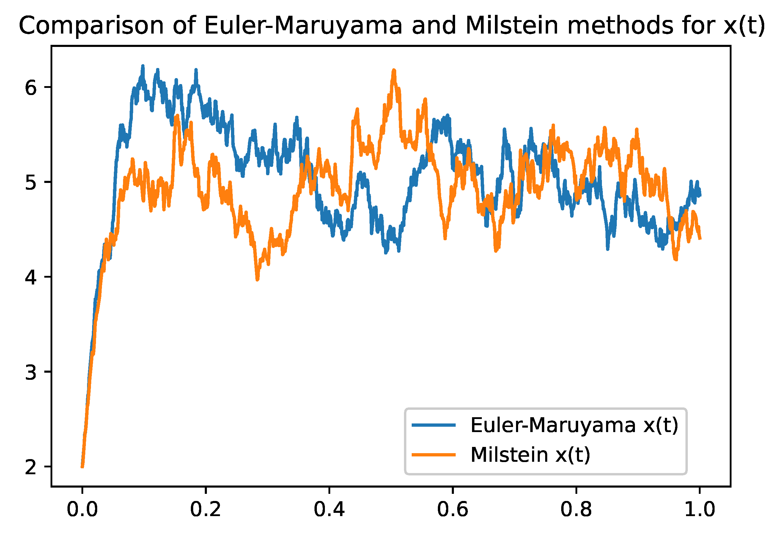
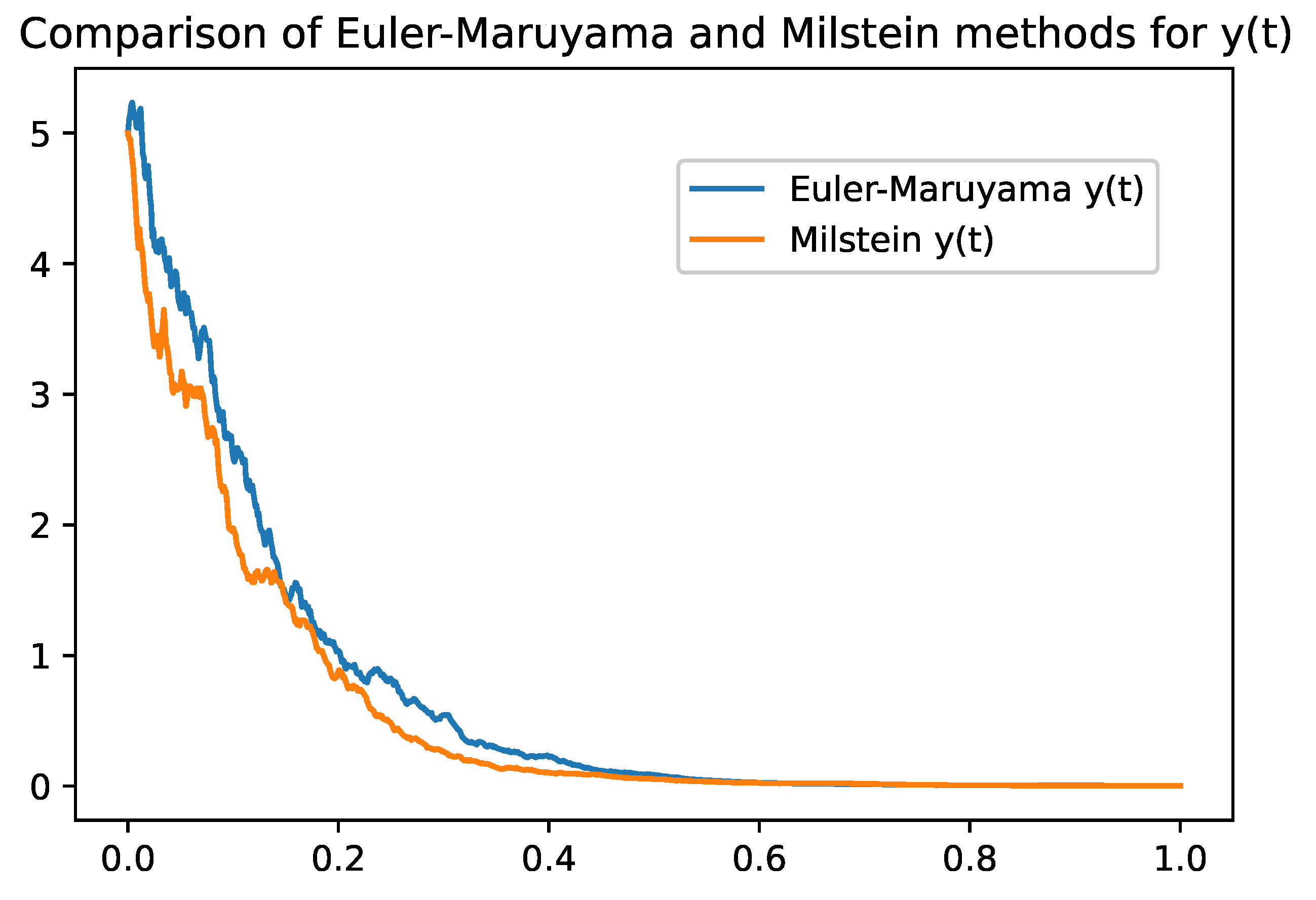
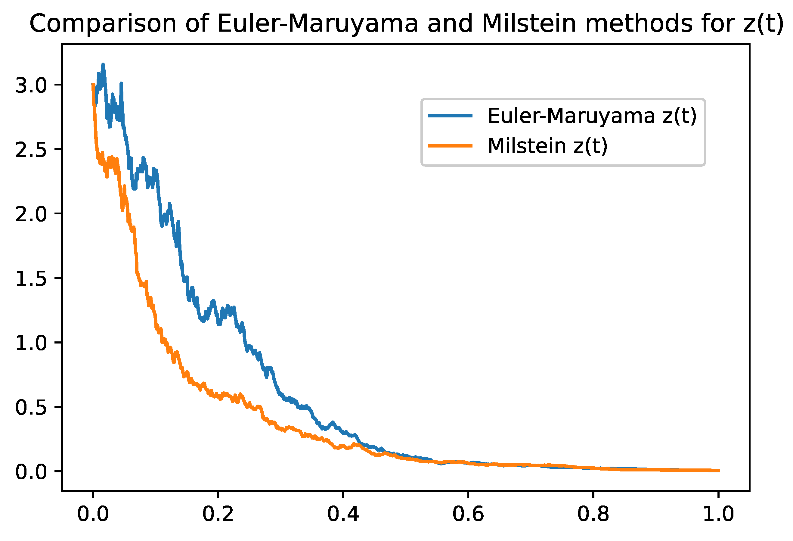
Omparison between Euler-Maruyama and Milstein Methods
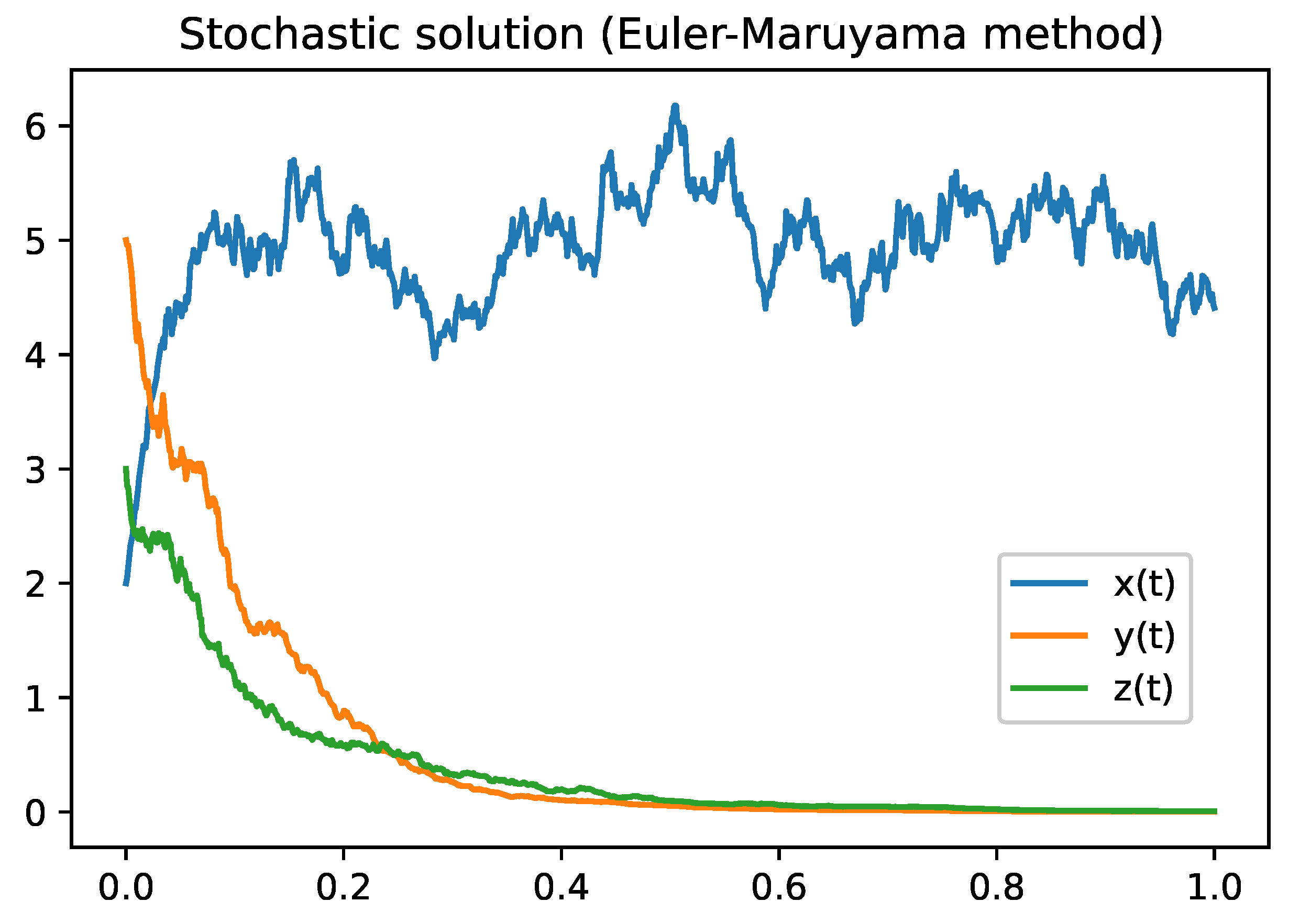
Figure 1.
Figure describes the solution of the model
2 using Euler-Maruyama Method. Parameter values are defined in the
Table 3
Figure 1.
Figure describes the solution of the model
2 using Euler-Maruyama Method. Parameter values are defined in the
Table 3
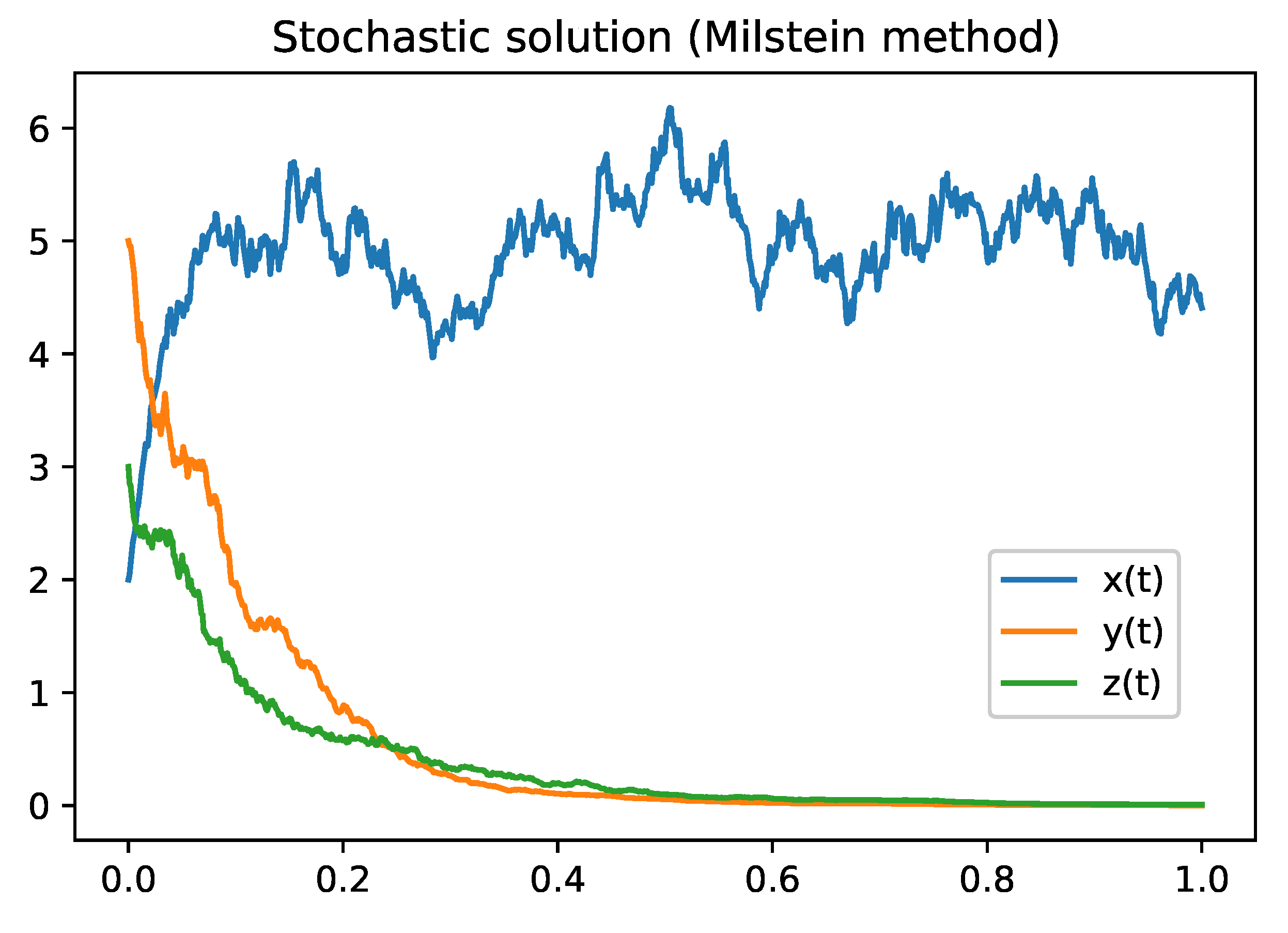
Figure 2.
Figure describes the solution of the model
2 using Milstein Method. Parameter values are defined in the
Table 3
Figure 2.
Figure describes the solution of the model
2 using Milstein Method. Parameter values are defined in the
Table 3
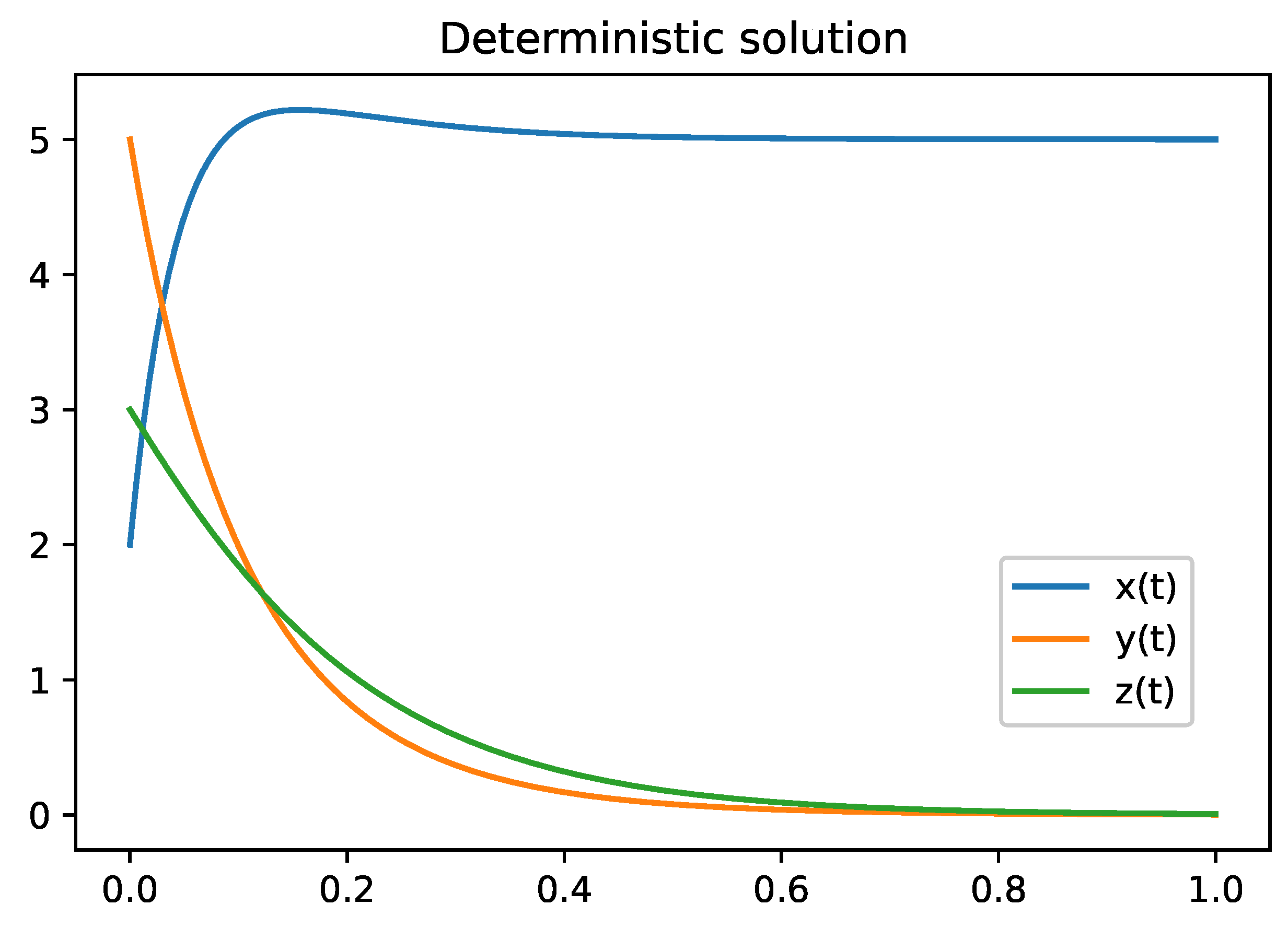
Figure 3.
Figure describes the deterministic solution of the model
2. Parameter values are defined in the
Table 3
Figure 3.
Figure describes the deterministic solution of the model
2. Parameter values are defined in the
Table 3
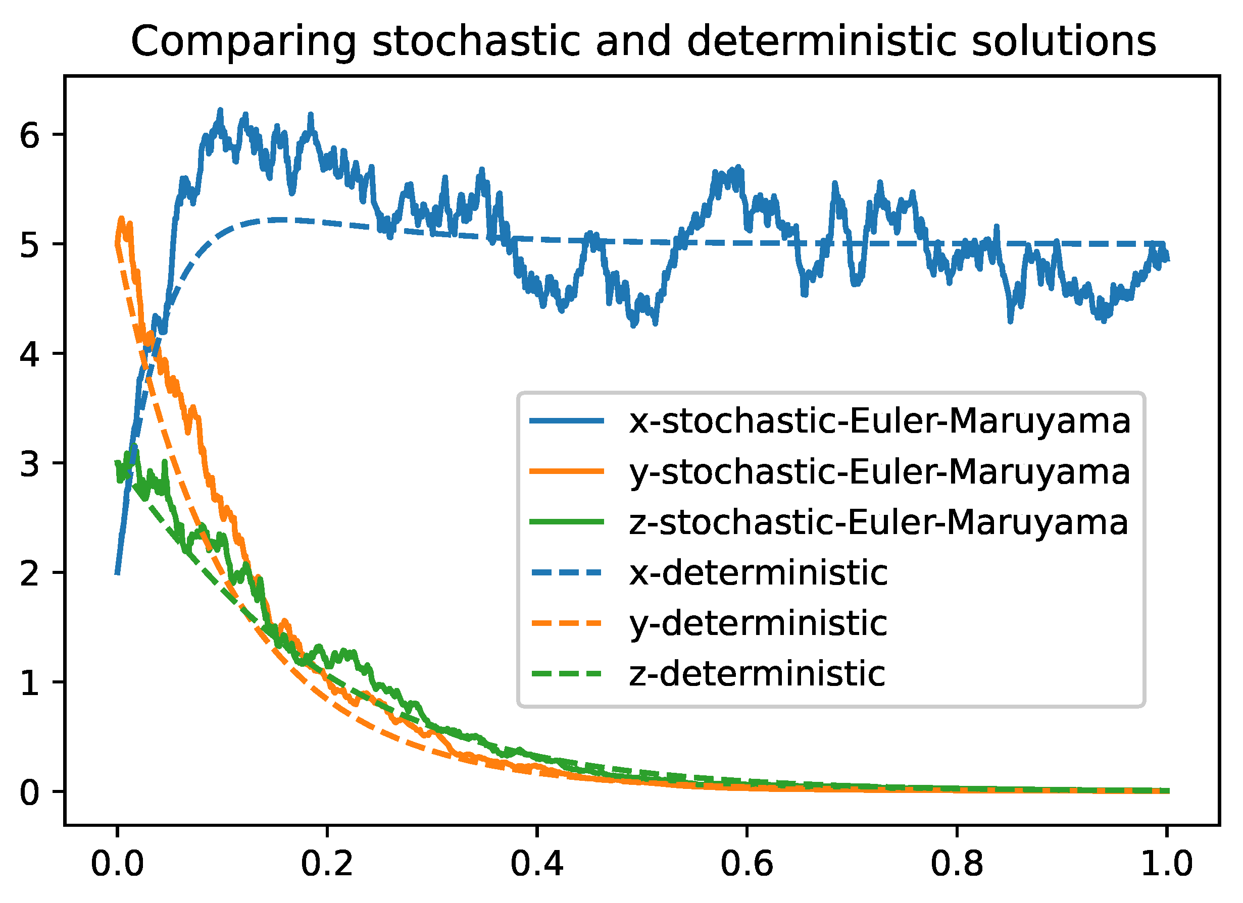
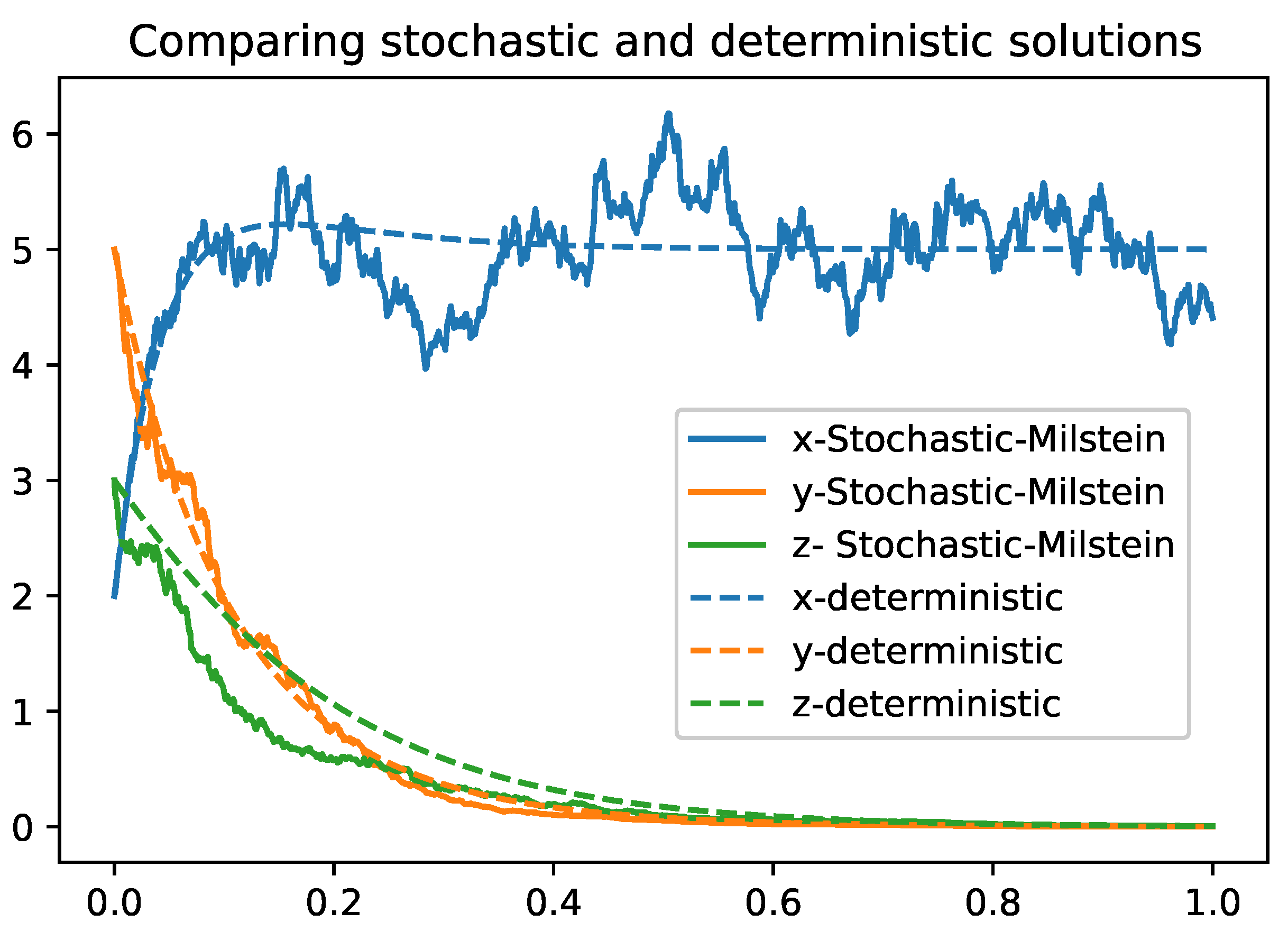
Figure 4.
Figure compares the stochastic "Euler-Maruyama" and deterministic solutions. Parameter values are defined in the
Table 3
Figure 4.
Figure compares the stochastic "Euler-Maruyama" and deterministic solutions. Parameter values are defined in the
Table 3
Figure 5.
Figure compares the stochastic " Milstein" and deterministic solutions. Parameter values are defined in the
Table 3
Figure 5.
Figure compares the stochastic " Milstein" and deterministic solutions. Parameter values are defined in the
Table 3
Figure 6.
Figure compares the stochastic " Milstein" and deterministic solutions. Parameter values are defined in the
Table 3
Figure 6.
Figure compares the stochastic " Milstein" and deterministic solutions. Parameter values are defined in the
Table 3
Figure 7.
Figure compares the stochastic " Milstein" and deterministic solutions. Parameter values are defined in the
Table 3
Figure 7.
Figure compares the stochastic " Milstein" and deterministic solutions. Parameter values are defined in the
Table 3
Figure 8.
Figure compares the stochastic " Milstein" and deterministic solutions. Parameter values are defined in the
Table 3
Figure 8.
Figure compares the stochastic " Milstein" and deterministic solutions. Parameter values are defined in the
Table 3
Table 2 summarizes the main differences between the two methods, highlighting the trade-offs between simplicity, computational cost, accuracy, and stability. Both methods provide valuable tools for numerically solving stochastic models and can be chosen according to the specific needs and constraints of the problem.
6. Conclusion
This paper presents a refined stochastic model for Hepatitis B Virus (HBV) infection dynamics, capturing biological processes’ inherent variability and randomness. By introducing preliminary concepts, the study fosters easy comprehension, paving the way for an analysis that ensures the solution’s existence, uniqueness, and positive for all positive initial values.
The stability analysis of the model is explored, delineating necessary and sufficient conditions for stability in probability. This contributes to a more profound understanding of the dynamics of HBV infection and is a robust foundation for further investigation.
The study employs two distinguished numerical methods, Euler-Maruyama and Milstein, to solve the stochastic differential equations in the system (
2). While the Euler-Maruyama method provides a simple solution with a lower convergence rate, the Milstein method enhances accuracy and stability by accounting for the second moment of the diffusion term. These numerical simulations corroborate the theoretical findings and illustrate the practical applicability of the model.
Despite certain limitations, this research marks a significant advance in the field of HBV infection dynamics. It offers a deeper understanding of the subject and encourages progress toward devising effective strategies for control and prevention. The insights gained from this study serve as a vital stepping stone for future explorations in this critical area of public health.
Conflicts of Interest:
Declare conflicts of interest or state “The authors declare no conflict of interest.” Authors must identify and declare any personal circumstances or interests that may be perceived as inappropriately influencing the representation or interpretation of reported research results. Any role of the funders in the design of the study; in the collection, analysis, or interpretation of data; in the writing of the manuscript; or in the decision to publish the results must be declared in this section. If there is no role, please state “The funders had no role in the design of the study; in the collection, analyses, or interpretation of data; in the writing of the manuscript; or in the decision to publish the results”.
References
- World Health Organization, Hepatitis B, 2023, https://www.who.int/news-room/fact-sheets/detail/hepatitis-b, Accessed: 2023-07-23.
- Nowak, Martin A. and others, Viral dynamics of primary viremia and antiretroviral therapy in simian immunodeficiency virus infection, Journal of Virology, vol. 70, no. 10, pp. 6735–6741, 1996, Am Soc Microbiol. [CrossRef]
- Bangham, Charles R., Population dynamics of immune responses to persistent viruses, Science, vol. 272, no. 5258, pp. 74–79, 1996, American Association for the Advancement of Science. [CrossRef]
- Perelson, Alan S. and Nelson, Patrick W., Modelling viral and immune system dynamics, Nature Reviews Immunology, vol. 2, no. 1, pp. 28–36, 2002, Nature Publishing Group.
- Lloyd, Alun L., Realistic distributions of infectious periods in epidemic models: Changing patterns of persistence and dynamics, Theoretical Population Biology, vol. 60, no. 1, pp. 59–71, 2001, Elsevier. [CrossRef]
- Ribeiro, Andre S., Effects of stochastic population dynamics on the quantification of gene expression, Physical Review E, vol. 71, no. 1, pp. 011912, 2005, APS.
- Guedj, Jeremie and Perelson, Alan S., Modeling shows that the NS5A inhibitor daclatasvir has two modes of action and yields a shorter estimate of the hepatitis C virus half-life, Proceedings of the National Academy of Sciences, vol. 110, no. 10, pp. 3991–3996, 2013, National Academy of Sciences. [CrossRef]
- Gardiner, Crispin, Handbook of stochastic methods: for physics, chemistry and the natural sciences, 2004, Springer Science & Business Media.
- Kloeden, Peter E. and Platen, Eckhard, Numerical solution of stochastic differential equations, 2013, Springer Science & Business Media.
- Higham, Desmond J., Algorithmic introduction to numerical simulation of stochastic differential equations, SIAM review, vol. 43, no. 3, pp. 525–546, 2001, SIAM. [CrossRef]
- Rackauckas, Christopher and Nie, Qing, Adaptive methods for stochastic differential equations via natural embeddings and rejection sampling with memory, Discrete and continuous dynamical systems. Series B, vol. 22, no. 7, pp. 2731–2761, 2017, American Institute of Mathematical Sciences. [CrossRef]
- Has’minskii, R. Z., Stochastic Stability of Differential Equations, 1980, Sijthoff Noordhoff, Alphen aan den Rijn, The Netherlands. [CrossRef]
- Caraballo, Tomas and Han, Xiaoying, Applied Nonautonomous and Random Dynamical Systems, 2016, SpringerBriefs. [CrossRef]
- arXiv:2305.08210, 2023.Alsammani, Abdallah, Mathematical Analysis of Autonomous and Nonautonomous Hepatitis B Virus Transmission Models, arXiv preprint arXiv:2305.08210, 2023.
- Alsammani, Abdallah Alhadi Mahadi, Dynamical Behavior of Nonautonomous and Stochastic HBV Infection Model, Ph.D. thesis, Auburn University, 2020.
- Nowak, Martin A. and others, Viral dynamics in hepatitis B virus infection, Proceedings of the National Academy of Sciences, vol. 93, no. 9, pp. 4398–4402, 1996.
- Payne, R.J.H. and Nowak, M.A. and Blumberg, B., The dynamics of hepatitis B virus infection, Proc. Natl. Acad. Sci. USA, vol. 93, pp. 6542–6546, 1996.
- Mao, X., Stochastic Differential Equations and Applications, 2nd ed., Horwood Publishing Limited, 2007.
- Dalal, N. and Greenhalgh, D. and Mao, X., A Stochastic Model for Internal HIV Dynamics, Journal of Mathematical Analysis and Applications, 2008.
- Hui, H. and Nie, L., Analysis of a Stochastic HBV Infection Model with Nonlinear Incidence Rate, Journal Of Biological Systems, vol. 27, no. 3, 2019. [CrossRef]
- Smith, Hall L., Monotone Dynamical Systems, AMS, 1995. [CrossRef]
- Leenheer, Patric DE and Smith, Hall L., Virus Dynamics: a Global Analysis, SIAM J. Appl Math, vol. 63, no. 4, 2003. [CrossRef]
- Nowak, Martin A. and Bangham, Charles R.M., Population Dynamics of Immune Responses to Persistent Viruses, Science, vol. 271, pp. 74–79, 1996. [CrossRef]
- Nowak, Martin A. and Bangham, Charles R.M., Virus Dynamics, Oxford University Press, 2000.
- Perelson, A.S. and Nelson, P.W., Mathematical analysis of HIV-1 dynamics in vivo, SIAM Rev., vol. 41, pp. 3–44, 1999. [CrossRef]
- Abdulrashid, I. and Alsammani, A. and Han, X., Stability Analysis of Chemotherapy Model with Delays, Discrete and Continuous Dynamical Systems Series B, vol. 24, 2019. [CrossRef]
- Perelson, A.S. and Neumann, A.U. and Markowitz, M. and Leonard, J.M. and Ho, D.D., HIV-1 dynamics in vivo: virion clearance rate, infected cell life-span, and viral generation time, Science, vol. 271, pp. 1582–1586, 196. [CrossRef]
- Gourley, S.A. and Kuang, Y. and Nagy, J.D., Dynamics of a delay differential model of hepatitis B virus infection, J. Biological Dynamics, vol. 2, pp. 140–153, 2008. [CrossRef]
- Lewin, S.R. and Riberiro, R.M. and Walters, T., and others, Analysis of Hepatitis B viral load decline under potent therapy: Complex decay profiles observed, Hepatology, vol. 34, pp. 1012–1020, 2001. [CrossRef]
- Dahari, H. and Lo, A. and Ribeiro, M. and Pereslon, A.S., Modeling Hepatitis C Virus Dynamics: Liver regeneration and critical drug efficacy, J. Theor. Biol., vol. 47, pp. 371–381, 2007. [CrossRef]
- Reluga, T.C. and Dahari, H. and Perelson, A.S., Analysis of Hepatitis C Virus infection Models with Hepatocyte Homeostasis, SIAM J. APPL. MATH, vol. 69, no. 4, pp. 999–1023, 2008.
- Alsammani, Abdallah Alhadi Mahadi, Dynamical Behavior of Nonautonomous and Stochastic HBV Infection Model, Ph.D. thesis, 2020.
- Perko, Lawrence, Differential Equations and Dynamical Systems, Springer-Verlag New York, 1991.
- Stafford, M.A. and Corey, L. and Cao, Y. and Daar, E.S. and Ho, D.D. and Perelson, A.S., Modeling plasma virus concentration during primary HIV infection, J. Theor. Biol., vol. 203, pp. 285–301, 2000. [CrossRef]
- Hale, Jack K., Ordinary Differential Equations, New York, 2009.
- Kloeden, Peter E. and Rasmussen, Martin, Nonautonomous Dynamical Systems, American Mathematical Society, Providence, RI, 2011.
- P. van den Driessche and J. Watmough, Reproduction numbers and sub-threshold endemic equilibria for compartmental models of disease transmission, Math. Biosci., vol. 180, pp. 29-48, 2002. [CrossRef]
- Li, Dan and Cui, Jing’an and Liu, Meng and Liu, Shengqiang, The evolutionary dynamics of a stochastic epidemic model with nonlinear incidence rate, Bulletin of mathematical biology, vol. 77, pp. 1705–1743, 2015. [CrossRef]
- Zhu, Chao and Yin, George, Asymptotic properties of hybrid diffusion systems, SIAM Journal on Control and Optimization, vol. 46, no. 4, pp. 1155–1179, 2007. [CrossRef]
- Yang, Qingshan and Jiang, Daqing and Shi, Ningzhong and Ji, Chunyan, The ergodicity and extinction of stochastically perturbed SIR and SEIR epidemic models with saturated incidence, Journal of Mathematical Analysis and Applications, vol. 388, no. 1, pp. 248–271, 2012. [CrossRef]
- Alsammani, Abdallah, Mathematical Analysis of Autonomous and Nonautonomous Hepatitis B Virus Transmission Models, In Computational Science and Its Applications – ICCSA 2023 Workshops, Springer Nature Switzerland, pp. 327–343, 2023. [CrossRef]
- Alsammani, Abdallah, Mathematical Analysis of Autonomous and Nonautonomous Hepatitis B Virus Transmission Models, In Computational Science and Its Applications – ICCSA 2023 Workshops, Springer Nature Switzerland, pp. 327–343, 2023. [CrossRef]
|
Disclaimer/Publisher’s Note: The statements, opinions and data contained in all publications are solely those of the individual author(s) and contributor(s) and not of MDPI and/or the editor(s). MDPI and/or the editor(s) disclaim responsibility for any injury to people or property resulting from any ideas, methods, instructions or products referred to in the content. |
© 2023 by the authors. Licensee MDPI, Basel, Switzerland. This article is an open access article distributed under the terms and conditions of the Creative Commons Attribution (CC BY) license (http://creativecommons.org/licenses/by/4.0/).
