
Submitted:
31 August 2023
Posted:
01 September 2023
You are already at the latest version
Abstract
This paper presents an approach to damage identification in beams by modal curvatures based on the use of beamforming algorithms. These processors have been successfully used in acoustics for the last thirty years to solve the inverse problems encountered in source recognition and image reconstruction, based on ultrasonic waves. In addition, beamformers apply to a broader range of problems in which the forward solutions are computable and measurable, especially regarding the field of structural vibrations, where the use of such estimators has not received attention to date. In this paper, modal curvatures will play the role of the replica vectors of the imaging field. By means of numerical studies and experimental tests on a steel beam, we motivate the choice of modal curvatures as observed quantities. Furthermore, we compare the performance of the Bartlett and minimum variance distortionless beamformers (MVDR) with an estimator based on the simple minimization of the difference between model and measured data. The results suggest that the application of the MVDR beamformer is highly effective, especially in cases of slight damage between two sensors. MVDR enabled both damage localization, and quantification.
Keywords:
damage identification
; modal curvature
; beamforming algorithms
; MVDR
1. Introduction
Over the years, detection and identification of damage in structures by inspection of modal quantities has proven to be a very effective strategy for structural health monitoring [1]. Indeed, literature in this field covers a wide range of applications ranging from mechanical to aerospace and civil structures. Applications to rotating machinery, roller bearings, large-span bridges, aqueducts and monuments are present [2,3,4,5].
The accuracy of the identification procedure depends on several factors, among which are the quality of measurements, the effectiveness of the mathematical representation of the damaged structure, and the adequacy of the means used to find the descriptive parameters of damage [6]. The former has driven researchers to search for the modal quantities which are the least sensitive to environmental effects, as it may not always be possible to perform the tests in laboratory conditions [7]. A review of different techniques and new developments in vibration-based identification studies may be found in [8].
Among the different modal quantities used in damage identification procedures, natural frequencies are universally recognized as easily and reliably measurable, although they have limited sensitivity to damage at an early stage. In fact, temperature and humidity can affect frequencies with changes of the same order of magnitude as those due to damage. Modal curvatures have recently attracted a great deal of interest from researchers who claimed curvatures are a very good option because of their limited sensitivity to environmental factors. Indeed, it has been shown that they can be used successfully in real engineering structures to localize damage in operational conditions [9,10,11,12]. In fact, they are local quantities which have remarkable sensitivity to damage [9,13], especially in the vicinity of the damage itself. However, employing curvatures for full damage identification (i.e. define location and quantification) poses a number of problems, among which is the need for a high density of sensors to assure measurement in close proximity to damage [14,15]. This is because the curvature variation can spread to undamaged parts, especially in the case of non-localized damage [16,17]. This calls for an investigation of how to better exploit their properties, while minimizing their drawbacks [18]. Indeed, contrasting views are presented in the literature concerning the use of modal curvatures to quantify damage. On the one hand, according to some researchers modal curvatures are not a reliable quantity [19], and it is argued that identification and quantification of damage should be treated separately, since an index of localization may not perform well in quantification and viceversa [20]. On the other hand, theoretical evidence on the possibility of using modal curvatures for quantifying damage has been reported [21].
Another crucial aspect of damage identification and quantification procedures is the solution of the related inverse problem. The most established approaches rely on the minimization of an objective function which measures the difference between the chosen modal quantities and the same quantities provided by a mathematical or numerical model, which are, in their turn, functions of descriptive damage parameters. In an ideal case, with the necessary and sufficient number of observations, free of any type of experimental errors and a perfect numerical model, a unique solution for the set of damage parameters is expected, as it is demonstrated in many instances [22,23]. However, in case of applications to real structures, not only the uniqueness of the inverse solution can be lost, but also the estimated damage parameters may be highly misleading due to different uncertainties. Therefore, application of a robust estimator (or processor) to the data obtained experimentally may improve the quality of the solution to the inverse problem, especially when in the presence of disturbance due to operating and environmental conditions, noisy data and modelling errors.
A beamformer is an operator which enables comparison of a set of data received by an array of sensors to model data, called replica vector. In ocean acoustics, the operation is named acoustic beamforming, in short beamforming, and is used to spatially filter the data set to estimate the location of the source of the signal, providing the look direction. Dating back to the end of the first half of 20th century, beamforming received much attention and has been applied to many different fields, from neurology to diagnostics in mechanics [24]. Interested readers can refer to review papers [25,26], which cover the history and evolution of beamforming algorithms. In this paper, our focus is the application of beamformers, which have been successfully used in ocean acoustics, to identify damage using modal curvatures. This is because these algorithms were formulated to detect sources in space, which makes them good candidates to be applied in solving problems where local response changes have to be detected.
Despite its success in a variety of applications, beamforming has received limited attention to date in the field of structural identification, apart from the seminal work by Turek and Kuperman [27]. In the present work, we look for possible enhancements in accuracy of damage localization and quantification in beam-type structures by applying beamforming algorithms, using modal longitudinal strains on the surface of the beam. These response quantities directly relate to curvatures and do not require the use of finite differences in calculating curvatures, which is one of the main sources of errors, especially in quantification problems. In this paper we do not address issues related to the number and location of sensors, which are distributed uniformly along the beam axis and in a fixed number of seven.
We compare the performance of beamformers against a traditional algorithm used in damage identification, based on the minimization of an objective function. The beamforming algorithms considered will be Bartlett and Minimum Variance Distorsionless Response (MVDR), and are introduced in Section 2. We utilize a finite element method (FEM) software package to build a data set of replica vectors, and to investigate the sensitivity of modal quantities to damage. Determination of modal quantities is referred to as direct or forward problem. An investigation of the changes due to damage is addressed in Section 3, with a comparison between numerical and experimental frequencies, mode shapes and modal curvatures. In Section 4, by means of a numerical study we will show that the MVDR processor is superior in sensitivity to damage parameters when compared to estimators based on the simple minimization of the difference between model and measured data. In particular, this applies when dealing with critical cases, such as slight damage and damage located between two sensors. To further validate the present approach, we carried out a series of experiments on free-free beams with different damage intensities and locations, including cases of damage below a sensor and in-between two sensors.
2. Application of MFP Algorithms to Damage Identification
In this section we provide the fundamentals of application of conventional beamformers, also called matched field processing (MFP) algorithms, to damage identification problems in beam structures. Since these algorithms are widely used for source localization in acoustics, it will be useful to present a one-to-one correspondence between the notions and the quantities used in the field of source localization and those of damage identification. The source is defined by its coordinates only as the arguments of a suitable function (i.e. Dirac delta function) and the measured quantity is the time-history of the response of the field/continuum. The identification is carried out by means of matching the simulated data to the measurements, which match perfectly in an ideal case and when the source is at the exact point where one "looks" at it. In this sense, the "look direction" is often used to describe the correct parameters of the source, that is, its position. In the case of damage identification, we replace the response of the system with the modal curvatures of the beam. The reason for this particular selection will be discussed in Section 3. The "source" in our case is not the force acting on the beam but the damage itself; therefore, the parameters of the source function are the damage parameters, that is its location along the beam axis and its severity. Therefore, the so-called "look direction" in our problem corresponds to damage location and severity.
A means of forward solution provides the replica vector, , which is a vector whose components are the mass-normalized modal curvatures of the mode at m sensor locations, for given damage parameters listed in the vector . Beamformers operate comparing the replica vector to the data vector , which is a vector collecting the mass-normalized experimental modal curvature, obtained by a modal analysis of the responses recorded by m sensors. The comparison can be extended to as many modes as we can rely on. Sweeping the damage parameters over chosen intervals provides the set of replica vectors. An estimate of damage parameters is then obtained by applying suitable means of correlation between the set of replica vectors and the data vector.
The original contribution of this paper consists on the one hand on the proof that both damage location and intensity can be identified based on the use of modal curvatures experimentally measured with strain gauges, and, on the other hand, on the extension of the use of algorithms popular in acoustics to vibration data.
2.1. Bartlett Beamformer
The Bartlett beamformer is the simplest of all beamformers. It has been utilized in almost all of the studies on MFP, mostly for validation and comparison purposes. It is the projection of the data vector onto the replica vector:
for the mode. Note that in Equation 1 we have used the unit-normalized replica vector . This is necessary in beamformers because spatial sampling alters the modulus of the replica. Using a unit-normalized replica serves to avoid errors caused by vectors with different lengths and different angles to have the same projection onto the data vector. Using the cross-spectral density matrix of data (CSDM) [27], , the Bartlett beamformer can be expressed in quadratic form as:
It is known that this processor has many side lobes, even when using noise-free pseudo-experimental data [27], that is, numerically-generated data which simulates experimental data. To overcome the drawback of sidelobes, different processors operating with various types of filters, called weights in imaging, have been proposed and utilized.
2.2. Minimum Variance Distortionless Response (MVDR) beamformer
To suppress sidelobes and then improve estimates, adaptive methods were introduced. In adaptive methods, data is weighted with weights which depend on the data itself. One of the most effective methods among the adaptive algorithms is Minimum Variance Distortionless Response processor (MV, MVD, or MVDR) which is utilized in many different applications [27,28,29].
The MVDR processor looks for a replica vector such that, when applied to CSDM, the beamformer output is minimized with exception of the look direction. That is [30]:
This is achieved by minimizing the following functional:
where is the Lagrange Multiplier. The minimization procedure [30] provides:
in which the dependence of the sought weights on the received data is apparent. By inserting Eq.(5) into the objective function of Eq.(3), we obtain:
which requires the solution of forward problem, and the received data. The drawback of this expression is that the CSDM is usually ill-conditioned, therefore its inverse is not reliable. There are, of course, a few ways to solve this problem such as truncated Singular Value Decomposition or the use of diagonal loading for regularization of CSDM. We use the latter, and write:
where is an identity matrix and is a scalar which is at the same time sufficiently large to ensure that is invertible, and small enough not to cause a blurring effect of the beamformer. In our case we took .
3. Direct problem
The direct problem consists in a FE modal analysis of a 2D model in a state of plane-stress, representing a damaged free-free beam of span L with rectangular cross-section of base B and height (see Figure 1). The damage is of notch-type and has a small fixed extension , consisting of a localized reduction of the cross-section to the height . It is described by two nondimensional parameters, collected in the vector , where the overbar indicates the actual damage parameters, which are the location of its middle axis , and the relative residual height . The reduction of bending stiffness is quantified by the parameter , where E is the Young’s modulus of the constitutive material, and and are the moment of inertia of the damaged and undamaged cross-section, respectively. A sketch of the damaged beam is reported in Figure 1, which also lists the main mechanical and geometrical parameters.
In slender beams, whose cross-section is assumed to remain a plane and rotate about the neutral axis, the longitudinal strains vary linearly about the cross-section. In this case, curvatures are related to the strains on the top flange by the law .
3.1. Sensitivity of modal quantities to local damage and generation of the replica vector
To investigate the effects of damage on the modal properties of the beam, a total of eight damage scenarios are investigated. The cases under consideration include one beam with a notch located at (cases A), below sensor #2, and a second one with notch at (cases B), between sensors #3 and #4. In both cases the notch has fixed extension mm. A total of four increasing stiffness reductions are considered for each of the two locations. The reference labels of the different damage scenarios are reported in Table 1, along with locations, residual heights of the cross-section, and percent stiffness reductions.
As a first step, natural frequencies are observed. The frequencies of the first three modes () of undamaged (U) and damaged (D) beams in the eight damage scenarios are reported in Table 2, along with their percent reduction with respect to the undamaged state. Despite the fact that the reduction of the bending stiffness is significant even in the mildest damage cases D1.A and D1.B (=33%), the variation of frequencies is rather small, ranging from 0.25 % to 1.23 %, depending on the mode and on where damage is located. Only in the most severe cases D4.A and D4.B, associated with a stiffness reduction of almost 90%, the frequency reductions are in fact significant, ranging from 2.27 % to 12.60 %.
Figure 2 reports, for cases A, the variation due to damage of modal displacements (, a,b,c) and modal curvatures (, d, e, f) of the first three modes as a function of the nondimensional longitudinal abscissa (Figure 1). Modal displacements are the amplitudes of vertical displacements of the i-th mode measured on the top flange. Both modal amplitudes and modal curvatures are normalized with respect to the mass distribution. It is obvious that the differences between undamaged and damaged modal displacements (Figure 2a, b, c) are distributed all over the entire beam length, while differences between modal curvatures (Figure 2f, e, f) tend to concentrate nearby the notch, especially for low-order modes. In all cases, the variation of modal displacements and curvatures increases monotonically with the increase of damage. It should be noted that the change of modal curvature at damage location always remains a global maximum [17,18,31], although it percentually decreases when the mode order increases when compared to other local maxima. Conversely, in modal displacements variations, chances are that for higher-order modes global maxima do not necessarily appear where damage is located, but can be observed elsewhere. Similar results are obtained for the damage position B and are not reported for the sake of brevity. These observations hint at the fact that modal curvatures could be more effective in detecting damage than other modal quantities, like mode shapes and natural frequency variations.
The matrix of replica vectors includes the components of modal curvatures of the first three modes at seven equally-spaced locations (Figure 1), which coincide with the strain gauges. These values of modal curvatures were derived from the longitudinal modal strains on the top flange averaging over a length of 6 mm (Figure 1), which corresponds to the length of the grid of the strain gauges which were used in experiments. The replica vectors include all the cases generated by scanning the ranges of possible damage parameters over discrete locations and discrete height reductions. Location increments of 1 mm were used, corresponding to a nondimensional increment , with positions ranging from 0.04 to 0.96, for a total of 48 steps. The discrete height reduction increment was , from a residual height equal to to , in 30 steps. These values correspond to a reduction of the bending stiffness , respectively, ranging from 9.10% to 99.98%.
3.2. Comparison between numerical and experimental results
Experiments were carried out using the setup of Figure 3. The steel beam has free-free end conditions to avoid uncertainties tied to constraints. The response was measured in damaged and undamaged conditions using seven strain gauges equally spaced along the beam axis and two accelerometers, whose mass (12 g each) was included in the FE model. The beam was dynamically excited by an impulse force generated by an instrumented hammer, by hitting point #8 or #9, and repeating the test ten times per each point of application of the forcing function. The applied impulse force is capable of exciting frequencies up to 2500/3000 Hz, which enable determining the first three natural frequencies. Accelerometers were placed at points #8 and #9 for the sake of modal curvature normalization.
The frequency response function measured at the abscissae (Figure 1), with , for a point force applied at the abscissa where j can be equal to 8 or 9, is , where and are the Fourier transforms of the response output and of the force input, respectively. Note that we can write the frequency response function in terms of curvatures as:
where is the i-th natural frequency, and stands for the second spatial derivative of the i-th mode shape , that is, the modal curvature. The comparison of numerical and experimental quantities requires using the same normalization: numerical modal curvatures are derived by a standard modal analysis [32], where modes are normalized with respect to the mass distribution. For the experimental results, as evident in Equation 8, it is possible to adopt the same normalization provided that the acceleration where the force is applied is known, as already observed in [14]. This is the reason why two accelerometers are placed at points #8 and #9 (see Figure 3) and their response used for normalization.
The geometrical properties of the real system differ slightly from the nominal ones, and were therefore measured in the laboratory with a caliber. This applies in particular to the base B, the height , and the residual heights . To further improve the match between experimental and numerical data, the beams were also weighted to evaluate their mass density . The Young’s modulus was determined by minimizing the difference between experimental and numerical frequencies of the undamaged beam. All these geometrical and mechanical properties are reported in Table 3, including the stiffness reductions , and Table 4.
Table 5 and Table 6 report the experimental values of the first three natural frequencies () of the undamaged and damaged beams, together with the related percent changes due to damage (). The experimental frequencies are averaged over ten repetitions. Their percent coefficient of variation (standard deviation/average) is extremely limited, always smaller than 0.02 %. The expected monotonic reduction of frequency due to increasing damage is evident. The tables also report the values of frequencies () and their percent variations () obtained from a model where damage depths were updated according to Table 3 and Table 4. The observed experimental frequency variations are smaller than 0.8% for a 30% variation of stiffness reduction and reach 10% only for stiffness reduction of 87%. Furthermore, it should be noted that while the numerical frequencies of the undamaged beam (Table 2) compare fairly well to the experimental ones, those of the damaged model do so to a lesser extent. In fact, in the majority of cases, the resulting frequency changes experimentally observed are smaller than the analytical ones. This calls for further investigations of appropriate damage models.
We recall here that the numerical values of the modal curvatures were averaged over a length of 6 mm, corresponging to the length of the grid of the strain gauges used in the experiments. Figure 4 (cases A) and Figure 5 (cases B) report numerical and experimental modal curvatures of the first, second and third mode and their variations in the four damage states. Experimental modal curvatures are averaged over the ten test repetitions. Note that modal curvatures present a higher coefficient of variation, which can reach 10 %. Figure 4 shows that a remarkable variation of curvature is detected at sensor #2, where damage is located. However, variations take place all along the beam span, with an increasing number of nodes as the mode order increases, as is apparent also in Figure 2d, e, f. On the contrary, when damage is located between sensors #3 and #4, as reported in Figure 5 (case B), the observed curvature variations are considerably smaller in values than in case A, and distributed all along the beam axis. No remarkable peak can be observed. The variation of modal curvatures increases monotonically with the increase in damage and with the mode order. In all the cases considered, the pattern of experimental curvatures is quite similar to the numerical one, although the experimental values and their variation below the cut (#2) appear to be smaller than the numerical ones. This is similar to what was observed for frequency variation. Regarding cases B, which fit the numerical results to a lesser extent, the coefficient of variation of their modal curvatures was generally higher than in case A, which leads to greater uncertainty in the definition of the experimental curvature.
4. Inverse problem
The inverse problem entails estimation of the damage parameters by means of a suitable operator which compares the replica vector to pseudo-experimental or experimental data. A simple and widely-used approach to the solution of this inverse problem consists in the minimization of an objective function H which measures the difference between numerical and measured modal curvatures as a function of the damage parameters :
Here, we aim at comparing the performance of different approaches to the solution of the inverse problem, including the objective function (9), as well as the Bartlett and the MVDR beamformers. As far as it concerns the processors, contributions of the first three modes can be superimposed in order to have a unique value of the beamformer:
In order to evaluate the performance of the different estimators 9-10 in locating and quantifying damage both numerical and experimental data will be used, considering notches with different depths and locations, either coinciding with the sensor position or in-between two sensors.
4.1. Pseudo-experimental data
In this section, we will compare the performance of the objective function of Equation (9) to that of Bartlett and MVDR beamformers (10) using pseudo-experimental data (numerical) as measured response quantities, free of any measurement errors, that is, by taking:
where lists the given damage parameters.
4.1.1. Damage located at a sensor point
In this test case we consider only the second damage scenario D2.A, in which case the notch is located at below sensor #2, and its depth is (the residual height is ). This enables capturing the large peak of curvature variation at the damage location. Similar results are obtained for other residual heights and are not reported here for the sake of brevity.
Note that the minimization of the objective function in Eq.(9) refers to minimization of the distance, therefore the identified damage parameters correspond to its minimum. Conversely, the beamformers are a measure of the match between measured and replica vectors, hence the identified damage parameters are the coordinates of its maximum. In the contour plots light colors indicate small values, while dark colors indicate large values. Therefore, the estimate of the objective function shows as the lightest color, while the estimate of the beamformers shows as the darkest color.
Figure 6 presents the contour plots of the objective function including one modal curvature only (a i=1, b i=2, c i=3) and their superposition (i=1,2,3), for damage scenario D2.A. As the input data derives from the forward solution, the estimate matches the exact damage parameters and , which are indicated by a circle in all the following figures. There are however several other local minima, which, in the presence of errors, could lead to incorrect results.
The contour plots of the Bartlett processor for the different modes and their superposition are plotted in Figure 7. The processor has unsatisfactory resolution both in terms of damage depth and location. Even though the position estimate is correct in this case, it is likely that it would be strongly influenced by measurement and modelling errors. In fact, several local maxima, called sidelobes, are apparent, even though their magnitude is smaller than the global maximum, which is consistent with the results reported in the literature [27].
The contourplots of the MVDR processor are provided in Figure 8. This beamformer suppresses the sidelobes and therefore the local maxima, clearly pointing to the damage parameters. The use of MVDR processor in this damage scenario provides a very clear maximum for the first three modes individually, as well as for their superposition.
In conclusion, all the three processors provide a unique solution even when using a single mode, although the sensitivity of the estimators to the two damage parameters is different. In fact, the values of the estimators vary considerably with , which hints at a high sensitivity of the estimator to this parameter. On the contrary, both the objective function and Bartlett beamformer have limited sensitivity to variations in , while the sensitivity of MVDR is high with regard to this parameter. This is particularly relevant for early-stage identification of damage.
4.1.2. Damage located in-between sensors
In this Section we consider damage located in-between sensors #3 and #4. The exact damage location is , which is slightly closer to the 4th sensor, and . In this case, the peak of modal curvature variations cannot be captured by the sensors. Figure 9 shows the contour plots of the objective function together with its minimum, indicated by a circle. Compared to the case with damage below sensor #2 (Figure 6), the minimum is located in a wider and flatter valley, which results in a higher sensitivity to measurement and modelling errors.
The contour plot of the Bartlett beamformer is presented in Figure 10. The sidelobes are even more apparent and higher than in Figure 7, and there are several local maxima. The superposition of the contributions of individual modes reveal that the third modal curvature variation is dominant over the first and second, as it has a distinct maximum with regard to the damage location. This is due to the shape of the third modal curvature, which has a very steep variation near the damage location considered. Note also that the resolution of damage depth is not satisfactory.
Figure 11 shows the contour plots of the MVDR processor. Remarkably, both damage location and severity are clearly pinpointed, as in the case with damage below sensor #2.
Similarly to the case of damage located below one of the sensors, all the three processors provide a unique solution even when using a single mode, however, the sensitivity of the estimators to location is much higher than that to intensity. In all cases, these sensitivities are lower than when the curvature below damage is included in measurements. This can be understood from the width of valleys and peaks in the contourplots (Figure 9 and Figure 10). The sensitivity of MVDR is highly improved with regard to both parameters. This is particularly relevant for both early-stage identification of damage and for the limitation of the number of sensors to be installed.
From comparing the results of the different processors, it can be concluded that the MVDR processor shows its superiority in eliminating sidelobes and local maxima which may appear as candidate points for damage. This result applies both to cases with damage located in-between sensors and below one sensor.
4.2. Experimental tests
In this section we compare the performance of the beamformers and of the traditional minimization procedure using experimental data; that is, the vectors are determined by the set of experiments described in the Section 3.2 with the damage scenarios of Table 3 and Table 4. In all cases, the first three modal curvatures are included in the summation of the estimators. As pointed out in Section 3.2, for each damage scenario, the dynamic response was measured ten times. The estimates of curvatures of the m-th test are , and the values of estimators are calculated by summing the estimates from the single tests taken individually:
4.2.1. Damage located at a sensor point: Case A
The contour plots and damage estimates of minimization procedure, Bartlett beamformer, and MVDR processor for the four damage scenarios D1.A-D4.A (damage below sensor #2) are presented in Figure 12, Figure 13, Figure 14 and Figure 15. The actual values of damage parameters are indicated by circles, while the estimates by crosses. The errors on the identified damage parameters are reported in Table 7, which shows that the damage location is identified exactly by all the estimators, apart fromt the objective function in the mildest case D1.A. In all cases, the objective function and the Bartlett processor admit numerous local extrema and sidelobes, while MVDR eliminates local maxima (or minima), provides much clearer estimates, and improves resolution both in location and intensity. This is especially true with regard to residual height: as evident from the pseudo-experimental analysis, the estimators have lower sentitivity to this parameter than to location. The reported contour plots make it obvious that the MVDR beamformer has the highest sensitivity with regard to . On comparing the errors of Table 7 with those obtained with other identification methods based on frequency variations [33], it can be concluded that, on measuring curvature below damage, comparable errors are obtained in the identification of damage location and residual height.
4.2.2. Damage located in-between sensors: Case B
In the four damage scenarios D1.B-D4.B, the damage is located in-between sensors #3 and #4. The contourplots and estimates obtained from the objective function, Bartlett beamformer, and MVDR processor are presented in Figure 16, Figure 17, Figure 18 and Figure 19. The errors on the identified damage parameters are reported in Table 8. Since damage is in-between sensors, no sharp peak of the curvature can be captured, which makes the identification of the correct damage parameters more difficult than in case A. This time, the estimation is based on the curvatures away from damage, which differ slightly from the undamaged value, as shown in Figure 2 (d-f).
Figure 16, Figure 17, Figure 18 and Figure 19 show that damage location is identified quite well by the MVDR processor and, to a lesser extent by the Bartlett beamformer and by the objective function. In all cases sidelobes and local minima are present, although MVDR manages to suppress them, especially in the more severe damage cases. The errors in residual height are reasonably small for all the estimators when damage is intense, while MVDR performs better in cases of slight damage (D1.B and D2.B).
5. Conclusions
This paper has presented an approach to damage identification based on the use of modal curvatures as observed response quantity. Three different estimators have been compared: the classical objective function, based on comparison between numerical and experimental measurements, and two beamformers, which are Bartlett and MVDR, based on projection of measurements onto the replica vector. To date, these two beamformers have been primarily applied to inverse problems concerning source identification in acoustics. Instead, we applied them to structural vibration problems in beams.
Modal curvatures are highly reputed for being locally sensitive to damage, especially at an early stage. In fact, it was shown here that the use of curvatures also has some drawbacks. These include small variations away from the damaged area, and the use of accelerometers in measurements, to enable curvature normalization and subsequent comparison between analytical and experimental results. We considered cases of free-free beams with different damage depths and locations (i.e. below a sensor and in-between two sensors), either numerical and experimental. In all the cases, the pattern of experimental curvature was quite similar to the numerical one, although the experimental variations below the cut appeared to be smaller than the numerical ones, similarly to what was observed for frequency variation, which hints at a possible overestimate of the effect of damage with the model presently in use.
All the three processors have provided a unique solution even when using one single modal curvature, both using experimental and pseudo-experimental data. All the processors showed high sensitivity to damage location but lower sensitivity to damage depth, with MVDR showing sensitivity with regard to both paramaters. This is particularly relevant for early-stage identification of damage. It was also evident that MVDR can determine damage depth and location with an accuracy comparable to methods based on frequency variation.
Acknowledgments
This work was initiated when U. Eroglu was Visiting Professor at the Department of Structural and Geotechnical Engineering of Sapienza University of Roma, whose support under the grant ‘Professori visitatori 2020’ CUP B82F20001090001 is gratefully acknowledged.
References
- Farrar, C.R.; Doebling, S.W. Damage detection II: field applications to large structures. In J. M. M. Silva and N. M. M. Maia (eds.), Modal analysis and testing, Nato Science Series; Kluwer Academic Publishers: Dordrecht, Netherlands, 1999. [Google Scholar]
- Dimarogonas, A.D. Vibration of Cracked Structures: A State of the Art Review. Engineering Fracture Mechanics 1996, 55, 831–857. [Google Scholar] [CrossRef]
- Doebling, S.W.; Farrar, C.R.; Prime, M.B.; Shevitz, D.W. Damage identification and health monitoring of structural and mechanical systems from changes in their vibration characteristics: a literature review. Los Alamos National Loboratory report LA-13070-MS.
- Pau, A.; Vestroni, F. Vibration analysis and dynamic characterization of the Colosseum. Structural Control and Health Monitoring 2008, 15, 1105–1121. [Google Scholar] [CrossRef]
- Fan, W.; Qiao, P. Vibration-based Damage Identification Methods: A Review and Comparative Study. Structural Health Monitoring 2011, 10, 83–111. [Google Scholar] [CrossRef]
- Eroglu, U.; Tufekci, E. Exact solution based finite element formulation of cracked beams for crack detection. International Journal of Solids and Structures 2016, 96, 240–253. [Google Scholar] [CrossRef]
- Deraemaeker, A.; Reynders, E.; De Roeck, G.; Kullaa, J. Vibration based SHM: comparison of the performance of modal features vs features extracted from spatial filters under changing environmental conditions. In Proceedings of the ISMA2006 International Conference on Noise and Vibration Engineering. p; 2006; pp. 849–864. [Google Scholar]
- Hou, R.; Xia, Y. Review on the new development of vibration-based damage identification for civil engineering structures: 2010–2019. Journal of Sound and Vibration 2021, 491, 115741. [Google Scholar] [CrossRef]
- Abdel Wahab, M.; De Roeck, G. Damage detection in bridges using modal curvatures: Application to a real damage scenario. Journal of Sound and Vibration 1999, 226, 217–235. [Google Scholar] [CrossRef]
- Nguyen, D.H.; Nguyen, Q.B.; Bui-Tien, T.; De Roeck, G.; Abdel Wahab, M. Damage detection in girder bridges using modal curvatures gapped smoothing method and Convolutional Neural Network: Application to Bo Nghi bridge. Theoretical and Applied Fracture Mechanics 2020, 109, 102728. [Google Scholar] [CrossRef]
- Dilena, M.; Morassi, A.; Perin, M. Dynamic identification of a reinforced concrete damaged bridge. Mechanical Systems and Signal Processing 2011, 25, 2990–3009. [Google Scholar] [CrossRef]
- Chandrashekhar, M.; Ganguli, R. Structural Damage Detection Using Modal Curvature and Fuzzy Logic. Structural Health Monitoring 2009, 8, 267–282. [Google Scholar] [CrossRef]
- Pandey, A.; Biswas, M.; Samman, M. Damage detection from changes in curvature mode shapes. Journal of Sound and Vibration 1991, 145, 321–332. [Google Scholar] [CrossRef]
- De Roeck, G.; Reynders, E.; Anastasopoulos, D. Assessment of small damage by direct modal strain measurements. Lecture Notes in Civil Engineering 2018, 5, 3–16. [Google Scholar]
- M. Cao, M.R.; Xu, W.; Ostachowicz, W. Identification of multiple damage in beams based on robust curvature mode shapes. Mechanical Systems and Signal Processing 2014, 46(2), 468–480. [Google Scholar] [CrossRef]
- Ciambella, J.; Vestroni, F. The use of modal curvatures for damage localizationin beam-type structures. Journal of Sound and Vibration 2015, 340, 126–137. [Google Scholar] [CrossRef]
- Ciambella, J.; Pau, A.; Vestroni, F. Modal curvature-based damage localization in weakly damaged continuous beams. Mechanical Systems and Signal Processing 2019, 121, 171–182. [Google Scholar] [CrossRef]
- Vestroni, F.; Pau, A.; Ciambella, J. The role of curvatures in damage identification. In Proceedings of the Proceedings of Iabmas; 2022. [Google Scholar]
- Li, Y. Hypersensitivity of strain-based indicators for structural damage identification: A review. Mechanical Systems and Signal Processing 2010, 24, 653–664. [Google Scholar] [CrossRef]
- Dessi, D.; Camerlengo, G. Damage identification techniques via modal curvature analysis: Overview and comparison. Mechanical Systems and Signal Processing 2015, 52-53, 181–205. [Google Scholar] [CrossRef]
- Garrido, H.; Domizio, M.; Curadelli, O.; Ambrosini, D. Numerical, statistical and experimental investigation on damage quantification in beams from modal curvature. Journal of Sound and Vibration 2020, 485, 115591. [Google Scholar] [CrossRef]
- Capecchi, D.; Ciambella, J.; Pau, A.; Vestroni, F. Damage identification in a parabolic arch by means of natural frequencies, modal shapes and curvatures. Meccanica 2016, 51, 2847–2859. [Google Scholar] [CrossRef]
- Eroglu, U.; Ruta, G.; Tufekci, E. Natural frequencies of parabolic arches with a single crack on opposite cross-section sides. Journal of Vibration and Control 2019, 25, 1313–1325. [Google Scholar] [CrossRef]
- Sternini, S.; Pau, A.; Di Scalea, F. Minimum-Variance Imaging in Plates Using Guided-Wave-Mode Beamforming. IEEE Transactions on Ultrasonics, Ferroelectrics, and Frequency Control 2019, 66, 1906–1919. [Google Scholar] [CrossRef]
- Baggeroer, A.; Kuperman, W.; Mikhalevsky, P. An overview of matched field methods in ocean acoustics. IEEE Journal of Oceanic Engineering 1993, 18, 401–424. [Google Scholar] [CrossRef]
- Chiariotti, P.; Martarelli, M.; Castellini, P. Acoustic beamforming for noise source localization – Reviews, methodology and applications. Mechanical Systems and Signal Processing 2019, 120, 422–448. [Google Scholar] [CrossRef]
- Turek, G.; Kuperman, W. Applications of matched-field processing to structural vibration problems. The Journal of the Acoustical Society of America 1997, 101, 1430–1440. [Google Scholar] [CrossRef]
- Tolstoy, A. Linearization of the matched field processing approach to acoustic tomography. The Journal of the Acoustical Society of America 1992, 91, 781–787. [Google Scholar] [CrossRef]
- Meng, W.; Ke, Y.; Li, J.; Zheng, C.; Li, X. Finite data performance analysis of one-bit MVDR and phase-only MVDR. Signal Processing 2021, 183, 108018. [Google Scholar] [CrossRef]
- Jensen, F.B.; Kuperman, W.A.; Porter, M.B.; Schmidt, H. Computational Ocean Acoustics, 2nd ed.; Springer Publishing Company, Incorporated, 2011.
- Dawari, V.; Vesmawala, G. Modal curvature and modal flexibility methods for honeycomb damage identification in reinforced concrete beams. Procedia Engineering 2013, 51, 119–124. [Google Scholar] [CrossRef]
- Goyder, H. Methods and application of structural modelling from measured structural frequency response data. Journal of Sound and Vibration 1980, 68, 209–230. [Google Scholar] [CrossRef]
- Pau, A.; Greco, A.; Vestroni, F. Numerical and experimental detection of concentrated damage in a parabolic arch by measured frequency variations. JVC/Journal of Vibration and Control 2011, 17, 605–614. [Google Scholar] [CrossRef]
Figure 1.
Schematic representation of the beam longitudinal view (left) and of its cross section (right).
Figure 1.
Schematic representation of the beam longitudinal view (left) and of its cross section (right).
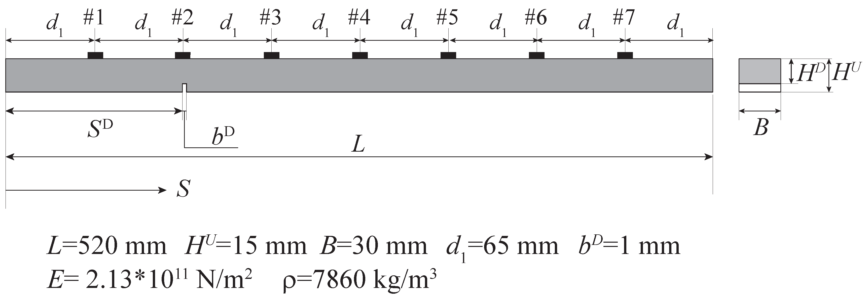
Figure 2.
Variation of modal displacements (a,b,c) and modal curvatures (d,e,f) in the four damage scenarios of location A, for the first (a,d), second (b,e) and third (c,f) mode.
Figure 2.
Variation of modal displacements (a,b,c) and modal curvatures (d,e,f) in the four damage scenarios of location A, for the first (a,d), second (b,e) and third (c,f) mode.
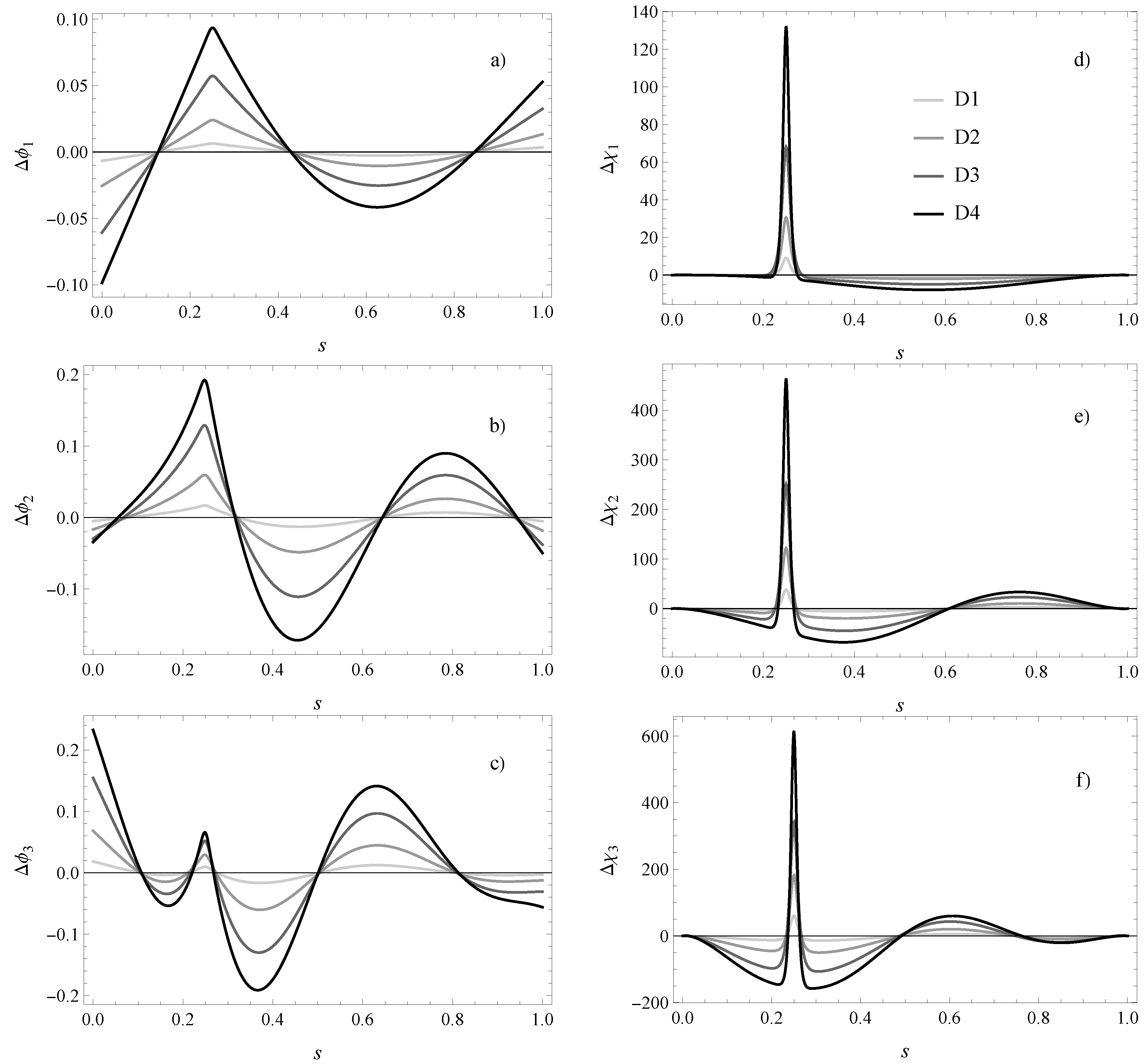
Figure 3.
Schematic representation of the experimental setup (a) and image of the beam in laboratory conditions (b).
Figure 3.
Schematic representation of the experimental setup (a) and image of the beam in laboratory conditions (b).
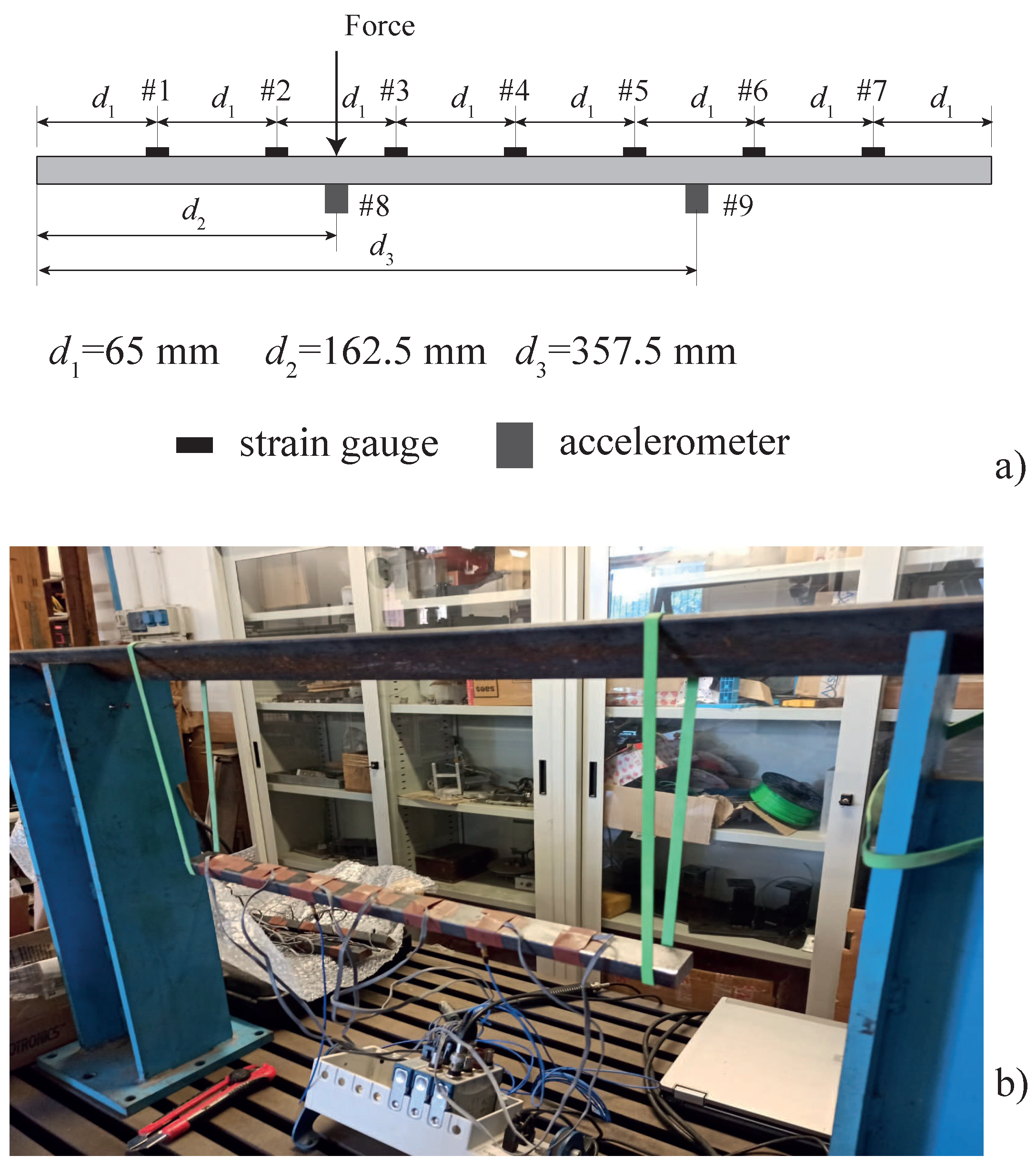
Figure 4.
Cases A: experimental (e) and numerical (n) modal curvatures (first (a), second (b) and third (c) mode) and their variations due to damage (first (d), second (e) and third (f) mode).
Figure 4.
Cases A: experimental (e) and numerical (n) modal curvatures (first (a), second (b) and third (c) mode) and their variations due to damage (first (d), second (e) and third (f) mode).

Figure 5.
Cases B: experimental (e) and numerical (n) modal curvatures (first (a), second (b) and third (c) mode) and their variations (first (d), second (e) and third (f) mode) due to damage.
Figure 5.
Cases B: experimental (e) and numerical (n) modal curvatures (first (a), second (b) and third (c) mode) and their variations (first (d), second (e) and third (f) mode) due to damage.
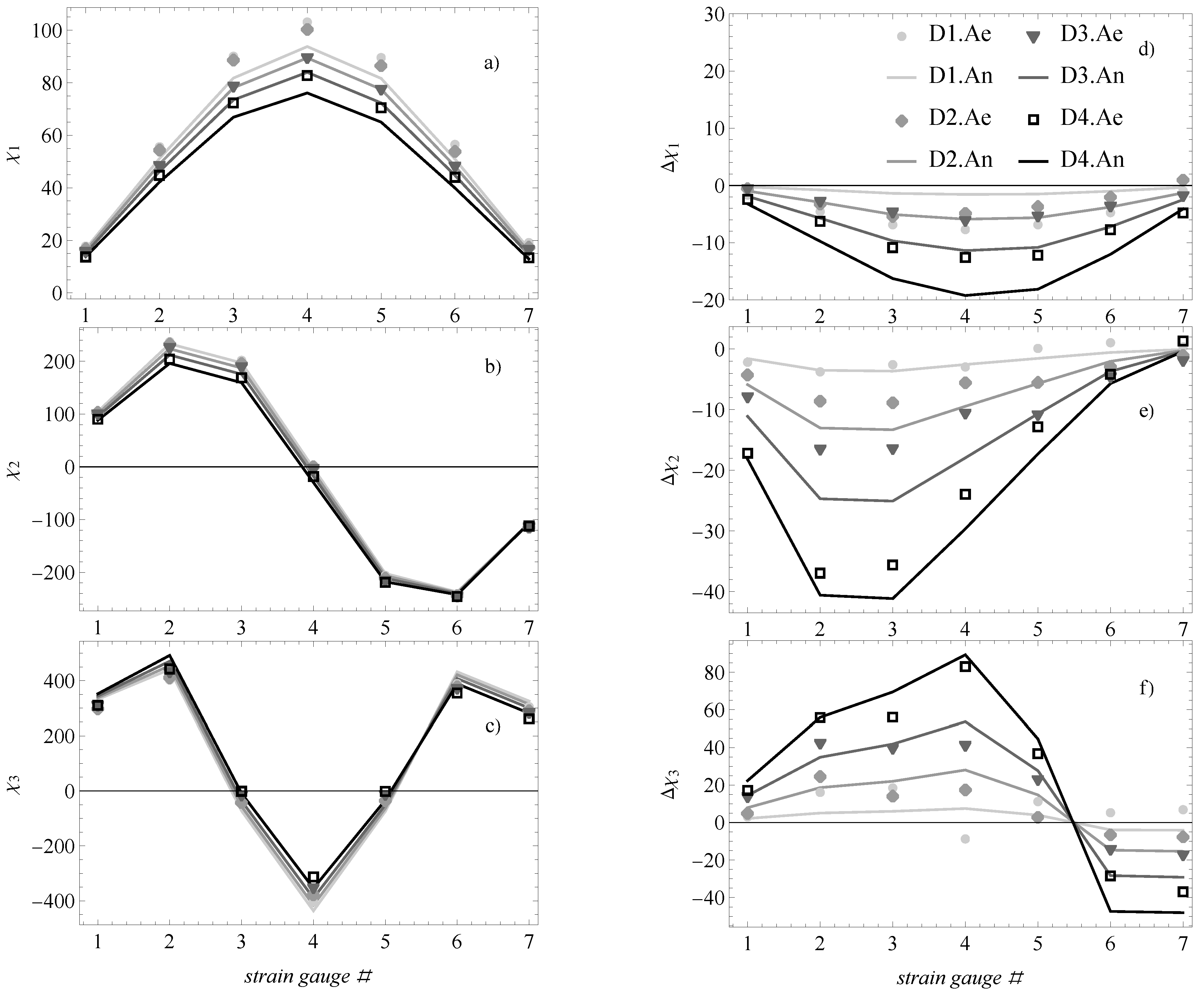
Figure 6.
Contour plots of the objective function including one (a i=1, b i=2, c i=3) and three numerical modal curvatures (i=1,2,3) (coordinates of the circle are and for D2.A).
Figure 6.
Contour plots of the objective function including one (a i=1, b i=2, c i=3) and three numerical modal curvatures (i=1,2,3) (coordinates of the circle are and for D2.A).
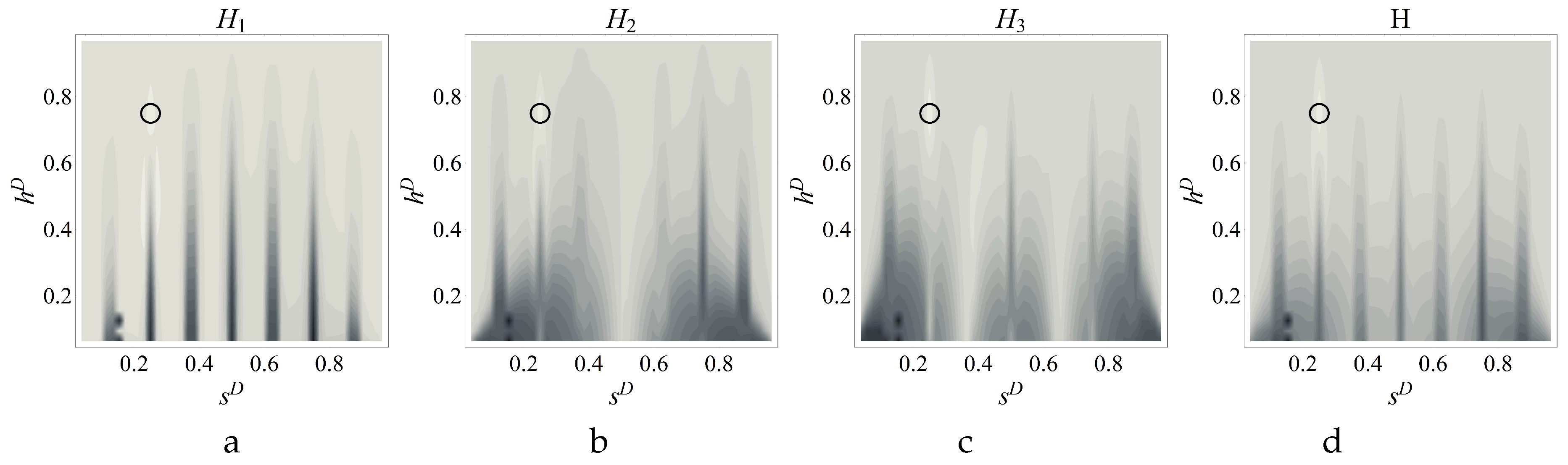
Figure 7.
Contour plots of the Bartlett beamformer including one (a i=1, b i=2, c i=3) and three numerical modal curvatures (i=1,2,3) (coordinates of the circle are and for D2.A).
Figure 7.
Contour plots of the Bartlett beamformer including one (a i=1, b i=2, c i=3) and three numerical modal curvatures (i=1,2,3) (coordinates of the circle are and for D2.A).
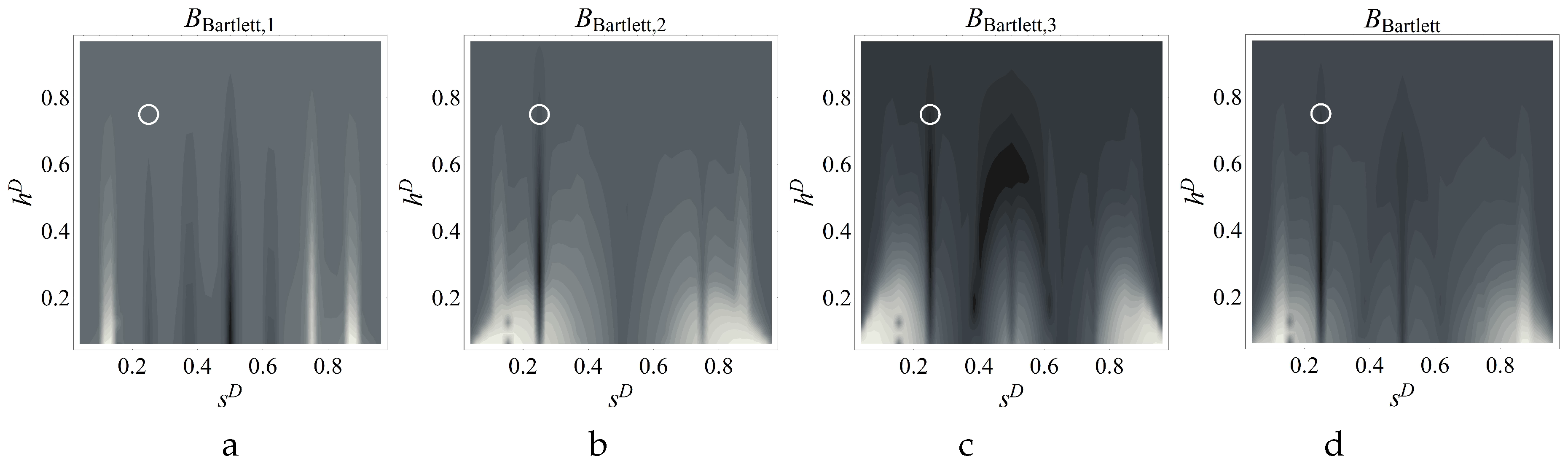
Figure 8.
Contour plots of the MVDR beamformer including one (a i=1, b i=2, c i=3) and three numerical modal curvatures (i=1,2,3) (coordinates of the circle are and for D2.A).
Figure 8.
Contour plots of the MVDR beamformer including one (a i=1, b i=2, c i=3) and three numerical modal curvatures (i=1,2,3) (coordinates of the circle are and for D2.A).
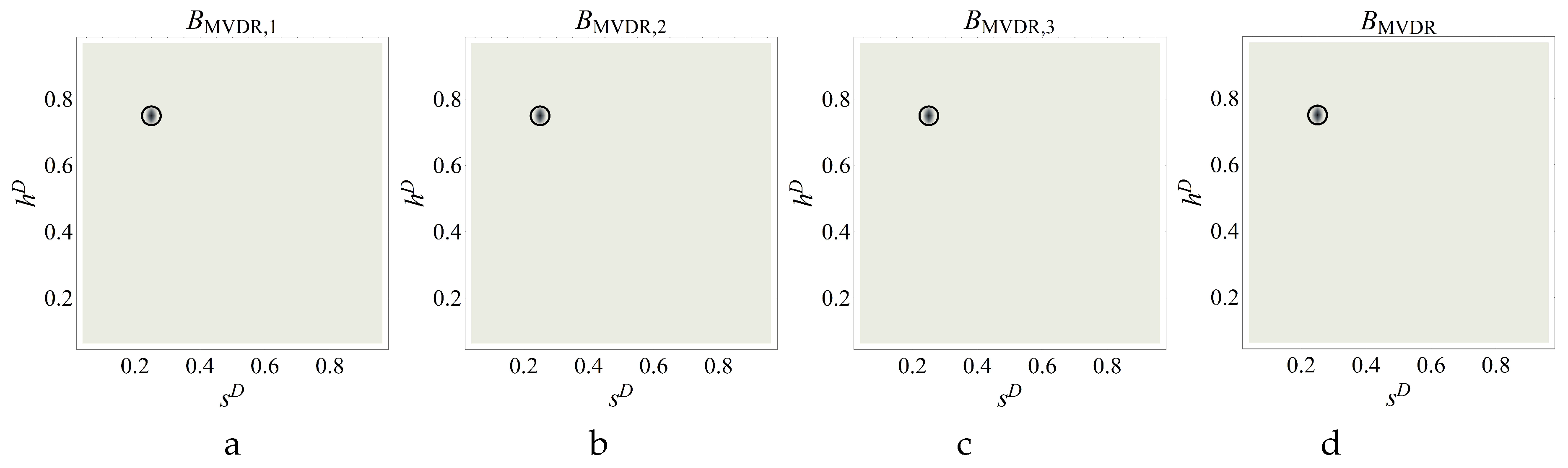
Figure 9.
Contour plots of the objective function including one (a i=1, b i=2, c i=3) and three numerical modal curvatures (i=1,2,3) (Circle: Correct damage parameters).
Figure 9.
Contour plots of the objective function including one (a i=1, b i=2, c i=3) and three numerical modal curvatures (i=1,2,3) (Circle: Correct damage parameters).
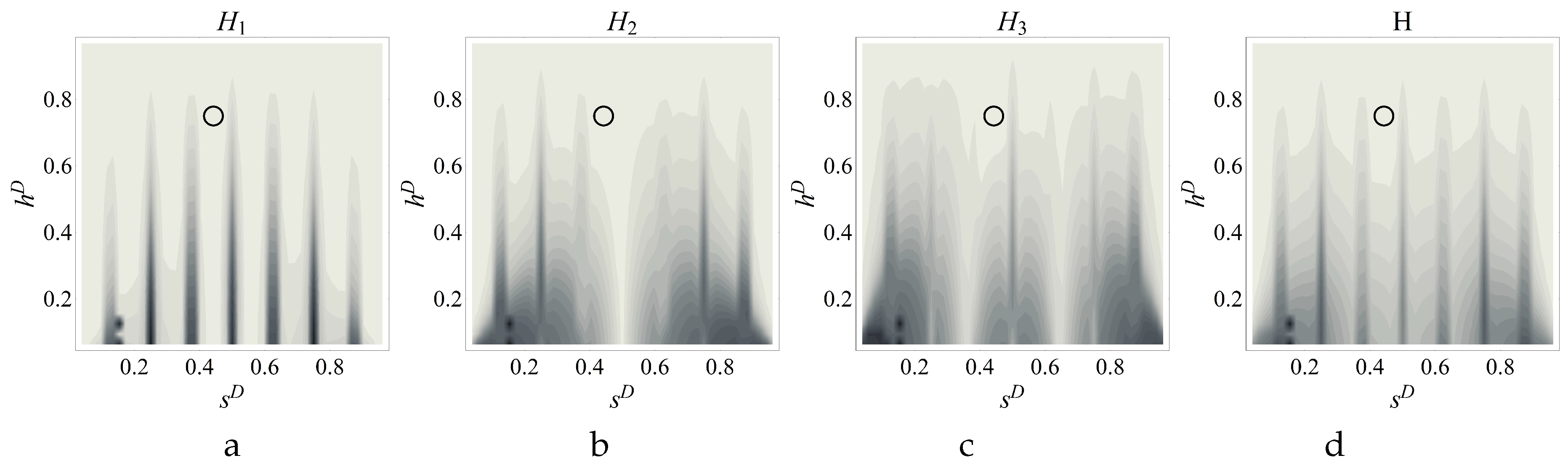
Figure 10.
Contour plots of the Bartlett beamformer including one (a i=1, b i=2, c i=3) and three numerical modal curvatures (i=1,2,3) (Circle: Correct damage parameters).
Figure 10.
Contour plots of the Bartlett beamformer including one (a i=1, b i=2, c i=3) and three numerical modal curvatures (i=1,2,3) (Circle: Correct damage parameters).
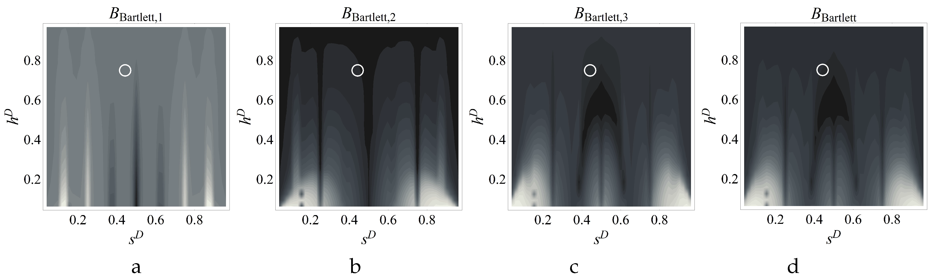
Figure 11.
Contour plots of the MVDR beamformer including one (a i=1, b i=2, c i=3) and three numerical modal curvatures (i=1,2,3) (Circle: Correct damage parameters).
Figure 11.
Contour plots of the MVDR beamformer including one (a i=1, b i=2, c i=3) and three numerical modal curvatures (i=1,2,3) (Circle: Correct damage parameters).
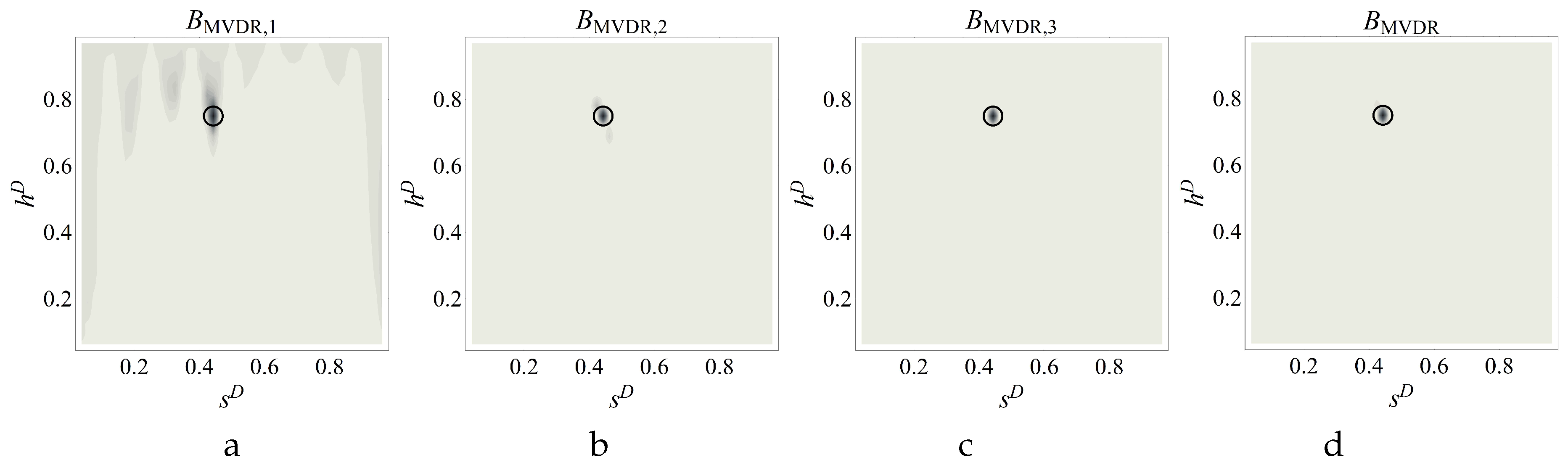
Figure 12.
Contour plots of the estimators for damage scenario D1.A (a) objective function, b) Bartlett, c) MVDR) (Circle: Correct damage parameters, Cross: identified parameters).
Figure 12.
Contour plots of the estimators for damage scenario D1.A (a) objective function, b) Bartlett, c) MVDR) (Circle: Correct damage parameters, Cross: identified parameters).
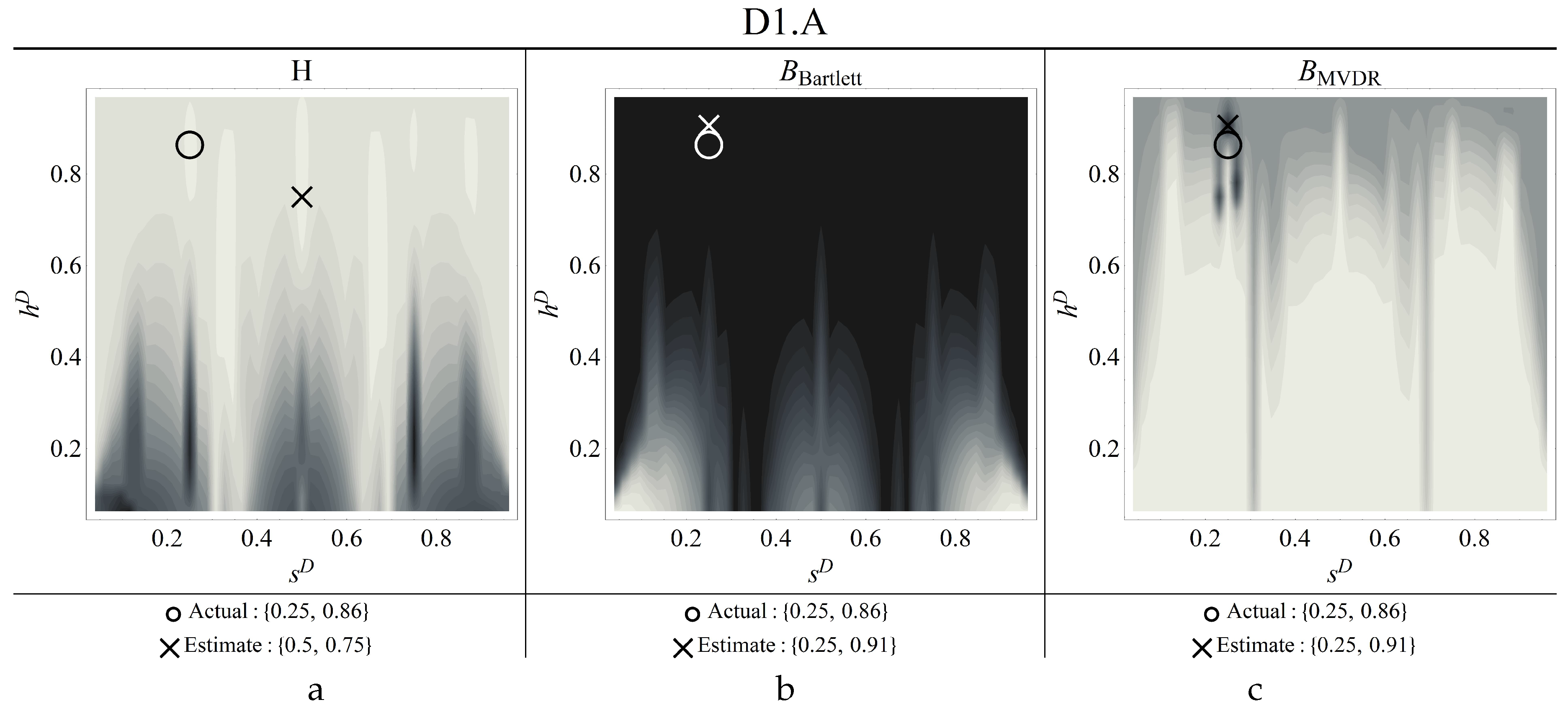
Figure 13.
Contour plots of the estimators for damage scenario D2.A (a) objective function, b) Bartlett, c) MVDR) (Circle: Correct damage parameters, Cross: identified parameters).
Figure 13.
Contour plots of the estimators for damage scenario D2.A (a) objective function, b) Bartlett, c) MVDR) (Circle: Correct damage parameters, Cross: identified parameters).
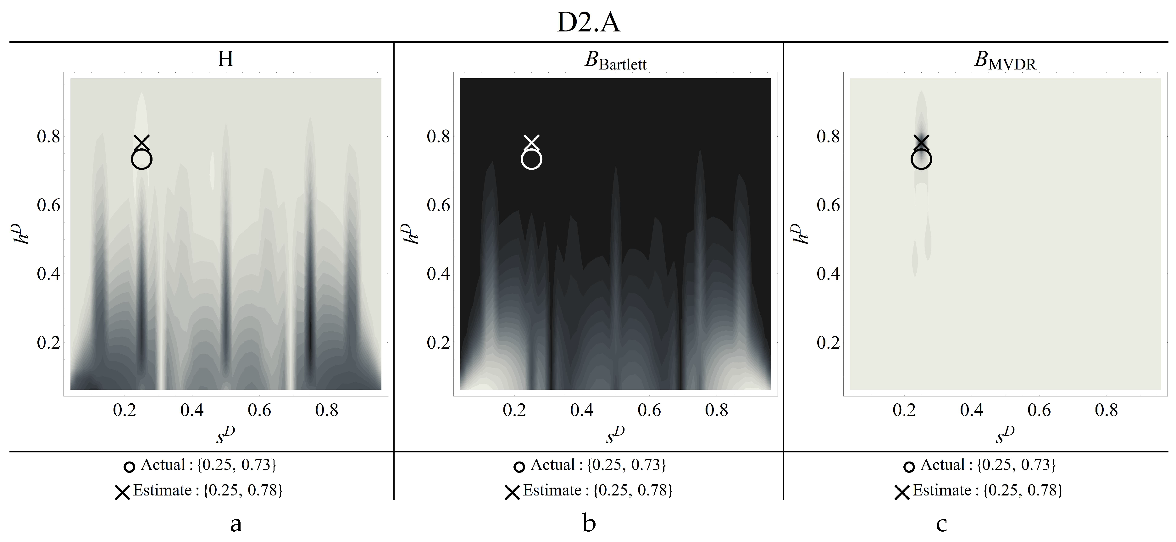
Figure 14.
Contour plots of the estimators for damage scenario D3.A (a) objective function, b) Bartlett, c) MVDR) (Circle: Correct damage parameters, Cross: identified parameters).
Figure 14.
Contour plots of the estimators for damage scenario D3.A (a) objective function, b) Bartlett, c) MVDR) (Circle: Correct damage parameters, Cross: identified parameters).
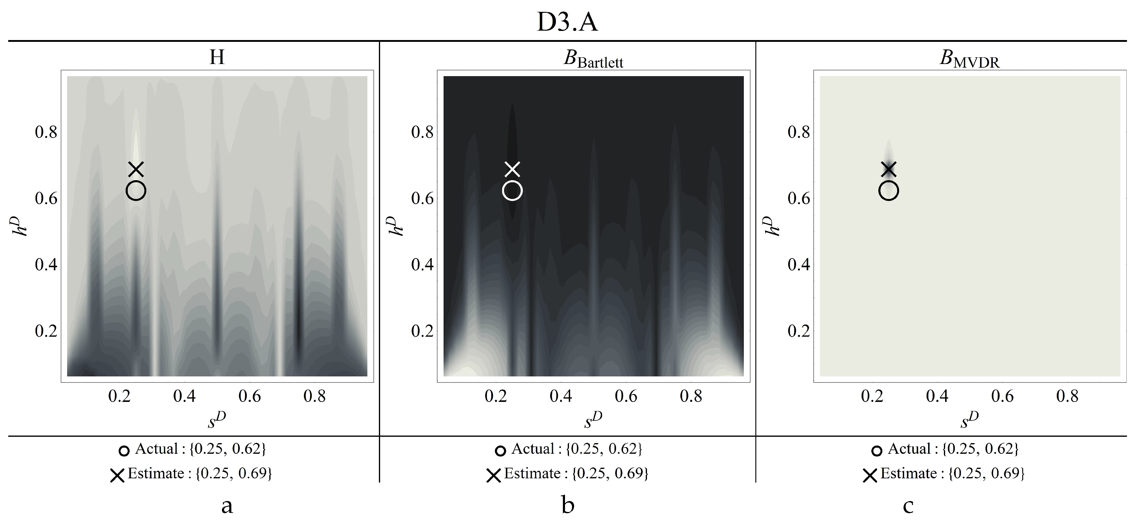
Figure 15.
Contour plots of the estimators for damage scenario D4.A (a) objective function, b) Bartlett, c) MVDR) (Circle: Correct damage parameters, Cross: identified parameters).
Figure 15.
Contour plots of the estimators for damage scenario D4.A (a) objective function, b) Bartlett, c) MVDR) (Circle: Correct damage parameters, Cross: identified parameters).
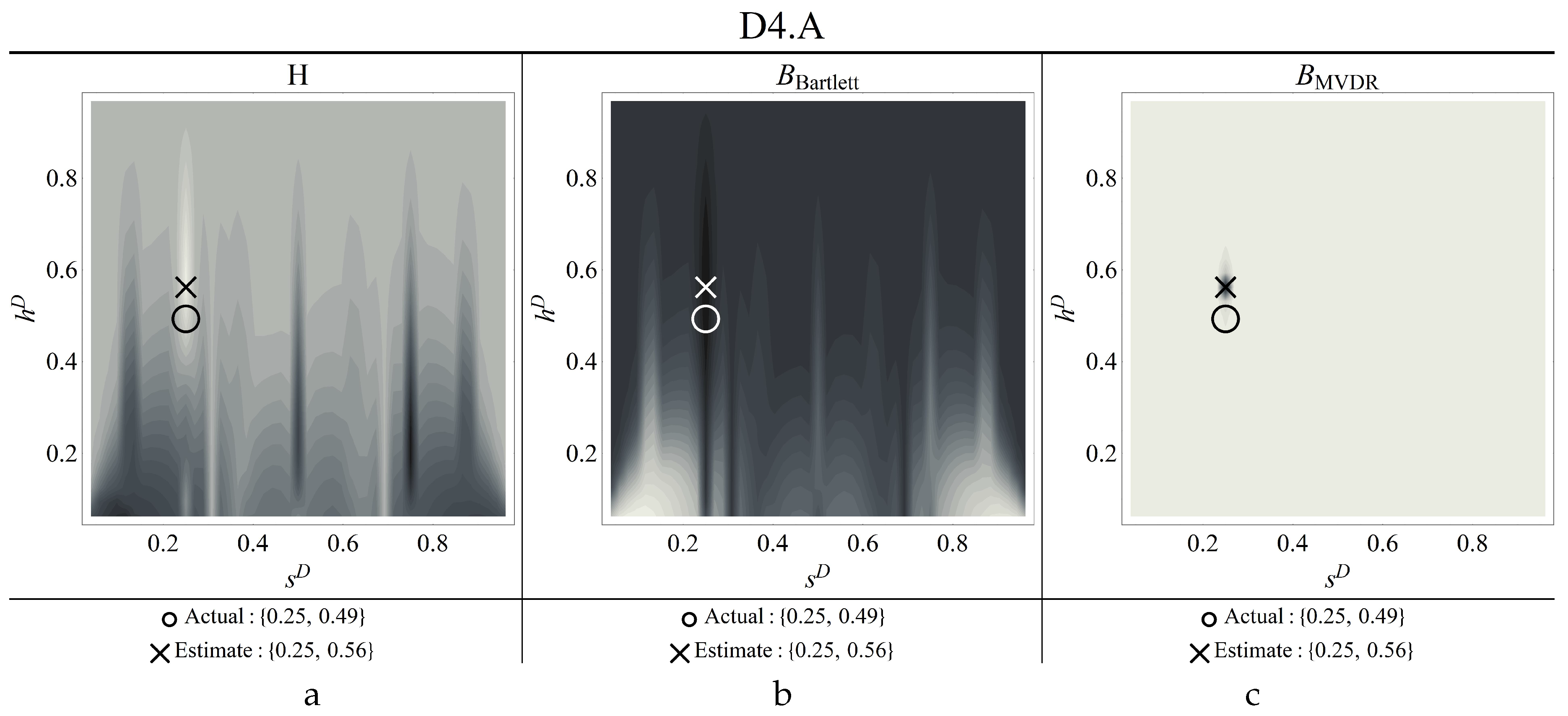
Figure 16.
Contour plots of the estimators for damage scenario D1.B (a) objective function, b) Bartlett, c) MVDR) (Thick circle: Correct damage parameters, Cross: identified parameters).
Figure 16.
Contour plots of the estimators for damage scenario D1.B (a) objective function, b) Bartlett, c) MVDR) (Thick circle: Correct damage parameters, Cross: identified parameters).
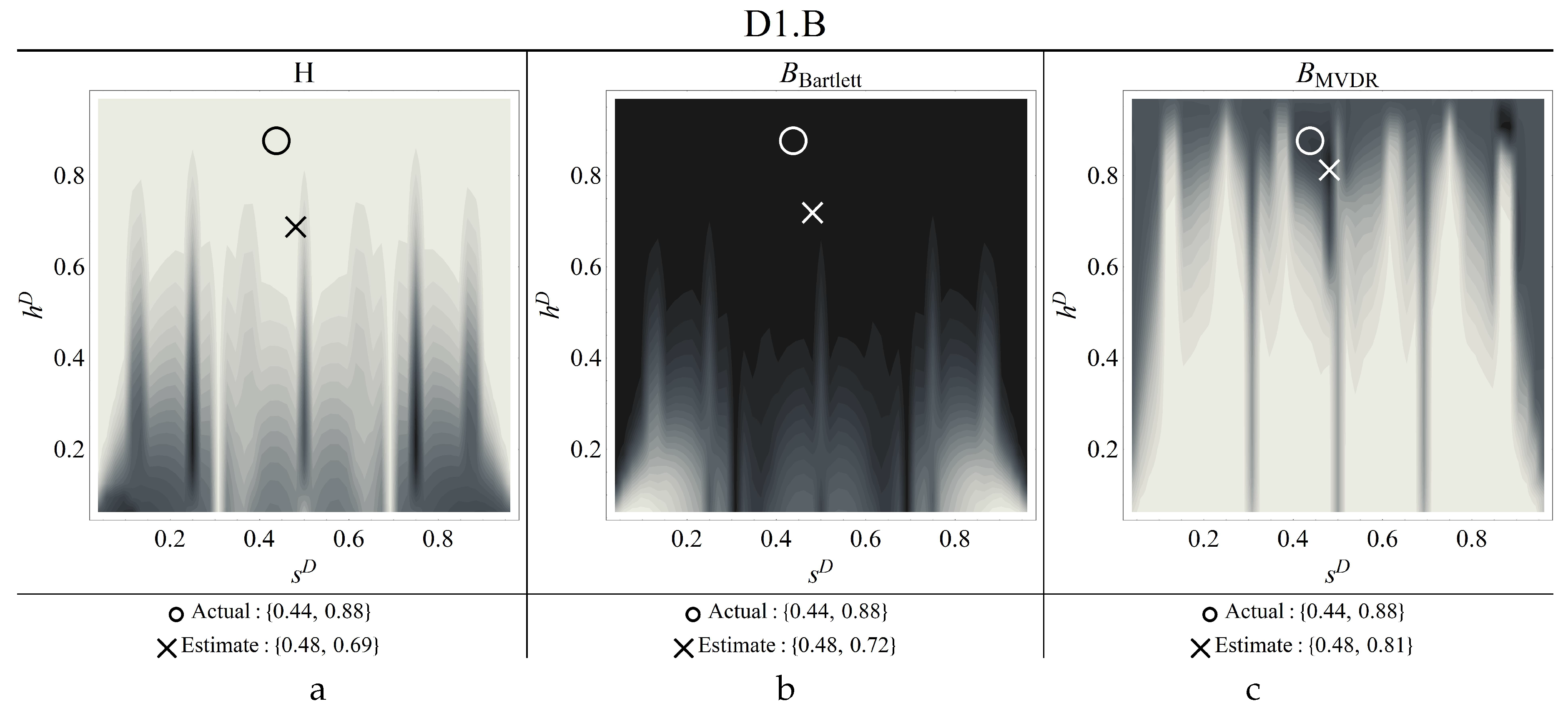
Figure 17.
Contour plots of the estimators for damage scenario D2.B (a) objective function, b) Bartlett, c) MVDR) (Thick circle: Correct damage parameters, Thin concentric circles: identified parameters).
Figure 17.
Contour plots of the estimators for damage scenario D2.B (a) objective function, b) Bartlett, c) MVDR) (Thick circle: Correct damage parameters, Thin concentric circles: identified parameters).
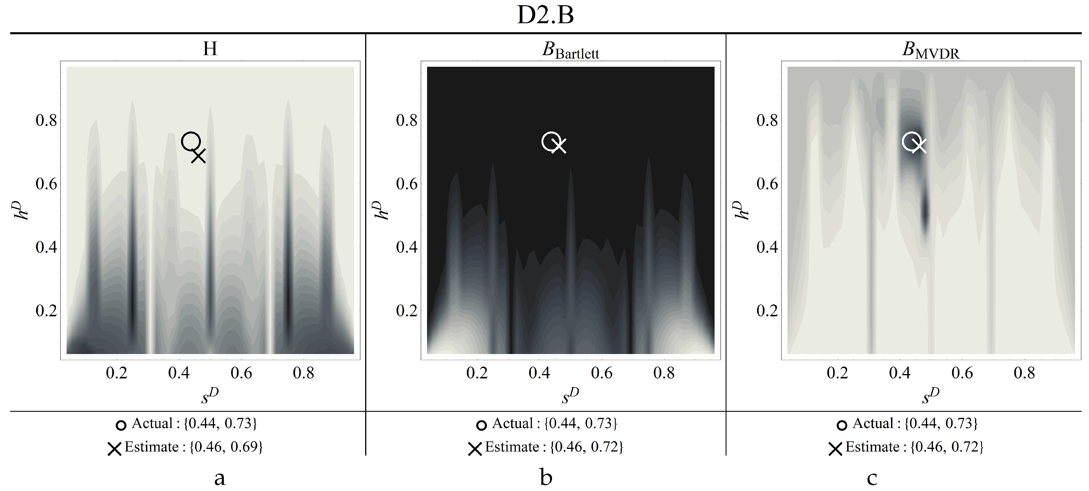
Figure 18.
Contour plots of the estimators for damage scenario D3.B (a) objective function, b) Bartlett, c) MVDR) (Thick circle: Correct damage parameters, Thin concentric circles: identified parameters).
Figure 18.
Contour plots of the estimators for damage scenario D3.B (a) objective function, b) Bartlett, c) MVDR) (Thick circle: Correct damage parameters, Thin concentric circles: identified parameters).
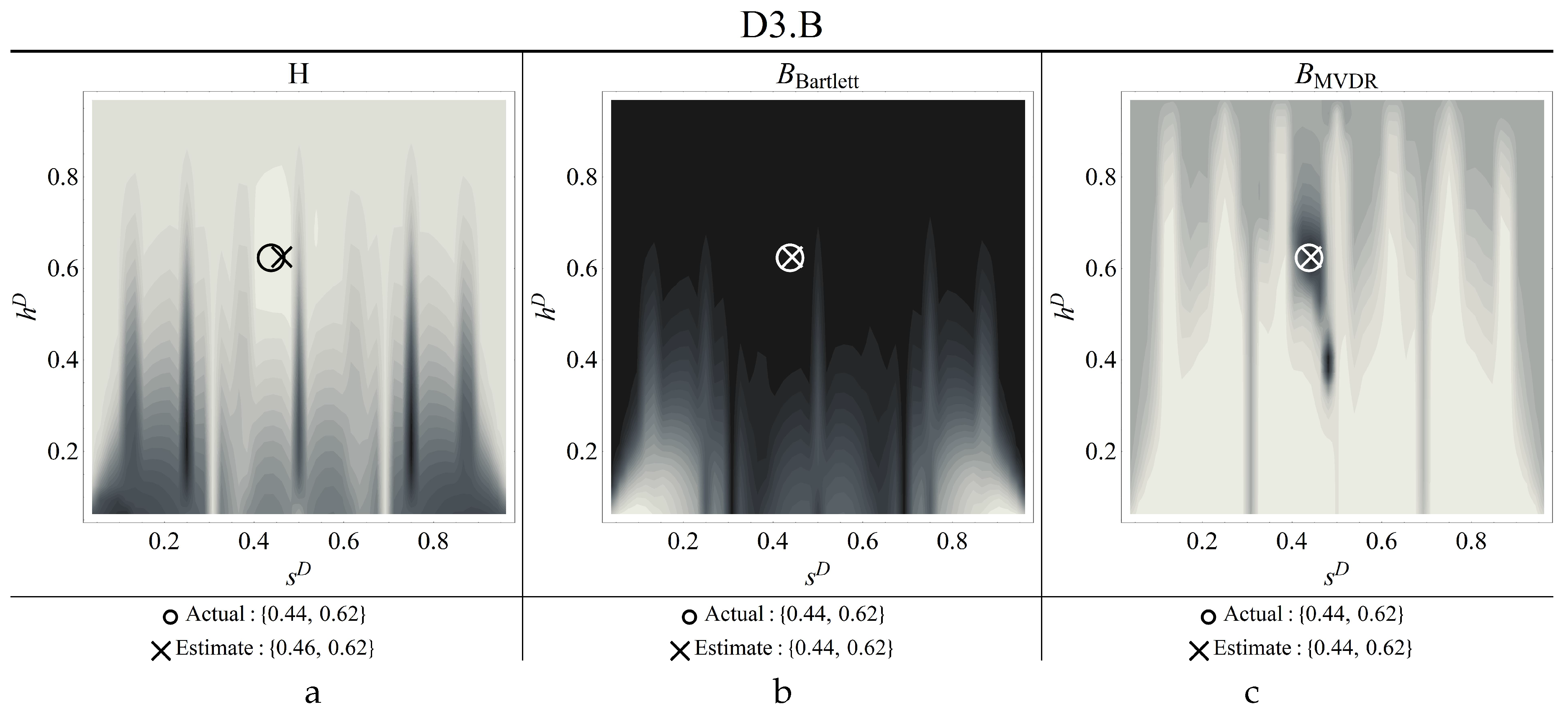
Figure 19.
Contour plots of the estimators for damage scenario D4.B (a) objective function, b) Bartlett, c) MVDR) (Circle: Correct damage parameters, Cross: identified parameters).
Figure 19.
Contour plots of the estimators for damage scenario D4.B (a) objective function, b) Bartlett, c) MVDR) (Circle: Correct damage parameters, Cross: identified parameters).
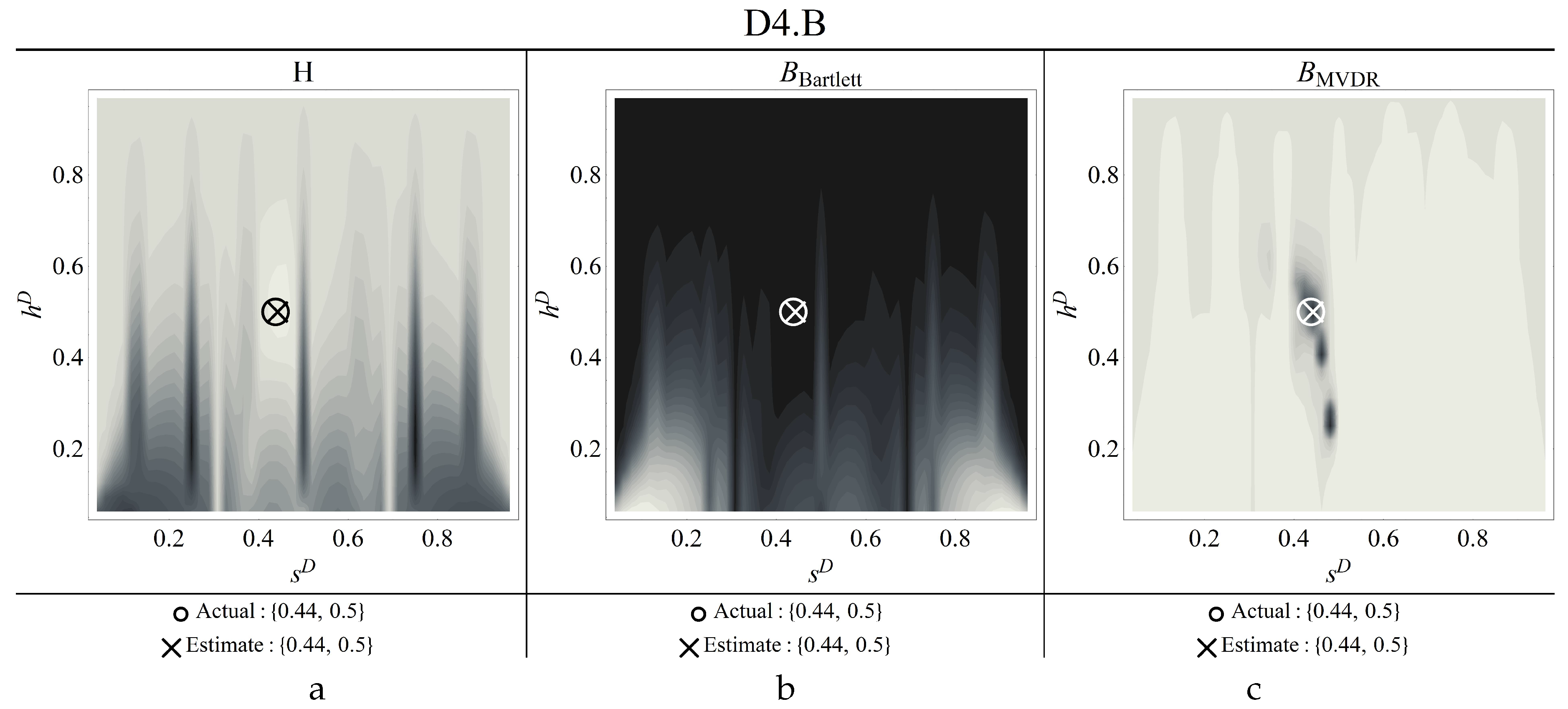

Table 1.
Labels of the damage scenarios with location (), nominal height of the damaged cross-section (), and percent stiffness reduction ().
Table 1.
Labels of the damage scenarios with location (), nominal height of the damaged cross-section (), and percent stiffness reduction ().
| D1.A | D2.A | D3.A | D4.A | D1.B | D2.B | D3.B | D4.B | |
|---|---|---|---|---|---|---|---|---|
| 0.25 | 0.25 | 0.25 | 0.25 | 0.4375 | 0.4375 | 0.4375 | 0.4375 | |
| 33.0 | 57.8 | 75.6 | 87.5 | 33.0 | 57.8 | 75.6 | 87.5 |
Table 2.
Numerical natural frequencies () [Hz] of the first three modes () and their percent variation () due to damage.
Table 2.
Numerical natural frequencies () [Hz] of the first three modes () and their percent variation () due to damage.
| U | D1.A | D2.A | D3.A | D4.A | ||
|---|---|---|---|---|---|---|
| 298.96 | 298.23 | 296.12 | 292.06 | 284.09 | ||
| 0.25 | 0.95 | 2.31 | 4.98 | |||
| 817.12 | 811.67 | 796.67 | 769.99 | 725.52 | ||
| 0.67 | 2.50 | 5.77 | 11.21 | |||
| 1582.02 | 1572.86 | 1549.21 | 1512.15 | 1546.32 | ||
| 0.58 | 2.07 | 4.23 | 7.39 | |||
| U | D1.B | D2.B | D3.B | D4.B | ||
| 298.96 | 295.28 | 290.78 | 279.95 | 261.29 | ||
| 1.23 | 2.73 | 6.36 | 12.60 | |||
| 817.12 | 810.97 | 809.69 | 800.44 | 785.54 | ||
| 0.75 | 0.91 | 2.04 | 3.87 | |||
| 1582.02 | 1570.62 | 1568.89 | 1552.45 | 1525.23 | ||
| 0.72 | 0.83 | 1.87 | 3.59 |
Table 3.
Damage scenarios with measured heights of the damaged cross-section ( [mm]), and percent stiffness reduction ().
Table 3.
Damage scenarios with measured heights of the damaged cross-section ( [mm]), and percent stiffness reduction ().
| D1.A | D2.A | D3.A | D4.A | D1.B | D2.B | D3.B | D4.B | |
|---|---|---|---|---|---|---|---|---|
| 13.3 | 11.3 | 9.6 | 7.6 | 13.2 | 11.0 | 9.4 | 7.5 | |
| 30.3 | 57.2 | 73.8 | 87.0 | 31.9 | 60.6 | 75.4 | 87.5 |
Table 4.
Geometrical and mechanical properties of the beams used in cases A and B.
| H [mm] | B [mm] | [mm] | E [GPa] | [kg/m] | |
|---|---|---|---|---|---|
| A | 15.40 | 30.12 | 130.0 | 206.5 | 7504.5 |
| B | 15.40 | 30.20 | 227.5 | 209.0 | 7656.8 |
Table 5.
Cases A: experimental () and numerical () natural frequencies [Hz] of the first three modes (), and their percent variation (,) due to damage.
Table 5.
Cases A: experimental () and numerical () natural frequencies [Hz] of the first three modes (), and their percent variation (,) due to damage.
| U | 298.8 | 813.52 | 1589.8 | ||||
| D1.A | 298.2 | 0.21 | 810.5 | 0.38 | 1584.6 | 0.32 | |
| D2.A | 296.8 | 0.68 | 797.8 | 1.98 | 1561.3 | 1.79 | |
| D3.A | 294.1 | 1.58 | 784.5 | 3.57 | 1540.3 | 3.11 | |
| D4.A | 288.7 | 3.40 | 753.2 | 7.41 | 1497.6 | 5.80 | |
| U | 298.8 | 814.5 | 1588.3 | ||||
| D1.A | 298.2 | 0.17 | 810.6 | 0.47 | 1581.8 | 0.41 | |
| D2.A | 296.5 | 0.75 | 798.1 | 2.00 | 1561.6 | 1.68 | |
| D3.A | 293.7 | 1.69 | 779.1 | 4.34 | 1533.5 | 3.45 | |
| D4.A | 288.0 | 3.61 | 744.3 | 8.62 | 1489.4 | 6.23 |
Table 6.
Cases B: experimental () and numerical () natural frequencies [Hz] of the first three modes (), and their percent variation (,) due to damage.
Table 6.
Cases B: experimental () and numerical () natural frequencies [Hz] of the first three modes (), and their percent variation (,) due to damage.
| U | 297.7 | 809.8 | 1584.5 | ||||
| D1.B | 295.5 | 0.73 | 808.3 | 0.19 | 1579.0 | 0.35 | |
| D2.B | 287.8 | 3.33 | 803.5 | 0.78 | 1564.1 | 1.29 | |
| D3.B | 282.1 | 5.23 | 799.0 | 1.34 | 1549.6 | 2.20 | |
| D4.B | 267.6 | 10.12 | 790.0 | 2.45 | 1521.5 | 3.97 | |
| U | 297.5 | 811.2 | 1582.6 | ||||
| D1.B | 295.1 | 0.83 | 808.9 | 0.28 | 1578.7 | 0.26 | |
| D2.B | 288.1 | 3.16 | 802.6 | 1.06 | 1567.5 | 0.96 | |
| D3.B | 279.1 | 6.19 | 794.9 | 2.01 | 1553.5 | 1.85 | |
| D4.B | 265.7 | 10.68 | 784.3 | 3.32 | 1534.2 | 3.06 |
Table 7.
% errors on the identified damage parameters for damage cases A.
| D1.A | D2.A | D3.A | D4.A | |||||
|---|---|---|---|---|---|---|---|---|
| H | 100 | -12.7 | 0.0 | 6.9 | 0.0 | 11.3 | 0.0 | 14.3 |
| Bartlett | 0.0 | 5.8 | 0.0 | 6.9 | 0.0 | 11.3 | 0.0 | 14.3 |
| MVDR | 0.0 | 5.8 | 0.0 | 6.9 | 0.0 | 11.3 | 0.0 | 14.3 |
Table 8.
% errors on the identified damage parameters for damage cases B.
| D1.B | D2.B | D3.B | D4.B | |||||
|---|---|---|---|---|---|---|---|---|
| H | 9.1 | -21.6 | 4.6 | -5.5 | 4.6 | 0.0 | 0.0 | 0.0 |
| Bartlett | 9.1 | -18.2 | 4.6 | -1.4 | 0.0 | 0.0 | 0.0 | 0.0 |
| MVDR | 9.1 | -8.0 | 4.6 | -1.4 | 0.0 | 0.0 | 0.0 | 0.0 |
Disclaimer/Publisher’s Note: The statements, opinions and data contained in all publications are solely those of the individual author(s) and contributor(s) and not of MDPI and/or the editor(s). MDPI and/or the editor(s) disclaim responsibility for any injury to people or property resulting from any ideas, methods, instructions or products referred to in the content. |
© 2023 by the authors. Licensee MDPI, Basel, Switzerland. This article is an open access article distributed under the terms and conditions of the Creative Commons Attribution (CC BY) license (https://creativecommons.org/licenses/by/4.0/).
Copyright: This open access article is published under a Creative Commons CC BY 4.0 license, which permit the free download, distribution, and reuse, provided that the author and preprint are cited in any reuse.


