Neither Zero-Catch Data nor Model Structure. Noisy Labels Are the Key Hindrance of Improving Fisheries Forecasting Performance

1. Introduction

For the fisheries forecasting task of by-catches, the dataset is filled with a large number of samples with zeros of CPUE, which we refer to as zero-catch data, and refer to the phenomenon of a large number of zeros in the dataset as the zero-catch problem. The existence of zero-catch data involves many uncertainties, such as the failure or destruction of fishing vessels or gear, errors in the data recording process, or the fact that the area of fishing operation is indeed unsuitable for fisheries survival[1]. It’s too complex for researchers to determine whether the existence of zero-catch data in the grids is due to the chance of the fishing process or the inevitability of the expression of marine environmental factors. Since zero-catch data can distract the machine learning model training and forecasting tasks performed on dataset(especially by-catches dataset), the zero-catch problem cannot be avoided if we want to improve the performance of the model for fisheries forecasting.

Previous works have tended to treat zero values uniformly[2,3,4,5,6,7,8,9]. One of the clearest methods is to directly discard all zero-catch data, which obviously loses some correctly-labeled samples. In order to ensure the completeness of the dataset as much as possible, a simpler method is to improve the data granularity of the spatio-temporal factor[2], i.e., to change the temporal resolution of the CPUE from days to months, or to decrease the spatial resolution of the CPUE from $0.5^{\circ }\times 0.5^{\circ }$ to $1^{\circ }\times 1^{\circ }$. However, the result of the fishery prediction obtained by this treatment is rough, and its usefulness for the fishing of fishery resources in reality is relatively limited. In order to eliminate the negative impact of zero-catch data and obtain more accurate results, a common method is to add a constant to all the values with CPUE of 0. However, the process of determining the constant[3,4] is relatively arbitrary, and the set constant is not necessarily applicable to other fisheries forecasting tasks, because there are differences in the probability distributions[5] of each fishery dataset, and it is difficult to accurately characterize the probability distribution model of a fishery dataset to accurately describe it. In order to avoid the interference from zero-catch samples in the training process of fishery forecasting models, some researchers have adopted the delta method[1,6,7] to fit zero-catch samples and non-zero samples using two relatively independent statistical models, but both non-zero samples and zero-catch samples are derived from fishery datasets in the same marine environment and spatio-temporal scales, and it is therefore difficult to find two relatively independent statistical models that fit these two types of data separately.

All of the above work are the uniform treatments to zero-catch data, but obviously not all zero-catch data are anomalous, in order to further research those anomalous zero-catch data, researchers use the zero-inflated[8,9] model to analyze the causes of the zero-catch data. However, it is only a qualitative analysis of the zero-catch data in terms of the number of zero-catch data, which cannot be analyzed for each specific sample, and moreover, real-world fishery datasets have a probability distributions are often irregular and a practical model that perfectly fits the test set cannot be easily obtained.

To the best of our knowledge, there is no effective method to detect whether non-zero samples in the fishery dataset are anomalous or not. In order to correct all anomalous samples in a fishery dataset and to identify the cause of each anomalous sample, we proposes a confident learning[10] based method for detecting anomalous fishery samples, which analyzes the zero-catch samples and non-zero samples (the anomalous ones) by treating them uniformly as noises in the dataset. Quantitatively, it reveals the heterogeneity that exists among zero-catch samples as well as among non-zero samples, i.e., it is possible for the samples to be observed with labels that are different from the ones that should have been expressed. In addition, the methodology presented in this paper was experimented on three tuna datasets from 2016 to 2019 in tropical waters of the Atlantic ocean[11]. A large number of anomalous samples were detected on both the by-catch dataset, which has a high number of zero-catch samples, as well as the main catch dataset, which has a relatively sparse number of zero-catch samples, and after repairing those anomalous samples, the performance of the fishery forecasting model(Random Forests, Support Vector Machine and XGBoost),which are classical in the field of machine learning, gained a more substantial improvement than that feedback on the original dataset before.

2. Materials and Methods

2.1. Dataset

The datasets mainly, which were collected from three species of tuna, include the original fishery data and the marine environment factors. The raw fishery data were collected from the fishing logbooks in the tropical waters of the Atlantic Ocean from 2016 to 2019, including vessel name, operation date(day/month/year), operation site (latitude and longitude of the start position of each deployment, and fishery information (species/daily catch/hook numbers), and the fishing area was limited in ${14}^{\circ }{20}^{\prime }S$-${15}^{\circ }{20}^{\prime }N,{47}^{\circ }{38}^{\prime }W$–$2^{\circ }{30}^{\prime }E$. 29 environmental factors include chlorophyll-a concentration (chl-a); Wind Speed on the sea surface (WS), Eddy Kinetic Energy (EKE), Mixed Layer Depth (MLD), the vertical temperature and dissolved oxygen concentration of 0, 50, 100, 200, 250, 300, 350, 400, 450, and 500m below the sea surface(respectively abbreviated as T0, T50, T100, T200, T250, T300, T350, T400, T450, T500, D0, D50, D100, D200, D250, D300, D350, D400, D450, and D500); and the vertical salinity of 100, 200, 400 and 500m below the sea surface(abbreviated as S100, S200, S400, and S500). The wind speed data were derived from the database in the National Oceanic and Atmospheric Administration (https://oceanwatch.pifsc.noaa.gov/). Other data were all downloaded from the Copernicus Marine Environmental Monitoring Service center (http://marine.copernicus.eu). The temporal resolution in all the datasets is modified in days, and the spatial resolution is also modified in $0.5^{\circ }\times 0.5^{\circ }$ uniformly. The rough CPUE distribution of the three tuna species is shown in Table 1.

Table 1. The first quantile (Q1) and the second quantile (Q2) of three tuna sepecies datasets in the grids of $0.5^{\circ }\times 0.5^{\circ }$

Dataset	Q11	Q21
Yellowfin tuna	0	0.435
Albacore tuna	0	0.833
Bigeye tuna	5	10.4

¹ The first quantile of CPUE(individuals per 1000 hooks). ² The second quantile of CPUE(individuals per 1000 hooks).

Table 1. The first quantile (Q1) and the second quantile (Q2) of three tuna sepecies datasets in the grids of $0.5^{\circ }\times 0.5^{\circ }$

Dataset	Q11	Q21
Yellowfin tuna	0	0.435
Albacore tuna	0	0.833
Bigeye tuna	5	10.4

¹ The first quantile of CPUE(individuals per 1000 hooks). ² The second quantile of CPUE(individuals per 1000 hooks).

2.2. Data preprocess

The formula for calculating CPUE in each grid is as follows[12]:

$$CPU{E}_{kmnij}=\frac{F_{kmnij}}{H_{kmnij}}\times 1000$$

(1)

where $CPU{E}_{kmnij},F_{kmnij},and{H}_{kmnij}$ are the CPUE, total individual catch of tuna, and the number of hooks in k year, m month, n day, grid longitude i, grid latitude j, respectively. Bi-variate correlation analysis of CPUE with all spatial, temporal and marine environmental factors in a grid with a temporal resolution of days and a spatial resolution of $0.5^{\circ }\times 0.5^{\circ }$ was carried out by using the statistical software SPSS 23.0 to compute the Pearson correlation coefficients(P) and test for significance (assuming that the level of significance is 0.05, i.e., P is less than 0.05), and the correlation coefficients, R, took values in the range of correlation coefficient R is [-1, 1], and the larger the absolute value of R, the stronger the correlation between the two variables. Environmental variables with P greater than 0.05 were deleted for subsequent multicollinearity analysis.

The purpose of multicollinearity analysis of independent variables is to prevent the covariance relationship existing between variables from interfering with the forecasting process of the model, and the performance of which is rather reduced when there are more environmental factors. In order to exclude the potential high correlation between the marine environmental factors and the spatio-temporal variables, whether there is multicollinearity between the variables was judged according to Variance Inflation Factor[13] (VIF), and the marine environmental factors with VIF less than 10 were retained, and the variables with multicollinearity were deleted, which was calculated as follows:

$$VIF=\frac{1}{1-R_i}$$

(2)

where $R_i$ is the correlation coefficient of the ith variable when regressed on all other variables. The diagnosis of multicollinearity ends when all variables with VIF greater than 10 are filtered out. Since the scale and order of magnitude of the fishery production data and the marine environmental factors are not uniform, the role of variables in the data analysis would be affected by the size of the value itself if the raw data are used directly for analysis. In order to ensure the reliability of the experimental data, it is necessary to standardize the raw data. We used the data normalization method as shown below to map the value of each variable to the range of [0,1], and for each variable, the formula is:

$$x^{*}=\frac{x-x_{min}}{x_{max}-x_{min}}$$

(3)

where $x^{*}$ denotes the value of the variable after normalization, $x_{max}$ denotes the maximum value of the variable in the dataset, $x_{min}$ denotes the minimum value of the variable in the dataset, and x denotes the original value of the variable in the dataset.

2.3. Proposed method

How to solve the interference of noisy samples for model training while maximizing the value of the original data is an important topic in the direction of "learning with noisy labels[14](LWNL)" in the field of supervised learning. One feasible approach is to measure the differences between the noisy sample and the normal sample. Confident Learning grasps the whereabouts of the noise samples in the dataset by estimating the joint distribution between the noise samples and the normal samples and then outlining the demarcation between them. It does not work on model performance like other traditional LWNL methods, but takes an alternative approach, working from the sample itself, so it is a data-centered noise-containing learning method.

Firstly, the fishery dataset which is ready to be probed for noisy samples is cross-validated by any model which has the ability to classif the input samples (e.g., Random Forests, Support Vector Machine, XGBoost, Logistic Stochastic regression, etc.), and obtains the probability vector ${\widehat{\mathit{P}}}_k$ about each sample being classified in the every classes:

$${\widehat{\mathit{P}}}_k:=\left\{\left({\mathit{x}}_k,\tilde{y}\right)\in \left({\mathbb{R}}^d,{\mathbb{Z}}_{\ge 0}^{\left[m\right]}\right):\widehat{p}\left(\tilde{y}=i;{\mathit{x}}_k,\theta \right),i\in \left[m\right]\right\}$$

(4)

where $\left({\mathit{x}}_k,\tilde{y}\right)$ denotes the kth sample in the fishery dataset, and since a sample contains multiple marine environmental factors, the ${\mathit{x}}_k$ is bolded to indicate a feature vector. Since the confident learning model is discussed in terms of noisy samples only, $\tilde{y}$ denotes the noise label and therefore normal samples are not included in the analysis. In addition, $\left({\mathbb{R}}^d,{\mathbb{Z}}_{\ge 0}^{\left[m\right]}\right)$ denotes that the total number of marine environmental factors about the sample is d. The attribute space of the samples is a set of natural numbers and there are a total of m mutually exclusive class. Under the dichotomous condition, m equals to 2. $\widehat{p}\left(\tilde{y}=i;{\mathit{x}}_k,\theta \right)$ denotes the probability that the kth sample within the fishery dataset is misclassified as class i, and the probability matrix $\widehat{\mathit{P}}$ of the fishery dataset can be obtained by obtaining the probabilities vector${\widehat{\mathit{P}}}_k$ of misclassification from all the samples. It should be noted that the performance of the model will affect the the results of probing noisy samples, so it is better to choose a model that is robust[15] to noisy data so that the anomalous samples can be detected as many as possible. Through the probability matrix, we can find the confidence level t for each classification case. In fact, the confidence level is the core of "confidence" in confident learning. The confidence level is calculated as follows:

$$t_j=\frac{1}{\left|{\mathit{X}}_{\tilde{y}=j}\right|}\sum _{x\in {\mathit{X}}_{\tilde{y}=j}}\widehat{p}(\tilde{y}=j;\mathit{x},\mathit{\theta }),j\in \left[m\right]$$

(5)

where $t_j$ denotes the confidence level that a sample is classified as j . It is used to portray how difficult it is for the sample to be classified as class j . Note that the reason why the right side of the equation is divided by the total number of samples classified as j is to address the class-imbalance problem, as avoiding biased classification results due to the imbalance[16] in the weight of one class of samples among all samples. Dividing by the number of samples effectively solves the problem of class imbalance; If the number of samples classified as j is high, the confidence level of being classified as j is low; Conversely, if the number of samples classified as j is low, the threshold for confidence as j becomes high. Using the confidence level, we can obtain the class which each sample is actually most likely to be classified through the classification matrix ${\widehat{\mathit{X}}}_{\tilde{y}=i,y^{*}=j}$ as shown below:

$${\widehat{\mathit{X}}}_{\tilde{y}=i,y^{*}=j}:=\left\{x\in {\mathit{X}}_{\tilde{y}=i}:\widehat{p}(\tilde{y}=j;\mathit{x},\mathit{\theta }),j=\underset{l\in \left[m\right]:\widehat{p}(\tilde{y}=l;\mathit{x},\mathit{\theta })\ge t_l}{argmax}\widehat{p}(\tilde{y}=l;\mathit{x},\mathit{\theta })\right\}$$

(6)

where $y^{*}$ denotes the true label and then ${\widehat{\mathit{X}}}_{\tilde{y}=i,y^{*}=j}$ denotes the subset of samples where the noise sample is labeled i, but the label should actually be j. Samples that are not on the diagonal of this matrix are determined to be noise, i.e., anomalous samples. In the case of binary classification, we can repair those anomalous samples by reversing its labels.

3. Experiments

3.1. Preparation for evaluation

In order to eliminate the negative impact of the class imbalance problem as much as possible, we use Accuracy, Precision, Recall, F1-score, Receiver Operating Characteristic (ROC) and Area under Curve (AUC) to comprehensively evaluate the effectiveness of proposed method. Since the fishery forecasting problem in this paper can be statute to the problem of binary classification, we can record the samples labeled as "1" as positive cases P, and the samples labeled as "0" as negative cases N, then:

Accuracy indicates the proportion of samples whose prediction results are consistent with the actual labels of the samples, the accuracy reflects the differentiation ability of the model for the whole of the dataset, the higher the accuracy, the preciser the result of classification in the dataset, the formula is as follows:

$$Acc=\frac{100\%\times (TP+TN)}{TP+TN+FP+FN}$$

(7)

Where TP(True Positive) denotes the number of samples with positive actual labels and positive predictions; FN(False Negative) denotes the number of samples with positive actual labels and negative predictions; FP(False Positive) denotes the number of samples with negative actual labels and positive predictions; and TN(True Negative) denotes the number of samples with negative actual labels and negative predictions, and those abbreviations mentioned above are also used in the evaluation formulas below:

$$\mathcal{P}=\frac{TP}{TP+FP}$$

(8)

$$\mathcal{R}=\frac{TP}{TP+FP}$$

(9)

$$F_1=\frac{100\%\times \left(2\mathcal{P}\mathcal{R}\right)}{\mathcal{P}+\mathcal{R}}$$

(10)

As mentioned above, $\mathcal{P}$(Precision) indicates the proportion of positively labeled samples in the predicted positive samples. The higher the precision, the stronger the forecasting performance to identify negative samples. $\mathcal{R}$(Recall) indicates the proportion of samples predicted to be positive that are actually labeled as positive to the actual positive samples, the recall reflects the ability of the classifier to identify positive samples in the dataset, the higher the recall, then the stronger the forecasting performance to identify positive samples.$F_1$(F1 score) is used to assess the stability of the model classification performance.It denotes the reconciliation average of the model Precision and Recall, the value domain is [0, 1], the higher the F1 score, the better the comprehensive performance of the forecasting task.

The ROC curve is obtained by plotting the true rate TP and the false positive rate FP as the vertical and horizontal coordinates, respectively, and the AUC value is the area under the ROC and the horizontal coordinate with the value domain [0, 1].

The confusion matrix is a matrix which represents the forecasting results. In this paper, we use heat map to visualize the result of the binary classification in the datasets of the three tuna species. The numbers of TP, TN, FP, and FN obtained for each dataset are used to derive the confusion matrix of each species.

3.2. Environments

The operating system used for model training is Windows 10, the CPU model is Intel Core i7-10510U-2.30GHz, the GPU model is NVIDIA GeForce-MX250, the main memory size is 8G, the mass memory size is 2TB, the programming language is Python 3.7, and the development framework is scikit-learn 1.1.2.

3.3. Results

3.3.1. Anomalous samples analysis

In general, the stronger the predictive performance of the model, the more accurate the estimation of the true labels of the observed sample, i.e., the more accurate the judgment of the noisy samples in the dataset. However, the study of model performance is obviously not the focus of this paper, so we choose the classical random forests[17](other models are also optional) model to estimate the joint distribution of observed and true labels, and probe the proportion and nature of noise in the tuna datasets.

Table 2. Quantitative relationship between zeros and noisy samples in three datasets

Dataset1	Total number of zeros	Total number of noisy samples	Noisy samples in Zeros	Zeros in Noisy samples
Yellowfin tuna	5712	2812	53.77%	26.47%
Albacore tuna	4652	2206	43.20%	20.49%
Bigeye tuna	569	1608	6.15%	2.17%

¹ The total number of samples in each dataset is 11252.

Table 2. Quantitative relationship between zeros and noisy samples in three datasets

Dataset1	Total number of zeros	Total number of noisy samples	Noisy samples in Zeros	Zeros in Noisy samples
Yellowfin tuna	5712	2812	53.77%	26.47%
Albacore tuna	4652	2206	43.20%	20.49%
Bigeye tuna	569	1608	6.15%	2.17%

¹ The total number of samples in each dataset is 11252.

Figure 1. Confusion matrix for each tuna dataset

Figure 1. Confusion matrix for each tuna dataset

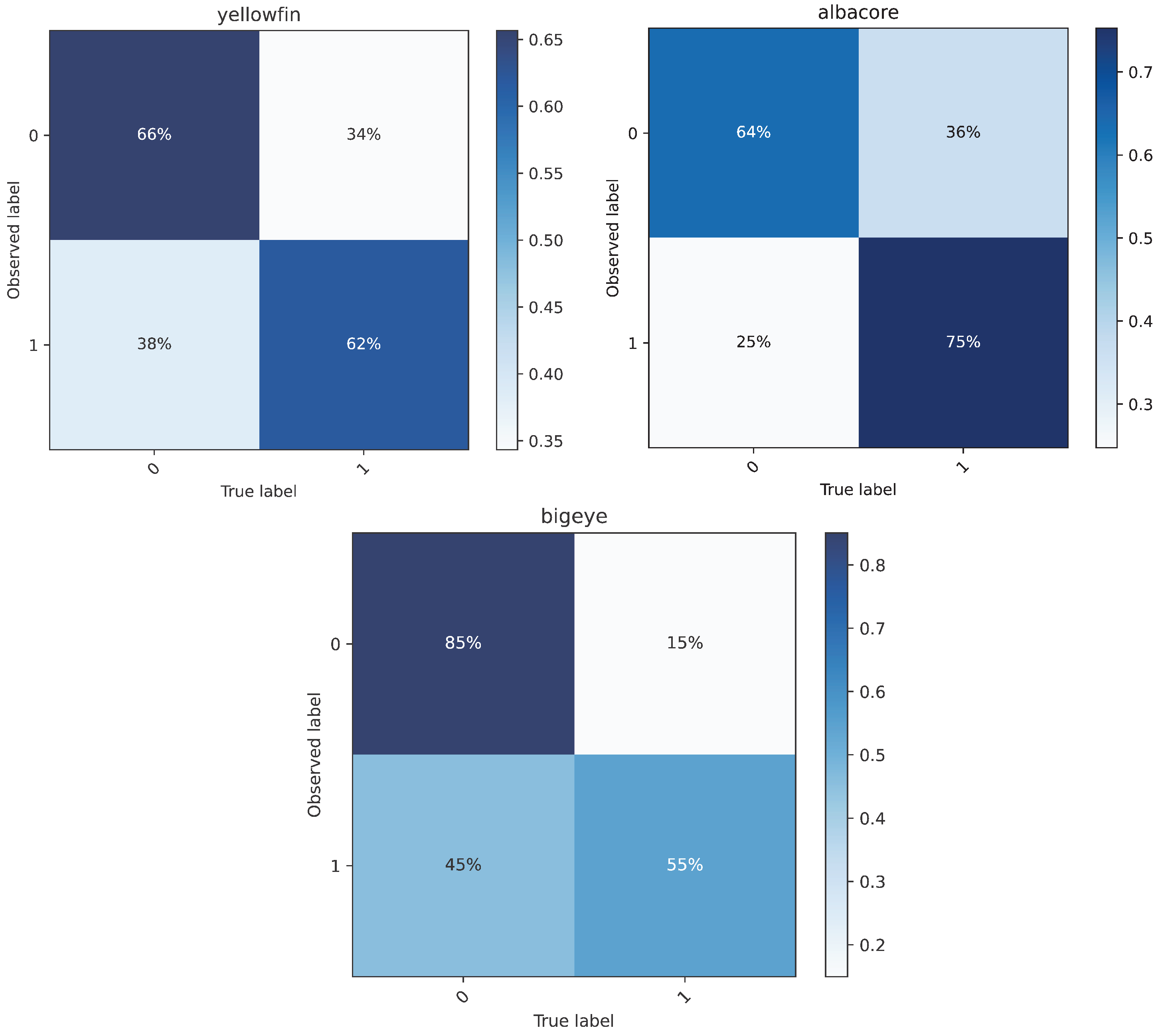
As shown in Table 2 and Figure 1, the Random Forest model is used to probe the noise in the yellowfin tuna, albacore tuna, and bigeye tuna datasets in the tropical waters of the Atlantic Ocean, respectively. In detail, yellowfin tuna as bycatch has the most zero-catch samples compared to the other two species, with 50.76% of the dataset, but 66% of these zeros were consistent with the true labels, and 53.77% of the zeros are judged to the noise, whereas, 38% of the non-zero samples are noise. About albacore tuna, also by-catch, the total number of zero-catch samples is smaller than for yellowfin tuna, the proportion of noise in zeros is also lower, at 43.20%. About bigeye tuna, which is the main catch, the reason why the percentage of zeros in the samples is only 5.05% is because the first quantile of CPUE in bigeye tuna dataset is 5, greater than 0, then labels equal to 0 are not represent that its CPUE equal to 0. Due to the scarcity of zero-catch data in bigeye tuna dataset, non-zero samples became the major factor interfering with fishery forecasts, 45% of the non-zero samples were determined to be noise, and the most dominant source of noise in the dataset.

In summary, whether for by-catch or main catch, zero-catch samples are not necessarily completely abnormal, and non-zero samples are not always normal, especially in the main catch. While abnormal samples certainly interfere with model training and prediction, uniformly modifying the labels of zero-catch samples will also affect the model’s forecasting performance seriously.

3.3.2. Forecasting performance

Unlike the previous subsection which will treat the entire dataset for noise detection, this subsection uses 75% of the samples in the dataset for model training and the remaining 25% of the samples for testing the model’s forecasting performance. In order to exclude the effect of repeated learning of samples in the test set on the forecasting performance, we first estimate the joint distribution of noisy samples and true samples in the training and test set[18] using two independent models and repair the noisy samples, and then use the third model to train on the repaired training set and assess the forecasting performance on the test set.

In order to validate the model universality of the anomalous sample detection method proposed in this paper and its effectiveness for the performance enhancement of fishery forecasting, we use three classical machine learning models (Random Forest, Support Vector Machine[19], and XGBoost[20]) to carry out the task of forecasting three species of tuna under the case of binary classification. The classical models are chosen because it is important to exclude as much as possible the positive impact of the generalization ability of the model structure on the performance of fishery forecasting, and to highlight the effectiveness of the anomalous sample detection method we proposed. In addition, although a variety of fishery forecasting models are currently available, the rate of improvement of model forecasting performance remains slow even stuck.

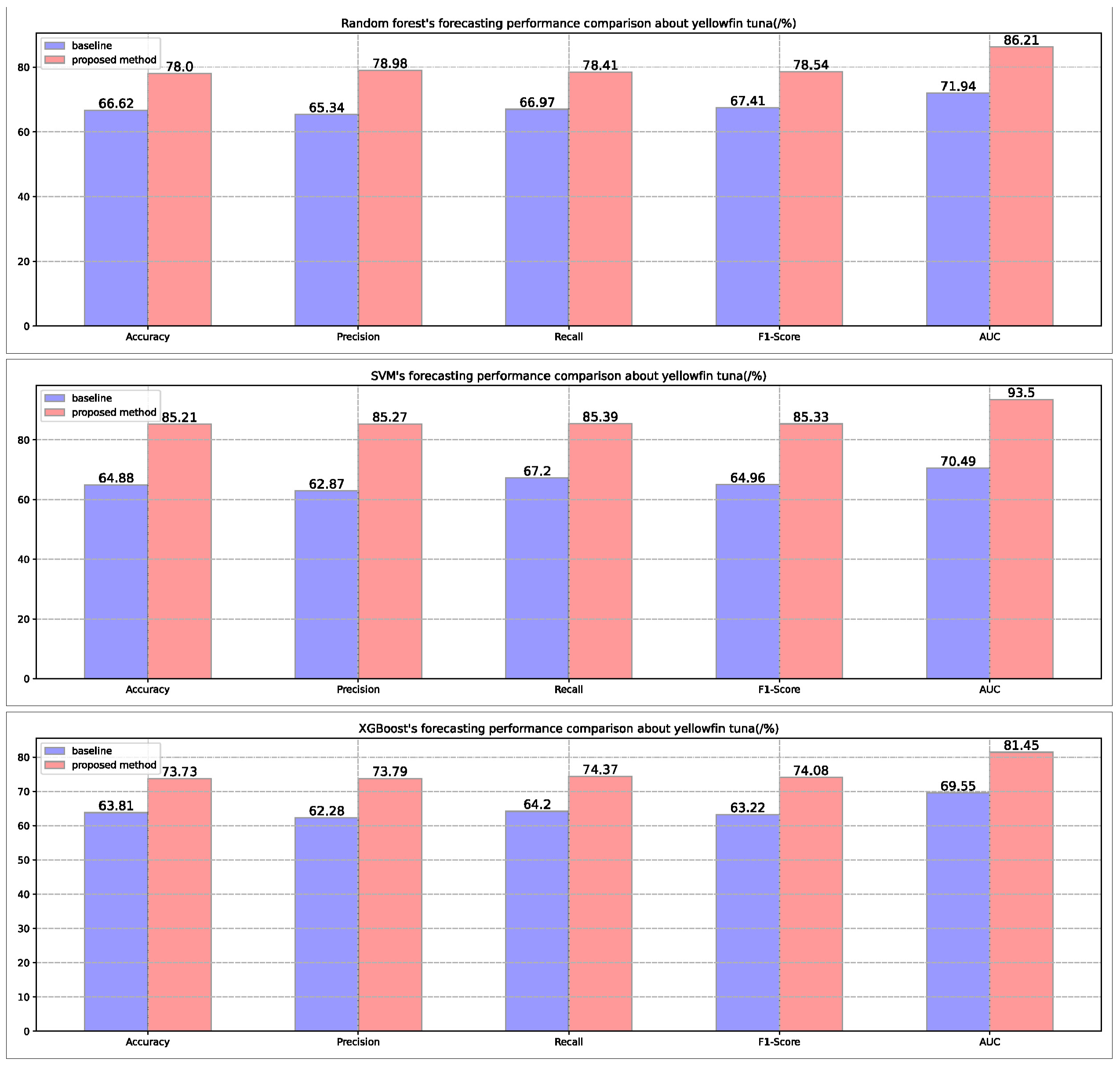
From the performance feedback of the three models on the three tuna datasets in Figure 2, Figure 3 and Figure 4, it can be seen that the performance of the three fishery forecasting models is still significantly improved when only the default hyperparameters are used, which verifies the model universality as well as the effectiveness of the proposed method.

Figure 2. The forecasting performance of three different kinds of model in the albacore tuna dataset.

Figure 2. The forecasting performance of three different kinds of model in the albacore tuna dataset.

Figure 3. The forecasting performance of three different kinds of model in the bigeye tuna dataset.

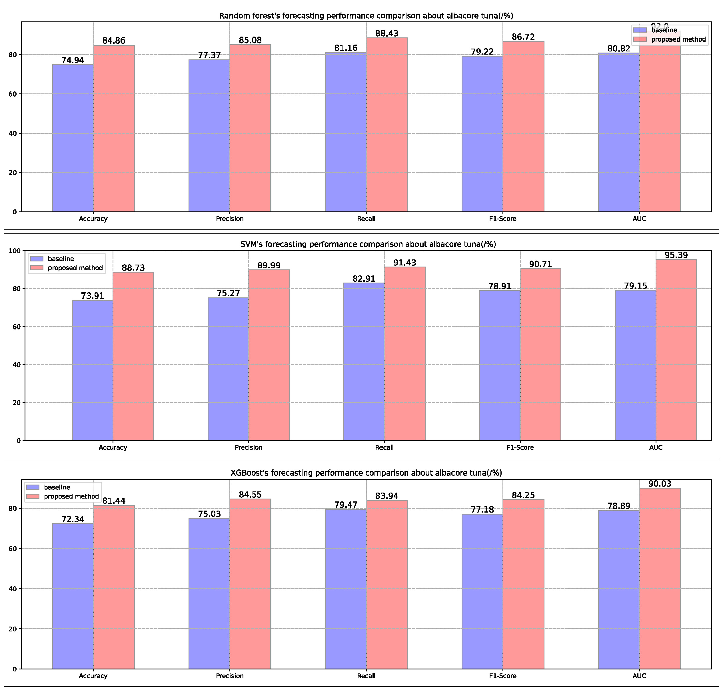
Figure 3. The forecasting performance of three different kinds of model in the bigeye tuna dataset.

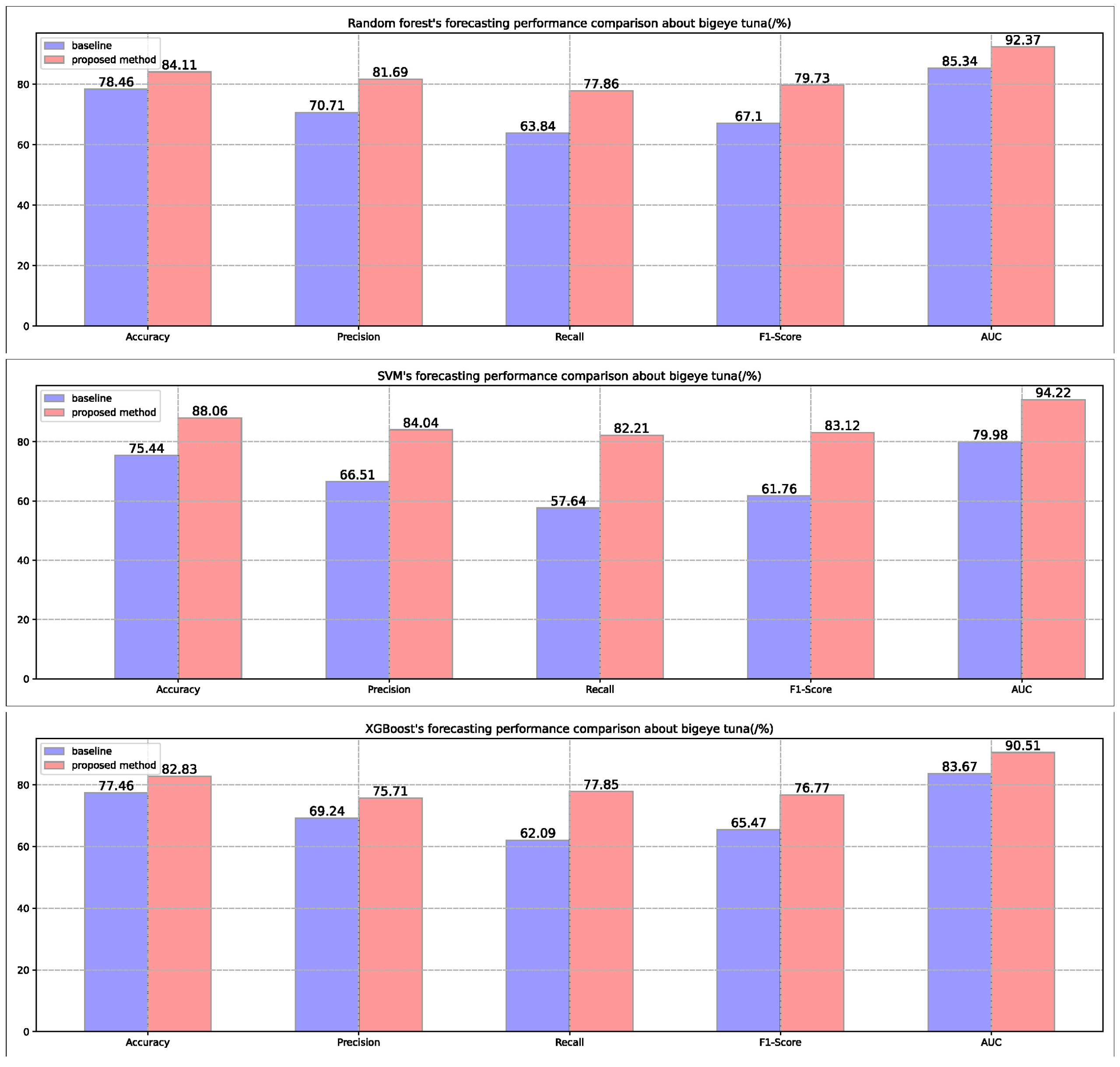
Figure 4. The forecasting performance of three different kinds of model in the yellowfin tuna dataset.

Figure 4. The forecasting performance of three different kinds of model in the yellowfin tuna dataset.

4. Discussion

In this paper, we take three species of tuna in the tropical waters of the Atlantic Ocean as experimental objects, and propose an anomalous fishery samples detection method applicable to both zero-vcatch samples and non-zero samples by utilizing the confident learning theory in learning with noisy labels. Compared with previous work for analyzing anomalous samples in fishery datasets (especially zero-catch samples), this paper proposes the concept of noise for the first time in the field of fishery forecasting, and succeeds in analyzing zero-catch samples and non-zero samples uniformly as noise. The analysis results show that there is a great heterogeneity among zero-catch samples (as well as among non-zero samples), i.e., a significant portion of zero-catch samples are corrected-labeled, revealing that the method of uniformly treating zeros in the previous studies is not conducive to improving the performance of fishery forecasting.

On the other hand, the method proposed in this paper quantitatively analyzes and detects a large number of anomalous samples in the non-zero samples, revealing that the large amount of noise in the non-zero samples is also an important reason hindering the improvement of the performance of fishery forecasting. The experimental results show that after detecting and repairing all the noises in the fishery dataset using the method we proposed, the forecasting performance of the three classical machine learning models (Random Forest, XGBoost, and Support Vector Machine) on the fishing dataset is significantly improved, confirming the effectiveness of the proposed method.

Although this paper has achieved some reasonable progress on the treatment of zero-catch problems by using the confident learning theory to unify zero-catch samples and non-zero samples together to solve the noise problem, it is possible that the fishery forecasting model has little ability to classify the hard samples to be poorly classified. Therefore, there are still some points that need to be further researched:

(1)we plan to design a strongly-coupled sample-denoising method by combining the confident learning theory and the hard negative mining theory[21] at the next stage, which can enable the model to exclude the interference of noisy samples while can improve the robustness and classification ability of itself for difficult samples, so as to obtain higher level.

(2)The confident learning theory adopted in our method can only do the preliminary quantitative analysis of the noise samples, and in the future, we plan to further expand the theory to quantitatively analyze the heterogeneity among zero-catch samples (as well as non-zero samples), such as quantifying the noise content of each noise sample and the signal-to-noise ratio of the dataset, or analyzing the causes of the anomalous samples through the expression of the environmental factors at the deeper level. In this way, the performance of the noise detection method for fishery data under the framework of learning with noisy labels can be improved.

References

- Maunder, N.; Punt, E. Standardizing catch and effort data: a review of recent approaches. Fish Res 2004, 70, 141–159. [Google Scholar] [CrossRef]
- Tian, S.; Chen, Y.; Chen, X.; et al. Impacts of spatial scales of fisheries and environmental data on CPUE standardization. Mar Freshwater Res 2009, 60, 1273–1284. [Google Scholar] [CrossRef]
- Campbell, A. CPUE standardizations and the construction of indices of stock abundance in a spatially varying fishery using general linear models. Fish Res 2004, 70, 209–227. [Google Scholar] [CrossRef]
- Campbell, A.; Tuck, G.; Tsuji, S.; Nishida, T. Indices of abundance for southern blue-fin tuna from analysis of fine-scale catch and effort data. Working Paper SBFWS/96/16 Presented at the Second CCSBT Scientific Meeting, Hobart, Australia, August 26–September 6, 1996.
- Shono, H. Application of the Tweedie distribution to zero-catch data in CPUE analysis. Fish Res 2008, 93, 154–162. [Google Scholar] [CrossRef]
- Thorson, T.; Ward, J. Accounting for space–time interactions in index standardization models Fish Res 2013, 147, 426–433. 147.
- Ralston, S.; Dick, J. The status of black rockfish (Sebastes melanops) off Oregon and northern Washington in 2003. Stock Assessment and Fishery Evaluation, Pacific Fishery Management Council, Portland, Oregon, America, 2003.
- Lambert, D. Zero-inflated Poisson regression, with an application to defects in manufacturing. Technometrics 1992, 34, 1–14. [Google Scholar] [CrossRef]
- Kawakita, M.; Minami, M.; Eguchi, S.; Lennert, E. An introduction to the predictive technique AdaBoost with a comparison to generalized additive models. Fish Res 2005, 76, 328–343. [Google Scholar] [CrossRef]
- Northcutt, G.; Jiang, L.; Chuang, L. Confident learning: Estimating uncertainty in dataset labels. JAIR 2021, 70, 1373–1411. [Google Scholar] [CrossRef]
- Song, L.; Li, T.; Zhang, T.; et al. Comparison of machine learning models within different spatial resolutions for predicting the bigeye tuna fishing grounds in tropical waters of the Atlantic Ocean. Fisheries Oceanography 2023, 18, 1–18. [Google Scholar] [CrossRef]
- Northcutt, G.; Jiang, L.; Chuang, L. Feng, Y.; Chen, X.; Gao, F.; Liu, Y. Impacts of changing scale on Getis-Ord Gi* hotspots of cpue: A case study of the neon flying squid (ommastrephes bartramii) in the northwest pacific ocean. Acta Oceanologica Sinica 2018, 37, 67–76. [Google Scholar]
- Akinwande, O.; Dikko, G.; Samson, A. Variance inflation factor: As a condition for the inclusion of suppressor variable(s) in regression analysis. Open Journal of Statistics 2015, 5, 754–767. [Google Scholar] [CrossRef]
- Wang, Y.; Ma, X.; Chen, Z.; Luo, Y.; Yi, J.; Bailey, J. Symmetric cross entropy for robust learning with noisy labels. ICCV 2019, 322–330. [Google Scholar]
- Han, B.; Yao, Q.; Yu, X.; Niu, G.; Xu, M.; Hu, W.; Tsang, I.; Sugiyama, M. Co-teaching: Robust training of deep neural networks with extremely noisy labels. NeurIPS 2018. [Google Scholar]
- Guo, C.; Pleiss, G.; Sun, Y.; Weinberger, Q. On calibration of modern neural networks. ICML 2017. [Google Scholar]
- Breiman, L. Random forests. Machine Learning 2001, 45, 5–32. [Google Scholar] [CrossRef]
- Northcutt, C. G.; Athalye, A.; Mueller, J. Pervasive label errors in test sets destabilize machine learning benchmarks. ICLR 2021. [Google Scholar]
- Cortes, C.; Vapnik, V. Support vector networks. Machine Learning 1995, 20, 273–297. [Google Scholar] [CrossRef]
- Chen, T.; Guestrin, C. XGBoost: A Scalable Tree Boosting System. ACM SIGKDD 2016. [Google Scholar]
Disclaimer/Publisher’s Note: The statements, opinions and data contained in all publications are solely those of the individual author(s) and contributor(s) and not of MDPI and/or the editor(s). MDPI and/or the editor(s) disclaim responsibility for any injury to people or property resulting from any ideas, methods, instructions or products referred to in the content. |
© 2023 by the authors. Licensee MDPI, Basel, Switzerland. This article is an open access article distributed under the terms and conditions of the Creative Commons Attribution (CC BY) license (http://creativecommons.org/licenses/by/4.0/).
Copyright: This open access article is published under a Creative Commons CC BY 4.0 license, which permit the free download, distribution, and reuse, provided that the author and preprint are cited in any reuse.