
Submitted:
30 August 2023
Posted:
31 August 2023
You are already at the latest version
Abstract
Among the various generalizations of persistent topology, the one based on rank functions and leading to indexing-aware functions appears to be particularly suited to catch graph-theoretical properties without the need for a simplicial construction and a homology computation. This paper defines and studies "simple" and "single-vertex" features in directed and undirected graphs, by which several indexing-aware persistence functions are produced, within the scheme of steady and ranging sets. The implementation of the "sink" feature and its application to trust networks provide an example of the ease of use and meaningfulness of the method.
Keywords:
Persistence
; categorical persistence functions
; indexing-aware persistence functions
; steady set
; ranging set
; weighted graph
; weighted digraph
1. Introduction
Computational topology and homological persistence provide swift algorithms to quantify geometrical and topological aspects of triangulable manifolds [1]. Let M be a triangulable manifold, given a continuous function , persistent homology consists in studying the evolution of homological classes throughout the sublevel-set filtration induced by f on M. Indeed, in this context, the word persistence refers to the lifespan of homological classes along the filtration. In intuitive terms, this procedure allows us to see M using f as a lens capable of highlighting features of interest in M.
Many extensions and generalizations of topological persistence aim to augment the field of application of persistent homology. Such generalizations allow for studying objects different than triangulable manifolds, maintaining the valuable properties granted by the persistent homology framework, e.g., stability [2], universality [3], resistance to occlusions [4], computability [5].
In most cases, generalizations of persistent homology can be attained in two ways. On the one hand, it is possible to define explicit mappings from the object of interest to a triangulable manifold preserving the properties of the original object, see, e.g., [6]. On the other hand, theoretical generalizations aim to extend the definition of persistence to objects other than triangulable manifolds and functors other than homology. These generalizations come in many flavors that we shall briefly recall in Section 2.1. Here, we shall consider the rank-based persistence framework and its developments and applications detailed in [7,8,9]. This framework revolves around an axiomatic approach, that yields usable definitions of persistence in categories such as graphs and quivers, without requiring the usage of auxiliary topological constructions.
In the current manuscript, following the approach described in [9,10], we provide strategies to compute rank-based persistence on weighted graphs (either directed or undirected). Weighted (di)graphs are widely used in many real-world scenarios ranging from analysis of interactions in social networks to context-based recommendation. Modern machine learning provides specific neural architectures to process directed graphs, e.g., [11,12,13]. As neural networks assure maximum flexibility by learning directly from training data, graph theory offers a plethora of invariants that—albeit static—can be leveraged as descriptors of directed, weighted networks [14,15,16]. We provide an algorithmic approach to encode such features as persistence diagrams carrying compact information that can be leveraged complementarily or even be integrated in modern neural analysis pipelines.
Organization of the paper
Section 2 briefly outlines various generalizations of persistence, and the current methods taking advantage of persistent homology on graphs and directed graphs (digraphs). Section 3 recalls the essential concepts for the generalized theory of persistence used in this manuscript. Namely, categorical and indexing-aware persistence functions. These functions are based on graph-theoretical features. In particular, we introduce the concept of simple features in Section 4, and single-vertex features in Section 5. This latter class of features yields plug-and-play methods for applications: we provide an implementation of single-vertex feature persistence in Section 6, and apply it in the context of trust networks. Section 7 concludes the paper.
2. State of the art
Oftentimes, modern datasets can be endowed with a network-like structure. At the same time, topological persistence, thanks to its aforementioned mathematically provable properties, proved to be a valuable tool in many applications. Thus, generalizations of topological persistence and its adaptations to objects such as graphs and directed graphs are lively research lines.
2.1. Generalizations of persistence
The keystone of persistence theory is classically the persistence module, i.e. a functor from the category to the category of modules on a fixed ring (generally a field), that catches the essential features of a filtered topological space or simplicial complex. As hinted previously, the filtration is mostly constituted by the nested sublevel-sets of a real filtering function. The modules are the images of the linear maps induced in homology by the inclusions. This setting provides great modularity: different filtering functions may catch different features [17]. The most used filtering function is the ball radius in building Vietoris-Rips or Čech complexes out of sampled objects [18].
Extensions of the classical persistence theory offer much greater flexibility. The first generalization was the passage from a single-parameter to multi-parameter filtering functions [19,20] and to different ranges for the filtering function [21]. However, we believe that the most impactful generalizations are in categorical terms. In [22], persistence theory is extended to functors from to any Abelian category, in particular for what concerns the interleaving distance. This distance is also investigated in [3] for multidimensional domains, and extended in [23] to functors from a poset to an arbitrary category. Posets as domains are studied in [24] and [25] for a generalized notion of persistence diagram. The extension on which the present paper is based is exposed in [7] and aims to widen the range of phenomena that can give rise to persistence diagrams. This is done via rank functions which generalize the dimension of homology modules in classical persistence.
2.2. Persistent homology for graphs and digraphs
Data frequently come in the form of graphs or digraphs, and researchers were often attracted by the possibility of applying persistence to the analysis of networks. The classical strategy consists in building a filtered simplicial complex from a weighted graph, and then compute persistent homology. This can be done in several ways [6]. Of course, the most direct way is to consider the graph itself as a 1-dimensional simplicial complex (or CW-complex if loops and multiple edges are allowed). This is done, e.g., in [26], where a connection between Laplacian, persistence, and network circuit graphs is drawn. [27] does persistence on discrete curvature for the evaluation of graph generative models. The clique complex is also a very natural way of transforming a graph into a possibly multidimensional complex. This latter construction is leveraged in [28] for the study of deep neural networks, in [29] for the analysis of the dynamics of scientific knowledge, and also in [30] and [31] (among many others) for the representation and study of the human connectome. Persistent homology of clique-communities complexes is applied to the study of general types of complex networks in [32,33]. Other constructions of simplicial complexes—e.g. independent sets, neighborhoods, dominating sets—are also discussed and utilized in applications but, to the best of our knowledge, not in connection with persistence.
The construction of simplicial complexes from digraphs poses similar but not coinciding problems than its undirected counterpart. In [34] directed cliques are used to investigate the structural and functional topology of the brain. A differently flavored homology is built in [35,36], where the role of simplices is played by directed paths. Directed paths are also at the base of an application of Hochschild homology [37, Ch.1]—through the use of connectivity digraphs and within the framework of [7]—for a new persistence homology for digraphs in [38].
3. Graph-theoretical persistence
To the best of our knowledge, current applications of persistence to graphs and digraphs leverage homology of some kind. Here, we provide a non-necessarily-homological approach to the study of graphs and digraphs. We recall the basic notions of the extension of topological persistence to graph theory introduced in [7,8]. For an encompassing view on classical topological persistence, we refer the reader to [39,40].
3.1. Categorical persistence functions
Definition 1.
[7, Def. 3.2] Let be a category. We say that a lower-bounded function is a categorical persistence function if, for all , the following inequalities hold:
- and
With , the graphs of such functions have the appearance of superimposed triangles typical of Persistent Betti Number functions [39, Sect. 2], so they can be condensed into persistence diagrams [7, Def. 3.16].
In the remainder, we shall write “(di)graph” for “graph (respectively digraph)”, extending this notation to cases such as sub(di)graph et similia. Symmetrically and when no confusion arises, we shall denote with the category or the category , with monomorphisms as morphisms. We shall use the noun edge for edges of a graph and arcs of a digraph.
Filtered (di)graphs are pairs consisting of a (di)graph and a filtering function on the edges and extended to each vertex as the minimum of the values of its incident edges. For any , the sublevel (di)graph (briefly if no confusion occurs) is the sub(di)graph induced by the edges e such that .
Definition 2.
[8, Def. 5] The natural pseudodistance of filtered (di)graphs and is
where is the set of (di)graph isomorphisms between G and .
Let p be a categorical persistence function on , , any filtered (di)graphs, , the respective persistence diagrams, and d be the bottleneck distance [39, Sect. 6][7, Def. 3.24].
Definition 3.
[8, Sect. 2] The categorical persistence function p is said to be stable if the inequality
holds. Moreover, the bottleneck distance is said to be universal with respect to p, if it yields the best possible lower bound for the natural pseudodistance, among the possible distances between and , for any , .
3.2. Indexing-aware persistence functions
The difference between any of the categorical persistence functions introduced in [8] and the functions of the present subsection (presented originally in [9]) is that the former comes from a functor defined on , while the latter strictly depends on the filtration, thus descending from a functor defined on .
Definition 4.
[9, Def. 5] Let p be a map assigning to each filtered (di)graph a categorical persistence function on , such that whenever an isomorphism between and compatible with the functions exists.
All the resulting categorical persistence functions are called indexing-aware persistence functions (ip-functions for brevity). The map p itself is called an ip-function generator.
Definition 5.
[9, Def. 6, Prop. 1] Let p be an ip-function generator on . The map p itself and the resulting ip-functions are said to be balanced if the following condition is satisfied. Let be any (di)graph, f and g two filtering functions on G, and and their ip-functions. If a positive real number h exists, such that , then for all the inequality holds.
Proposition 6. [9, Thm. 1] Balanced ip-functions are stable.
We now recall our main ip-function generators: steady and ranging sets.
Definition 7.
[9, Def. 8] Given a (di)graph , any function is called a feature. Conventionally, for we set in a sub(di)graph if .
Remark 8.
The second part of Def. 7 was added for use in some of the following proofs.
Let be a feature.
Definition 9.
[9, Def. 8] We call -set any such that . In a weighted (di)graph G, we shall say that is an -set at level if it is an -set of .
Definition 10.
[9, Def. 9] We define the maximal feature associated with as follows: for any , if and only if and there is no such that and .
Definition 11.
We call X a ranging-set (r-set) at if there exist levels and at which it is an -set.
Let be the set of s-sets at and let be the set of r-sets at .
Definition 12.
[9, Def. 11] For any filtered (di)graph we define (resp. ) as the function which assigns to , the number (resp. ).
We denote by and the maps assigning and respectively to .
Proposition 13. [9, Prop. 2] The maps and are ip-function generators.
The next definition will be generalized in Section 4.
Definition 14.
[9, Def. 13] We say that a feature is monotone if
- for any (di)graphs , and any , in implies in
- in any (di)graph , for any , implies .
Proposition 15. [9, Prop. 3] If is monotone, then
Proposition 16. [9, Prop. 4] If is monotone, then the ip-function generators are balanced.
4. Simple features
We now define a class of features extending the class of monotone features (Def. 14).
Definition 17.
Let be a (di)graph. A feature is said to be simple if, for and for sub(di)graphs the following condition holds:
if in and in , then in
For the remainder of this section, let be a weighted (di)graph, , and a simple feature in G.
Lemma 18.
Let . Then, either there is no value u for which in , or in for all , where is the lowest value u such that in the sub(di)graph one has in , and is either the lowest value for which in or .
Proof.
Assume that there is at least a value such that in . There surely are values w such that in : at least the values beneath the minimum attained by f; let be such that in ; for any set , , . Then, by Def. 17, in . So between two values for which there cannot be one such that . □
Definition 19.
The interval of Lemma 19, i.e. the widest interval for which in , is called the -interval of X in .
Proposition 20.
Proof.
By Lemma 19, since and would differ only if, for at least one set X, there were values for which in and in but in . □
It is easy to prove that the following features are simple.
Example 21.
For a graph G, the (rather trivial) feature for which if and only if X is a singleton containing a vertex of a fixed degree d is simple. Also the feature for which if and only if X is a singleton containing a vertex whose degree is is simple, with half-lines as -intervals. Analogous features are defined for a digraph in terms of indegree and outdegree.
Example 22.
For a (di)graph G, if and only if X is a set of vertices inducing a connected subgraph (resp. a strongly connected subdigraph) of G. is simple and its -intervals are half-lines.
Example 23.
For a (di)graph G, if and only if X is a set of vertices inducing a connected component (resp. a strong component) of G. is simple; for the -interval of a set X, the value either is or the value at which some other vertex joins the component (resp. strong component) induced by X.
Proposition 24.
For a (di)graph G, any monotone feature is simple.
Proof.
Let be a (di)graph and be a monotone feature. For and assume that in and in . By condition 1 of Def. 14, (recall the convention of Def. 7), so also and in . □
Lemma 25.
Let be filtering functions on a (di)graph G, and assume that there exists a positive real number h such that . Then, for real numbers such that , the sublevel (di)graph is a sub(di)graph of and is a sub(di)graph of .
Proof.
For any , if then ; analogously, if then . □
The following Proposition generalizes Prop. 16 (i.e. [9, Prop. 4]) with essentially the same proof.
Proposition 26.
The ip-function generators are balanced, hence stable.
Proof.
With the same hypotheses as in Lemma 25, let be such that in at all levels , with . For any we now show that in . In fact, by Prop. 25 is a sub(di)graph of , which is a sub(di)graph of . Since is simple and both in and in , we necessarily have that in . Therefore there is an injective map (actually an inclusion map) from to , therefore . Stability comes from Prop. 6. □
Remark 27.
The maximal version of a simple feature (Def. 10) is generally not simple: an example is the feature identifying independent sets of vertices, which is monotone (hence simple) while the ip-functions corresponding to its maximal version are not balanced ([9, Sect. 2.4, Appendix, Fig.
14, Fig. 15]), so is not simple. Still, some are.
Proposition 28.
For a (di)graph G, the feature [9, Sect. 2.4], i.e. such that if and only if X is a maximal matching, is simple.
Proof.
A matching of a graph is a matching also of any supergraph. If, for , we have in and in , this means that X is a maximal matching in but is not in . There are only two ways of not being a maximal matching in : either or contains a matching . The latter is impossible because in that case, X would not be maximal in either. So and in . □
Two variations on the notion of matching for digraphs are the following.
Example 29.
For a digraph , if and only if X is a set of arcs, any two of which have neither the same head nor the same tail. Such a set X is said to be path-like.
Example 30.
For a digraph , if and only if X is a set of arcs, such that for any two of them the head of one is not the tail of the other. Such a set X is said to be path-less.
Proposition 31.
The features and are monotone, hence simple.
Proof.
Straightforward. □
Proposition 32.
The features and are simple.
Proof.
Same as for Prop. 28. □
5. Single-vertex features
Some features are of particular interest in applications: those that may be true on singletons consisting of vertices. They can be categorized as point-wise if they depend on the single vertex, local if they depend on the k-neighborhood of the vertex for some k, or global if they depend on the whole (di)graph.
Example 33.
See Example 21 for examples of point-wise features.
Example 34.
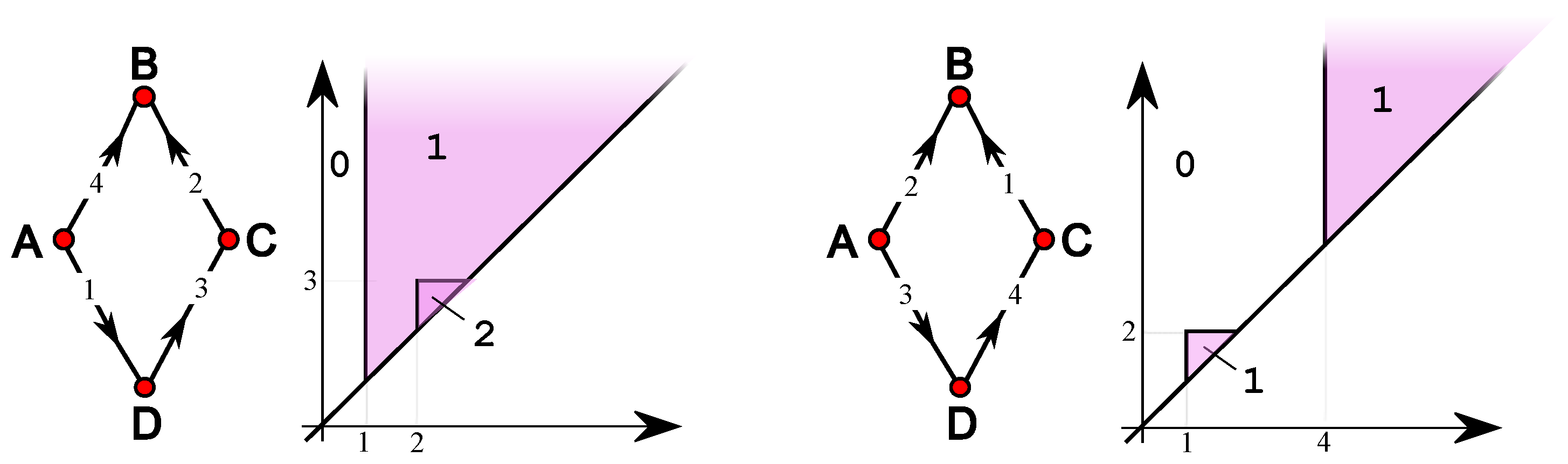
Another point-wise feature for a digraph G is , for which if and only if X consists of a single vertex (that we call a source) whose outdegree is larger than its indegree. An analogous feature identifies a sink, where the indegree exceeds the outdegree. Variations on these features can be built by specifying that the outdegree (respectively indegree) exceeds a fixed fraction of the total degree of the vertex. The usual example with its ip-functions (middle) and is shown in Figure 2. and are not balanced: see the Appendix.
Example 35.
Example 36.
In [10, Sect. 4.1.4] a local feature is defined for the graph representing a gray-tone image, where each vertex is a pixel and is adjacent to each of its eight neighboring pixels. The filtering function maps each edge to the minimum of the intensities of the incident pixels. The feature (short: ) maps each vertex v to if and only if more than m and less than n pixels at distance have intensity . The function is proved to be balanced [41, Thm. 4.3.1].
Example 37.
A global feature in a digraph G is for which if and only if X consists of a vertex (that we call a root) from which there is a directed path to each vertex of the connected component containing it. Figure 3 shows the same weighted digraph of the previous examples, with its ip-functions (middle) and . and are not balanced: see the Appendix.
6. Computational Experiments
Large, directed, weighted graphs are largely used in representing context-based rating, from recommendation engines to trust networks.
We implemented the single-vertex features described in Section 5 as part of the Generalized Persistence Analysis Python package available at https://github.com/LimenResearch/gpa.
6.1. Algorithm
We consider a directed, weighted graph and apply a transformation function on the weights defined on its edges. Transformed weights induce a sublevel-set filtration. See Figure 4. For each sublevel set, we compute a single-vertex feature (sink in Figure 4). Finally, we compute the persistence in terms of the considered single vertex feature, realized by each vertex throughout the filtration. Thus, the persistence associated to each vertex is the largest interval where the feature holds, as detailed in [9].
The software interface we adopted for this algorithm is provided at https://github.com/LimenResearch/gpa/tree/master/gpa/examples/bitcoin/bitcoin.py.The user instantiate a directed weighted graphs, specify a transformation function to be applied to the weights to obtain the filtration, and finally chooses the single-vertex feature among the implemented ones, namely sources and sinks. These features are implemented by adding two simple methods to the WeightedGraph class for the computation of the feature itself, and to apply the computation to each step of the filtration.
6.2. Datasets
The OTC and Bitcoin Alpha datasets consist of user-to-user trust networks of Bitcoin traders on the OTC and Alpha platform, respectively [42]. Users can express a vote of trust on other users by assigning them a integer rating varying from (fraudulent user) to 10 (completely trustworthy), excluding the value 0. We utilized the data and ground truth provided in https://github.com/horizonly/Rev2-model/tree/master. There, fraudulent and trustworthy users are identified by considering the platform founders votes.
6.3. Results
We computed the steady persistence of the source single-vertex feature considering the sublevel set filtration induced on the Bitcoin Alpha network by the function
where is the set of all weights defined on the network’s edges.
For each sublevel of the filtration and each of its nodes, we say that a vertex v is a sink if the sum of the weights of its in-edges is larger the sum of the weights defined on its out-edges. In symbols:
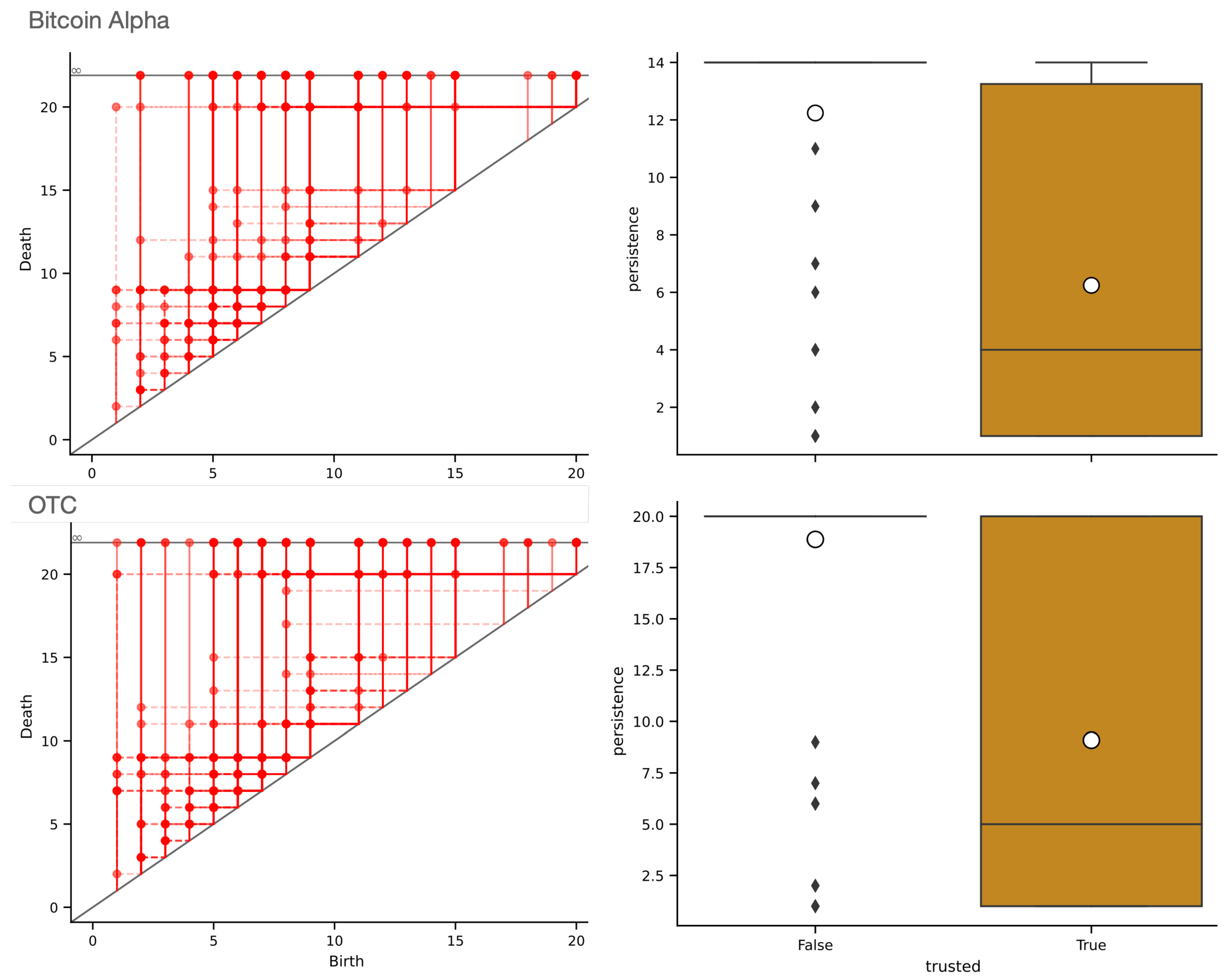
This computation gives rise to the persistence diagram in Figure 5 (left panel). The persistence associated with the networks’ nodes allows us to draw the histogram of the values associated with trustworthy and fraudulent users, respectively, See Figure 5 (right panel). The histogram reveals how nodes representing fraudulent users attain high persistence levels (with mean and most of them being represented by cornerline in the persistence diagram, i.e., points with infinite persistence, as showcased in Figure 5), while trustworthy users’ persistence is typically finite with mean and median 4.
7. Conclusions
The availability of massive data represented as graphs expedited the development of computational methods specialized in handling data endowed with the complex structures arising from pairwise interactions.
We provide a computational recipe to generate compact representations of large networks according to graph-theoretical features or custom properties defined on the networks’ vertices. To do this, we leverage a generalization of topological persistence adapted to work on weighted (di)graphs. In this framework, we widen the notion of monotone feature on (di)graphs—i.e., feature respecting inclusion—and thus, well suited to generate filtrations and persistence diagrams. Simple features are a special case of features, whose value can change from true to false only once in a filtration of a (di)graph. We prove that in a (di)graph any monotone feature is simple and that simple features give rise to stable indexing-aware persistence functions. We then provide examples of simple features. Turning our attention to application, single-vertex features allow the user to compute the persistence of a weighted (di)graph for any feature, focused on singletons. There, we provide several examples, characterizing single-vertex features as point-wise, local, or global descriptors of a network.
Computational experiments—supporting our belief that single-vertex feature can be easily integrated in applications—show how the sink feature characterizes the users of trust networks. When considering the persistence of sink vertices, fraudulent users are, in the majority of cases, represented by half-lines with infinite persistence, while trusted users are associated with finite persistence. To replicate our results, we provide a Python implementation of the algorithm for the computation of single-vertex feature persistence integrating it in the package originally supporting [8,9].
We believe that straightforward implementation to compute local and global descriptors of networks arising from easily engineerable features can complement and help gaining control on current approaches based on artificial neural architectures and learned features.
Acknowledgments
Work performed under the auspices of INdAM-GNSAGA.
Appendix A. Unbalanced
The ip-function generators and are not balanced (Def. 5), as the weighted digraphs and of Figure A1 show. In fact, and . coincides with in this particular case.
Figure A1.
Left: and the corresponding . Right: and the corresponding .
The ip-function generators and are not balanced (Def. 5), as the weighted digraphs and of Figure A2 show. In fact, and . coincides with in this particular case.
Figure A2.
Left: and the corresponding . Right: and the corresponding .
References
- Otter, N.; Porter, M.A.; Tillmann, U.; Grindrod, P.; Harrington, H.A. A roadmap for the computation of persistent homology. EPJ Data Science 2017, 6, 1–38. [Google Scholar] [CrossRef]
- Cohen-Steiner, D.; Edelsbrunner, H.; Harer, J. Stability of persistence diagrams. Symposium on Computational Geometry; Mitchell, J.S.B.; Rote, G., Eds. ACM, 2005, pp. 263–271.
- Lesnick, M. The Theory of the Interleaving Distance on Multidimensional Persistence Modules. Foundations of Computational Mathematics, 2015; 1–38. [Google Scholar] [CrossRef]
- Di Fabio, B.; Landi, C. A Mayer–Vietoris formula for persistent homology with an application to shape recognition in the presence of occlusions. Foundations of Computational Mathematics 2011, 11, 499–527. [Google Scholar] [CrossRef]
- Malott, N.O.; Chen, S.; Wilsey, P.A. A survey on the high-performance computation of persistent homology. IEEE Transactions on Knowledge and Data Engineering 2022, 35, 4466–4484. [Google Scholar] [CrossRef]
- Bergomi, M.G.; Ferri, M.; Zuffi, L. Topological graph persistence. Communications in Applied and Industrial Mathematics 2020, 11, 72–87. [Google Scholar] [CrossRef]
- Bergomi, M.G.; Vertechi, P. Rank-based persistence. Theory and applications of categories 2020, 35, 228–260. [Google Scholar]
- Bergomi, M.G.; Ferri, M.; Vertechi, P.; Zuffi, L. Beyond Topological Persistence: Starting from Networks. Mathematics 2021, 9. [Google Scholar] [CrossRef]
- Bergomi, M.G.; Ferri, M.; Tavaglione, A. Steady and ranging sets in graph persistence. Journal of Applied and Computational Topology 2022, 1–24. [Google Scholar] [CrossRef]
- Bergomi, M.G.; Ferri, M.; Mella, A.; Vertechi, P. Generalized Persistence for Equivariant Operators in Machine Learning. Machine Learning and Knowledge Extraction 2023, 5, 346–358. [Google Scholar] [CrossRef]
- Monti, F.; Otness, K.; Bronstein, M.M. Motifnet: a motif-based graph convolutional network for directed graphs. In Proceedings of the 2018 IEEE Data Science Workshop (DSW). IEEE; 2018; pp. 225–228. [Google Scholar]
- Tong, Z.; Liang, Y.; Sun, C.; Rosenblum, D.S.; Lim, A. Directed graph convolutional network. arXiv 2020, arXiv:2004.13970. [Google Scholar]
- Zhang, X.; He, Y.; Brugnone, N.; Perlmutter, M.; Hirn, M. Magnet: A neural network for directed graphs. Advances in neural information processing systems 2021, 34, 27003–27015. [Google Scholar]
- Estrada, E. The structure of complex networks: theory and applications; Oxford University Press, USA, 2012.
- Zhao, S.X.; Fred, Y.Y. Exploring the directed h-degree in directed weighted networks. Journal of Informetrics 2012, 6, 619–630. [Google Scholar] [CrossRef]
- Yang, Y.; Xie, G.; Xie, J.; others. Mining important nodes in directed weighted complex networks. Discrete Dynamics in Nature and Society 2017, 2017. [Google Scholar] [CrossRef]
- Ferri, M. Persistent topology for natural data analysis – A survey. In Towards Integrative Machine Learning and Knowledge Extraction; Springer, 2017; pp. 117–133.
- Carlsson, G. Topology and data. Bull. Amer. Math. Soc. 2009, 46, 255–308. [Google Scholar] [CrossRef]
- Carlsson, G.; Singh, G.; Zomorodian, A. Computing Multidimensional Persistence. ISAAC; Dong, Y.; Du, D.Z.; Ibarra, O.H., Eds. Springer, 2009, Vol. 5878, Lecture Notes in Computer Science, pp. 730–739.
- Cerri, A.; Di Fabio, B.; Ferri, M.; Frosini, P.; Landi, C. Betti numbers in multidimensional persistent homology are stable functions. Mathematical Methods in the Applied Sciences 2013, 36, 1543–1557. [Google Scholar] [CrossRef]
- Burghelea, D.; Dey, T.K. Topological persistence for circle-valued maps. Discrete & Computational Geometry 2013, 50, 69–98. [Google Scholar]
- Bubenik, P.; Scott, J.A. Categorification of persistent homology. Discrete & Computational Geometry 2014, 51, 600–627. [Google Scholar]
- de Silva, V.; Munch, E.; Stefanou, A. Theory of interleavings on categories with a flow. Theory and Applications of Categories 2018, 33, 583–607. [Google Scholar]
- Kim, W.; Mémoli, F. Generalized persistence diagrams for persistence modules over posets. Journal of Applied and Computational Topology 2021, 5, 533–581. [Google Scholar] [CrossRef]
- McCleary, A.; Patel, A. Edit Distance and Persistence Diagrams Over Lattices. SIAM Journal on Applied Algebra and Geometry 2022, 6, 134–155. [Google Scholar] [CrossRef]
- Mémoli, F.; Wan, Z.; Wang, Y. Persistent Laplacians: Properties, algorithms and implications. SIAM Journal on Mathematics of Data Science 2022, 4, 858–884. [Google Scholar] [CrossRef]
- Southern, J.; Wayland, J.; Bronstein, M.; Rieck, B. Curvature filtrations for graph generative model evaluation. arXiv 2023, arXiv:2301.12906. [Google Scholar]
- Watanabe, S.; Yamana, H. Topological measurement of deep neural networks using persistent homology. Annals of Mathematics and Artificial Intelligence 2022, 90, 75–92. [Google Scholar] [CrossRef]
- Ju, H.; Zhou, D.; Blevins, A.S.; Lydon-Staley, D.M.; Kaplan, J.; Tuma, J.R.; Bassett, D.S. Historical growth of concept networks in Wikipedia. Collective Intelligence 2022, 1, 26339137221109839. [Google Scholar] [CrossRef]
- Sizemore, A.E.; Giusti, C.; Kahn, A.; Vettel, J.M.; Betzel, R.F.; Bassett, D.S. Cliques and cavities in the human connectome. Journal of Computational Neuroscience 2018, 44, 115–145. [Google Scholar] [CrossRef] [PubMed]
- Guerra, M.; De Gregorio, A.; Fugacci, U.; Petri, G.; Vaccarino, F. Homological scaffold via minimal homology bases. Scientific reports 2021, 11, 5355. [Google Scholar] [CrossRef]
- Rieck, B.; Fugacci, U.; Lukasczyk, J.; Leitte, H. Clique community persistence: A topological visual analysis approach for complex networks. IEEE Transactions on Visualization and Computer Graphics 2018, 24, 822–831. [Google Scholar] [CrossRef]
- Aktas, M.E.; Akbas, E.; Fatmaoui, A.E. Persistence homology of networks: methods and applications. Applied Network Science 2019, 4, 1–28. [Google Scholar] [CrossRef]
- Reimann, M.W.; Nolte, M.; Scolamiero, M.; Turner, K.; Perin, R.; Chindemi, G.; Dłotko, P.; Levi, R.; Hess, K.; Markram, H. Cliques of Neurons Bound into Cavities Provide a Missing Link between Structure and Function. Frontiers in Computational Neuroscience 2017, 11, 48. [Google Scholar] [CrossRef]
- Chowdhury, S.; Mémoli, F. Persistent path homology of directed networks. Proceedings of the Twenty-Ninth Annual ACM-SIAM Symposium on Discrete Algorithms. SIAM, 2018, pp. 1152–1169.
- Dey, T.K.; Li, T.; Wang, Y. An efficient algorithm for 1-dimensional (persistent) path homology. Discrete & Computational Geometry 2022, 68, 1102–1132. [Google Scholar]
- Loday, J.L. Cyclic homology; Vol. 301, Springer Science & Business Media, 2013.
- Caputi, L.; Riihimäki, H. Hochschild homology, and a persistent approach via connectivity digraphs. Journal of Applied and Computational Topology 2023, 1–50. [Google Scholar] [CrossRef]
- Edelsbrunner, H.; Harer, J. Persistent homology—a survey. In Surveys on discrete and computational geometry; Amer. Math. Soc.: Providence, RI, 2008; Vol. 453, Contemp. Math., pp. 257–282.
- Edelsbrunner, H.; Harer, J. Computational Topology: An Introduction; American Mathematical Society, 2009.
- Mella, A. Non-topological persistence for data analysis and machine learning. PhD thesis, Alma Mater Studiorum - Università di Bologna, Italy, 2021.
- Kumar, S.; Spezzano, F.; Subrahmanian, V.; Faloutsos, C. Edge weight prediction in weighted signed networks. In Proceedings of the 2016 IEEE 16th International Conference on Data Mining (ICDM). IEEE; 2016; pp. 221–230. [Google Scholar]
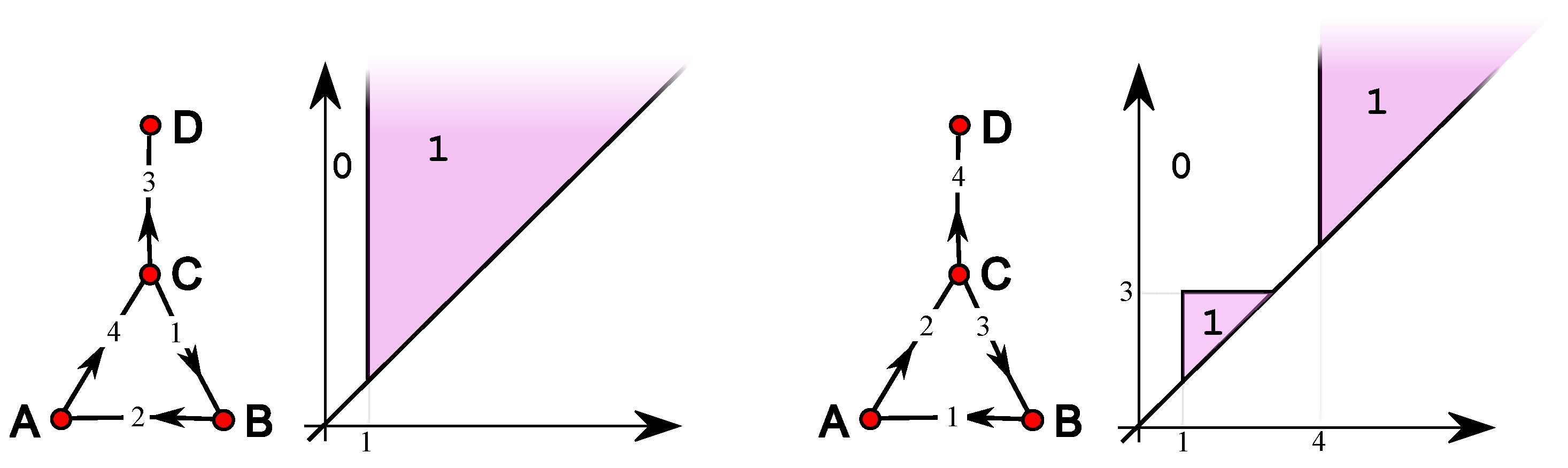
Figure 1.
A weighted digraph (left), its coinciding ip-functions and (middle) and its coinciding ip-functions and . Above, the filtration is shown.
Figure 1.
A weighted digraph (left), its coinciding ip-functions and (middle) and its coinciding ip-functions and . Above, the filtration is shown.
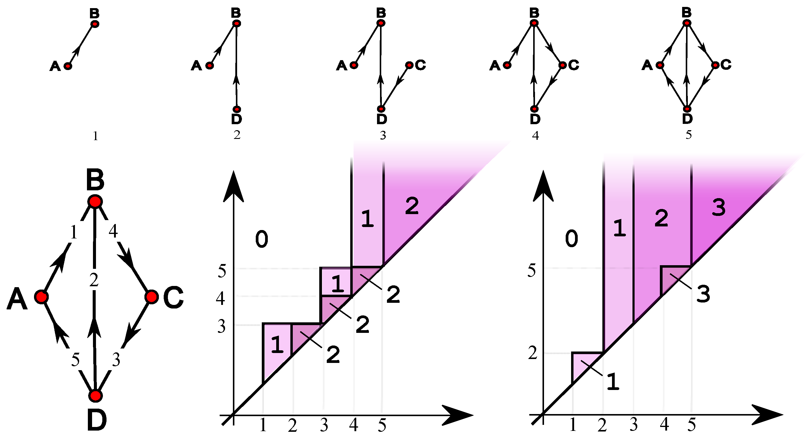
Figure 2.
A weighted digraph (left) and its ip-functions (middle) and (left).
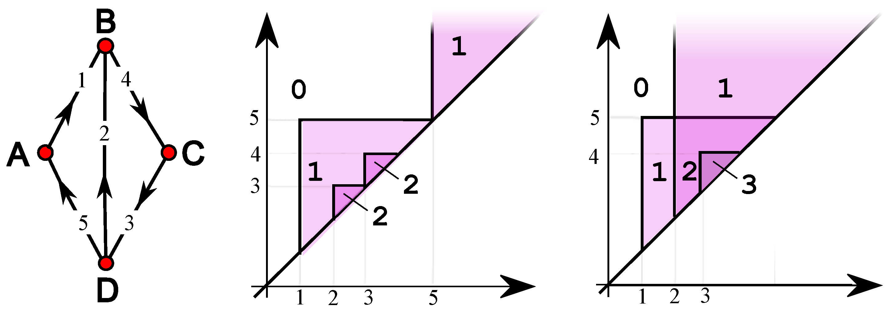
Figure 3.
A weighted digraph (left) and its ip-functions (middle) and .
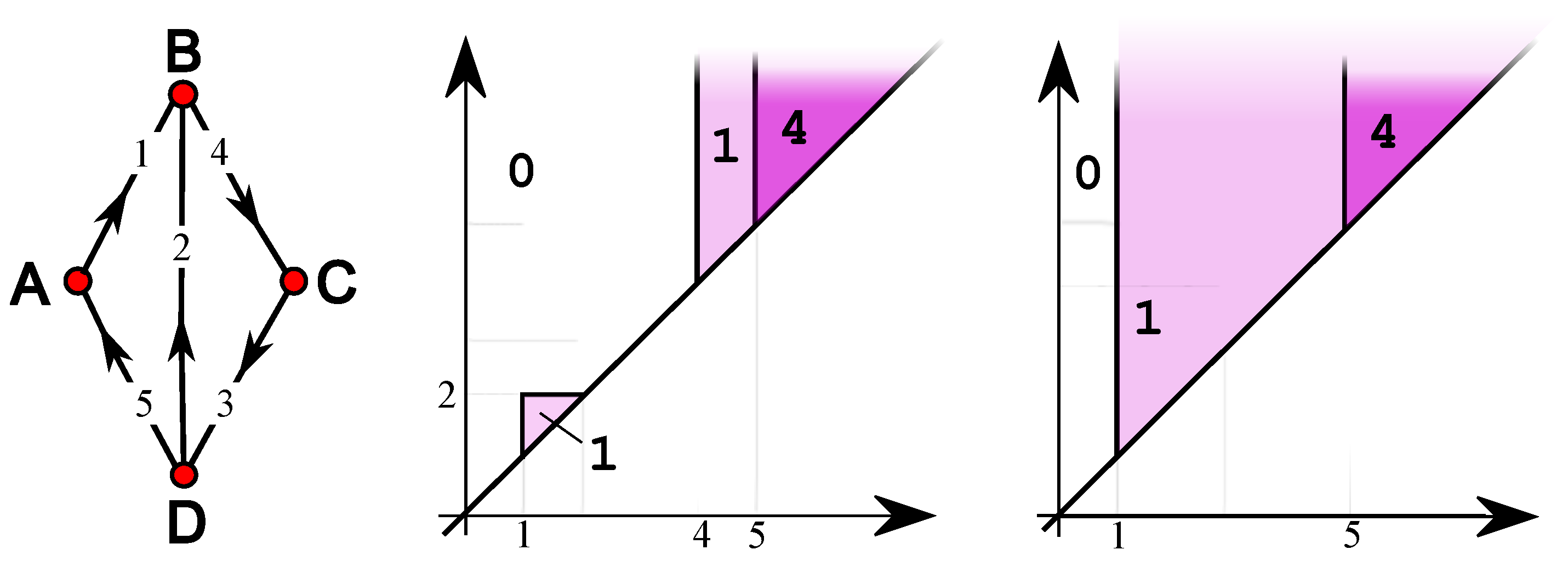
Figure 4.
Algorithmic flow. A directed weighted graph is mapped to a filtration (induced by transformed weights). Then, persistence is computed according to a given single-vertex feature.
Figure 4.
Algorithmic flow. A directed weighted graph is mapped to a filtration (induced by transformed weights). Then, persistence is computed according to a given single-vertex feature.
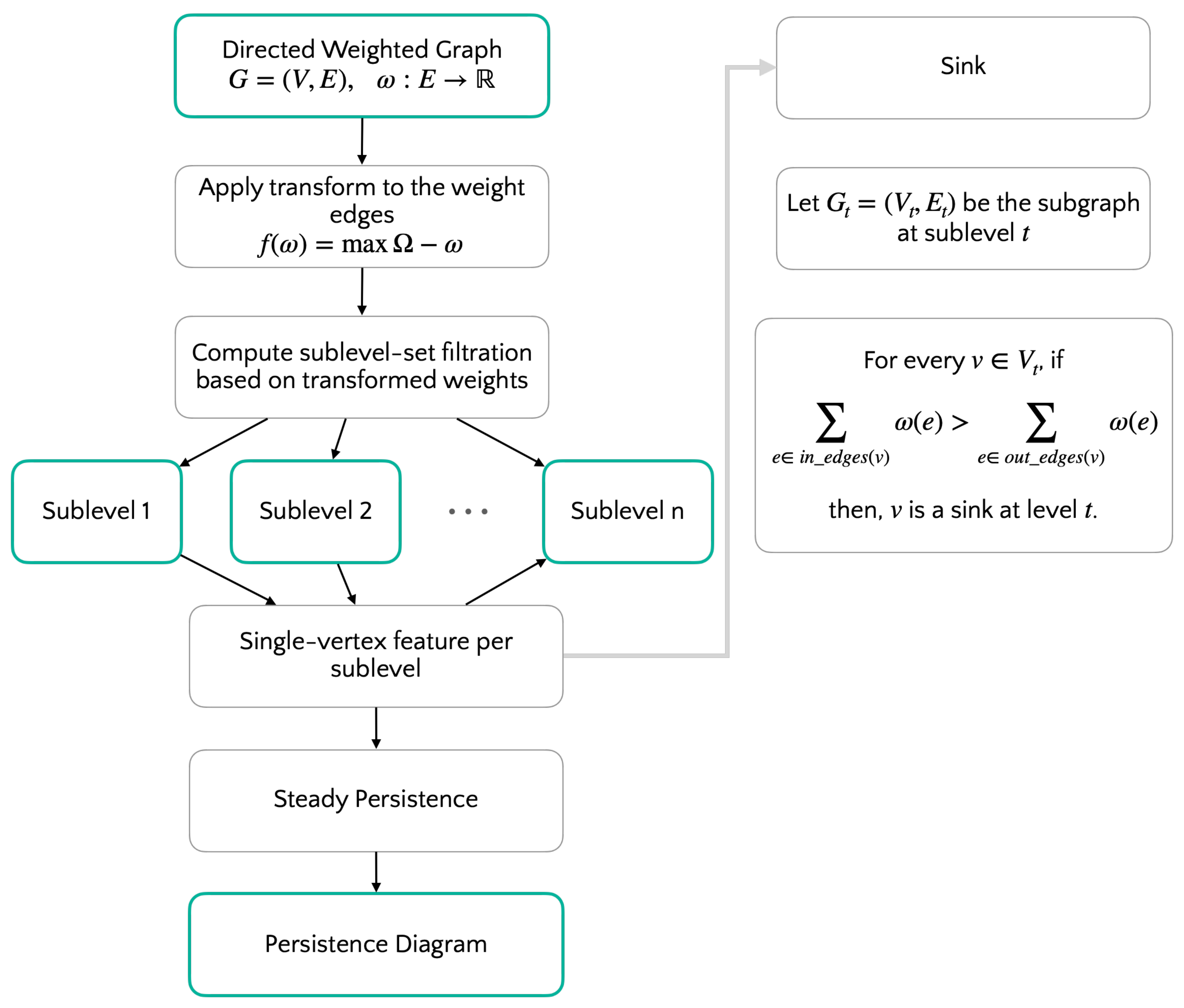
Figure 5.
Left. The persistence diagrams associated with the Bitcoin Alpha (top) and OTC (bottom) networks. Persistence diagrams represent the sink single-vertex feature. Histograms of the persistence values associated with trustworthy and fraudulent users are depicted in the right column. In each histogram, the black middle line is the median, while the white circle is the mean of the values.
Disclaimer/Publisher’s Note: The statements, opinions and data contained in all publications are solely those of the individual author(s) and contributor(s) and not of MDPI and/or the editor(s). MDPI and/or the editor(s) disclaim responsibility for any injury to people or property resulting from any ideas, methods, instructions or products referred to in the content. |
© 2023 by the authors. Licensee MDPI, Basel, Switzerland. This article is an open access article distributed under the terms and conditions of the Creative Commons Attribution (CC BY) license (https://creativecommons.org/licenses/by/4.0/).
Copyright: This open access article is published under a Creative Commons CC BY 4.0 license, which permit the free download, distribution, and reuse, provided that the author and preprint are cited in any reuse.


