Machine Learning-Based Forest Classification and Regression (FCR) for Spatial Prediction of Liver Fluke (<em>Opisthorchis viverrini</em>) Infection in Small Sub Watershed

Benjamabhorn Pumhirunroj; Patiwat Littidej; Thidarut Boonmars; Kanokwan Bootyothee; Atchara Artchayasawat; Attasit Wongkalasin; Eksakol Lertsiriudom; Phusit Khamphilung; Donald Slack

doi:10.20944/preprints202308.2039.v1

Preprint

Article

Machine Learning-Based Forest Classification and Regression (FCR) for Spatial Prediction of Liver Fluke (Opisthorchis viverrini) Infection in Small Sub Watershed

This version is not peer-reviewed.

Downloads

146

Views

Comments

Submitted:

28 August 2023

Posted:

30 August 2023

You are already at the latest version

A peer-reviewed article of this preprint also exists.

Abstract

Infection of liver flukes (Opisthorchis viverrini) is partly due to their suitability for habitats in sub-basin areas, which causes the intermediate host to remain in the watershed system in all seasons. Spatial monitoring of fluke infection at the small basin analysis scale is important because this can enable analysis at the level of the spatial factors involved and influencing infections. The spatial mathematical model was weighted by the nine spatial factors by dividing the analysis into two levels. 1) sub-basin boundary level analyzed with ordinary least square (OLS) model used to analyze spatial factors of liver fluke aimed at analyzing spatial factors related to human liver fluke infection according to sub-basin boundaries, and 2) infection risk positional analysis level with machine learning-based forest classification and regression (FCR) and displaying predictive results of infection risk locations along stream lines. The analysis results show 4 prototype models that import different independent variable factors. The results show that Model-1 and Model-2 give the most AUC = 0.964 and the variables that influence infection risk the most were distance to stream lines, and distance to water bodies, NDMI and NDVI factors rarely affect accuracy. This FCR machine learning application approach can be applied to the analysis of infection risk areas at the sub-basin level, but independent variables must be screened with a preliminary mathematical model weighted to the spatial units in order to obtain the most accurate predictions.

Keywords:

Opisthorchis viverrini

;

Forest-based classification and regression

;

Machine learning

;

Ordinary least square

Subject:

Environmental and Earth Sciences - Geography

1. Introduction

Severe liver fluke infections have been detected in Ponna Kaeo district, Sakon Nakhon province, Thailand [1]. The liver fluke, scientifically named Opisthorchis viverrini, causes cholangiocarcinoma (CCA) [2,3,4]. The prevalence of liver flukes and bile duct cancer cases have been reported to be the highest in Thailand, according to causes of liver fluke infection [5]. It is caused by eating raw fish contaminated with contagious larvae, as well as the popular consumption of raw or semi-cooked and semi-raw fish. Fluke infections from fish products such as fermented fish have also been reported [6]. Every year, more than 1,000 new cases of CCA are identified in Sakon Nakhon Hospital. This incidence has not decreased over the past decade despite the fact that the major risk factors for O. viverrini infection are known [7,8]. Another study reported that the incidence of CCA in four major regions of Thailand (Sakon Nakhon, Phrae, Roi-Et, and Nong Bua Lamphu) has not been identified [8,9,10,11]. Those with high severity of O. viverrini infection (>6000 eggs/g. feces) were 14.1 times more likely (odds) to develop CCA than people who were not infected [12]. The proportion of humans who have been infected with O. viverrini that has developed into CCA is about 10%, causing serious health emergencies throughout the region [13,14]. The O. viverrini infection can produce bile duct, liver, and connective tissue inflammation, resulting in the development of CCA [4,15]. The five-year survival rate of intrahepatic, distal extrahepatic, and hilar CCA patients undergoing surgery was 22–44%, 27–37%, and 11–41%, respectively [15].

Due to the geographical features of the area, there is a subdistrict boundary with the largest natural water contact zone in the northeast, namely Nong Han. The physical nature of the swamp is a large natural water source, full of water throughout the year, as it is a waterfront source from several streams, making it an important food source for the community. The livelihood of people living in the watershed derives from finding fish, which is an important source of protein, and there is a consumption culture that is familiar with the taste of raw fish [1,4], fascinated by the sweet taste of fresh, sour, spicy, hot fish with herbs cooked in meals. Fish is therefore a regular food for every meal of villagers who live near the river basin. According to preliminary screening results from 2019 to 2021 [2], a small number of people contracted liver fluke. In addition, studies conducted on the prevalence of liver fluke infection in fish (contagious larvae) showed that Sakon Nakhon province had an infection area of 33.33% [13], and a 2016–2017 study of the density of contact larvae in fish showed a density of 10–20 metacircaria per kilogram of fish [12]. As a result, liver fluke outbreaks are still present in Sakon Nakhon province, where the liver fluke's eggs are transfused with feces, potentially contaminating soil, water bodies, and causing recurrent infections and an endless cycle of infection.

The application of geographic information system (GIS) knowledge as an analytical tool is particularly useful because of the spatial analysis of liver fluke infections with remote sensing information systems. Remote sensing (RS) obtained from satellite imagery can provide in-depth analysis of the likelihood of liver flukes and their distribution [14], such as the standardized vegetation index, soil moisture index, soil cover index [16], and other indices that may be associated with the habitation of liver fluke intermediates. Many studies have applied spatial statistics to analyze spatial correlation factors to liver fluke infection [17], such as studies [18,19] that analyzed a large area, resulting in discrepancies and incoherence in raster data. Based on the findings of [20,21,22], GWR (geographic weighted regression) models were constructed in small area unit systems in hydrological factor analysis, resulting in high R² values in all other models. However, in this study, the OLS (ordinary least square) model was applied, which is a global operation model, which is sufficient to create a model to analyze areas with a small number of spatial units. Because GWR models require large enough units of space to be weighted by coefficients, OLS models are a satisfying alternative for small-space solutions.

However, since there are many indices that are to be constructed as independent variables, in order to accurately analyze them, the principles of geo-statistics [23], the OLS modeling method of local operations in particular, requires the creation of sub-spatial units [20], such as sub-basins, defined from the flow boundary of the sub-basin to the modeling control boundary. This makes OLS models effective in predicting and analyzing spatial relationships well [24]. To build spatial models for analyzing relationships in small areas such as sub-basin levels [25], there is a need to use appropriate models and design sub-area units to suit the distribution of data and dependent and independent variables. The application of only OLS models in independent multivariate analysis often provides satisfy accuracy, since there are many independent factors that create a lot of variability for the model. However, in this study, OLS modeling was used to analyze the relationship between a set of independent variables and the percentage of infections before OV. Past research on spatial modeling has not used the application of OLS models and sub-spatial unit boundaries in small watershed systems to track liver fluke infections. This is performed to screen for independent variables that are involved in spatial infections, and then OLS modeling is carried out, which can be accurately modeled using a small set of independent variables that are related to actual variables. To predict areas at risk of fluke infection spatially, it is necessary to develop models with the accuracy of predictive prototypes. Using forecasts from spatial statistical models, risk analysis can only be done at the sub-basin level, which requires sufficient independent variable data to create appropriate trendlines. Machine learning (ML) is therefore necessary and is used to predict the risk of water source location with potential infection by learning from spatial factors.

Modern research has applied ML to spatial risk assessment tasks such as [26].In recent years, advances in ML algorithms, computing power, and geospatial innovations including software have made it easier to create spatial maps [27]. The precision of spatial maps can be improved using machine learning algorithms. Knowledge-based methods [28], multivariate logistic regression methods [29,30,31] and multivariate binary logistic regression [32] have all been presented in recent papers. General linear model [33,34], quadratic discriminant analysis [33,35], boosted regression tree [34,36], random forest classification (RFC) [37,38,39,40], multivariate adaptive regression splines [41,42], classification and regression tree [34,43], support vector machine [44,45,46], naïve Bayes [47,48], generalized additive model [33,43], neuro-fuzzy and adaptive neuro-fuzzy inference [49,50,51], fuzzy logic [52], artificial neural networks [53,54,55,56,57,58], maximum entropy [59,60] and decision tree [31,61,62]. ML applications was also widely used to create landslide maps (LSM). Merghadi et al. [63] assessed the performance and competency of various ML techniques in the literature and discovered that tree-based ensemble optimization algorithms outcompete other ML algorithms. In a comparison analysis, Sahin [64] found that CatBoost had the best precision (85%), followed by XGBoost (83.36%) since the proportion of samples of the model was determined by Catboost was more precisely anticipated than other models. The primary advantages of ML and probabilistic processes are their objective statistical foundation, repeatability, capacity to quantitatively analyze the effect of variables on spatial prediction, and capacity to update them regularly.

Several studies in ML applications have shown that the random forest classificationmethod always has a higher receiver operating characteristic (ROC) and area under the ROC curve (AUC) effect than other models, but it also depends on the factors that bring the machine to learning, including the number of learning and testing points. Machine learning models can be built using a variety of spatial conditioning factors (land use, slope, aspect, elevation, road network, water body, factors from proximity etc.). Several studies on flood prone, landslide susceptibility, land use change evaluation have been undertaken using remote sensing and GIS techniques [65,66,67].

In this research, the Forest-based Classification and Regression (FCR) approaches were applied to predict the percentage of infection risk with spatial factors at both the watershed level and the location of learning points that are the locations of water bodies with infected fish. Therefore, if it can be demonstrated that the spatial characteristics in the distribution of each parasite are important to any subspace unit at the sub-basin level, then the sub-basin level can be properly managed for protection [68]. For example, breaking the cycle of intermediary hosts such as mollusks can prevent future illnesses and result in healthy communities. The community is strengthened, and the burden of medical care can be reduced.

2. Materials and Methods

2.1. The Study Area

Phon Na Kaeo is a district in Sakon Nakhon province; in the north, it borders Kusumal district; in the east, it borders Pla Pak district (Nakhon Phanom province); in the south, it borders Wangyang district (Nakhon Phanom province), Khok Si Suphan district, and Mueang Sakon Nakhon district; and in the west, it borders Mueang Sakon Nakhon district. Its geographical coordinates are 17^o13’18’’N, 104^o17’24’’E, as shown in Figure 1.

There are 5 subdistricts: Ban Phon, Na Kaeo, Nadong Wattana, Ban Khae, and Chiang Shi. The Phon Na Kaeo district’s area of Sakon Nakhon province is located in the east of the Songkram watershed, adjacent to Nakhon Phanom province and adjacent to Nong Harn marsh, which is a large natural water source. There is an exchange of Mekong fish and fish habitat in the area at a distance of about 40 kilometers from the Mekong River, resulting in the travel of many Mekong/tributary fish in the Phon Na Kaeo district, and the potential for fish to increase the number of liver fluke infections.

2.2. Datasets and Analyses

Liver fluke and cholangiocarcinoma have long been a public health problem in Thailand, and at present, at least 20,000 people in the northeast die from cholangiocarcinoma each year [69,70]. Currently, there are 6–8 million people infected with liver fluke, so screening people for liver fluke infection to eradicate the parasites is very important to reduce the risk of cholangiocarcinoma [71].

The data on people infected with liver fluke in this research were obtained from the Sakon Nakhon Provincial Public Health Office (SKKO) [72] https://skko.moph.go.th/dward/web/index.php?module=skko. Stool examination is a standard screening method that has been in practice for a long time. For example, intensive examination of parasite eggs in feces using the modified Kato–Katz technique, which has been an effective method in the past when there were prevalent parasite outbreaks. Moreover, stool examination is a standard method that has been in practice for a long time. Stool specimens were examined for O. viverrini eggs within hours of collection using the modified Kato–Katz technique [73]. The result of infection showed that most people were infected in Phon Na Kaeo district, Sakon Nakhon province. In the range of 18–80 years, the prevalence of infection tends to increase. Other testing methods include the FECT (formalin-ethyl acetate concentration technique) and the enzyme-linked immunosorbent assay (ELISA) [74], which are more effective than stool testing. It also provides quantitative results that correlate with the density of the parasite and can be used for post-drug assessment to determine the rate of reinfection or new infection [68,73,74]. However, in this study, such methods were not used, since they require a high budget. However, the secondary data obtained from SKKO of the number of people infected with liver fluke measured using the modified Kato–Katz method is reliable because it is an appropriate method for measuring many people.

The data on modified Kato–Katz fluke infection showed that most people were infected in Phon Na Kaeo district, Sakon Nakhon province. In the range of 30–40 years, the prevalence of infection tended to increase. As for the density of infection in patients, it was found to be similar to the prevalence, i.e., the density of liver fluke infection was highest among those infected in the province. Sakon Nakhon has a range of 20–30 years old, as shown in Table 1.

In 2019–2021, 12,063 cases were detected at the national level of stool testing and fell to the 8^th Health District Office (Region, (R8)) [75] https://r8way.moph.go.th/r8way/index. Of the 2,832 cases, 599 were found in Sakon Nakhon province, with the highest number of liver fluke infections in neighboring provinces in the interconnected river basin system Nakhon Phanom and Bueng Kan [76]. The summary of reported cases detected as a percentage is shown in Figure 2. Sakon Nakhon province has the largest freshwater supply in the northeast and is a water source that breeds animals during the rainy season [2]. Phon Na Kaeo has the highest average infection rate in Sakon Nakhon province, which is why the provincial health authorities must keep an eye on the situation. In this study, data on the number of people infected with liver fluke in Phon Na Kaeo district were used. The distribution of the percentage of infected persons to the population density is shown in Figure 3(a) and shows the percentage of infected persons according to the sub-basin boundary, where the percentage index of infections in 2019–2021 is 0.510–9.180 percent, which is developed as a dependent variable in the OLS model and linked to other independent data layers by means of geographic information system, namely the spatial join method, as shown in Figure 3(b).

The acquisition of Sentinel-2 satellite imagery data can be downloaded from Google Earth Engine (GEE) by coding the following settings: 1) Define the boundaries of Thailand with an area of interest, AOI 2) To set the download time period to '2019-12-01', '2021-01-31'. 3) Filtering removes only images with a cloud cover percentage of less than 10 percent 4) To combine the wavelength of Sentinel-2 image for visualization 5) Download the resulting image and calculate the remote sensing index. Details of coding are shown as follows:

//1) AOI for download Sentinel 2

var c = ee.FeatureCollection('USDOS/LSIB_SIMPLE/2017')

.filter(ee.Filter.eq('country_na', 'Thailand'));

//2) Load Sentinel 2 data

var image = ee.ImageCollection('COPERNICUS/S2_SR')

.filterDate('2019-12-01', '2021-01-31')

//3) Filter to 10 percent cloud cover

.filter(ee.Filter.lt('CLOUDY_PIXEL_PERCENTAGE', 10))

.filterBounds(c)

.median();

// 4) Band composite

var visParamsTrue = {bands: ['B2', 'B3', 'B4'], min: 0, max: 2500, gamma: 2};

Map.addLayer(image.clip(c), visParamsTrue, "Sentinel-2 Jan 2022");

// Applies scaling factors.

function applyScaleFactors(image) {

var opticalBands = image.select('SR_B.').multiply(0.0000275).add(-0.2);

var thermalBands = image.select('ST_*.*').multiply(0.00341802).add(149.0);

return image.addBands(opticalBands, null, true)

.addBands(thermalBands, null, true);

}

var dataset = applyScaleFactors(c);

var visualization = {

bands: ['SR_B4', 'SR_B3', 'SR_B2'],

min: 0.0,

max: 0.25,

};

2.3. Independent variable modeling

The independent variable set consists of 9 factors, namely X₁(index of land use types), X₂(index of soil drainage properties), X₃(the distance index from the road network , X₄(distance index from surface water sources), X₅(distance index from the flow) accumulation lines), X₆(index of average surface temperature), X₇(average surface moisture index), X₈(average normalize difference vegetation index), and X₉(average soil-adjusted vegetation index). Each factor is calculated to determine the average division per sub-basin area, and in addition, factors 6 to 9 calculated from the remote sensing index using raster calculator function are the average of the Sentinel-2 image range from January to April of 2019–2021, which is a picture of the dry season, allowing for analysis of the area where the host medium survives whilst waiting for the rainy season to arrive. Mathematical models have evolved from fundamental factors based on a variety of research related to variables influencing liver fluke infection in watershed level areas. as shown in the mathematical model for calculating each factor as Equations (1) to (12) as follows:

X_{1} = \frac{{W L}_{j} L_{j}}{A_{k}}

(1)

where

X_{1}

is index of land use types suitable for intermediary host housing.

{W L}_{j}

= any type i land use weight value where i = (1 = built-up), (2 = forest), (3 = miscellaneous), (4 = paddy field), (5 = rice paddies in irrigated areas and water body).

L_{j}

= area of land use category j unit (sq.m.).

A_{K}

= size of sub-basin area at any k unit (sq.m.). Adapted from the research of [12].

X_{2} = \frac{W_{j} S_{j}}{A_{k}}

(2)

where

X_{2}

is the index of soil drainage properties suitable for the habitation of the intermediate host.

S_{j}

= area size of drainage properties of any type j soil.

W_{j}

= weight value of drainage of any type j soil. Adapted from the research of [7].

X_{3} = \frac{\sum_{i = 1}^{n} \sum_{j = 1}^{m} {D R}_{i} B_{j}}{A_{k}}

(3)

where

X_{3}

is the distance index from the road network used to analyze the suitability of the intermediary host from water trapped by the road network.

{D R}_{i}

is the distance from the road line out to any distance K (meters), where k starts from 500 m, 1,000 m, 1,500 m, 2,000 m, and more.

B_{j}

is the buffer distance at any k distance where K starts from 500 m, 1,000 m, 1,500 m, 2,000 m, and over. Adapted from the research of [16].

X_{4} = \frac{\sum_{i = 1}^{n} \sum_{j = 1}^{m} {D W}_{i} B_{j}}{A_{k}}

(4)

where

X_{4}

is the distance index from surface water sources used to analyze the suitability of the medium host from embedding to the soil surface when moisture still accumulates in the dry season.

{D W}_{i}

is the distance from any surface water source i that goes out at any distance k, where k starts from 500 m, 1,000 m, 1,500 m, 2,000 m, and over. Adapted from the research of [6].

X_{5} = \frac{\sum_{i = 1}^{n} \sum_{j = 1}^{m} {D S}_{i} B_{j}}{A_{k}}

(5)

where

X_{5}

is the distance index from the stream lines or accumulated flow lines of water used to analyze the suitability of the medium host regarding waterlogging and moisture accumulation in the dry season.

{D S}_{i}

is the distance from any of the accumulated flow lines of water at any distance k where k starts from 500 m, 1,000 m, 1,500 m, 2,000 m, and over. [20].

X_{6} = \frac{\sum_{i = 1}^{n} T_{i} A_{i k}}{A_{k}}

(6)

where

X_{6}

is the index of average surface temperature in any sub-basin used to analyze the suitability of the medium host from subsurface embedding to sub-basin.

T_{i}

any grid temperature value in degrees Celsius.

A_{i k}

is the total area of temperature at i degrees Celsius within the sub-basin boundary at k. Adapted from the research of [9].

X_{7} = \frac{\sum_{i = 1}^{n} {N D M I}_{i} A_{i k}}{A_{k}}

(7)

where

X_{7}

is the average surface moisture index in any sub-basin used to analyze the suitability of host media from subsurface embedding in the sub-basin.

{N D M I}_{i}

is any grid surface moisture value.

A_{i k}

is the total area of surface moisture at i that is within the sub-basin boundary at k. Adapted from the research of [18]. Waterbody distribution: As water availability boosts the variety of species and natural resources, which helps extracting the location of areas where surface moisture can be maintained, clearly separated from the dry soil surface using the Normalized Difference Moisture Index (NDMI) to emphasize it in a satellite picture that was chosen. NDMI ranges from -1 to 1, with water bodies usually having NDMI values greater than 0.4 In the distribution classification of waterbodies, NDMI values were divided into five groups, with higher values indicating the high likelihood of intermediary host habitat. The following equation was used to determine the NDMI of the study area using

N D M I = \frac{G R E E N - S W I R}{N G R E E N - S W I R}

(8)

X_{8} = \frac{\sum_{i = 1}^{n} {N D V I}_{i} A_{i k}}{A_{k}}

(9)

where

X_{8}

is the average vegetation index in any sub-basin used to analyze the suitability of the medium host from subsurface embedding to sub-basin.

{N D V I}_{i}

is any grid-normalized difference vegetation index.

A_{i k}

is the total area of vegetation index at i within the sub-basin boundary at k. Adapted from the research of [18].

Twelfth sets of satellite images were downloaded from Sentinel-2. The following equation was used to determine the NDVI of the study area in ArcGIS pro v.2.9.0 under map algebra function as follows.

N D V I = \frac{N I R - R E D}{N I R + R E D}

(10)

For Sentinel-2, NIR represents the near-infrared band 8 (0.842–0.865 µm) and RED the corresponding band 4 (0.665–0.704 µm). NDVI values are straightforward visual indicators that may be used to examine remotely sensed data and determine if there is living, green vegetation present [12]. The NDVI ranges from −1.0 to +1.0, a positive value indicating dense and healthy vegetation. The research identified five unique vegetation distribution groups based on NDVI values, with greater values indicating a region with a suitable potential of host intermediaries.

X_{9} = \frac{\sum_{i = 1}^{n} {S A V I}_{i} A_{i k}}{A_{k}}

(11)

where

X_{9}

is the vegetation index for adjusting the average soil in any sub-basin to analyze the suitability of the medium host from subsurface embedding in the sub-basin.

{S A V I}_{i}

is the i-any grid soil adjusted vegetation index value.

A_{i k}

is the total area of soil-adjusted vegetation index at i within the sub-basin boundary at k. Adapted from the research of [19]. Soil-Adjusted Vegetation Index (SAVI), the vegetation index created for the calculation of vegetation in the study area with relatively low vegetation content has a similar calculation formula to NDVI, but a constant value (0.5) was provided for the Sentinel-2 image to reduce the influence of reflection from the lower ground soil of vegetation.

S A V I = \frac{N I R - R E D}{N I R + R E D + 0.5} x (1 + 0.5)

(12)

2.4. Ordinary Least Square (OLS) approach for spatial modeling (analysis at the level of infected in sub-basins)

Surface moisture factors and surface cover indicator indicators analyzed using satellite images are represented by calculations of independent variables from X₆ to X₉. An OLS modeling study was used for analyzing spatial correlations to liver fluke infection (OV) from remote sensing data of sub-basin-level prototype areas. The research algorithm is divided into 3 stages: 1) Data collection and manipulation to collect and manage data for use in analyzing the relationship of liver flukes to watershed areas in sub-basins. Starting with the preparation of Sentinel-2 satellite imagery data used in the study, January–April 2019, 2020, and 2021, the dry season of each year is when mollusks are embedded in moist soils waiting for rain to come during the rainy season. A total of 12 satellite imagery data (4 images per year, 3 years) were taken to average the image points and used to calculate the indices X₆, X₇, X₈, and X₉ for use as independent variables in the OLS model. 2) Independent variable screening and 3) alternative modeling. A detailed display of the steps can be shown as follows.

(1) Field surveys and OLS modeling for analyzing the relationship between liver flukes and spatial factors, including the NDVI, which is a value that indicates the proportion of vegetation covering the surface by taking the NIR and the red wave range reflected from the surface to calculate the reflection difference, making the NDVI value between -1 and 1 if the plant does not have green leaves, which returns a similar value of 0, while the value 0 means no vegetation if there is a density of plants with green leaves equal to 1. The other index group is the soil reflection value. In this study, the SAVI refers to the ratio between the difference between the amount of energy reflection during the near-infrared wave NIR and the amount of energy reflection in the red-light wave range to the sum of the amount of energy reflected during the NIR and the energy reflection coefficient of the soil, and the SAVI refers to the vegetation index calculated from two times the sum of the NIR plus one minus the square root. Taking the difference between doubling the NIR plus one all squared and eight times the NIR minus the total red wave divided by two, the two indices range from negative to maximum to 1, where the index values that are suitable for the habitation of the liver fluke medium host are approximately -0.2 to 0.2 of the SAVI indexes. The following is an explanation of the workflow of the OLS model, as shown in Figure 4.

(2) The OLS model uses the principle of estimating the coefficients of the equation with the same squared method as the conventional linear model, but the creation of a variable dataset is a geostatistical statistic that can generate a dataset from a smaller sample but retain a Z value that is similar to the original Z value. The area that seems to be the ideal area for shellfish implantation is the buffer area away from the accumulated flow line of water [20]. The variable data according to the data are generated as points of the village location where the OV data were surveyed; the independent variable group 1 (spatial variables) were represented as variable X₅ (distance index from the flow accumulation lines); the mean of the line length, the level 3 to 3 water flow level, is a variable that shows the likelihood of embedding the host's intermediary of liver flukes along two sides of the stream by 500-2,000 meters. OLS creates a local regression equation for each feature in the dataset. When values for a cluster of spatial descriptive variables are available, problems with local multicollinearity are more likely. The conditional number (Cond) field in the output feature class indicates when the result is unstable due to local multicollinearity.

(3) OLS modeling the relationship between liver fluke, other types of parasites, and spatial factors uses a global model of spatial statistics, i.e., a model created specifically for each sub-basin, which allows for predicting liver fluke and other types of parasites and analyzing relationships.

The model serves to determine the coefficient of the relationship between the independent and dependent variables using the distance reciprocal weighting method, where OLS obtains a model to predict every unit area with a difference in coefficients [9,21,22]. OLS modeling must create a data layer based on this research, namely the percentage of liver fluke infection of the sub-basin region to be analyzed from 5-meters DEM data, the import of independent variables consisting of index variables generated from the wavelength correlation of satellite images in mathematical functions, and other spatial factors such as distance from water bodies and roads.

The OLS model uses sub-spatial statistics to find the relationship between independent and dependent variables and analyzes a polylinear regression equation to estimate the regression coefficient at each linear regression point or survey point, as shown in Equation (13) [25].

\begin{array}{l} y_{i} = & β_{0} + β_{1} (l a n d u s e) + β_{2} (s o i l) + β_{3} (r o a d) + \\ β_{4} (w a t e r b o d y) + β_{5} (s t r e a m l i n e s) + \\ β_{6} (s u r f a c e t e m p) + β_{7} (n d m i) + β_{8} (n d v i) + \\ β_{9} (s a v i) + [ε] \end{array}

(13)

where

y_{i} =

the value observed for the dependent variable at point i;

β_{0} =

the interception point y (constant value);

β_{n} =

the regression coefficient or slope of the explanatory variable n at point i;

x_{n} =

the value of the variable n at point i; The X variable can be described as: X₁ (index of land use types), X₂ (index of soil drainage properties), X₃ (the distance index from the road network, X₄ (distance index from surface water sources), X₅ (distance index from the stream lines or flow accumulation lines), X₆ (index of average surface temperature), X₇ (average surface moisture index), X₈ (average normalize difference vegetation index), and X₉ (average soil-adjusted vegetation index).

[ε] =

the error of the regression equation.

The expected outcome is a set of independent variables that illustrates the relationship between independent variables and dependent variables obtained using geographically weighted analysis of least square regression equations with the difference in independent variables affecting dependent variables in each sub-region (spatial nit). Therefore, if it is possible to analyze the spatial characteristics of the distribution of each type of parasite, the agency or organization can know the areas where the analysis results are used to correctly manage the parasite infection prevention system [77]. Preventing future illnesses can help communities stay healthy and reduce the burden of medical expenses.

2.5. Forest-Based Classification and Regression (Analysis at the location level of infected water bodies)

The principle of Random Forest is to create several models from the decision tree (from 10 models to more than 1,000 models), each model will receive a different data set, which is a subset of all data sets. When making a prediction, let each decision tree make a prediction of the data set and calculate the prediction result by voting output that is most selected by the decision tree (in case of classification) or find the mean value from the output of each decision tree (in case of regression). Each decision tree model in the random forest is considered weak learner, it is estimated that it is not very good model, but when each decision tree is used to make predictions together, it will get a total model that is more competent and accurate than the decision tree that makes a single prediction. The process of connecting OLS and machine learning is shown in Figure 5.

The Forest-based Classification and Regression (FCR) tool trains a model based on known values (Infected-OV points) provided as part of a training dataset. This prediction model can then be used to predict unknown values in a prediction dataset that has the same associated Independent variables. The tool creates models and generates predictions using an adaptation of Leo Breiman's random forest algorithm [78], which is a supervised machine learning method. The tool creates many decision trees, called an ensemble or a forest, that are used for prediction. Each tree generates its own prediction and is used as part of a voting scheme to make final predictions. The final predictions are not based on any single tree but rather on the entire forest. The use of the entire forest rather than an individual tree helps avoid overfitting the model to the training dataset, as does the use of both a random subset of the training data and a random subset of explanatory variables in each tree that constitutes the forest.

FCR is an effective decision tree ensemble used for large-scale and multivariate pattern recognition [79]. This ensemble learning is established based on the concept of the random subspace method [80] and the stochastic discrimination method of classification [81]. The RFC was then further extended by Breiman [82] who introduced the concept of bagging and random feature selection. Equipped with these features, a random forest model becomes a powerful tool to construct an ensemble of classification trees. Successfully applications of FCR have been reported in various studies [83,84,85], including landslide modeling [86,87].

Based on the FCR application of [61], the model is summarized as follows. Given a labeled data set (D) for training D = (X, Y), in which x_i ∈ X (i = 1,2, . . . , N, where N is the number of training samples) is a data sample and y_i ∈ Y is its class label, the FCR method aims at constructing a model, which is capable of separating the input space into different disjoint regions. Each of the regions is characterized by one class label. To achieve this goal, the method trains k individual decision trees, where each tree is associated with a random Θ_k vector, which represents a subspace of the original input space. Subsequently, a single tree k is constructed by sampling with replacement n < N data samples from the original training set. An individual tree (h_k) is therefore expressed as:

h_k (X, Θ_k) = Y

(14)

During the training phase of a decision tree, a node can be expanded with two children to enhance the data classification performance (see Figure 4). This process is characterized by a split cut at the corresponding dth dimension of the input data. The decision tree algorithm selects the most suitable node using the Gini impurity index (G) product (P) [83]; this product is computed as follows:

P = G₁G₂

(15)

where a Gini impurity index (G) of set k is defined as follows [88]:

G_{k} = 1 - \sum_{i = 1}^{n_{k c}} p_{k i}^{2}

(16)

where n_kc represents the number of classes in the considered set and p_ki denotes the ratio of the present class i in this set.

When a new input query is presented to the model, the RFC determines its output class through the majority vote standard [89]. Thus, the class label (y) of an input data x is computed from the established ensemble in the following manner:

y = H (x) = \frac{a r g m a x}{z} (\sum_{k} I {(h}_{k} (x, Θ_{k}) = z))

(17)

where I(t) denotes an indicator, function defined as follows:

I (t) = \{\begin{matrix} 1, t i s t r u e \\ 0, t i s f a l s e \end{matrix}

(18)

3. Results

3.1. Mapping of The Spatial OV Infection (Y, Dependent Variable)

Spatial subspace unit boundaries need to be created to define the amount of data. In this study, using digital elevation model (DEM) data with a cell size of 12.5 meters to generate sub-basin layer data, the results of the analysis were obtained from 10 sub-basin boundaries, sub-basins distributed according to the flow sequence level (3 to 6) from upstream to downstream at the marshes shown in Figure 6, and other descriptive information of the sub-basin, such as its size. The DEM dataset was readjusted for spatial height using the fill and sink function, which is a hydrological analysis method that uses GIS processes to process the altitude data as realistically as possible and enable continuous water flow analysis.

The highest spatial height mean was 180.397 meters at the river basin named Wanplachuem-1, followed by the Wanplachuem-2 and Phonkaeyai basins. They have values of 174.412 and 172.894 meters, respectively, with the upper basin of Phon Na Kaeo district being considered a basin of this height. However, even though it is in the upper basin, there is a high percentage of people infected with OV in these areas. Due to the multiple seasons, flooding causes surface water to flood up to the upper basin, making it possible for intermediate host mollusks and carp groups to move to feed in these areas.

Regarding the watershed with the highest risk of infection, when analyzed using DEM data, it was found that the Jomjaeng, Poopim, and Phonnoi basins had lower average height than other basins, and when looking at the percentage of infected persons, the percentage of infected persons was higher than 6.48 percent, as well as other species found in the river basin in this area, have a very high risk of having liver fluke eggs. The case percentage data shown as points is converted into raster data with a heat map command to use this raster data to find the average of the percentage infected and link it with other independent variable data using raster image, as shown in Figure 7. The display of the case percentage data shows the continuity of the number of infected people, so that the average calculation is equal for all sub-basins, but it will vary depending on the large and small values of the points used to calculate the raster. In this case, the Z value is the percentage of infected people in the village position. The radius of creating a raster map using a heatmap is from 2 km and 4 km so that raster data can be connected to all subtleties. The green areas show sparse percentages of infected people, and red areas show density and high chance of encountering infected people. The OLS model requires a continuity value of raster data, where the creation of heatmaps of infected people enables consistent analysis of positional data and other raster of independent variables and can generate trend graphs.

3.2. Mapping of The Independent Variables

The values of the indexes of the nine independent variables used to create mathematical models from Equations 1 to 9 are shown as descriptive data values, as shown the results of analysis in Figure 8. An important step in the GIS process used in the creation of multi-raster and vector, all methods of spatial data interpolation were used in the preparation of independent variable sets with ArcGIS pro v. 2.9.0. The percentage of cases was very high in the Wanplachuem-1, Phonnoi, and Wanplachuem-2 sub-basins, with values of 9.18, 7.84, and 6.489 respectively. The areas of the three watersheds are adjacent to each other and connected by an outlet. When observing the values of almost all indices of the river basin, Wanplachuem-2 is more valuable than other basins because the value of the index is divided by the size of the smaller basin area more than the other basins. Spatial units of the sub-basin with similar island index values of the X₁ index for Jomjaeng, Phonnoi, and Phonkaeyai are 14.773, 17.688, and 14.279, respectively. The island values of X₂ for Wanplachuem-2, Klangmai, and Nakaew are 24.128, 24.577, and 29.858, respectively. The island groups of X₃, X₄, and X₅ are in the same basin: Jomjaeng, Phonnoi, Phonkaeyai, Wanplachuem-1. The groups of remote-sensing indices are not very different, but they need to be analyzed together with other factors in OLS modeling and screened for duplication of factors again using correlation analysis. Different groups of factor index values require data standardization using mathematical models. Standardizing data to a comparable range allows OLS models to increase the accuracy of build and fit models better than using raw data directly to import models.

The results of the raster map data of the X₁ variant were distributed within a buffer distance of up to 500 meters, distributed over most areas of all sub-basins, and the results were similar to the X₃ index values, but there was a difference in the upper basin areas with low index values due to the lack of road networks. The X₄ and X₅ index map values showed high scores scattered mainly in the lower basin and low values scattered in the upper areas because the lower ones are close to large freshwater marshes. The X₆ index shows the distribution of the intermediate index mainly on the map, Figure 8(f) shows yellow with a flat surface temperature in the range of 26–28 degrees Celsius, while high-temperature areas are shown in red and are mostly structures such as road and village structures. The X₇index shows the distribution of high-level indices that are suitable habitat substrate host areas, mainly areas near water bodies with index values greater than 0.6 or more. The X₈ and X₉ indices are similarly distributed because they are made of vegetation index, but the X₉ index adds a constant value to make the vegetation value more reflective, both of which can be used interchangeably. To ensure modeling, consistency results can be observed from correlation, and the red area of both indices indicates that they are suitable areas similar to the X₇ index.

The results of the correlation of the independent variable mean calculated for each of the 10 watershed units showed that the pareto plot could show different correlation values and preliminary correlation trends could be observed. The variable factor based on the average of infection percentages showed that the area with the average infection rate Y(% of OV) differed from other basin areas as many as 5 basins by observing the curve intersecting the Y-axis at 80 percent, namely basin areas Maikrabok, Klangmai, Wanplachuem-1 and 2, and Phonnoi, respectively of mean difference, as shown in Figure 9(a). Pareto graphs showing correlation screening over a similar number of river basins include the X₁, X₂, X₃, X₄ and X₅ variable analysis graphs that have similar trend curves and culled the river basins that found significant correlations in the range of 5 to 6 river basins, as shown in Figure 9(b)-(h). The pareto graph of the correlation analysis of factors calculated from most remote sensing indices can screen areas on a scale of 2-3 watersheds that still have a significant correlation of the index mean, with the highest screen able factors being X₅, X₆, X₈ and X₇, respectively as shown in Figure 9(g)-(j). However, this correlation analysis shows that in many sub-basins, each factor has shown a significant correlation, which makes it possible to formulate a hypothesis that each factor can be modeled in the analysis of coefficients related to infection. This analysis is based on the average of factors divided by the watershed, resulting in large-scale analysis, but infection prediction targets focus on predicting the location of risk areas, so the number of independent variables and the maximum associations associated with infection must be considered for further introduction into machine learning on FCR.

3.3. Spatial Analysis of Factors Associated with Spatial Liver Fluke (Opisthorchis viverrini) Infection

Independent variable redundancy needs to be reduced in the number of variables so that OLS models can still create models that maintain R² values at acceptable levels [90]. Spatial correlation analysis was the method used to screen for independent variables [91] in this study. The group of independent variables is classified into two groups: variables generated from vector data solving factors X₁ to X₅, which are characterized by points, polylines, and polygons. Importing this type of datum that is analyzed together with other variables does not require first generating raster data and assigning score values to different data ranges to measurable standards. The factors X₆ to X₉ are already raster data, but they were calculated in the form of mathematical models to standardize the data so that they could be correlated with the previous set of variables. Table 2 shows that factors X₃ to X₅ are negatively correlated with the percentage of people infected with OV, which suggests that the longer the distance away from that set of factors, the lower the chance of catching the fluke, but in contrast, the closer the distance is, the greater the risk of infection if fish is consumed within the nearby radius. Factors X₁ and X₂ show that the poorer the drainage, the greater the risk of infection because the soil can retain moisture better than well-drained soil, and the more agricultural and agricultural land use near irrigation canals, the more moisture the soil surface has to use than other types of land. When analyzing the correlation of vector factors, factor X₅ can represent factors X₁ to X₄ because it correlates with the percentage of infected people -0.226. The factors X₁ and X₄ are 0.985, 0.838, 0.984, and 0.612, respectively.

In addition to screening the variables that were used to create the OLS model, namely the set of independent variables X₅ to X₉, this set of variables was used to create correlation graphs to analyze the regression of the model. To determine the properties of regression patterns, two methods of residual plot graph analysis were used. The first is residual plots, which is a plot of values. Residuals are estimates of Y (% of OV)-fitted values, and should be randomly distributed when observations occur. The second method is to plot the normal probability plots of the error coupled with the expected value. If the plot is shaped close to a straight line, the discrepancy has a normal distribution. The X₅ variable set demonstrates the normal distribution of data compared to the variables according to the section. The variables X₆ to X₉ have a vertical distribution of the dataset, which translates into a narrow range of index values that can predict the percentage of infections over a wide range, as shown in Figure 10.

3.4. Optimal OLS Model for Predicted with Liver Fluke (Opisthorchis viverrini) Infection (Watershed level)

Comparing multiple alternative models increases the chance of selecting the right model to predict [92,93]. Spatial factor correlation simulation is the use of an independent group of variables as an alternative to OLS modeling to visualize trends of tolerances at the small area unit level. The set of independent variables imported into models were selected using correlation analysis, and the variables X₅ to X₉ were selected, simulated, and displayed, as shown in Table 3. An appropriate OLS model to predict the percentage of infected people can be observed from the analysis results; R² is high. The variable is significant at a high level (i.e., t-statistics are very high or p-value is very low) [94,95]. The results of the models in the table compared the precision between 4 models to visualize the difference in the accuracy of the models [96].

The alternative model proposes four alternative models: Y(%OV1), Y(%OV2), Y(%OV3), and Y(%OV4), as shown in Table 3. The results of OLS model 1 Y(%OV1) imported two independent variables, X_8ndvi and X_9savi, to test whether they were expected to be negative per percentage of infected people. Results of spatial non-stationarity [18,20], and R² values are compared to OLS models. The model shows negative coefficients on the scales of -1.534 and -6.032, respectively, and t-stat values of -0.878 and -2.212, and p-values of 0.226 and 0.125, indicating that both factors have not yet correlated significantly with the percentage of infected people. Additionally, the model displays the R² value of the OLS model that is higher than the 0.524. Both factors show an acceptable level of relationship with R² and therefore need to be tested in the second alternative model.

The 2^nd OLS model Y(%OV2) shows the correlation coefficient of factors X₇(ndmi) positively, but the X₈(ndvi) and X₉(savi) factor begins to show negative results indicating that the more areas of separation between vegetation covers, the lower the percentage of infected people. The X₉(savi) factor showed statistical significance with a t-stat (-2.326) greater than the other two factors and a p-value (0.038) of less than 0.05, which made it possible to find a tendency that the mid-range and less-than-peak soil correction index factors increased the chance of a percentage of people infected with liver fluke. Alternative models 3 and 4 incorporated the X₅(stream) factor into the model, resulting in an increase in R² accuracy to 0.713 and 0.681. The coefficients of X₅(stream), X₇(ndmi) and X₈(ndvi) reveal a t-stat and p-value that are more significant than other variables and show a negative trend together. An optimal OLS model for predicting case percentage was model 3 Y(%OV3) because it can provide a confidence level greater than 71.3 % and there are still not too many independent variables that can cause prediction results to be inaccurate even if model 4 Y(%OV4) has a higher R² value than model 1 Y(%OV1) and model 2 Y(%OV2), but it may cause duplication of the independent variable set and coincidence resulting in higher R² trade.

The standard residual index (SR) was used to determine the prediction accuracy of a model as an index used to verify the accuracy of a model by displaying the standard value in intervals of 0.5 [20,25], as shown in Figure 11. Sub-basin units with SR values ranging from -0.5 to 0.5 are sub-basin areas where OLS models can predict accurately and have lower tolerances than other areas. Sub-basins Maikrabok, Nongphue, Nakaew, and Klangmai that show the range of -0.5 to 0.5 are shown in yellow in OLS model3 and have a tolerance 3 units lower than OLS models. It is also confirmed by the SR results obtained from OLS model 3 Y(%OV3) and model 4 Y(%OV4) that the deviation area has the same direction and can reduce the number of units of the discrepancy area even more, namely the sub-basin areas named Wanplachuem-1 and Phonkaeyai, respectively. The results of this SR index analysis were used to design a policy for reducing the suitability of embedding the medium host in moist soils.

3.5. Spatial prediction of OV-Infection using Forest-based Classification and Regression (FCR) (Location level)

The location of the water bodies where these fish infected with liver fluke was found was used as a set of points for machine learning, which is the boundary location of the banks of water bodies. This section presents the experimental results of the FCR model used for predicting spatial fluke infection. Sensitivity mapping, as previously stated, to train and test the ability to predict the original model. Datasets were randomly divided into training (60%) and testing (40%) sets. In all data sets, training and testing. The sets are 35, 21 and 14 respectively as shown in Figure 12.

In addition, to reduce the bias caused by sampling in the data sampling process, repeated sampling is performed with 10 runs, including the learning setting is number of trees = 100, leaf size = 5, tree depth range = 1-5. The experimental results of the proposed FCR model are reported in Tables 4 to 6. Forecasting model integration uses a boosting method, with the principle that multiple data classification models are created. Each model uses the same set of train data to build it, each of which has an additional weighted value. Weighted voting methods were used and new data groups were assigned with the highest number of votes (majority voting), which in this study used two methods: average and weighted.

The FCR model from this study provides a method that makes decisions for each model independent of each other using the same algorithm but allows each instance to learn from different payloads using random selection. This mechanism was called bagging and pasting, the difference is that bagging can randomly select the same item, but Pasting does not allow duplicates to be randomized at all. This results in more stable models and often more accurate than pasting.

The model out of bag errors is shown in Table 4. The set of independent variables that were introduced to FCR's machine learning was used in all four factors based on the selection results of the OLS model with the highest R² value of 0.713: distance to streams, distance to water bodies, NDMI, and NDVI. The distance factor from the water resource was also included in the simulation because the importance of similar factors of the water source was known. The results showed that the number of cycles increased from 50 to 100 of number of trees in all MSE tests showed a decrease in every set of independent variables by the distance to streams factor from 10.203 to 8.98, which equates to the addition of a set of 4 independent variables and % of variation explained between -46.689 and -29.111. When considering the importance of each variable, it was found that the order of weight values in distance to water, distance to stream lines, NDVI, and NDMI showed importance of 23.18, 39.7, 20.32, and 22.79 percent, or 37%, 22, 22, and 19%, respectively, as shown in Table 5. The FCR model uses ArcGIS pro v.2.9.0 software package for analysis under forest-based classification and regression functions.

Machine learning-based FCR simulation was made into 4 models as shown in Table 6, which describes the synthesis of ranges of independent variables, found that the degree of overlap between the range of training data and the input explanatory variables of Model-1 has a share value of 1 and a test value of 0.45. The percentage of overlap between the range of monitoring data and training data ranges from 0.00 to 0.45. This data shows that the location of the learning point can be the test point for the accuracy of the FCR model. Model-1 uses independent variables as distance to stream lines, Model-2 uses independent variables as distance to stream lines and distance to water bodies, Model-3 uses independent variables as distance to stream lines and distance to water bodies, and NDMI, and Model-3 uses independent variables as distance to stream lines and distance to water bodies, NDMI, and NDVI, respectively, which are used to simulate spatial distribution of infection. The training range of the Model-1 ranges from 0.48 meters to 1055.51 meters, while the validation ranges from 133.04 meters to 610.29 meters. The training share value can be used together in all the same ways as for example Model-2 and Model-3, while Model-4 has only a secondary factor that can use overlapping learning points.

3.6. Spatial Prediction of OV-infected

The results of the machine learning data set and regression synthesis when only one independent factor with a high priority weight of distance to stream lines were imported with an R² value of 0.775, and when the other three factors were imported, the R² values were 0.853, 0.859, and 0.849 respectively. The standard error of the Model-3 is the minimum of 0.043 and the highest is the Model-2, but it is considered not far apart significantly. When observing the preliminary statistics, it is evident that there is no difference between Model-2 and Model-4, but from the observation of the Model-1 model, only one variable of learning is imported but also provides a satisfactory level of accuracy statistics, indicating that distance to stream lines affect machine learning.

Therefore, it was necessary to show all four models to see the trend of change in the percentage of liver fluke infection. This was to provide spatial confirmation of how the location of infection risk in all four models can confirm location and severity. The location used to predict infection is a point simulation based on the location of the fishing area of the villagers who regularly use it obtained from the inquiry. These locations are linked to the spatial resolution data of the 10-meter point Sentinel-2 satellite imagery.

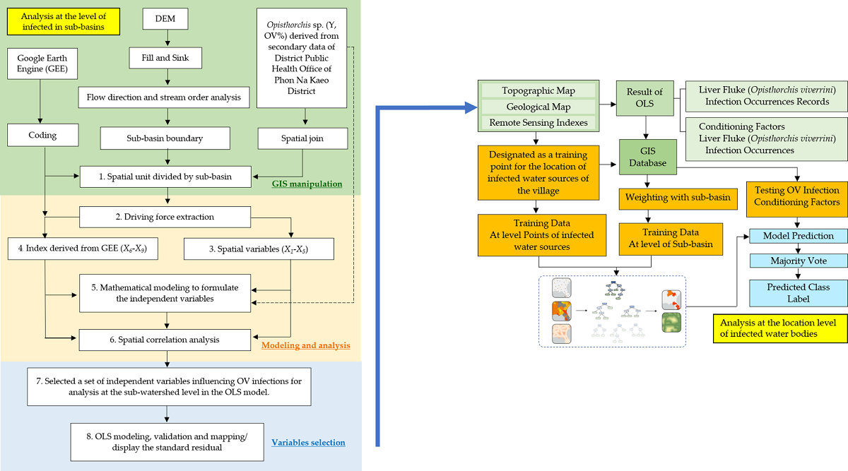
The receiver operating characteristic curve (ROC curve) was a popular method used to measure the accuracy of forecasts. The ROC curve was a graph with a correlation between the y-axis instead of sensitivity (true positive rate) and the x-axis instead of 1-specificity (false positive rate), as shown in Figure 13. As shown in Figure 13(a) to (e), or the area under the ROC curve, the ROC curve indicates the validity or reliability of the prediction model if any prediction model has the most space below the AUC (ROC curve) is considered the most effective.

Table 7. The training data: regression diagnostics.

Training Data: Regression Diagnostics	Model-1	Model-2	Model-3	Model-4
R-Squared	0.775	0.853	0.859	0.849
p-value	0	0	0	0
Standard Error	0.053	0.06	0.043	0.051

*Predictions for the data used to train the model compared to the observed categories for those features.

Figure 13. Display receiver operating characteristic (ROC curve) and AUC: area under the ROC curve compare 4 models: (a) model-1, (b) model-2, (c) model-3, (d) model-4, and (e) all model.

Results of Models-1 and 2 of FCR using resampling techniques could accurately predict the percentage of infected fish at an accuracy range of 0.775 to 0.859 from Figure 13(a) and (b). display ROC, which is a popular method used to measure the accuracy performance of forecasts. Models-1 and 2 of FCR could predict the severity of the percentage of infected fish with the result of an area value under the ROC curve of 0.964, both the highest of all prediction models. False positive rate below 10 percent and true positive rate above 90% also use a smaller number of model coaching data. This makes the time of training of models predicting the severity of the percentage of infected fish take less time, but nonetheless the effect of space under the graph. The ROC curve of models 3 and 4 is also very high and could be used as a prediction model as well.

The final forecast was a positional simulation of villagers' fishing sites along the tributary streams that flow into the sub-basin within the boundaries of the district. The total number of positions used to simulate the forecast is 103 points as shown in Figure 14. It was a location used by locals and fishermen in the area to go fishing for consumption. These positions, obtained through field inquiries and inspections, were located within 30 meters of the stream lines layer and water bodies.

The FCR simulation results of each model were shown in Figure 14, with Figure 14(a) showing the simulation of the chance of infection of Model-1 ranging from 2.027 to 6.222. The range with the highest percentage of infections ranges from more than 5%, with 10 points showing distribution in the sub-basins of Phonnoi, Nakaew, Maikrabok, Nongphue, Phonkaeyai, Wanplachuem-1 and Wanplachuem-2 sub-basins are found at 1 point each. Model-2 estimates show that the highest risk locations have been reduced to a high-risk level of infection, with 10 points reduced to 3 points and 3 points with high risk levels shown as orange dots, with the top 2 sub-basins still experiencing the highest risk of infection, Phonnoi and Maikrabok, respectively, as shown in Figure 14(b). The predictions by Model-3 and Model-4 were similar in terms of the number of the same 3 highest infection risk locations and the same sub-basin, Phonnoi and Maikrabok, as shown in Figure 14(c) and 14(d), respectively. However, the results of both models are noteworthy that the number of high-risk positions is second to the highest level, which is 8 and 11 points. The predictive results of both models make it necessary to watch for orange dots that have a chance of developing into red dots, although both models require more than one independent variable, but infection development opportunities can be seen from such simulations.

Based on the predictions of the four models, it is evident that the location showing a moderate risk level in the range of 3.001 to 4.000 was the location with the largest number of distribution points, indicating that all sub-basins are at risk of infection. The length of the stream line connecting the large marsh can flow more than 60 km. This makes the locations along the sub-river defined as the points used to simulate the model's risk level of 2% or more, and the model also shows the highest risk locations displayed at the adjacent and shared boundaries of the sub-basin.

4. Discussion

4.1. Redundancy of Independent Variable Sets

A group of vector-type independent variables from X₃(road), X₄(water), and X₅(stream) were redundant and automatically correlated spatially. This approach to analyzing this group of data measures the distance away from the vector data was then generated using the Euclidean distance function and determines the score range according to the distance of infection risk, making this set of variables redundant. Before applying the three independent variables to the model, only the representative factor X₅(stream) must be selected, but different from the X₁(land use) and X₂(soil) sets that were different types of datasets, which determine the scoring values of each type differently according to the relationship to infection. The raster variable set created from satellite imagery indices is also redundant in some indices, such as the X₆(temp), X₈(ndvi), and X₉(savi) variables. When the model is imported, it does not increase accuracy, and when observed using correlation, it is automatically correlated, while the X₇(ndmi) factor can also create a trend for the model. The best modeling result is therefore the use of independent variables consisting of X₅(stream), X7(ndmi), and X₉(savi). Although the results were lower than the bulk inputs in Model-4, the results of R² and t-stat and p-value statistics were sufficient to confirm the selection of models and an appropriate set of independent variables to predict liver fluke cases in small basin systems. Mathematical modeling for adapting independent variable data to measurable standards is very important in creating OLS models, which are models that provide precision results based on the division of unit areas to suit the distribution of dependent variables.

4.2. Limitations of Spatial OLS Model

The OLS model uses the Gaussian model, which uses the method of determining the boundary distance away from the location where an infected person is found, generating raster data, as well as analyzing trends in data changes, which provides a way to increase the number of cells in the data and can graph the trend of independent variables more efficiently than other models [92,93]. Ensuring continuity of the surface of the data is an advantage of the OLS model's optimization approach. In addition, the model screens independent variables that significantly correlate fluke infection with t-stat and p-value indices to make the model compact and can control the number of factors and reduce redundancy. A limitation of OLS models is that independent variable datasets must be created within the boundaries of appropriate spatial unit areas in order for independent variables to create trends that can predict dependent variables. Important in applying the OLS model for predicting the percentage of fluke infections in a small area, it is necessary to create spatial units from the actual correlation formed of an independent set of variables. In this study, independent input of variables was recommended by the Sakon Nakhon Provincial Public Health Office, a local agency that has been studying liver fluke infection for a long time, but the agency wanted to know the in-depth relationship of spatial variables so that it could be used for policy formulation and spatial analysis to reduce the percentage of infected people.

4.3. FCR Improvement Approach for Spatial Prediction

FCR model using supervised learning in classification algorithm to model liver fluke infection risk prediction However, practicing straight forward predictive models tends to bias predictive models due to the unbalanced nature of the data in the sense that the number of locations where infected fish were found and where infected fish were not found varied widely. The number of infection locations If unbalanced data is not properly managed, the model predicts most of the sample data and does not recognize the sample of minority data, that is, the model will likely choose to predict that the infection is not severe. To fix the problem of binary classification data imbalance. The FCR model in this study was able to import the model to be predicted as a non-binary data range and used the capabilities of regression analysis to weighted independent variables. Improving the capabilities of the FCR model can take a variety of practical approaches. The forest model should be trained on at least several hundred features for best results and is not an appropriate tool for very small datasets. The tool may perform poorly when trying to predict with explanatory variables that are out of range of the explanatory variables used to train the model. Forest-based models do not extrapolate; they can only classify or predict to the value range on which the model was trained. When predicting a value based on explanatory variables much higher or lower than the range of the original training dataset, the model will estimate the value to be around the highest or lowest value in the original dataset.

5. Conclusions

The conclusions of the research can be summarized as 3 approaches of proper spatial linear regression modeling to obtain independent variable factors related to infection. Spatial forecasting at the position level with machine learning-based FCR Finally, the guidelines for applying the results of the model to local authorities can be summarized in all 3 issues as follows:

An OLS model was developed in this study to track liver fluke infection. This spatial statistical model is suitable for analysis at the local process level, and the results were compared to confirm that Model-3 was more accurate and more appropriate than Model-1, Model-2, and Model-4. However, to make full use of the model, the spatial unit data layer should first be designed to separate the variables accordingly and independently [97,98,99]. Often, OLS models provide low coefficients of decision because subarea unit assignments are not suitable. In this study, it could be used as a prototype of a method for analyzing spatial relationships with liver fluke infections by creating sub-basin units with continuous adjacent boundaries. Local fluke case data should be continuously collected so that a curve can be created between the percentage of infected people and an independent set of variables. The factors used in this study are only prototypes of OLS model testing; in more advanced studies, spatial survey factors such as soil moisture in the field where mollusks are found should be used. Mathematical modeling is used to adjust database measures so that they can be measured together as an alternative approach to optimizing the prediction of the model [22]. Finally, the results of this study can guide the creation of spatial models at the scale of small watersheds to track spatial infections of liver fluke in other areas with similar watershed characteristics.
Improving prediction at the position level with machine learning of the FCR method. To improve performance when extracting values from explanatory training raster and calculating distances using explanatory training distance features, consider training the model on 100 percent of the data without excluding data for validation, and choose to create output trained features [27,44]. Although the default number of trees parameter value is 100, this number is not data driven. The number of trees needed increases with the complexity of relationships between the explanatory variables, size of the dataset, and the variable to predict, in addition to the variation of these variables. Increase the number of trees in the forest value and keep track of the (out-of-bags) OOB or classification error [100]. It is recommended that model increase the number of trees value at least 3 times up to at least 500 trees to best evaluate model performance. Tool execution time is highly sensitive to the number of variables used per tree. Using a small number of variables per tree decreases chances of overfitting [27]; however, be sure to use many trees if model is using a small number of variables per tree to improve model performance. To create a model that does not change in every run, a seed can be set in the random number generator environment setting. There will still be randomness in the model, but that randomness will be consistent between runs.
Guidelines for the prevention and control of liver fluke and bile duct cancer of the Sakon Nakhon Provincial Public Health Office are also included [72,75]: Organizing sanitation systems, managing sewage to break the parasite cycle; teaching and learning in schools and encouraging health literacy; screening for liver fluke in people aged 15 years and over; bile duct cancer screening in people aged 40 years and over with a history of risk and undergone ultrasound; systematic management of referral of suspected cholangiocarcinoma to diagnosis and treatment; safe food and a parasite-free fish campaign; and having a system for receiving and referring patients from hospitals to communities and reporting their performance through the reporting system of the Ministry of Public Health or the Isan Cohort database [18]. An examination of prevention and control practices revealed that this spatial model study approach can be used to support sanitation and sewage management policies to break the parasite cycle [2]. In addition, by continuously collecting data on the number of infected people, it is possible to analyze trends using the OLS model of infected people.

Author Contributions

Conceptualization, B.P. and P.L.; methodology, B.P.; validation, T.B., P.K., A.W., and E.L.; formal analysis, S.B.; data collection, A.A., K.B., and B.P.; writing—original draft preparation, P.L.; writing—review and editing, P.L and D.S.; supervision, P.L.; project administration, B.P and P.L. All the authors have read and agreed to the published version of the manuscript.

Funding

This research project was financially supported by Mahasarakham University in 2023 for spatial analysis and GIS laboratory usage. This work was supported by the Fundamental Fund FY 2022 granted by the Thailand Science Research and Innovation and funding through Sakon Nakhon Rajabhat University for analysis of the percentage of people infected with liver fluke.

Institutional Review Board Statement

Not applicable.

Informed Consent Statement

Patient consent was waived due to using aggregated data for secondary data analysis.

Data Availability Statement

The data are available upon request. The copyright of ArcGIS pro version 2.9.0 is subscription ID: 6875220XXX, customer number: 389XXX, customer name: Mahasarakham University. The datasets used and/or analyzed during the current study are available from the corresponding author upon reasonable request.

Acknowledgement

This research was supported by the Ponna Kaeo District Public Health Office. Sakon Nakhon province has integrated cooperation in knowledge development for the prevention and resolution of liver fluke and bile duct cancer health problems for the community. Thanks to the anonymous reviewers for their valuable feedback on the manuscript.

Conflicts of Interest

The authors declare no conflict of interest.

References

Geadkaew-Krenc, A.; Krenc, D.; Thanongsaksrikul, J.; Grams, R.; Phadungsil, W.; Glab-ampai, K.; Chantree, P.; Martviset, P. Production and Immunological Characterization of ScFv Specific to Epitope of Opisthorchis Viverrini Rhophilin-Associated Tail Protein 1-like (OvROPN1L). Trop. Med. Infect. Dis. 2023, 8, 160. [CrossRef]
Perakanya, P.; Ungcharoen, R.; Worrabannakorn, S.; Ongarj, P.; Artchayasawat, A.; Boonmars, T.; Boueroy, P. Prevalence and Risk Factors of Opisthorchis Viverrini Infection in Sakon Nakhon Province, Thailand. Trop. Med. Infect. Dis. 2022, 7, 6–8. [CrossRef]
Sadaow, L.; Rodpai, R.; Janwan, P.; Boonroumkaew, P.; Sanpool, O.; Thanchomnang, T.; Yamasaki, H.; Ittiprasert, W.; Mann, V.H.; Brindley, P.J.; et al. An Innovative Test for the Rapid Detection of Specific IgG Antibodies in Human Whole-Blood for the Diagnosis of Opisthorchis Viverrini Infection. Trop. Med. Infect. Dis. 2022, 7. [CrossRef]
Boonjaraspinyo, S.; Boonmars, T.; Ekobol, N.; Artchayasawat, A.; Sriraj, P.; Aukkanimart, R.; Pumhirunroj, B.; Sripan, P.; Songsri, J.; Juasook, A.; et al. Prevalence and Associated Risk Factors of Intestinal Parasitic Infections: A Population-Based Study in Phra Lap Sub-District, Mueang Khon Kaen District, Khon Kaen Province, Northeastern Thailand. Trop. Med. Infect. Dis. 2023, 8. [CrossRef]
Sripa, B.; Bethony, J.M.; Sithithaworn, P.; Kaewkes, S.; Mairiang, E.; Loukas, A.; Mulvenna, J.; Laha, T.; Hotez, P.J.; Brindley, P.J. Opisthorchiasis and Opisthorchis-Associated Cholangiocarcinoma in Thailand and Laos. Acta Trop. 2011, 120 Suppl, S158-68. [CrossRef]
Prasongwatana, J.; Laummaunwai, P.; Boonmars, T.; Pinlaor, S. Viable Metacercariae of Opisthorchis Viverrini in Northeastern Thai Cyprinid Fish Dishes--as Part of a Rational Program for Control of O. Viverrini-Associated Cholangiocarcinoma. Parasitol. Res. 2013, 112, 1323–1327. [CrossRef]
Sripa, B.; Kaewkes, S.; Sithithaworn, P.; Mairiang, E.; Laha, T.; Smout, M.; Pairojkul, C.; Bhudhisawasdi, V.; Tesana, S.; Thinkamrop, B.; et al. Liver Fluke Induces Cholangiocarcinoma. PLOS Med. 2007, 4, e201.
Sripa, B.; Brindley, P.J.; Mulvenna, J.; Laha, T.; Smout, M.J.; Mairiang, E.; Bethony, J.M.; Loukas, A. The Tumorigenic Liver Fluke <em>Opisthorchis Viverrini</Em> – Multiple Pathways to Cancer. Trends Parasitol. 2012, 28, 395–407. [CrossRef]
Sripa, B.; Tangkawattana, S.; Laha, T.; Kaewkes, S.; Mallory, F.F.; Smith, J.F.; Wilcox, B.A. Toward Integrated Opisthorchiasis Control in Northeast Thailand: The Lawa Project. Acta Trop. 2015, 141, 361–367. [CrossRef]
HASWELL-ELKINS, M.R.; SATARUG, S.; ELKINS, D.B. Opisthorchis Viverrini Infection in Northeast Thailand and Its Relationship to Cholangiocarcinoma. J. Gastroenterol. Hepatol. 1992, 7, 538–548. [CrossRef]
MAIRIANG, E.; ELKINS, D.B.; MAIRIANG, P.; CHAIYAKUM, J.; CHAMADOL, N.; LOAPAIBOON, V.; POSRI, S.; SITHITHAWORN, P.; HASWELL-ELKINS, M. Relationship between Intensity of Opisthorchis Viverrini Infection and Hepatobiliary Disease Detected by Ultrasonography. J. Gastroenterol. Hepatol. 1992, 7, 17–21. [CrossRef]
Pumhirunroj, B.; Aukkanimart, R. LIVER FLUKE-INFECTED CYPRINOID FISH IN NORTHEASTERN THAILAND ( 2016-2017 ). Southeast Asian J. Trop. Med. Public Health 2017, 51, 1–7.
Pinlaor, S.; Onsurathum, S.; Boonmars, T.; Pinlaor, P.; Hongsrichan, N.; Chaidee, A.; Haonon, O.; Limviroj, W.; Tesana, S.; Kaewkes, S.; et al. Distribution and Abundance of Opisthorchis Viverrini Metacercariae in Cyprinid Fish in Northeastern Thailand. Korean J. Parasitol. 2013, 51, 703–710. [CrossRef]
Suwannatrai, A.T.; Thinkhamrop, K.; Clements, A.C.A.; Kelly, M.; Suwannatrai, K.; Thinkhamrop, B.; Khuntikeo, N.; Gray, D.J.; Wangdi, K. Bayesian Spatial Analysis of Cholangiocarcinoma in Northeast Thailand. Sci. Rep. 2019, 9, 1–10. [CrossRef]
Hasegawa, S.; Ikai, I.; Fujii, H.; Hatano, E.; Shimahara, Y. Surgical Resection of Hilar Cholangiocarcinoma: Analysis of Survival and Postoperative Complications. World J. Surg. 2007, 31, 1258–1265. [CrossRef]
Thinkhamrop, K.; Suwannatrai, A.T.; Chamadol, N.; Khuntikeo, N.; Thinkhamrop, B.; Sarakarn, P.; Gray, D.J.; Wangdi, K.; Clements, A.C.A.; Kelly, M. Spatial Analysis of Hepatobiliary Abnormalities in a Population at High-Risk of Cholangiocarcinoma in Thailand. Sci. Rep. 2020, 10, 16855. [CrossRef]
Pratumchart, K.; Suwannatrai, K.; Sereewong, C.; Thinkhamrop, K.; Chaiyos, J.; Boonmars, T.; Suwannatrai, A.T. Ecological Niche Model Based on Maximum Entropy for Mapping Distribution of Bithynia Siamensis Goniomphalos, First Intermediate Host Snail of Opisthorchis Viverrini in Thailand. Acta Trop. 2019, 193, 183–191. [CrossRef]
Suwannatrai, A.T.; Thinkhamrop, K.; Clements, A.C.A.; Kelly, M.; Suwannatrai, K.; Thinkhamrop, B.; Khuntikeo, N.; Gray, D.J.; Wangdi, K. Bayesian Spatial Analysis of Cholangiocarcinoma in Northeast Thailand. Sci. Rep. 2019, 9, 14263. [CrossRef]
Martviset, P.; Phadungsil, W.; Na-Bangchang, K.; Sungkhabut, W.; Panupornpong, T.; Prathaphan, P.; Torungkitmangmi, N.; Chaimon, S.; Wangboon, C.; Jamklang, M.; et al. Current Prevalence and Geographic Distribution of Helminth Infections in the Parasitic Endemic Areas of Rural Northeastern Thailand. BMC Public Health 2023, 23, 448. [CrossRef]
Littidej, P.; Buasri, N. Built-up Growth Impacts on Digital Elevation Model and Flood Risk Susceptibility Prediction in Muaeng District, Nakhon Ratchasima (Thailand). Water (Switzerland) 2019, 11. [CrossRef]
Littidej, P.; Uttha, T.; Pumhirunroj, B. Spatial Predictive Modeling of the Burning of Sugarcane Plots in Northeast Thailand with Selection of Factor Sets Using a GWR Model and Machine Learning Based on an ANN-CA. Symmetry (Basel). 2022, 14. [CrossRef]
Prasertsri, N.; Littidej, P. Spatial Environmental Modeling for Wildfire Progression Accelerating Extent Analysis Using Geo-Informatics. Polish J. Environ. Stud. 2020, 29, 3249–3261. [CrossRef]
Lu, B.; Charlton, M.; Fotheringham, A.S. Geographically Weighted Regression Using a Non-Euclidean Distance Metric with a Study on London House Price Data. Procedia Environ. Sci. 2011, 7, 92–97. [CrossRef]
Lu, B.; Charlton, M.; Harris, P.; Fotheringham, A.S. Geographically Weighted Regression with a Non-Euclidean Distance Metric: A Case Study Using Hedonic House Price Data. Int. J. Geogr. Inf. Sci. 2014, 28, 660–681. [CrossRef]
Fotheringham, A.; Charlton, M. Geographically Geographically Weighted Weighted Regression Regression A Stewart Fotheringham. 2014.
Hussain, M.A.; Chen, Z.; Zheng, Y.; Shoaib, M.; Shah, S.U.; Ali, N.; Afzal, Z. Landslide Susceptibility Mapping Using Machine Learning Algorithm Validated by Persistent Scatterer In-SAR Technique. Sensors 2022, 22. [CrossRef]
Achour, Y.; Pourghasemi, H.R. How Do Machine Learning Techniques Help in Increasing Accuracy of Landslide Susceptibility Maps? Geosci. Front. 2020, 11, 871–883. [CrossRef]
Kumar, R.; Anbalagan, R. Landslide Susceptibility Mapping Using Analytical Hierarchy Process (AHP) in Tehri Reservoir Rim Region, Uttarakhand. J. Geol. Soc. India 2016, 87, 271–286. [CrossRef]
Tengtrairat, N.; Woo, W.L.; Parathai, P.; Aryupong, C.; Jitsangiam, P.; Rinchumphu, D. Automated Landslide-Risk Prediction Using Web GIS and Machine Learning Models. Sensors (Basel). 2021, 21, 1–32. [CrossRef]
Park, S.; Choi, C.; Kim, B.; Kim, J. Landslide Susceptibility Mapping Using Frequency Ratio, Analytic Hierarchy Process, Logistic Regression, and Artificial Neural Network Methods at the Inje Area, Korea. Environ. Earth Sci. 2013, 68, 1443–1464. [CrossRef]
Tien Bui, D.; Pradhan, B.; Lofman, O.; Revhaug, I. Landslide Susceptibility Assessment in Vietnam Using Support Vector Machines, Decision Tree, and Naïve Bayes Models. Math. Probl. Eng. 2012, 2012, 974638. [CrossRef]
Mandal, S.; Mandal, K. Modeling and Mapping Landslide Susceptibility Zones Using GIS Based Multivariate Binary Logistic Regression (LR) Model in the Rorachu River Basin of Eastern Sikkim Himalaya, India. Model. Earth Syst. Environ. 2018, 4, 69–88. [CrossRef]
Pourghasemi, H.R.; Rahmati, O. Prediction of the Landslide Susceptibility: Which Algorithm, Which Precision? CATENA 2018, 162, 177–192. [CrossRef]
Youssef, A.M.; Pourghasemi, H.R.; Pourtaghi, Z.S.; Al-Katheeri, M.M. Landslide Susceptibility Mapping Using Random Forest, Boosted Regression Tree, Classification and Regression Tree, and General Linear Models and Comparison of Their Performance at Wadi Tayyah Basin, Asir Region, Saudi Arabia. Landslides 2016, 13, 839–856. [CrossRef]
Rossi, M.; Guzzetti, F.; Reichenbach, P.; Mondini, A.C.; Peruccacci, S. Optimal Landslide Susceptibility Zonation Based on Multiple Forecasts. Geomorphology 2010, 114, 129–142. [CrossRef]
Park, S.; Kim, J. Landslide Susceptibility Mapping Based on Random Forest and Boosted Regression Tree Models, and a Comparison of Their Performance. Appl. Sci. 2019, 9. [CrossRef]
Sevgen, E.; Kocaman, S.; Nefeslioglu, H.A.; Gokceoglu, C. Photogrammetric Techniques for Landslide Susceptibility Mapping with Logistic Regression ,. Sensors 2019, 19, 3940. [CrossRef]
Pérez-Díaz, P.; Martín-Dorta, N.; Gutiérrez-García, F.J. Construction Labour Measurement in Reinforced Concrete Floating Caissons in Maritime Ports. Civ. Eng. J. 2022, 8, 195–208. [CrossRef]
Hussain, M.A.; Chen, Z.; Wang, R.; Shoaib, M. Ps-Insar-Based Validated Landslide Susceptibility Mapping along Karakorum Highway, Pakistan. Remote Sens. 2021, 13. [CrossRef]
Taalab, K.; Cheng, T.; Zhang, Y. Mapping Landslide Susceptibility and Types Using Random Forest. Big Earth Data 2018, 2, 159–178. [CrossRef]
Conoscenti, C.; Ciaccio, M.; Caraballo-Arias, N.A.; Gómez-Gutiérrez, Á.; Rotigliano, E.; Agnesi, V. Assessment of Susceptibility to Earth-Flow Landslide Using Logistic Regression and Multivariate Adaptive Regression Splines: A Case of the Belice River Basin (Western Sicily, Italy). Geomorphology 2015, 242, 49–64. [CrossRef]
Felicísimo, Á.M.; Cuartero, A.; Remondo, J.; Quirós, E. Mapping Landslide Susceptibility with Logistic Regression, Multiple Adaptive Regression Splines, Classification and Regression Trees, and Maximum Entropy Methods: A Comparative Study. Landslides 2013, 10, 175–189. [CrossRef]
Vorpahl, P.; Elsenbeer, H.; Märker, M.; Schröder, B. How Can Statistical Models Help to Determine Driving Factors of Landslides? Ecol. Modell. 2012, 239, 27–39. [CrossRef]
Ghasemian, B.; Shahabi, H.; Shirzadi, A.; Al-Ansari, N.; Jaafari, A.; Kress, V.; Renoud, S.; Ramadhan, A.; Geertsema, M. A Robust Deep-Learning Model for Landslide Susceptibility Mapping. Sensors 2022, 22, 1–28. [CrossRef]
Ma, J.; Wang, Y.; Niu, X.; Jiang, S.; Liu, Z. A Comparative Study of Mutual Information-Based Input Variable Selection Strategies for the Displacement Prediction of Seepage-Driven Landslides Using Optimized Support Vector Regression. Stoch. Environ. Res. Risk Assess. 2022, 36, 3109–3129. [CrossRef]
Kalantar, B.; Pradhan, B.; Naghibi, S.A.; Motevalli, A.; Mansor, S. Assessment of the Effects of Training Data Selection on the Landslide Susceptibility Mapping: A Comparison between Support Vector Machine (SVM), Logistic Regression (LR) and Artificial Neural Networks (ANN). Geomatics, Nat. Hazards Risk 2018, 9, 49–69. [CrossRef]
Pham, B.T.; Tien Bui, D.; Pourghasemi, H.R.; Indra, P.; Dholakia, M.B. Landslide Susceptibility Assesssment in the Uttarakhand Area (India) Using GIS: A Comparison Study of Prediction Capability of Naïve Bayes, Multilayer Perceptron Neural Networks, and Functional Trees Methods. Theor. Appl. Climatol. 2017, 128, 255–273. [CrossRef]
Pham, B.T.; Pradhan, B.; Tien Bui, D.; Prakash, I.; Dholakia, M.B. A Comparative Study of Different Machine Learning Methods for Landslide Susceptibility Assessment: A Case Study of Uttarakhand Area (India). Environ. Model. Softw. 2016, 84, 240–250. [CrossRef]
Techniques, M.; Mehrabi, M.; Pradhan, B.; Moayedi, H. Optimizing an Adaptive Neuro-Fuzzy Inference System for Spatial Prediction of Landslide Susceptibility Using Four State-of-the-Art. 2007.
Dehnavi, A.; Aghdam, I.N.; Pradhan, B.; Morshed Varzandeh, M.H. A New Hybrid Model Using Step-Wise Weight Assessment Ratio Analysis (SWARA) Technique and Adaptive Neuro-Fuzzy Inference System (ANFIS) for Regional Landslide Hazard Assessment in Iran. CATENA 2015, 135, 122–148. [CrossRef]
Aghdam, I.N.; Varzandeh, M.H.M.; Pradhan, B. Landslide Susceptibility Mapping Using an Ensemble Statistical Index (Wi) and Adaptive Neuro-Fuzzy Inference System (ANFIS) Model at Alborz Mountains (Iran). Environ. Earth Sci. 2016, 75, 553. [CrossRef]
Kumar, R.; Anbalagan, R. Landslide Susceptibility Zonation in Part of Tehri Reservoir Region Using Frequency Ratio, Fuzzy Logic and GIS. J. Earth Syst. Sci. 2015, 124, 431–448. [CrossRef]
Charandabi, S.E.; Kamyar, K. Prediction of Cryptocurrency Price Index Using Artificial Neural Networks: A Survey of the Literature. Eur. J. Bus. Manag. Res. 2021, 6, 17–20. [CrossRef]
Roshani, M.; Sattari, M.A.; Muhammad Ali, P.J.; Roshani, G.H.; Nazemi, B.; Corniani, E.; Nazemi, E. Application of GMDH Neural Network Technique to Improve Measuring Precision of a Simplified Photon Attenuation Based Two-Phase Flowmeter. Flow Meas. Instrum. 2020, 75, 101804. [CrossRef]
Moayedi, H.; Abdolreza, O.; Bui, D.T.; Foong, L.K. Spatial Landslide Susceptibility Assessment Based On. Sensors (Switzerland) 2019, 19. [CrossRef]
Bui, D.T.; Moayedi, H.; Kalantar, B.; Osouli, A.; Pradhan, B.; Nguyen, H.; Rashid, A.S.A. A Novel Swarm Intelligence—Harris Hawks Optimization for Spatial Assessment of Landslide Susceptibility. Sensors (Switzerland) 2019, 19. [CrossRef]
Arnone, E.; Francipane, A.; Scarbaci, A.; Puglisi, C.; Noto, L. V Effect of Raster Resolution and Polygon-Conversion Algorithm on Landslide Susceptibility Mapping. Environ. Model. Softw. 2016, 84, 467–481. [CrossRef]
Aditian, A.; Kubota, T.; Shinohara, Y. Comparison of GIS-Based Landslide Susceptibility Models Using Frequency Ratio, Logistic Regression, and Artificial Neural Network in a Tertiary Region of Ambon, Indonesia. Geomorphology 2018, 318, 101–111. [CrossRef]
Kornejady, A.; Ownegh, M.; Bahremand, A. Landslide Susceptibility Assessment Using Maximum Entropy Model with Two Different Data Sampling Methods. CATENA 2017, 152, 144–162. [CrossRef]
Park, N.-W. Using Maximum Entropy Modeling for Landslide Susceptibility Mapping with Multiple Geoenvironmental Data Sets. Environ. Earth Sci. 2015, 73, 937–949. [CrossRef]
Dang, V.H.; Hoang, N.D.; Nguyen, L.M.D.; Bui, D.T.; Samui, P. A Novel GIS-Based Random Forest Machine Algorithm for the Spatial Prediction of Shallow Landslide Susceptibility. Forests 2020, 11. [CrossRef]
Wu, X.; Ren, F.; Niu, R. Landslide Susceptibility Assessment Using Object Mapping Units, Decision Tree, and Support Vector Machine Models in the Three Gorges of China. Environ. Earth Sci. 2014, 71, 4725–4738. [CrossRef]
Merghadi, A.; Yunus, A.P.; Dou, J.; Whiteley, J.; ThaiPham, B.; Bui, D.T.; Avtar, R.; Abderrahmane, B. Machine Learning Methods for Landslide Susceptibility Studies: A Comparative Overview of Algorithm Performance. Earth-Science Rev. 2020, 207, 103225. [CrossRef]
Sahin, E.K. Comparative Analysis of Gradient Boosting Algorithms for Landslide Susceptibility Mapping. Geocarto Int. 2022, 37, 2441–2465. [CrossRef]
Nohani, E.; Moharrami, M.; Sharafi, S.; Khosravi, K.; Pradhan, B.; Pham, B.T.; Lee, S.; Melesse, A.M. Landslide Susceptibility Mapping Using Different GIS-Based Bivariate Models. Water (Switzerland) 2019, 11, 1–22. [CrossRef]
Pourghasemi, H.R.; Gayen, A.; Panahi, M.; Rezaie, F.; Blaschke, T. Multi-Hazard Probability Assessment and Mapping in Iran. Sci. Total Environ. 2019, 692, 556–571. [CrossRef]
Yan, F.; Zhang, Q.; Ye, S.; Ren, B. A Novel Hybrid Approach for Landslide Susceptibility Mapping Integrating Analytical Hierarchy Process and Normalized Frequency Ratio Methods with the Cloud Model. Geomorphology 2019, 327, 170–187. [CrossRef]
Suwannahitatorn, P.; Webster, J.; Riley, S.; Mungthin, M.; Donnelly, C.A. Uncooked Fish Consumption among Those at Risk of Opisthorchis Viverrini Infection in Central Thailand. PLoS ONE 2019, 14, e0211540. [CrossRef]
Sripa, B.; Kaewkes, S.; Intapan, P.M.; Maleewong, W.; Brindley, P.J. Chapter 11 - Food-Borne Trematodiases in Southeast Asia: Epidemiology, Pathology, Clinical Manifestation and Control. In Important Helminth Infections in Southeast Asia: Diversity and Potential for Control and Elimination, Part A; Zhou, X.-N., Bergquist, R., Olveda, R., Utzinger, J.B.T.-A. in P., Eds.; Academic Press, 2010; Vol. 72, pp. 305–350 ISBN 0065-308X.
Qian, M.-B.; Utzinger, J.; Keiser, J.; Zhou, X.-N. Clonorchiasis. Lancet 2016, 387, 800–810. [CrossRef]
Brindley, P.J.; Bachini, M.; Ilyas, S.I.; Khan, S.A.; Loukas, A.; Sirica, A.E.; Teh, B.T.; Wongkham, S.; Gores, G.J. Cholangiocarcinoma. Nat. Rev. Dis. Prim. 2021, 7. [CrossRef]
(SKKO), S.N.P.P.H.O. Annual Report 2023; 2023;
Dao, T.T.H.; Bui, T. Van; Abatih, E.N.; Gabriël, S.; Nguyen, T.T.G.; Huynh, Q.H.; Nguyen, C. Van; Dorny, P. Opisthorchis Viverrini Infections and Associated Risk Factors in a Lowland Area of Binh Dinh Province, Central Vietnam. Acta Trop. 2016, 157, 151–157. [CrossRef]
Ruantip, S.; Eamudomkarn, C.; Kopolrat, K.Y.; Sithithaworn, J.; Laha, T.; Sithithaworn, P. Analysis of Daily Variation for 3 and for 30 Days of Parasite-Specific IgG in Urine for Diagnosis of Strongyloidiasis by Enzyme-Linked Immunosorbent Assay. Acta Trop. 2021, 218, 105896. [CrossRef]
.
Honjo, S.; Srivatanakul, P.; Sriplung, H.; Kikukawa, H.; Hanai, S.; Uchida, K.; Todoroki, T.; Jedpiyawongse, A.; Kittiwatanachot, P.; Sripa, B.; et al. Genetic and Environmental Determinants of Risk for Cholangiocarcinoma via Opisthorchis Viverrini in a Densely Infested Area in Nakhon Phanom, Northeast Thailand. Int. J. cancer 2005, 117, 854–860. [CrossRef]
Zhao, T.-T.; Feng, Y.-J.; Doanh, P.N.; Sayasone, S.; Khieu, V.; Nithikathkul, C.; Qian, M.-B.; Hao, Y.-T.; Lai, Y.-S. Model-Based Spatial-Temporal Mapping of Opisthorchiasis in Endemic Countries of Southeast Asia. Elife 2021, 10, e59755. [CrossRef]
Reza, M.; Miri, S.; Javidan, R. A Hybrid Data Mining Approach for Intrusion Detection on Imbalanced NSL-KDD Dataset. Int. J. Adv. Comput. Sci. Appl. 2016, 7, 1–33. [CrossRef]
Ludmila I. Kuncheva Classifier Selection. In Combining Pattern Classifiers; 2004; pp. 189–202 ISBN 9780471660262.
Ho, T.K. Random Decision Forests. In Proceedings of the Proceedings of 3rd International Conference on Document Analysis and Recognition; 1995; Vol. 1, pp. 278–282 vol.1. [CrossRef]
Kleinberg, E.M. Stochastic Discrimination. Ann. Math. Artif. Intell. 1990, 1, 207–239. [CrossRef]
Breiman, L. Random Forests. Mach. Learn. 2001, 45, 5–32. [CrossRef]
Dang, V.-H.; Dieu, T.B.; Tran, X.-L.; Hoang, N.-D. Enhancing the Accuracy of Rainfall-Induced Landslide Prediction along Mountain Roads with a GIS-Based Random Forest Classifier. Bull. Eng. Geol. Environ. 2019, 78, 2835–2849. [CrossRef]
Choubin, B.; Abdolshahnejad, M.; Moradi, E.; Querol, X.; Mosavi, A.; Shamshirband, S.; Ghamisi, P. Spatial Hazard Assessment of the PM10 Using Machine Learning Models in Barcelona, Spain. Sci. Total Environ. 2020, 701, 134474. [CrossRef]
Chen, W.; Xie, X.; Wang, J.; Pradhan, B.; Hong, H.; Bui, D.T.; Duan, Z.; Ma, J. A Comparative Study of Logistic Model Tree, Random Forest, and Classification and Regression Tree Models for Spatial Prediction of Landslide Susceptibility. CATENA 2017, 151, 147–160. [CrossRef]
Chen, W.; Xie, X.; Peng, J.; Shahabi, H.; Hong, H.; Bui, D.T.; Duan, Z.; Li, S.; Zhu, A.-X. GIS-Based Landslide Susceptibility Evaluation Using a Novel Hybrid Integration Approach of Bivariate Statistical Based Random Forest Method. CATENA 2018, 164, 135–149. [CrossRef]
Trigila, A.; Iadanza, C.; Esposito, C.; Scarascia-Mugnozza, G. Comparison of Logistic Regression and Random Forests Techniques for Shallow Landslide Susceptibility Assessment in Giampilieri (NE Sicily, Italy). Geomorphology 2015, 249, 119–136. [CrossRef]
Zhang, C.; Han, J. Data Mining and Knowledge Discovery; 2021; ISBN 9780387098227.
Bonissone, P.; Cadenas, J.M.; Carmen Garrido, M.; Andrés Díaz-Valladares, R. A Fuzzy Random Forest. Int. J. Approx. Reason. 2010, 51, 729–747. [CrossRef]
Forrer, A.; Sayasone, S.; Vounatsou, P.; Vonghachack, Y.; Bouakhasith, D.; Vogt, S.; Glaser, R.; Utzinger, J.; Akkhavong, K.; Odermatt, P. Spatial Distribution of, and Risk Factors for, Opisthorchis Viverrini Infection in Southern Lao PDR. PLoS Negl. Trop. Dis. 2012, 6, e1481. [CrossRef]
Xia, J.; Jiang, S.; Peng, H.-J. Association between Liver Fluke Infection and Hepatobiliary Pathological Changes: A Systematic Review and Meta-Analysis. PLoS ONE 2015, 10, e0132673. [CrossRef]
Brunton, L.A.; Alexander, N.; Wint, W.; Ashton, A.; Broughan, J.M. Using Geographically Weighted Regression to Explore the Spatially Heterogeneous Spread of Bovine Tuberculosis in England and Wales. Stoch. Environ. Res. Risk Assess. 2017, 31, 339–352. [CrossRef]
Rujirakul, R.; Ueng-arporn, N.; Kaewpitoon, S.; Loyd, R.J.; Kaewthani, S.; Kaewpitoon, N. GIS-Based Spatial Statistical Analysis of Risk Areas for Liver Flukes in Surin Province of Thailand. 2015, 16, 2323–2326. [CrossRef]
Brunsdon, C.; Fotheringham, S.; Charlton, M. Geographically Weighted Regression-Modelling Spatial Non-Stationarity. J. R. Stat. Soc. Ser. D (The Stat. 1998, 47, 431–443.
Comber, A.; Brunsdon, C.; Charlton, M.; Dong, G.; Harris, R.; Lu, B.; Lü, Y.; Murakami, D.; Nakaya, T.; Wang, Y.; et al. A Route Map for Successful Applications of Geographically Weighted Regression. 2023, 155–178. [CrossRef]
Lu, B.; Hu, Y.; Murakami, D.; Brunsdon, C.; Comber, A.; Charlton, M.; Harris, P. High-Performance Solutions of Geographically Weighted Regression in R. Geo-spatial Inf. Sci. 2022, 25, 536–549. [CrossRef]
Leong, Y.Y.; Yue, J.C. A Modification to Geographically Weighted Regression. Int. J. Health Geogr. 2017, 1–18. [CrossRef]
Isazade, V.; Qasimi, A.B.; Dong, P.; Kaplan, G.; Isazade, E. Integration of Moran’s I, Geographically Weighted Regression (GWR), and Ordinary Least Square (OLS) Models in Spatiotemporal Modeling of COVID-19 Outbreak in Qom and Mazandaran Provinces, Iran. Model. Earth Syst. Environ. 2023. [CrossRef]
Düzgün, H.S.; Kemeç, S. Spatial and Geographically Weighted Regression BT - Encyclopedia of GIS. In; Shekhar, S., Xiong, H., Eds.; Springer US: Boston, MA, 2008; pp. 1073–1077 ISBN 978-0-387-35973-1.
ESRI Forest-Based Classification and Regression (Spatial Statistics) Available online: https://pro.arcgis.com/en/pro-app/latest/tool-reference/spatial-statistics/forestbasedclassificationregression.htm.

Figure 1. The boundaries of the study area show the proximity of freshwater bodies that are fish habitats to the Mekong River.

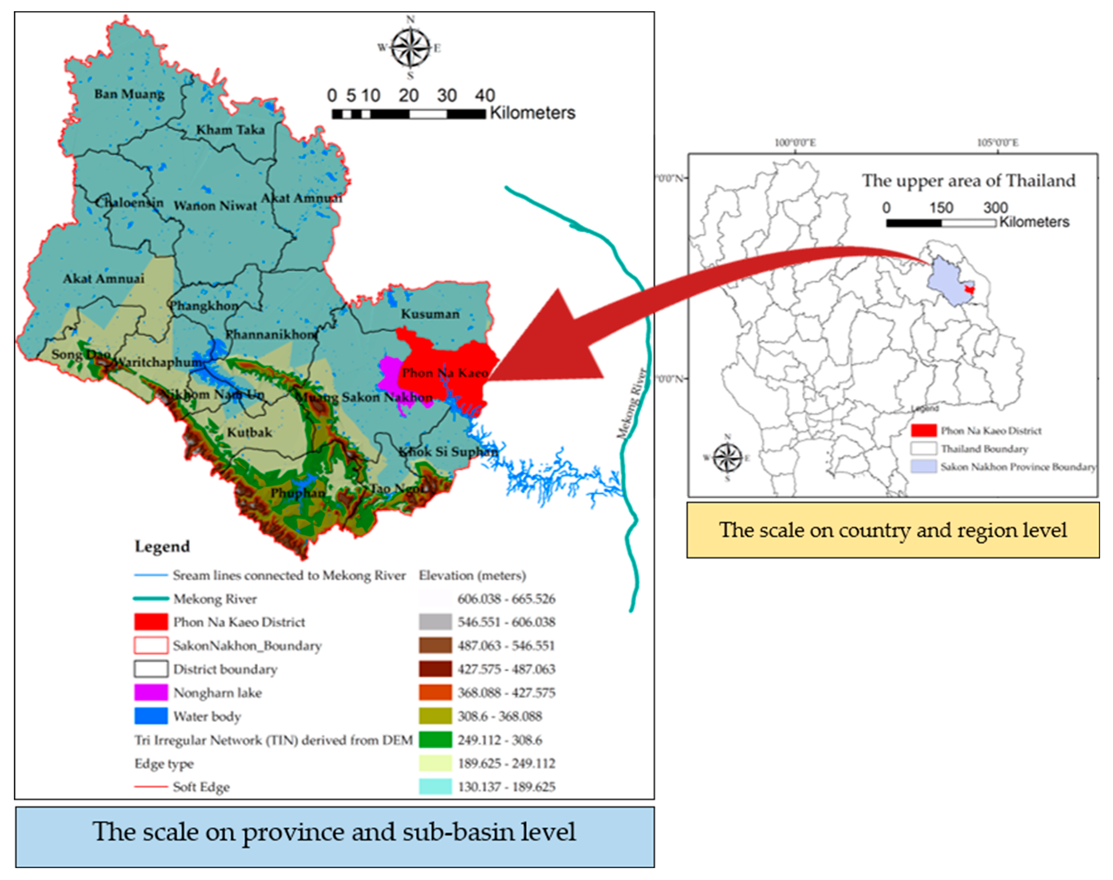
Figure 2. Percentage of people infected with liver fluke during 2019–2021 of the 8^th Regional Health Province (R8) near the Mekong River (adapted from R8, [75]).

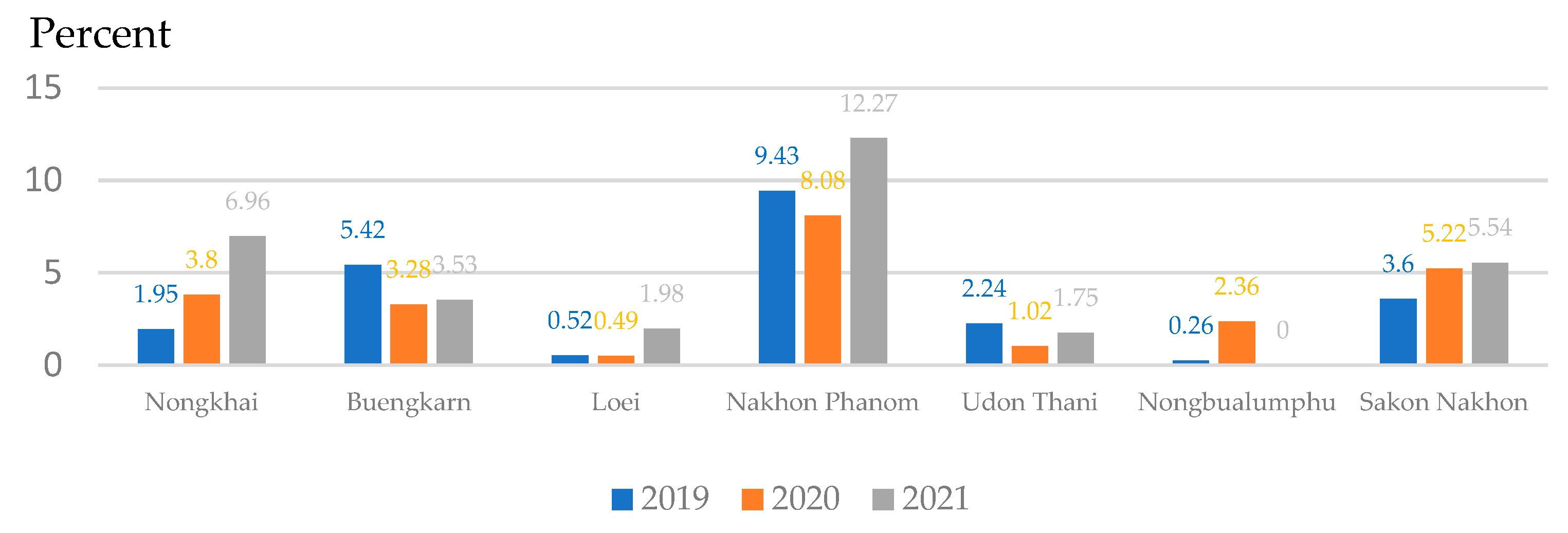
Figure 3. (a) A number of infected populations of each village with population density (persons/sq.km.). (b) Infected percentage of each village and percentage average of infectious in each sub-basin.

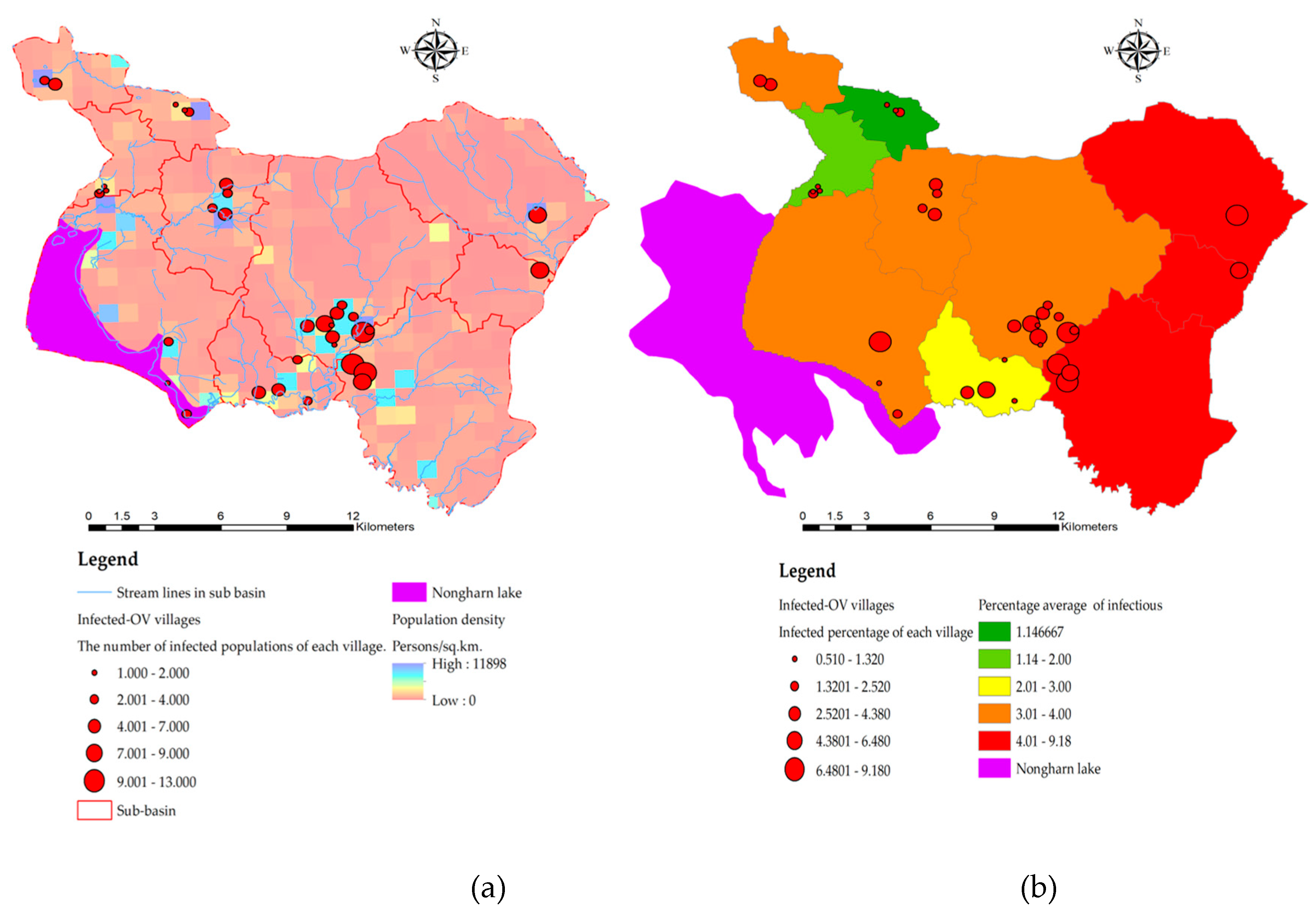
Figure 4. The framework of OLS modeling finds the relationship of liver fluke occurrence to spatial factors with the sub-basin level.

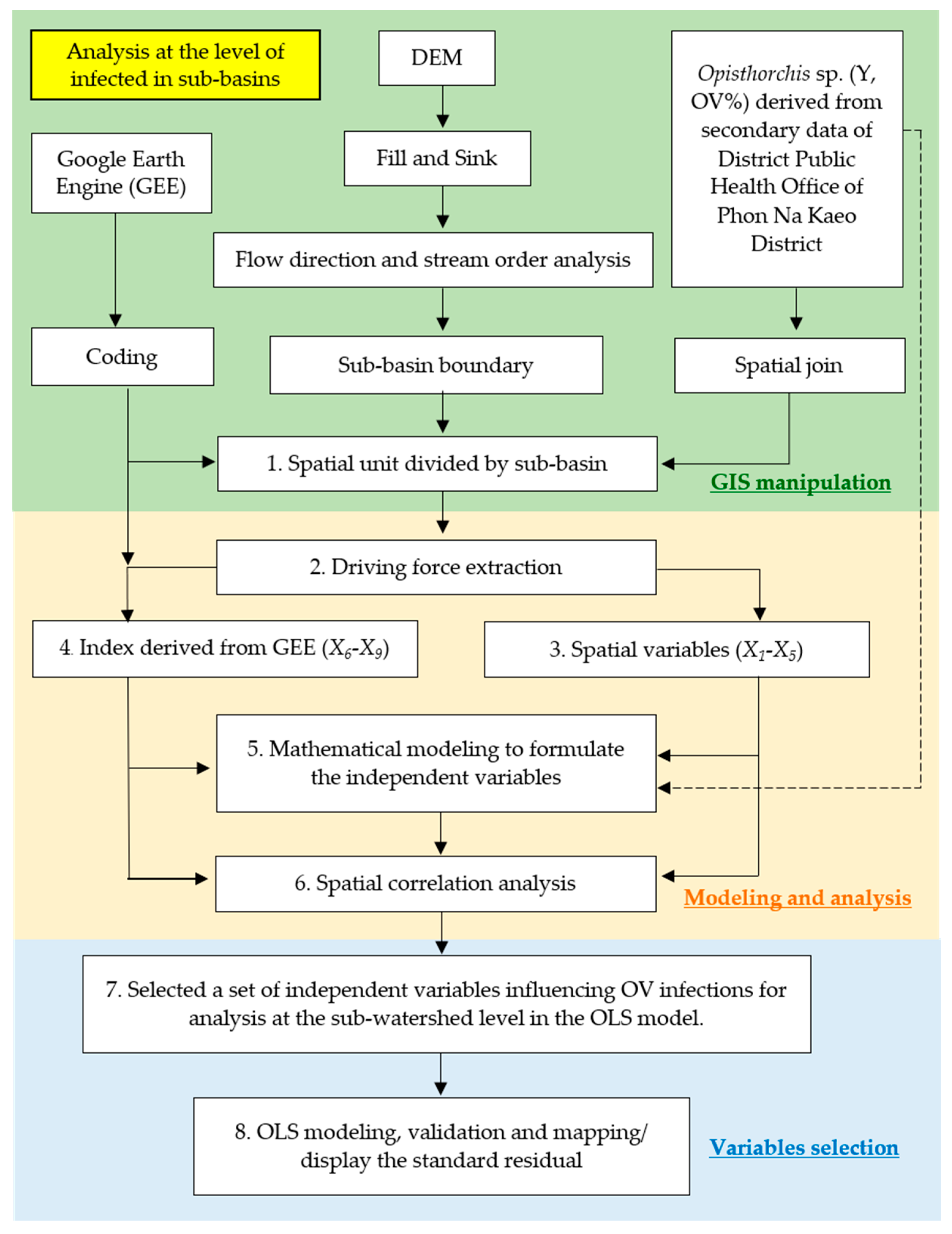
Figure 5. The forest-based classification and regression (FCR) for Liver Fluke (Opisthorchis viverrini) Infection prediction.

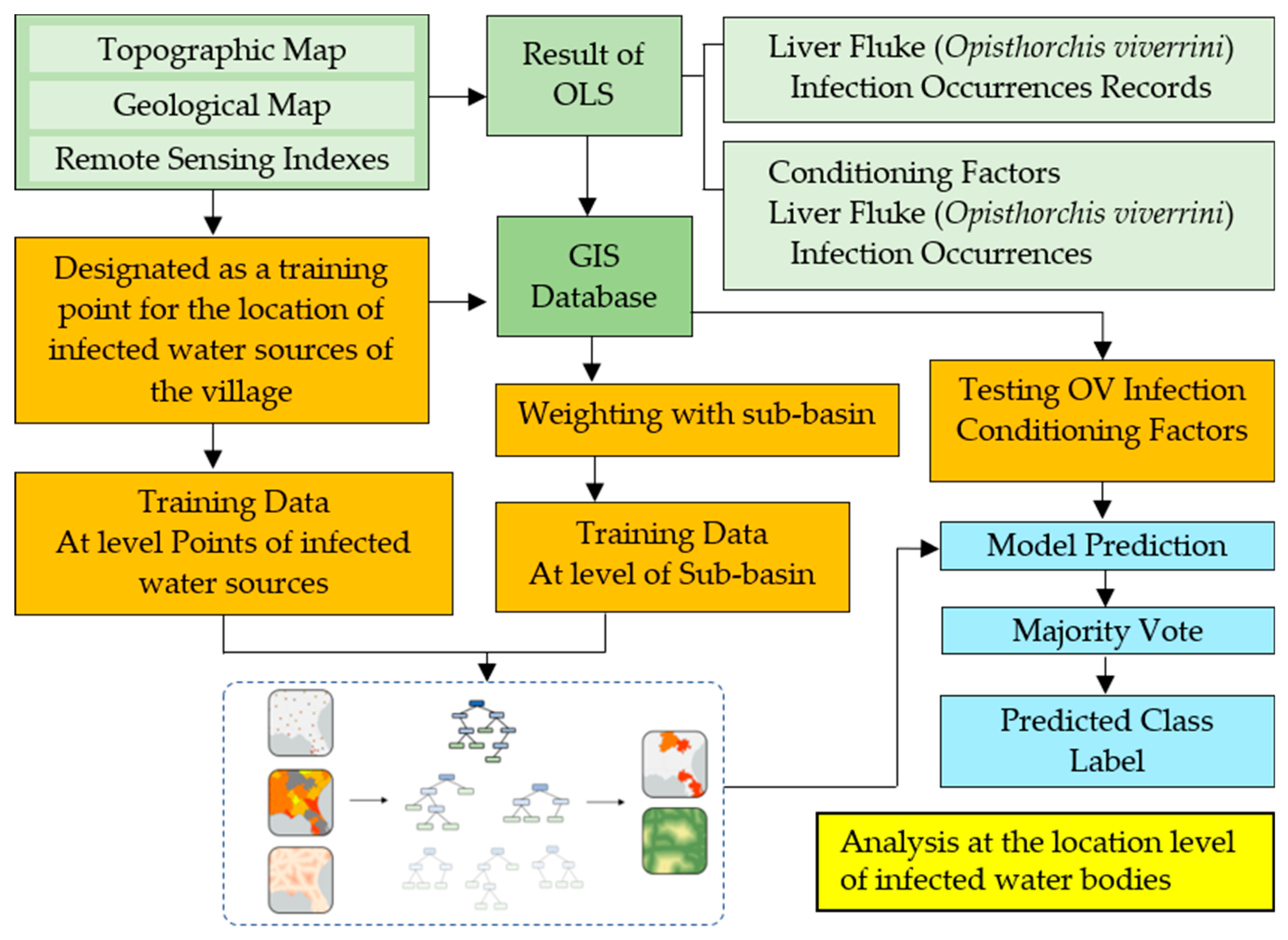
Figure 6. Sub-basin boundary map obtained from analysis of DEM data.

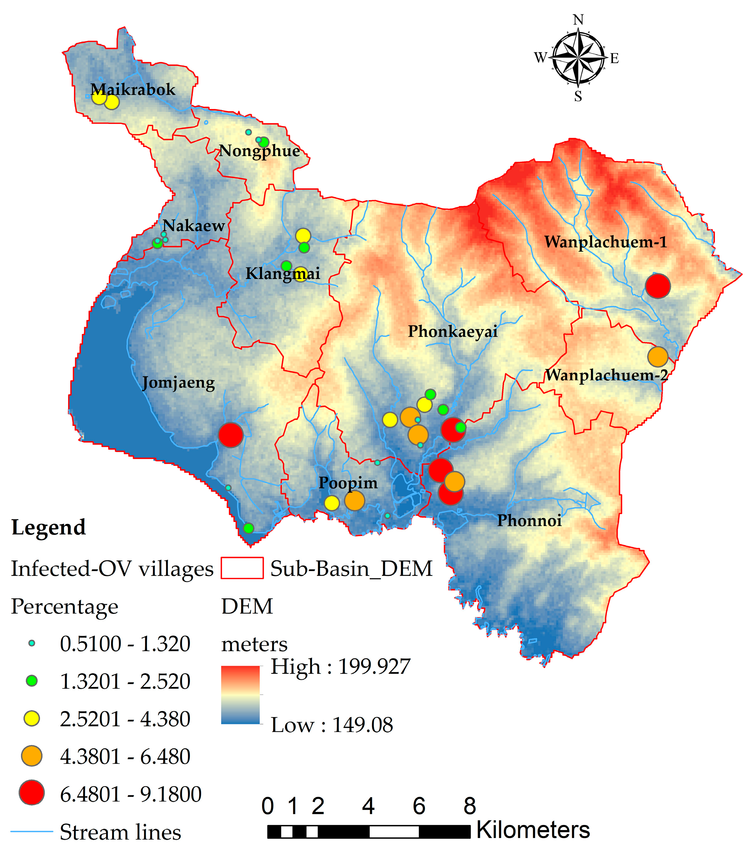
Figure 7. Raster mapping radius of OV-infected points using a heatmap: (a) radius 2 km, (b) radius 4 km.

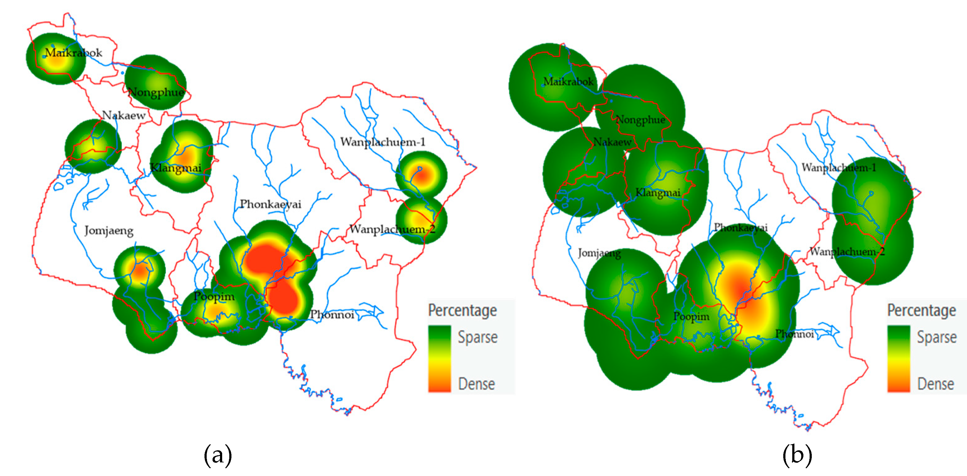
Figure 8. Map of independent variable indexes X₁ through X₉ generated using mathematical models, where (a) is X₁, (b) is X₂, (c) is X₃, (d) is X₄, (e) is X₅, (f) is X₆, (g) is X₇, (h) is X₈, and (i) is X₉.

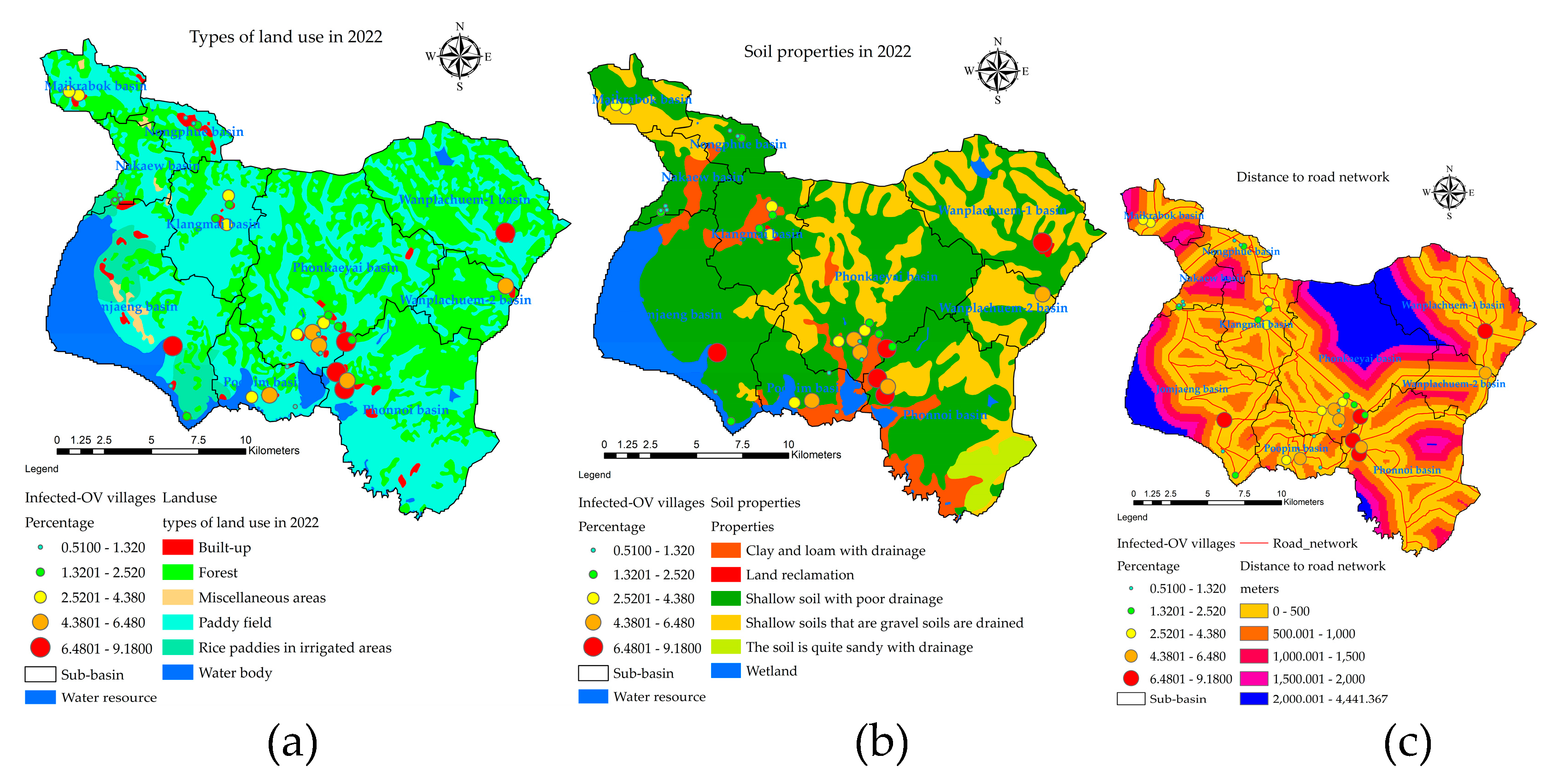
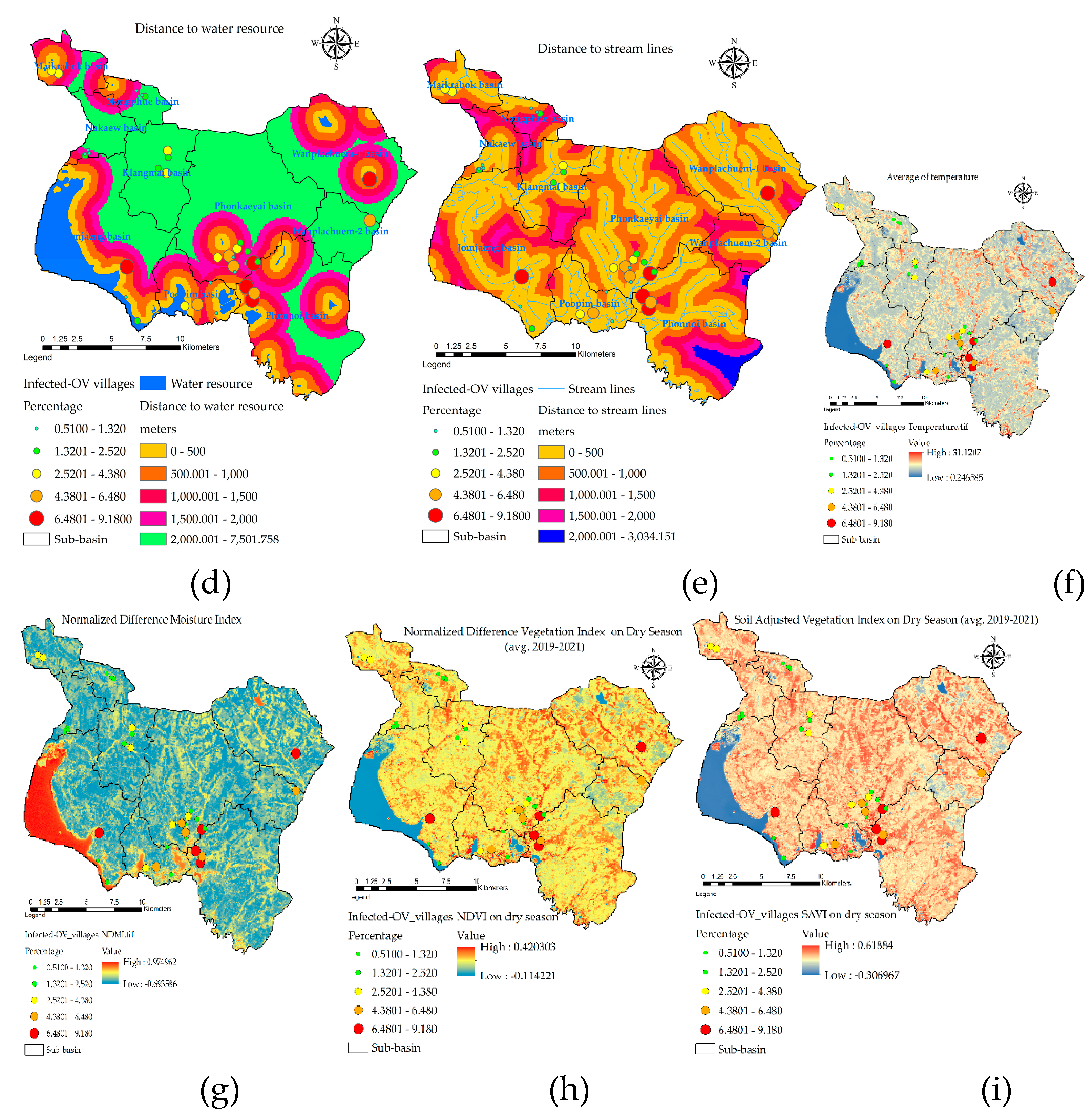
Figure 9. Pareto plots for screening sub-basin area units in determining the location of machine learning for importing Forest-based classification and regression models: (a) Y(% of OV), (b) X1 (Land use), (c) X2 (Soil), (d) X3 (Road), (e) X4 (Water), (f) X5 (Stream), (g) X6 (Surface Temperature), (h) X7 (NDMI), (i) X8 (NDVI), and (j) X9 (SAVI). .

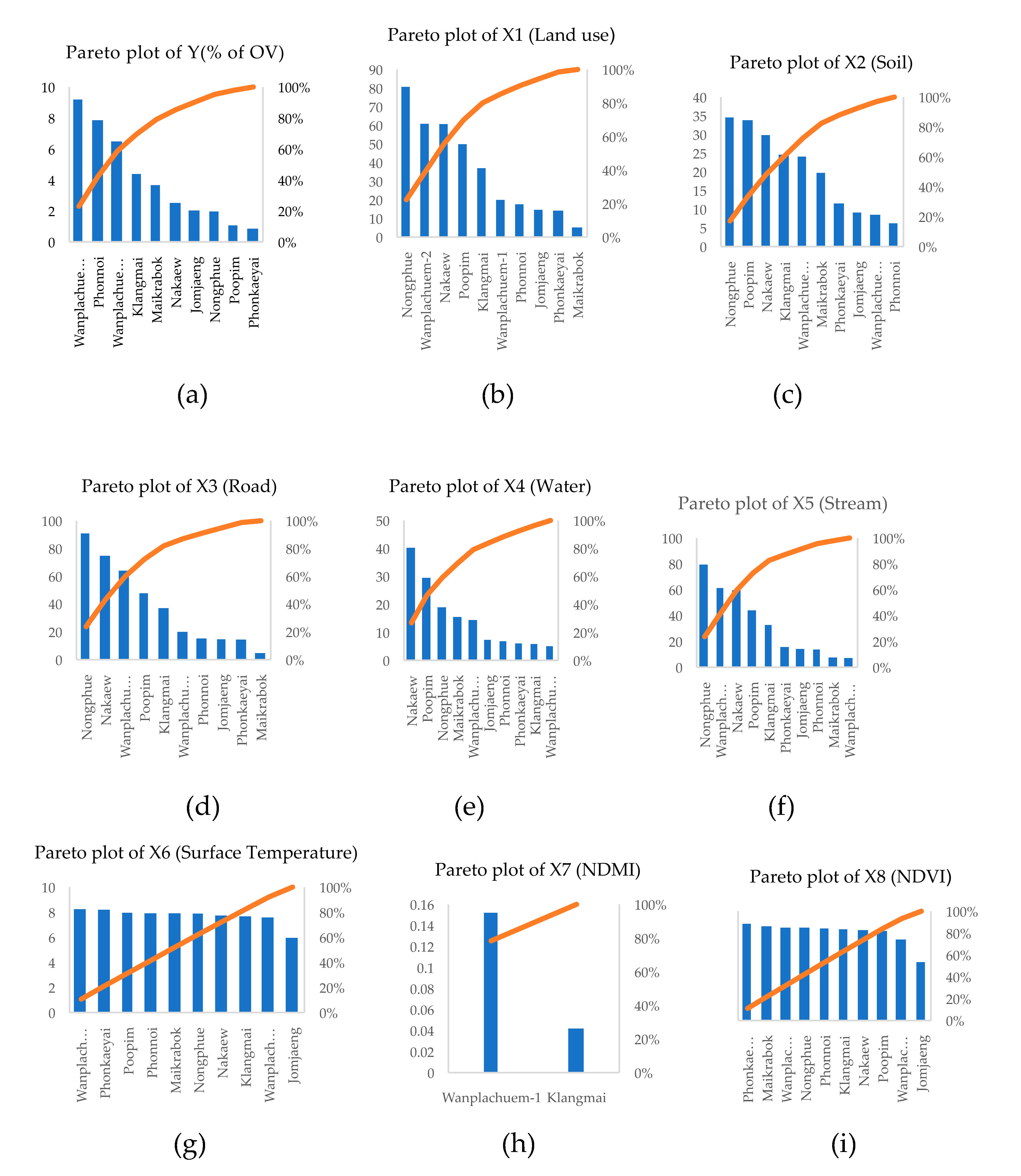
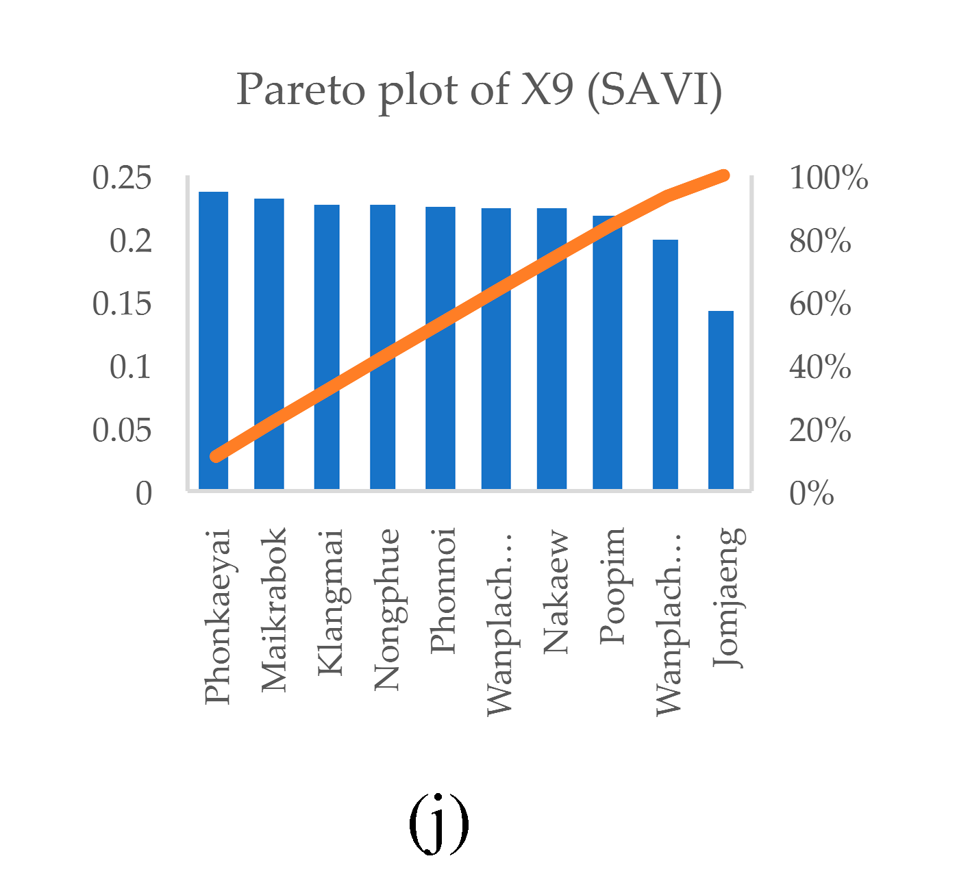
Figure 10. Residual plot and fit plot graphs of variable correlation X₅ (a1), (a2); X₆ (b1), (b2); X₇ (c1), (c2); X₈ (d1), (d2); and X₉ (e1), (e2) selected from correlation analysis.

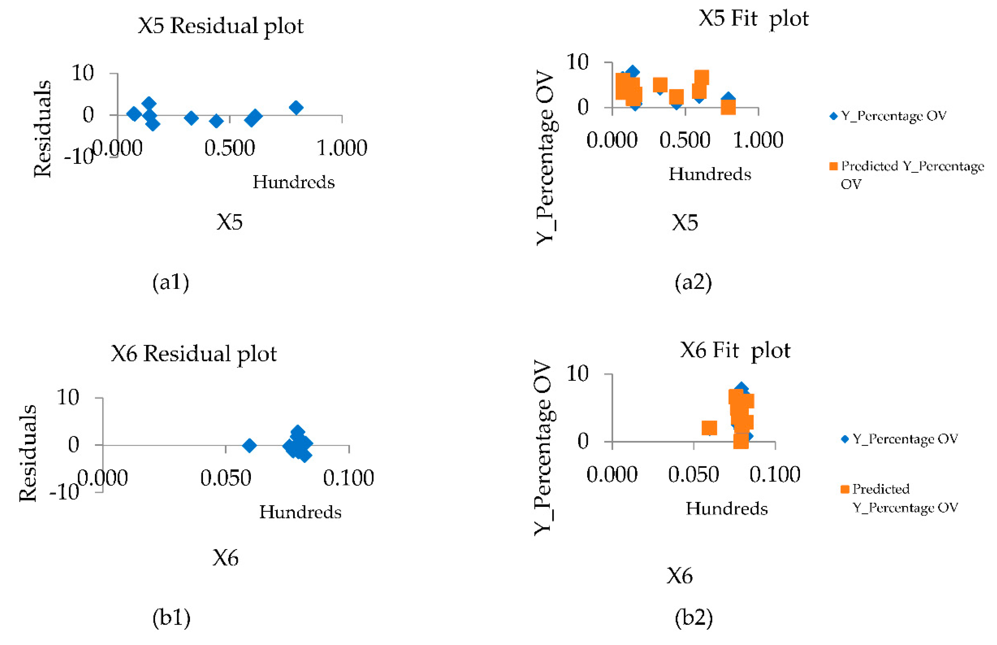
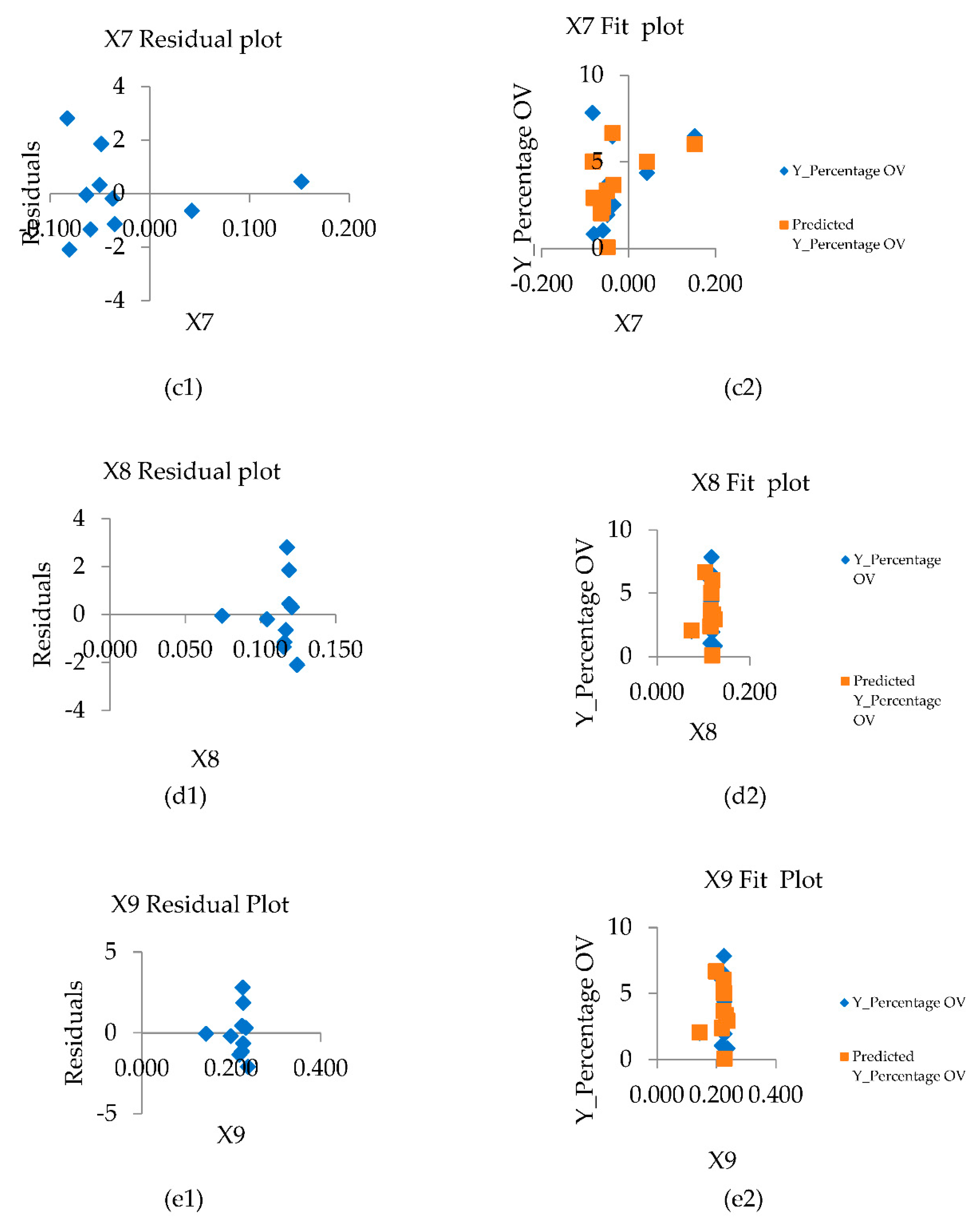
Figure 11. Comparison of standard residual of OLS alternative models: (a) OLS model 1, (b) OLS model 2, (c) OLS model 3, and (d) OLS model 4.

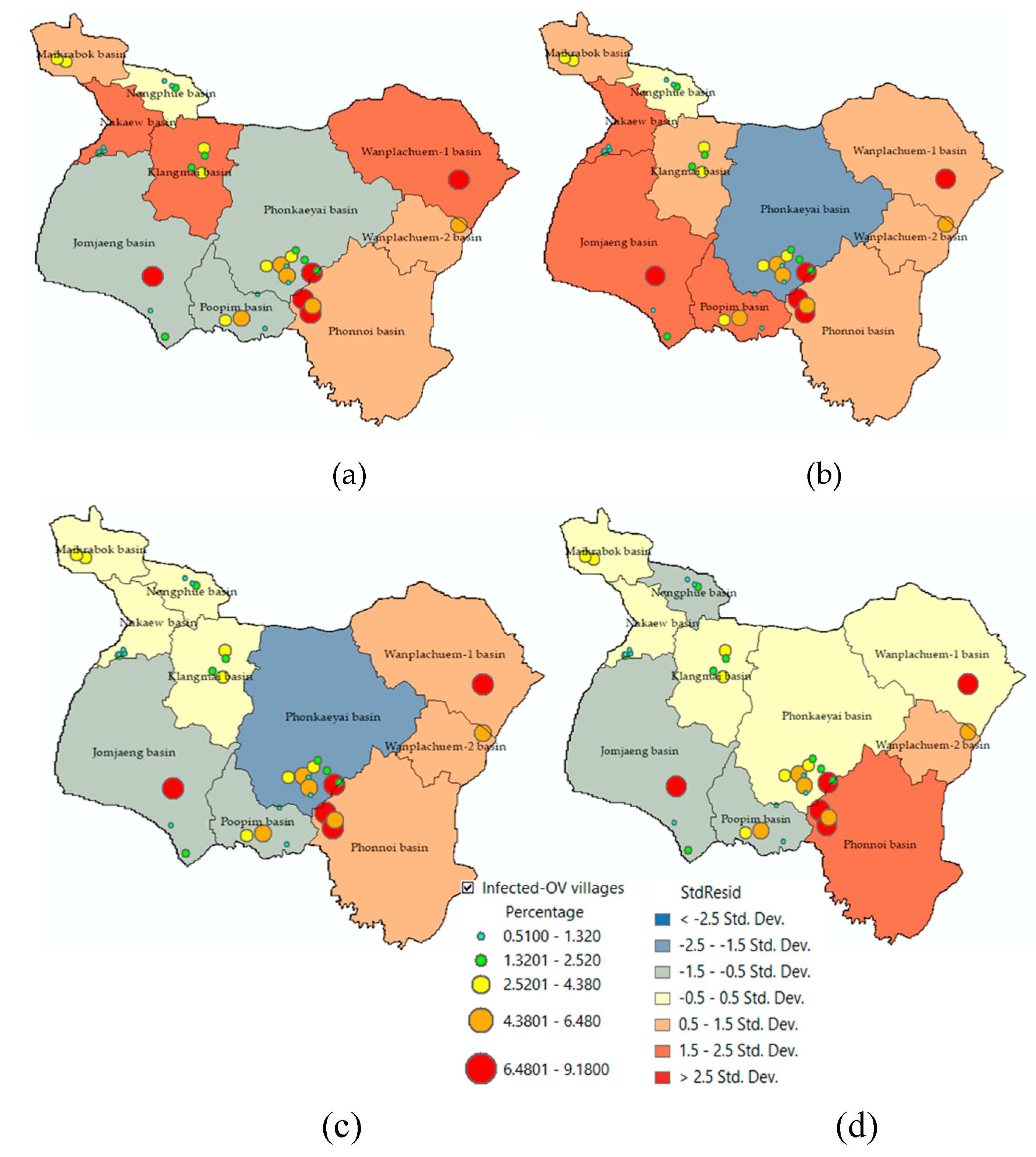
Figure 12. The whole dataset training, and testing.

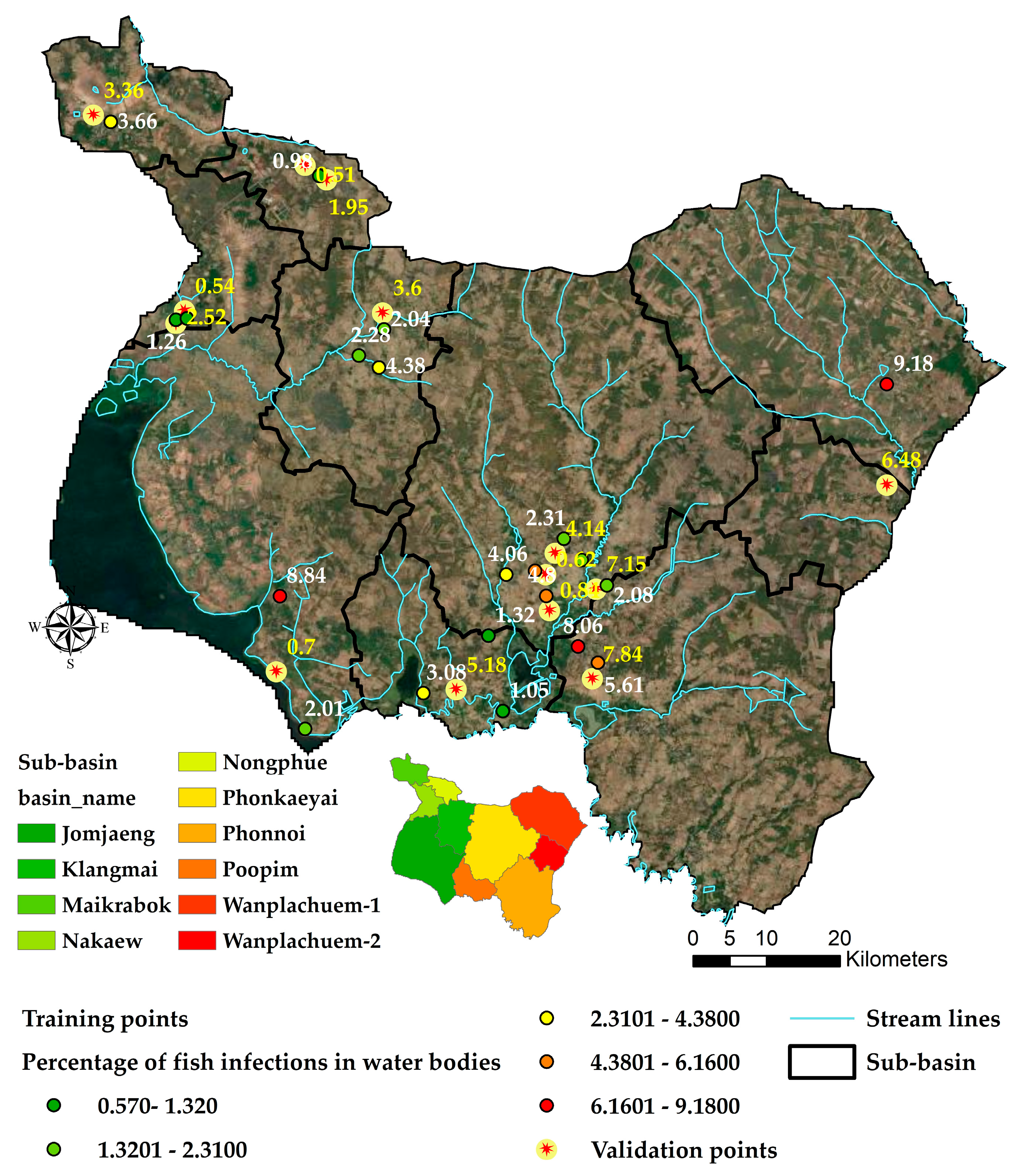
Figure 14. The results of prediction of FCR model 1 to model 4: (a) model-1, (b) model-2, (c) model-3, and (d) model-4.

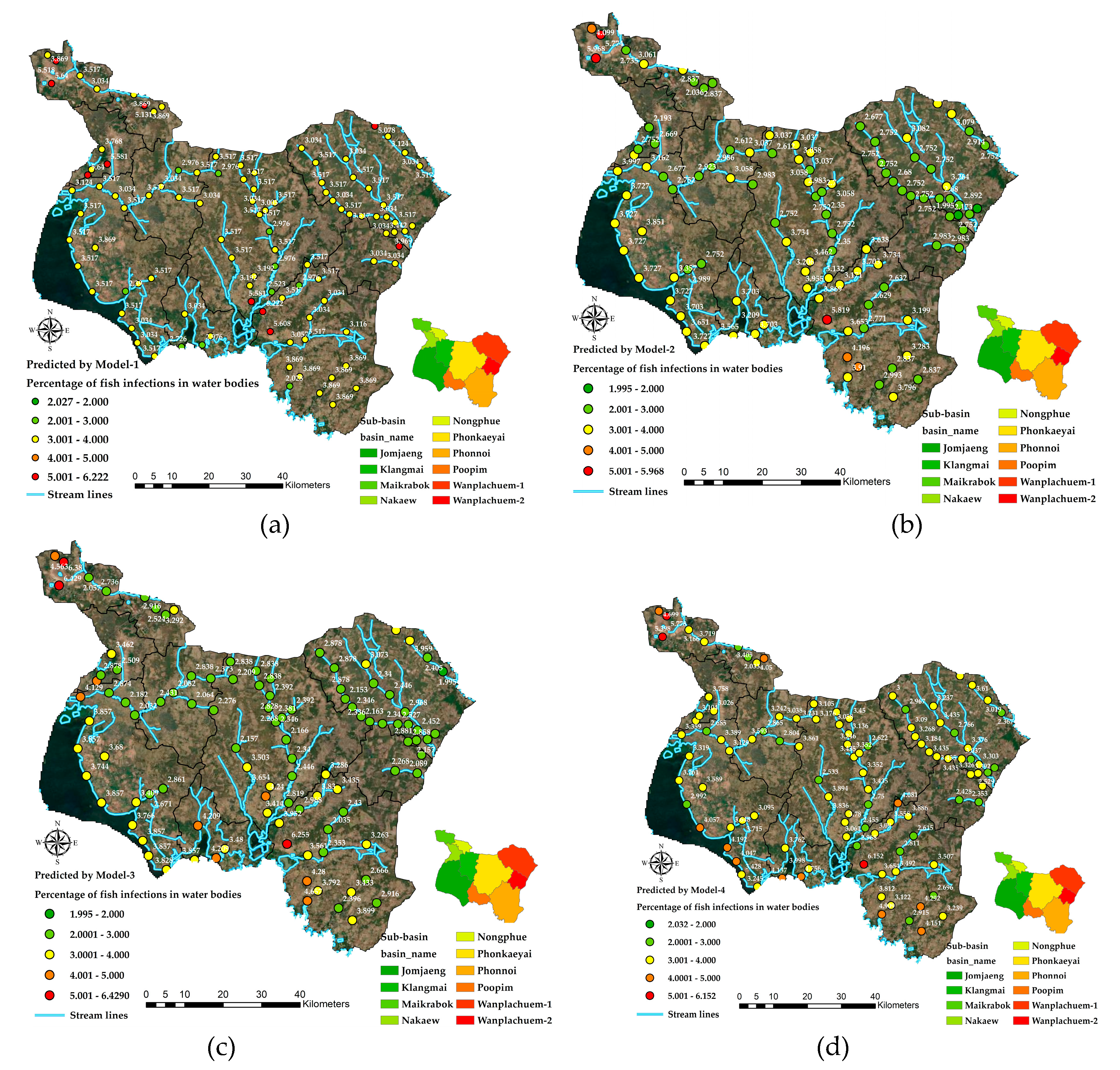
Table 1. Comparison of number of people with cholangiocarcinoma in 2019/2020. [72].

Provinces	Number of people with	Number of people with
	cholangiocarcinoma in 2019	cholangiocarcinoma in 2020
Nongkhai	22	37
Buengkarn	8	7
Loei	54	84
Nakhon Phanom	7	10
Udon Thani	50	88
Nongbualumphu	19	12
Sakon Nakhon	161	130

Table 2. The correlation between independent variables (X₁ to X₉) and dependent variables (OV-infection percentages) for analysis of OLS-modelled variable groups.

	Y(% of OV)	X₁(lu)	X₂(soil)	X₃(road)	X₄(water)	X₅(stream)	X₆(Temp)	X₇(ndmi)	X₈(ndvi)	X₉(savi)
Y(% of OV)	1.000	-	-	-	-	-	-	-	-	-
X₁	-0.167	1.000		-	-	-	-	-	-	-
X₂	-0.437	0.826	1.000	-	-	-	-	-	-	-
X₃	-0.189	0.992	0.813	1.000	-	-	-	-	-	-
X₄	-0.402	0.599	0.739	0.635	1.000	-	-	-	-	-
X₅	-0.226	0.985	0.838	0.984	0.612	1.000	-	-	-	-
X₆	0.173	0.116	0.184	0.106	0.109	0.067	1.000	-	-	-
X₇	0.395	0.060	-0.143	-0.061	-0.258	-0.193	0.243	1.000	-	-
X₈	0.082	0.092	0.227	0.095	0.134	0.062	0.969	0.171	1.000	-
X₉	0.079	0.097	0.242	0.103	0.144	0.074	0.950	0.150	0.997	1.000

Table 3. The OLS alternative modeling results.

Alternative OLS models for OV-predicted in watershed level	Independent variables	Coefficients	t-Stat		R²
Y(%OV1)	Intercept	0.465	4.373***	0.000***	0.524
	X₈(ndvi)	-1.534	-0.878 n/s	0.226 n/s
	X₉(savi)	-6.032	-2.212 n/s	0.125 n/s
Y(%OV2)	Intercept	4.528	1.975***	0.000***	0.672
	X₇(ndmi)	1.125	0.769 ***	0.044 ***
	X₈(ndvi)	-3.116	-0.890 ***	0.023 ***
	X₉(savi)	-9.852	-2.326 n/s	3.024 n/s
Y(%OV3)	Intercept	62.042	3.031***	0.000***	0.713
	X₅(stream)	-5.047	-2.068***	0.048***
	X₇(ndmi)	4.246	1.875 ***	0.034 ***
	X₈(ndvi)	-9.874	-2.661***	0.021***
Y(%OV4)	Intercept	57.410	0.979***	0.000***	0.681
	X₅(stream)	-0.0350	-3.462***	0.031***
	X₆(temp)	20.210	0.734 n/s	1.263 n/s
	X₇(ndmi)	7.220	0.540 ***	0.044 ***
	X₈(ndvi)	-1524.360	-0.548 ***	0.026 ***
	X₉(savi)	-2732.160	-2.356 n/s	0.895 n/s

*** = significant at 5% level. n/s = not significant.

Table 4. The model out of bag errors.

Model Out of Bag Errors	Model-1		Model-2		Model-3		Model-4
Number of Trees	50	100	50	100	50	100	50	100
MSE	10.203	8.98	7.298	7.074	9.075	8.93	10.203	8.98
% of variation explained	-46.689	-29.111	-5.511	-2.267	-33.117	-31.003	-46.689	-29.111

Table 5. The top variable importance.

Top Variable Importance	Model-1		Model-2		Model-3		Model-4
Variables	Importance	%	Importance	%	Importance	%	Importance	%
distance to stream lines	105.09	100	52.72	47	34.91	37	23.18	22
distance to water			58.75	53	32.32	34	39.7	37
ndmi					27.89	29	20.32	19
ndvi							22.79	22

Table 6. The explanatory variable range diagnostics.

Explanatory Variable Range Diagnostics	Training		Validation		Share
	Minimum	Maximum	Minimum	Maximum	Training^a	Validation^b
Model-1 distance to stream lines	0.48	1055.51	133.04	610.29	1	0.45*
Model-2 distance to stream lines	0.48	1055.51	594.64	610.29	1	0.01*
distance to water resource	108.65	6054.45	970.21	1604.04	1	0.11*
Model-3 distance to stream lines	0.48	1055.51	195.81	527.24	1	0.31*
distance to water resource	108.65	6054.45	1319.44	1756.75	1	0.07*
ndmi	-0.13	0.14	0.04	0.1	1	0.20*
Model-4 distance to stream lines	0.48	928.08	610.29	1055.51	0.88*	0.34*
distance to water resource	108.65	6054.45	1243.77	1604.04	1	0.06*
ndmi	-0.13	0.1	0.07	0.14	0.85*	0.10*
ndvi	0.05	0.16	0.17	0.18	0.82*	0.00*

(a) % of overlap between the ranges of the training data and the input explanatory variable. (b) % of overlap between the ranges of the validation data and the training data. * Data ranges do not coincide. Training or validation is occurring with incomplete data. + Ranges of the training data and prediction data do not coincide and the tool is attempting to extrapolate.

Disclaimer/Publisher’s Note: The statements, opinions and data contained in all publications are solely those of the individual author(s) and contributor(s) and not of MDPI and/or the editor(s). MDPI and/or the editor(s) disclaim responsibility for any injury to people or property resulting from any ideas, methods, instructions or products referred to in the content.

© 2023 by the authors. Licensee MDPI, Basel, Switzerland. This article is an open access article distributed under the terms and conditions of the Creative Commons Attribution (CC BY) license (http://creativecommons.org/licenses/by/4.0/).

Copyright: This open access article is published under a Creative Commons CC BY 4.0 license, which permit the free download, distribution, and reuse, provided that the author and preprint are cited in any reuse.

Downloads

146

Views

Comments

Subscription

Notify me about updates to this article or when a peer-reviewed version is published.

MDPI Initiatives

Important Links

Choose an area of interest and we will send you notifications of new preprints at your preferred frequency.

Disclaimer

Machine Learning-Based Forest Classification and Regression (FCR) for Spatial Prediction of Liver Fluke (Opisthorchis viverrini) Infection in Small Sub Watershed

Abstract

Keywords:

Subject:

1. Introduction

2. Materials and Methods

2.1. The Study Area

2.2. Datasets and Analyses

2.3. Independent variable modeling

2.4. Ordinary Least Square (OLS) approach for spatial modeling (analysis at the level of infected in sub-basins)

2.5. Forest-Based Classification and Regression (Analysis at the location level of infected water bodies)

3. Results

3.1. Mapping of The Spatial OV Infection (Y, Dependent Variable)

3.2. Mapping of The Independent Variables

3.3. Spatial Analysis of Factors Associated with Spatial Liver Fluke (Opisthorchis viverrini) Infection

3.4. Optimal OLS Model for Predicted with Liver Fluke (Opisthorchis viverrini) Infection (Watershed level)

3.5. Spatial prediction of OV-Infection using Forest-based Classification and Regression (FCR) (Location level)

3.6. Spatial Prediction of OV-infected

4. Discussion

4.1. Redundancy of Independent Variable Sets

4.2. Limitations of Spatial OLS Model

4.3. FCR Improvement Approach for Spatial Prediction

5. Conclusions

Author Contributions

Funding

Institutional Review Board Statement

Informed Consent Statement

Data Availability Statement

Acknowledgement

Conflicts of Interest

References

MDPI Initiatives

Important Links

Subscribe