
Submitted:
21 August 2023
Posted:
23 August 2023
You are already at the latest version
Abstract
This study aims to identify the model that best approximates the credit spread that should be fixed on debt instruments issued by both public and private companies, considering the particularities of the Mexican market. Five models were analyzed: Merton's [1], those proposed by Denzler et al., the one presented in this paper, which includes the conformable derivatives, taking as a reference the change of variable made by Morales-Bañuelos et al., and the Corporate Default Risk Model (DRSK) for Publics Firms of Bloomberg [4].
The required financial information was obtained from the Bloomberg platform, from which the probabilities of default, credit spreads, and credit ratings for each company in the sample under the model (DRSK) were extracted directly. Likewise, the program developed by Moody's K.M.V. was used to obtain the EDF (Expected Default Frequencies). It was concluded that the Modified Merton model approximates to a greater extent the credit spreads that fix on a prime rate on the loans granted to the Mexican non-financial companies.
Keywords:
Merton Model
; Brownian Model
; Power Law
; Brownian Motion Model
; Bloomberg Default Frequencies
; Expected Default Frequencies
; Conformable Derivates
; K.M.V. Moody’s
; Default Neutral Risk
MSC: 35R11; 91G29
1. Introduction
Analyzing a firm's financial performance requires a thorough evaluation of its financial health and knowing its strengths and weaknesses. This, in turn, leads to adequate decision-making and adaptability to the ever-changing business environment. See [5]. Firms must be willing to pay the market price of whatever goods and services they employ in their economic activities, irrespective of their field. All these expenses, in turn, must be financed balanced, allowing for present performance and future development. As is well known, there are three primary sources of financial resources: inner resources generated by the firm during its activities, cash inflows coming from stakeholders, and financial resources obtained using debt, be it short or long-term. As a rule, the debt ratios of a firm will depend not only on the goods and services it produces or distributes but also on the stage of the business development plan, the type of market within which it operates, and legal and fiscal restrictions, among others.
The interest rate governing such debts is often determined using credit scores from rating agencies such as Moody’s Investor Service (henceforth Moody’s). This score will often also define the yield a bond emitted by the company should offer. Put in other words, we could say that, in general lines, a firm's credit rating determines the opportunity cost of debt facing it. Nonetheless, credit ratings are often restricted to public companies with greater purchasing power, which leaves smaller firms with the complicated task of evaluating the real opportunity cost of debt. This is the case for many Mexican firms. The overall proportion of public firms in the Mexican market is relatively small. Further complicating this matter is a debt between peers, which can hardly be graded or rated, and a credit spread could be fixed outside the scope of the market value principle. Consequently, a new methodology called for the cost of debt to be directly proportional to the default risk.
Merton’s model in [1] can be used to directly estimate the risk-neutral default probabilities and the credit spreads to be added to the base interest rate. Also, the Brownian Motion Model (BM) and the Power Law Brownian Motion Model (PLBM) of [3] allow the estimation of the risk-neutral default probability and, thus, the credit spreads using the default frequencies. These models share features with both structural and reduced-form settings. In this work, we use these three models to estimate the cost of debt in different loans. Moreover, we propose a novel, modified Merton’s model to the same end and analyze and compare all four models. Our application focuses on Mexican firms. It is worth noting that there is no secondary corporate debt market in Mexico and no public data on loan recovery rates or credit ratings. To establish this comparison, we follow the definitions in [6] to estimate the rate of loan recovery where needed.
The modification we propose to Merton’s model consists of incorporating the conformable derivatives in the company's market value into the partial differential equation, effecting a change of variables, and then solving the equation to arrive at the traditional Black-Scholes and Merton solution.
The rest of the paper is organized as follows: Section 2 reviews the existing literature. Section 3 gives a theoretical presentation of all the models used in the analysis and introduces the modified Merton’s model. Section 4 presents the results of our empirical study of Mexican firms. Finally, in Section 5, we offer our conclusions.
2. Literature Review
According to [7], the development in advanced economies indicates business management's success in increasing firms’ performance. Also, following [8], corporate performance bears a causal link with the results of a firm, but an exact formula to compare the success of a corporate firm, be it with its past results or those of other firms, does not exist. For this reason, financial ratios, including debt indicators [10], are a primary tool for assessing a firm as they help assess financial health [9]. Debt ratios determine to what extent external and internal resources are financing a firm and help evaluate the risk of default.
The probability of default is itself determined by several factors, including the size of the firm, its industrial sector, whether it pays dividends, the fiscal policy in the country where it operates, the inflation rate, interest rates, exchange rates, and the overall economic outlook, among others. According to [11], models that employ data to predict the occurrence of a default event have evolved into three distinct types: structural, reduced form, and mixed. The first group, pioneered by Merton [1], based their calculations on the firm's market value. This model uses the Black-Scholes option pricing model to approximate the firm's market value. It then uses this information to model default and compare how likely a firm will incur it.
The reduced-form models do not explicitly include the default and firm characteristics relationships. Default is viewed as an accidental, unanticipated event that can result from diverse situations in the financial and economic markets. This way, an exogenous factor is included to help model default. This exogenous factor is often modeled as a jump process or is driven by some underlying stochastic process [11].
Research on the relation between the probability of default and the credit spread includes that of Eberhart [12]. The author studied the models by Merton [1], Leland [13], and Anderson et al. [14] and concluded that Merton’s model strongly and consistently underestimates the credit spread. In contrast, the other two models offer a better fit for accurate data on credit spreads. Also, Ericsson and Reneby [15] concluded that the risk of default and the liquidity premium are correlated with significant variations in credit spreads. The authors see this relation as causal. On the other hand, more minor variations in the credit spread do not seem to be highly correlated with the probability of default. They are mostly considered the effect of unknown and unmodelled factors: statistical noise. Another study by Teixeira [26] showed that Merton’s model overestimates bond prices by approximately 11% and underestimates credit spreads by 76%.
Finally, Eom et al. [16] tested and compared five models conventionally used to price bonds and corporate firms, namely, those by Merton [1], Geske [17], Longstaff and Schwartz [18], Leland and Toft [19], and Collin-Dufresne and Goldstein [20]. The authors show that using stochastic interest rates in the models does not significantly affect their valuations' accuracy. They also argue that all the proposed models are prone to substantial prediction errors, but the errors vary in magnitude and sign among the models. More specifically, when used on safer bonds (low leverage and volatility), all the models underestimate the credit spreads, and the opposite is true for riskier bonds. It is worth noting that Geske’s model outperforms Merton’s by including different kinds of debt. On the other hand, Leland and Toft’s model overestimates credit spreads, and this phenomenon does not seem solvable by parameter variation. Finally, it is seen that the assumptions on the recovery rates may strongly affect the prediction variance for the credit spreads.
Anderson and Sundaresan [14] studied reduced-form models, making some limitations evident. They argue that such models i) strongly depend on the functional form chosen and ii) do not consider other firms. Specifically, market risk and how it correlates to any given firm is separate from the model compared to the reduced form and structural models shown in [11]. The authors argue that by treating default as an accidental, unexpected event, reduced-form models lose focus on the firm’s structure, balance sheet, etc. Focused on computing the default and probability rates using observed market credit spreads, these models neither depend upon nor provide an economic or financial insight regarding default.
The PLBM was seen to better approximate the credit spread in an empirical study by Denzler et al. [2]. Model accuracy and quality were evaluated by comparing the results obtained using each model with the observed spread through a measure henceforth denoted by G.
The existing literature is consistent in its conclusions. However, it must be considered that these studies are primarily based on fully developed and stable economies and financial markets. The problem of evaluating these models in emerging economies is still open. This paper addresses this problem and includes a novel model based on Merton’s model of [1] and conformable calculus.
3. Materials and Methods
This section describes the theoretical models that estimate credit spreads using default probabilities as input. We describe the following models: Merton’s and Vasicek-Kealhofer's (VK), Brownian Motion (BM), Power Law Brownian Motion (PLBM), Corporate Default Risk Model for Public Firms, and Modified Merton’s. Following the financial theory, the cost of debt should be directly related, among other factors, to the financial situation of the entity issuing it, the economic landscape of the country in which it operates, and the features of the industry sector it belongs. All these factors should, therefore, be reflected by the interest rate at which the debt is bought.
Following Crosbie and Bohn [27], the risk of default is defined as the uncertainty that a firm may not have the means to pay its debt. However, before the facts, there is no exact way to determine if a given firm will or will not default in each period. Estimating default probabilities becomes an important endeavor. It is well known that due to this uncertainty, firms are compelled to offer a risk premium, i.e., an excess return when compared to the risk-free interest rate, and that this risk premium is, broadly speaking, directly proportional to the probability of default.
From an accounting point of view, the risk of default increases as the value of the assets approaches the book value of the debt since a firm default when the value of its assets is less than the total debt. Nonetheless, as was found by Crosbie and Bohn [27], the actual moment of default strongly depends on the ratio of short-term debt to long-term debt. According to the authors, the probability of default would be an increasing function of this ratio. To state this differently, remember that the relevant net value of a firm (Net Market Value) is obtained by subtracting the point of default from the total market value of its assets. Then, a firm is in default when its Net Market Value is equal to zero. A measure of the risk involved is, thus, the volatility of its assets or, more precisely, of the percentual change in its market price.
The former concepts can be combined into a single idea known as distance to default (DD) that compares the Net Market Value of a firm to its volatility using the formula:
The distance to default combines vital elements to estimate the risk of default: the market value of the firm’s assets and their volatility, and indirectly industry and firm risks, geographical risks, company size, and other factors that can be correlated to the market value of the assets. Using this measure, the probability of default can be estimated. Such estimation depends upon the probability distribution of the price of the firm’s assets but may also be derived from known empirical relations between default and DD.
3.1. Merton’s Model, Vasicek, and Kealhofer
We now briefly explain the model by Vasicek and Kealhofer in [5], henceforth abbreviated VK, which will serve as a preamble better to understand Merton’s model in [1]. The authors of [5] extended the option valuation model initially developed in [1] to compute default probabilities. Just as in Merton’s model, the firm's equity is considered a perpetual option in the VK model. The point of default acts as a barrier to the firm’s value; if the value of equity attains this value, the firm will no longer be able to pay its debts. Under this model, debt and equity are considered derivatives, with the firm’s value as the underlying asset.
According to [5], the default probability depends on six variables, namely, the current value of the firm’s assets, the probability distribution of said assets at time t, the volatility of the value of the assets, estimated using the VK model at time t, the point of default, the book value of the debt, the expected growth rate for the asset’s worth, and the time horizon. Also, according to [5], the default probability represents the possibility that the value of the assets is below the point of default, also known as Expected Default Frequency and abbreviated.
The users from Moody’s system can get the EDF. The platform predicts the yearly probability of default for the year to come. In Moody’s approach, the best grade for a firm or instrument is Aaa, meaning an almost certain payment or a practically null probability of default. Next are grade Aa, then A, Baa, Ba, B, and Caa, each representing a greater risk than its predecessor. To facilitate a finer analysis, each category has been segmented. We, thus, have Aa1, Aa2, Aa2, A1, A2, A3, and so on until reaching the riskiest Caa.
Having determined the EDF, the next step is mutating this probability into the credit spread to be added to the risk-free rate, considering the risk particular to the firm. More specifically, diverse methods exist to compute the credit spread, such as the Brownian Motion Model, the Power Law Brownian Motion Model, the Modified Merton model (proposed in this paper), and Merton’s Model.
According to Merton [1], the valuation of financial options can be applied to corporate instruments, such as actions and debt. In this scenario, the underlying asset corresponds to the value of the firm’s help, and the diffusion process to be used will be the Geometric Brownian Motion
Where μ represents the expected return on the firm’s investment, q is the rate of dividends, coupons, and interests paid by the firm to stakeholders, is the standard deviation on the value of the assets, and dZ represents integration concerning a traditional Wiener process.
Merton affirms, in [1], that a shareholder has a residual right on the economic flows generated by the firm. If the debt is due on t = 0, they will receive the difference between the free cash flow and the total amount of repayable debt. If a firm with assets for a value of V and nominal debt of B satisfies V > B, the shareholders will obtain a total of E = V – B. On the contrary, if B > V, the shareholder will not receive any cash flow since all V will be allocated to pay the debt. Finally, the shareholder gets nothing again if V = B, E = 0. As can be inferred, the value of a firm at time T equals the sum of its debt B and its equity capital E. Furthermore, equity can be compared to a call option on the value of the firm’s assets VT with an exercise price equal to B, since
It uses the Black and Scholes formula of [25] for the valuation of European options and taking as the volatility of the underlying , the variance of a company's returns and the market value of the company must be cleared by forming a system of equation.
Where V0 is the total market value of the firm’s assets at time t0, and VT represents the same value at time T. E is the market value of the dictionary capital at the initial time, B is the value of the interests and money to be paid at time T, r is the risk-free interest rate, represents the volatility of the firm’s assets (which are assumed homoscedastic). Furthermore, is the volatility of the shareholders’ equity, (*) is the standard normal cumulative distribution function, and T is the debt’s due date.
According to this model, the current value of the debt equals the difference between V0 and E0, and the risk-neutral default probability can be computed as (-d2). Knowing the market value of all the company assets and their volatility is necessary to add this probability. Unfortunately, these values are not directly observable or present in a firm's financial reports. However, if the firm is public, the market value can be computed by multiplying the number of shares times the market value per share, and its volatility can also be calculated.
This paper estimated the volatility using the GJR-GARCH model of [31], extending the traditional GARCH process by including asymmetries in the volatility. We obtain the following equations with these variables and follow Itô’s Lemma.
We get a complete system to obtain the unknowns uing these equations. The credit spread can be computed with these values, following the procedure in [27].
3.2. Brownian Motion Model (BM) and Power Law Brownian Motion Model
3.2.1. Introduction
Before explaining the BM and PLBM models, it is essential to detail the calculation of parameters used by both models, such as, among others, the annualized default risk-neutral probability, the recovery rate, and the credit spread.
Under an argument similar to that used in the valuation of financial options, Denzler et al. [2]] calculated the risk-neutral probability of default assuming that one has invested in two zero-coupon bonds, one risk-free and the other risk both with maturity date in. In the case of the risk-free bond, the flow to maturity is equal to the expected value of the flows of the risky bond multiplied by the risk-neutral probability of default and the recovery rate as shown below:
Where: E[F] is the expected value of F, a riskless bond at maturity, is the risk-neutral probability of default at time ti with maturity at Tj, and R is the recovery rate.
As expressed by Denzler et al. [2], the essence of pricing under risk neutrality is that both investments offer the same return, such that the expected value under the risk-neutral probability of default of a risky zero-coupon bond with maturity at Tj discounted at a market rate free of credit risk () is equal to the value of a risky bond discounted at a rate that includes default risk () equation (11). Substituting equation (10) into (11) and doing some algebra, we arrive at expressions (12) and (13).
It should be noted that represents the risk-neutral probability of default during the remaining term to maturity of the debt instrument, which in some cases can be greater or less than one year. Therefore, to perform some analysis, in [2], they suggest annualizing this probability as shown in equation (14), the credit spread can be obtained with the neutral probability of default as shown in (15).
Finale represents the base credit spread plus the credit risk-free rate. Where represents the base credit spread plus the credit risk-free rate.
The actual risk-neutral probability of default can be derived if the recovery rate (R) is known. Hull [6] defines a bond's recovery rate as the bond's market value immediately after default as a percentage of face value. In general terms, a generic value of 40% is assumed for all instruments based on empirical studies by Frye [21], Altman and Kishore [22], Acharya [23], and Hamilton [24]. Despite this, imposing a fixed recovery rate is different from reality since there is evidence that this recovery rate has significant variations concerning the average loan rate [24].
Hull [6], for his part, states that recovery rates are negatively correlated with default rates. In fact, in [24], they performed an analysis with data on U.S. bonds for the period from 1983 to 2004, arriving at the following linear relationship:
Average recovery rate= 0.52-6.9 x Average default rate.
The most appropriate way to calculate the credit spread would be to obtain the real recovery rate for Mexican entities according to the type of loan (senior or junior) or the credit rating; however, since this information was not available, the recovery rate was calculated using the conditional default probabilities.
According to Hull [6], conditional default probabilities represent the probability that an entity defaults between time t and t+∆t, given that it paid previously. This probability is called the default intensity at time t where represents the average default intensity between 0 and t. If we denoted the default probability at time t as Q(t), we obtained the default intensity with the equation (17).
If we denote the EDF as P(t) and assume that P(t)=Q(t), then we can define as shown in equation (18). On the other hand, Hull [6] proposes another way to calculate the neutral probability of conditional default per year, given that the entity did not default previously. This approach starts from the premise that the only reason why a corporate bond can be sold at a lower price than a risk-free bond with the same characteristics is because of the possibility of default in the payment of the former. Therefore, this probability of default would be calculated as shown in equation (19).
Where s is the corporate bond yield spread over the risk-free instrument, and R is the expected recovery rate. Now, if we consider the one-year EDF, as well as the definitions of given by equations (18) and (19), we can arrive at the following approximation of R (20).
The probability of default and the consequent credit spread cannot be readily determined for companies not listed on stock exchanges. Hence, Denzler et al. [2] suggest two models for calculating them: the Brownian Motion (BM) and the Power Law Brownian Motion (PLBM), which will be briefly explained below. These models, as mentioned by these authors, incorporate characteristics of the structural and reduced-form models.
3.2.2. Brownian Motion Model (BM)
The BM takes as its basis the valuation of debt instruments with the theory of financial options proposed by Black-Scholes [25] and Merton [1], as well as the migration models of credit ratings and credit transition probabilities (Markov chains). Denzler et al. [2] modeled the credit rating, as well as the distance to default () as a general Brownian motion, with an initial level equal to , such that , i.e.
Where: is the volatility of the process and is a Wiener process.
In [2], they also assume a minimum barrier corresponding to the default level d; once the company reaches this level, it cannot recover. To facilitate the calculation, this level is defined as zero and consequently, the initial level of is transferred. They also believe that the processtouches the level d during the entire instrument life. According to the formal development made by Karatzas and Shreve [27], The following proposition is established:
Proposition 1
. The probability of touching the default barrier during the interval [0,T] starting at
is as follows:
Inverting the above equation, the initial value of the processwould be equal to:
Where:is the maturity date of the debt instrument,is the probability or frequency of default (EDF) at maturity T,is the cumulative standard normal distribution andis the inverse cumulative standard normal distribution.
Proposition 2
. The actual probability of default at
is equal to:
Where:, is the expected default frequency (EDF) with maturity in one year and, is the expected default frequency (EDF) with maturity in.
In [2], they assume that the actual probbility eals the neutral probability default , since their objective is to derive the neutral default frequency, they obtain that this probability can be calculated as follows.
Where: corresponds to the expected annual default frequncy ( EDF) and is the neutral probability of default until maturity of the instrument at . This probability can be annualized by applying the equation (14).
According to the empirical analysis performed by Denzler et al. [2], it turned out that this model needs to describe sudden changes in credit rating adequately. Additionally, this model assumes that as the instrument approaches maturity, it loses rating, which is only sometimes valid in all cases.
Considering these deficiencies, in [2], they develop another model that considers the possibility of sudden changes in credit quality through a Gaussian diffusion model called the Power Law Brownian Motion Model (PLBM), which will be explained in the following section.
3.2.3. Power Law Brownian Motion Model (PLBM)
This model considers the possibility of sudden instrument degradation and credit rating asymmetry. The PLBM includes additional parameters to the previous equation arriving at (23).
Where: and are to be estimated at each point in time describes the empirical behavior of firms in the market. It captures mainly all movements (including explosive scaling law movements) of neutral probabilities wconcernnge due date aa describes the total expected level of default probabilities for the whole market; it can be interpreted as the market premium for credit risk.
In [2] they estimated both parameters at each point in time by running the following linear regression, considering all maturities of the instruments. Such that, is used as the independent variable and as dependent variable.
Where: is an independent random variable with y .
It is important to note that this formula directly calculates the risk-neutral probability of annual default, whereby the credit spread would be obtained by substituting the value of this probability in the equation presented above .
3.3. The Bloomberg Corporate Default Risk Model (DRSK) for Public Firms
The DRSK is a hybrid model combining a statistical approach with structural models. Bondolini et al. [4] use logistic regression to estimate the probability of default events based on factors that best capture credit risk. These factors are relevant accountings ratios- one of the critical factors is the distance to default (DD) (1).
As mentioned in the previous paragraph, the DRSK estimates real-world default probabilities (DP) using a logistic regression of historically realized defaults against the structural model DD and additional risk factors such as profitability and insolvency. Specifically, the real-world default probabilities for a firm at tenor modeled as
Where .
The model is calibrated by logistic regression of the model’s factors against the default indicator operation set. Using marginal DPs from the logistic regression, one can obtain cumulative DPs for each tenor in the years as follows in [4]. In the same way, annualized DPs can be obtained as follows in the equations (27) and (28).
The cumulative and annualized DPs are used by [4] to evaluate a firm's default probability per different horizons. They help compare and validate stylized facts between simples within different grades of credit quality.
The DRSK is calibrated to historical financials over 20 years period containing records for over 65,000 firms. The models achieve high-performance levels in adjusted pseudo-R squared (e.g., between 34% and 47%) [4]. The model DP is predictive of credit events up to a horizon of five years and tracks the realized default rates closely over time. According to Bondoli et al. [4], the model is responsive to market conditions; default probabilities drop during economic expansions and rise during economic contractions.
3.4. Modified Merton Model
3.4.1. Fractional and Conformable Derivatives
Fractional derivatives arise from the concern to generalize the n else a real or complex function.
Khalil, Al Horani, Yousef and Sababheh present a new definition of the fractional derivative whose objective is to facilitate the calculations, additionally they state that the fractional derivatives for 0<α<1, are local by nature. They also state that given a function and the conformable fractional derivative of f of order α is defined for all of order "n" from an integer to a non-integer, "n" can be a fraction, an irrational or a complex.
Khalil et al [30] present a new definition of the fractional derivative whose goal is to facilitate the calculations, additionally they state that the fractional derivatives for 0<α<1, are local by nature. They also state that given a function and the conformable fractional derivative of order is found to be defined as for all and . If f is α-differentiable in some , , and the there exist, it is defined . Similarly, Anderson, Camrud and Ulness [33], mention that if the conformable fractional derivative, denoted as or , exists, it is said to be α-differentiable, derived from which they present the following theorem.
Theorem 1
If a function f is α-differentiable in, then f is (29) at, consequently
To analyze the equivalence between conformable and fractional derivatives, Anderson et al. [32] and Morales-Bañuelos, Muriel, and Fernández-Anaya [3] apply only a change of variable, such that reaching the same result as Khalil et al. [30], as presented in equations (32) and (33).
In [32] have the following properties. This definition yields the following results (from Theorem 2,3 of Katugampola [33].
- , linearity
- =, product rule.
- , chain rule.
According to [32] to see the equivalence of the conformable derivate and the change de variable consider direct substitution and chain rule in
The steps followed by Morales-Bañuelos et al. [3] and Anderson et al. [33] to transform a traditional second-order linear differential equation, known by its acronym SOLDE (Second order linear differential equation) into a conformable one, by changing the variable are the following. Equation (30) in [3] and [33] obtain the expression shown in (34), and finally, they state the second order linear conformable differential equation as follows.
Now let
Therefore Eq. (34) becomes
3.4.2. Proposed Model
As mentioned above, the objective of this work is to solve the Black, Scholes, 3433444and Merton (BSM) partial differential equation [25] and [1] taking as a reference the change of variable proposed by Morales-Bañuelos et al. [3], to obtain an equation with which to calculate the credit spread, incorporating the conformable derivative in the firm value parameter.
Solving the Black, Scholes, and Merton Equation by conformable derivatives
Following the proposal of Morales-Bañuelos et al. [3], for the purpose of solving the traditional BSM partial differential equation [25] and [1], we are going to perform the change of variable in the signature value parameter, such and , such that 0<α≤1, and first derivative of the function of with respect to is equal equation (355)
Subsequently, the second derivative of the function of u, concerning u, was calculated, again incorporating the change of variabe , we arrive at equation (36). If these derivatives are substituted into the original equation developed by Black, Scholes, and Merton [25] and [1], the partial differential equation would be represented as shown in (37) and (38). According to [1] equation (36) is a parabolic partial ddifferentttrialeequationfforor, which must be satisfied by any security whose value can be written as a function of the value of the firm and time, like in this case.
Similarly, we examined the simple case of corporate debt pricing: a) a single class of debt and residual claim equity. We suppose in the same way as [1] that the indenture of the bond issue contains the following provisions and restrictions: 1) the firm promises to pay a total of F (Face Value antes previously denoted as B) to the bondholders on specific calendar date T; 2) in the event this payment is not met, the bondholders immediately take over the company (and the shareholders receive nothing); 3) the firm can not issue any new senior (or of equivalent rank) claims on the firm nor can it pay cash dividends or do share repurchase before the maturity of the debt. By definite harmful, we have the constraint presented in equation (39).
Clearly at time T, the firm will pay the bondholders if and the equity value will be the difference, otherwise, the shareholders receive nothing. So the final condition is , As mentioned by [1] this isomorphic price relasionship between levered equity of the firm an call option we can solve the equation as Black and Scholes [25] did, but including the parameter and variable changes: , the solution to the modified differential equation is shown in equations (40)
3.4.3. Test Parameter
In order to evaluate the fit of these models and to be able to subsequently perform inference, with the one that gives the best results, Denzler et al. [2] define a parameter denoted as G, Let a random vector, with realization , we denote the estimator of as and the parameter evaluating the goodness-of-fit as presented in equation (45). This parameter approaches one when the true credit spread and those calculated under each model are very similar. Very large deviations result in very small or even negative G values.
4. Empirical Results
4.1. Data collection
For this study, we obtained financial information, credit ratings, Bloomberg and K.M.V. Moody's EDFs, and the Annual Reports issued by Mexican companies listed on the Mexican Stock Exchange during the year 2022. The information of the 92 non-financial companies listed during the year under analysis was evaluated. The requirement to include them in the sample was that they had debts referenced to prime rates free of credit risk, and on them, a credit spread was added; we eliminated convertible debts, those issued in foreign currency, and leases of any category.
This filter resulted in a total of 64 companies with 304 debt instruments. Most of the liabilities analyzed were bank loans, stock certificates, unsecured loans, mortgage loans, mortgage loans, secured loans, lines of credit, medium and long-term notes, syndicated loans, and bonds.
Another critical factor we considered for selecting loans is that they were made with third parties to establish credit spreads that comply with the market value principle. Groupings by sector were not made because there was only one company in some cases, such as the energy sector. In contrast, in other cases, such as the industrial and manufacturing sectors, there were more than 20 firms. Table 1 shows the companies analyzed, grouped by industry according to the categories used by the Mexican Stock Exchange (Bolsa Mexicana de Valores, from now on BMV), the total amount of their debts, the number of liabilities analyzed for each company, the denomination, the weighted average duration, the prime rate and the weighted average credit spread.
We should note that we use debt duration instead of time to maturity because it represents the average maturity of that instrument's cash flows or expresses how long it will take to pay the debt cash flows annually.
According to the data presented in Table 1, the company with the most significant liability is Médica Sur, S.A.B. de C.V., which belongs to the health sector, despite having only two penalties. The company with the most extended duration is CYDSA, S.A.P.I. de C.V., with ten years and one month, while the company with the lowest weighted average period is Grupo Collado, S.A.P.I. de C.V., with only 40 days. 97% of the liabilities have as prime rate the 28-day Interbank Equilibrium Interest Rate (TIIE), 2% the 91-day TIIE, and less than 1% the 3-month London Interbank Offered Rate (LIBOR). The highest credit spread is paid by Servicios Corporativos Javier, at 7.75%. However, according to Bloomberg and Moody's, it is not the firm with the highest probability of default; in contrast, Grupo Palacio de Hierro, S.A.B. de C.V. pays the smallest spread of 0.029% and is the least risky, according to Bloomberg and K.M.V. Moody's EDFs. The average credit spread paid by Mexican companies listed on the BMV in 2022 is 2.2673%, and the average cost of debt is 6.69% per annum.
Table 2 shows the probabilities of default, according to Bloomberg and K.M.V. Moody's, and the credit rating per company; it should be noted that this is not per debt but per firm. It also shows the credit spread suggested by Bloomberg according to the credit rating proposed by said platform.
Table 2 shows no one hundred percent proportional relationship between the default probabilities calculated by Bloomberg with the credit spreads determined through that platform and the one-year EDF determined with the K.M.V. Moody's platform. The correlation between the two probabilities of default is only 51%. More striking is the lack of consistency between the likelihood of default and the cost of credit spread determined by Bloomberg, as the correlation coefficient between the two series is only 20%. For example, as observed in the table above, Servicios Corporativos Javier, S.A.P. I. de C.V. has a default risk of 0.000% according to Bloomberg; however, K.M.V. Moody's issues the highest risk rating, which is consistent with the credit spread. However, it should be noted that there still needs to be a perfect correlation between credit rating and the cost of debt.
It is important to note that for Merton and Modified Merton, loans, and duration were grouped by multiplying the proportion of each debt's duration concerning the total per company, obtaining a weighted debt and a weighted duration. It should also be noted that the risk-free prime rate for the Modified Merton model was estimated over time with the Nelson and Siegel model [33]. With the GJR-GARCH model, the stock price returns were calculated, and the value of the stockholders' equity was obtained by multiplying the stock price by the number of shares outstanding at the study date. These calculations were performed because the EDF is used per firm, not per loan. The firm value and firm volatility were cleared with the Excel Solver routine. The credit spreads per firm were obtained by applying equation (15).
In contrast, in the BM and PLBM models, credit spreads are obtained for debt, so to compare the results shown in Graph 1, it was necessary to multiply each spread by the proportion that each duration represents for each of the firms. We calculated the recovery with equations (21)-(23) for these models.
Subsequently, the results were analyzed by model, and the test parameter values were denoted as G. In the first instance, the comparison of the credit spread calculated by Bloomberg vs. the actual spread for each loan is shown; with this, the G was estimated (equations 47 and 48). The best fit is obtained when the value of G is close to 1; for Bloomberg, the parameter's value was -0.174, implying that the fundamental importance of the spreads and the estimated ones are very far from each other, regardless of the actual dispersion between them.
The results are shown in Table 3; as can be seen, the Modified Merton model is the one that provides the best fit between the actual and estimated credit spreads, with a statistic of 0.767, followed by the PLBM with 0.504, in contrast, the BM is the one that has the highest dispersion between the estimated and actual spreads with a G value of -13.105.
As can be seen in Table 3, the traditional Merton model, in all cases, underestimates the actual credit spread, as mentioned by Teixeira [27]. In contrast, the results obtained with the BM and PLBM models agree with those shown by Denzler et al. [2]; the BM model strongly overestimates the credit spreads and at other times, underestimates them to a lesser degree, the PLBM makes a reasonable adjustment; however, the results of the model proposed in this paper make a better estimate. The estimates made by Bloomberg follow a pattern like that of BM; in some companies, it overestimates, and in other cases, it underestimates credit spreads.
Figure 1 compares the real credit spreads with those of Merton, Modified Merton, and the weighted average PLBM; in all cases, the Merton model underestimates the actual spread, agreeing with the results of Teixeira [27]; in contrast, the Modified Merton model is the best possible approximation. The PLBM provides an excellent approximation to the actual spread; however, in most cases, it overestimates slightly, which is consistent with Morales-Bañuelos et al. [3].
A good static has good prediction accuracy; in other words, which has a minor prediction error.
We will calculate three fit statistics to validate which model provides the best fit.
- In statistics, an estimator's mean squared error (MSE) measures the average of the squared errors, that is, the difference between the estimator and what is estimated. The MSE is a risk function corresponding to the expected value of the squared error loss or squared loss. The difference occurs because of randomness or because the estimator does not consider information that could produce a more accurate estimate. The MSE is the second moment (about the origin) of the error, and therefore incorporates both the estimator's variance and its bias. For an unbiased estimator, the MSE is the variance of the estimator. Like the variance, the MSE has the same units of measure as the square of the quantity estimated.
If is a vector of n predictions and Y is the vector of valid values, then the (estimated) MSE of the predictor is:
- In an analogy to the standard deviation, taking the square root of the MSE yields the root-mean-square error or root-mean-square deviation (RMSE or RMSD), which has the same units as the square of the quantity being estimated; for an unbiased estimator, the RMSE is the square root of the variance, known as the standard deviation.
- In statistic mean absolute error (MAE) is a measure of errors between paired observations expressing the same phenomenon. For example, Y versus X include comparisons of predicted versus observed. MAE is calculated as the sum of absolute errors (divided by the sample size:
Figure 2 compares the three statistics of predictive accuracy in the sample of the real spreads’ companies with the spreads calculated with the Merton model, the weighted average Brownian Model, the weighted average Power Law Brownian Motion Model, and the Modified Merton Model.
Table 4 shows the company's values that we obtained with the Merton and modified Merton models; in 70% of the cases, the former underestimated the market amount of the company and overestimated the volatility of the company. Figure 3 shows the α values of the conformable derivative, which were above 0.94 up to 0.98; these were obtained using the Excel Solver routine, which agrees with the results of Morales-Bañuelos et al. [3].
Conclusions
According to the information on the Mexican market, we concluded that the Modified Merton model, which we developed in this research, is the one that best approximates the actual credit spread. At the same time, according to the analysis performed, the Brownian Motion Model is the one that presented the worst fit and, additionally, turned out to be the least adequate. Similarly, we could observe in the results that the BM's test parameter (G) value frequently depends on the average loan recovery rate (R).
Our empirical analysis suggests that the Modified Merton model provides a better fit to real credit spreads;, according to Figure 2, the results of the Power Law Brownian Motion model are close. It should be noted that under all statistical and non-statistical tests, the Modified Merton model is the one with the best approximations. Also, it is essential to note that the scale of the mean square error statistic results is tiny in contrast to the root mean square error and the mean absolute error; however, all three statistics show the superiority of the Modified Merton model.
This paper aims to find a model that Mexican entities can easily apply because most of them are small and medium-sized companies that are not listed on stock exchanges, through which they could establish an interest rate on their loans according to their level of default risk. In particular, the results of this research are aimed at organizations that do not have access to a credit rating. For this purpose, five models that could solve this problem were evaluated.
We also conclude that R is not a constant; on the contrary, it is a stochastic variable that depends on the instrument's characteristics and the probability of default. This can be analyzed in future research.
Another point that is important to highlight for the Mexican case, and which he highlighted after analyzing companies listed on the BMV, is that there is no directly proportional relationship between the actual credit spread assigned to the instruments with the credit rating obtained through the K.M.V. Moody's platform, which may be due to the lack of pulverization, liquidity, and efficiency of the Mexican capital market.
In fact, according to Salas-Porras [3,6], in Mexico, "there is still a high concentration of capital in a few families, who even today fear losing control of capital. Despite participating in the stock market, the capital of the largest economic groups belongs to one family in proportions of no less than 60%-70%, in most cases".
Likewise, this author comments that great financial needs force companies to be listed on the stock markets and to circulate shares. This process is further accelerated by interacting with increasingly complex governmental and international agencies with privileged information networks. These corporate structures participate in the decision-making process, with g national and international competition, globalization, and international agreements of different types. In the case of Mexico, this securitization process lags and needs to catch up with what is to b observed in industrialized countries.
Author Contributions
The following statements should be used “Conceptualization, P.M.-B. and G.F.-A..; methodology, P.M.-B..; software, P.M.-B.; validation, P.M.-B. and G.F.-A.; formal analysis, P.M.-B. and G.F.-A.; investigation, P.M.-B.; resources, P-M-B..; data curation, P.M.-B..; writing—original draft preparation, P.M.-B.; writing—review and editing, G.F.-A. and P.M.-B. ; visualization P.M.-B. and G.F.-A.; supervision, G.F.-A. and P-M-B.; project administration, G.F.-A..; funding acquisition, P.M.-B.. All authors have read and agreed to the published version of the manuscript.
Funding
This research received no external funding.
Data Availability Statement
Expected Default Frequency and credit ratings from K.M.V. Moody's platform, default risks, 2022 Annual Financial Reports, 2022 Financial Information from Bloomberg platform.
Acknowledgments
We thank Nelson Muriel Ph.D. for his outstanding support and feedback, without which I would not have been able to conduct the research. We are grateful for the support of the Universidad Iberoamericana, A.C., particularly Javier Cervantes-Gonzalez, Ph.D. Dominique Brun Basttini and Ph.D. Graciela Teruel Melimelis.
Conflicts of Interest
The authors declare no conflict of interest.
References
- Merton, R. On Pricing of Corporate Debt: the Risk Structure of Interest Rates. J of Fin, 1974, 29, 449–469. [Google Scholar]
- Denzler, S.; Dacoronga, M.; Müller, U. and McNeil, A. From Default Probabilities to Credit Spreads: Credit Risk Models Do Explain Market Prices, Fin Res Lett. 2005, 3, 79–95. [Google Scholar]
- Morales-Bañuelos, P. , Muriel, N. and Fernández-Anaya, G. A Modified Black-Scholes-Merton Model for Option Pricing. Mathem. 2022, 10, 1–16. [Google Scholar]
- Bondoli, M. , Goldberg, M., Hu, N. Li, C., Maalaoui, O., Stein, H. The Bloomberg Corporate Default Risk Model ((DRSK) for Public Firms. Quant R Anal, Bloomb, L.P 2021, 2–31. [Google Scholar]
- Kealhofer, S.; and Vasicek, O. Quantifying Credit Risk I: Default Prediction. Fin Ana J. 2003, 59, 30–44. [Google Scholar] [CrossRef]
- Hull, J. Options, Futures and Other Derivates. 7th. ed. Pearson Prentice Hall: Upper Saddle River, NJ, USA, 2008.
- Freeman, R.E.; Dmytriyev, S.D.; Phillips, R.A. Stkeholder theory and the resources -based view of the firm. J Manag. 2021, 47, 1757–1770. [Google Scholar]
- Nagy, M.; Lazaroiu, G. Computer vision algorithms, remote sensing data fusión techniques, and mapping and navigatio in the Industry 4.0-based Slovak automotive sector. Mathem, 2022, 10, 3543. [Google Scholar]
- Stefko, R.; Horvathova, J. Mokrisova, M. The application of graphic methods and the DEA in predicting the risk of bankruptcy. J. Risk Financial Manag 2021, 14, 220. [Google Scholar] [CrossRef]
- Pavlicko, M.; Durica, M,; Mazanec, J. Ensamble Modelo f the Financial Distress Prediction in Visegrad Group Contries. Mathem 2021, 9, 1986. [Google Scholar]
- Jumbe, G.; Gor, R. Credit Risk Modeling Using Default Models: A Review. J of Econ and Fina 2022, 13, 28–39. [Google Scholar]
- Eberhart, A. A comparison of Merton´s option pricing model of corporate debt valuation to use of book values. J of Corp Fina 2003, 11, 401–426. [Google Scholar] [CrossRef]
- Leland, H. Corporate Debt Value, Bonds Covenants, and Optimal Capital Structure. The J of Finan 1994, 45, 1–41. [Google Scholar] [CrossRef]
- Anderson, R, Sundaresan, S. A comparative study of structural models of corporate bond yields: An exploratory investigaion. J of Bank y Finan 2000, 24, 255–269. [Google Scholar] [CrossRef]
- Ericsson, J.; Reneby, J. The Valuation of Corporate Liabilities: Theory and Test. SSE/EFI. Working Paper Series in Econ and Finan 2002 submited.
- Eom, Y.; Helwege, J. ;Huang,J. Structural Models of Corporate Bonds Pricing: An Empirical Analysis. The Rev of Finan Stud 2008, 17, 499–544. [Google Scholar] [CrossRef]
- Geske, R. The Valuation of Corporate Liabilities as Compound Options. J of Financ and Quanti Anal 1977, 12, 541–552. [Google Scholar] [CrossRef]
- Longstaff, F.; Schwartz, E. A Simple Approach to Valuing Risky Fixed and Floating Rate Debt. The J of Finan 1995, 50, 789–819. [Google Scholar] [CrossRef]
- Leland, H.; Toft, K. Optimal Capital Structure, Endogenous Bankruptcy, and the Term Structure of Credit Spreads. J of Finan. 2001, 51, 987–1019. [Google Scholar] [CrossRef]
- Collin-Dufresne, P.; Goldstein, R. Do Credit Spread Reflect Stationary Leverage Ratios? J of Finan, 2001, 56, 1929–1957. [Google Scholar] [CrossRef]
- Frye, J. Depressing Recoveries. Federal Reserve Bank of Chicago in its J Emerg Issus 2020 1-13.
- Altman, E.; Kishore, V. Almost Everything You Wanted to Know About Recoveries of Default Bonds. Finan Analyst J. 1996 57-64.
- Acharya, V. V.; Bharath, S.T.; Srinivasan, A. Understanding the Recovery Rates of Indebtedness Securities. C.E.P.R. Working paper. 2004 London Business School, University of Michigan, University of Georgia.
- Hamilton, D.T. , Varma, S. Ou, S. y Cantor, R. (2005). Special Comment. Default and Recovery Rates of Corporate Bond Issuers, 1920-2004. Moody’s Investors Service, Global Credit Research. 2005 2-40.
- Black, F.; Scholes, M. (1973). The Pricing of Options and Corporate Liabilities. J of Pol Econ, 1973, 81, 637–659. [Google Scholar] [CrossRef]
- Teixeira, J. An Empirical Analysis of Structural Models of Corporate Debt Pricing. J Finan Econ. 2007, 17, 1141–1165. [Google Scholar] [CrossRef]
- Karatzas, I.; Shreve, S. Brownian Motion and Stochastic Calculus. 2th. ed. Springer-Verlag. Berlin Heidelberg New York, 1988.
- Harrison, J. Brownian Motion and Stochastic Flow Systems 1first. Ed. John Wiley y Sohns, Inc., UK. 1985.
- Dixit, A. K. , Pindyck. R. Investment under Uncertainty, 1first. Ed. Pearson Prentice Hall: Upper Saddle River, NJ, USA, 1998.
- Kahlil, R.; Al Horani, M.; Yousef, A.; Sababheh, M. A new definition of factional derivate. J Comput. Appl. Math. 2014, 264, 65–70. [Google Scholar] [CrossRef]
- Glosten, L.; Jagannathan, R, Runkle, D. On the Relation between the Expected Value and the Volatility of the Nominal Excess Returns on Stocks. J of Finan. 1993, 1779–1801. [Google Scholar] [CrossRef]
- Anderson, R. , Camrud, E. and Ulness, D. On Nature of the Conformable Derivate and its Applications to Physics. J on Frac Calcul and Appl 2019, 10, 92–135. [Google Scholar]
- Katagumpola, U.N. A new fractional derivate with classical properties. arXiv:1410.6335.
- Katagumpola, U.N. A new approach to generalize fractional derivates. Bull. Math. Anal. Appl. 2016. 6, 1–15.
- Crosbie, P.; Bohn, J. Modeling Default Risk-Modeling Methodology. Moody’s K.M.V. Company LLC. 2003, 6-31.
- Gajdosikova, D.; Valaskova, K.; Kliestik, T.; Kovacova, M. Research on Corporate Indebtedness Determinants: A Case Study of Visegrad Group Countries. Mathem. 2023, 1–30. [Google Scholar] [CrossRef]
- Nelson, C.; Siegel, A. Parsimonious Modeling of Yield Curves. J of Buss. 1997, 473–489. [Google Scholar] [CrossRef]
- Salas-Porras, A. Globalización y proceso corporativo de los grandes grupos económicos en México. Rev Mex de Soc. 1992, 54, 133–162. [Google Scholar] [CrossRef]
- Altman, E.; Brady, A.; Resti, A.; Sironi, A. The Link between Default and Recovery Rates: Implications for Credit Risk Models and Procyclicality. J of Bus, 2005, 78, 2203–2228. [Google Scholar] [CrossRef]
- Anderson, R. y Sundaresan, S. A comparative study of structural models of corporate bond yields: An exploratory investigation. J of Bank y Finan. 2000, 24, 255–269. [Google Scholar] [CrossRef]
- Bloomberg anywhere in 2023.
- (Risk Analytics, K.M.V. Moody’s 2023.
Figure 1.
Weighted Average Real Credit Spread vs. Merton Model, Merton Modified Model, and Weighted Average PLBM.
Figure 1.
Weighted Average Real Credit Spread vs. Merton Model, Merton Modified Model, and Weighted Average PLBM.
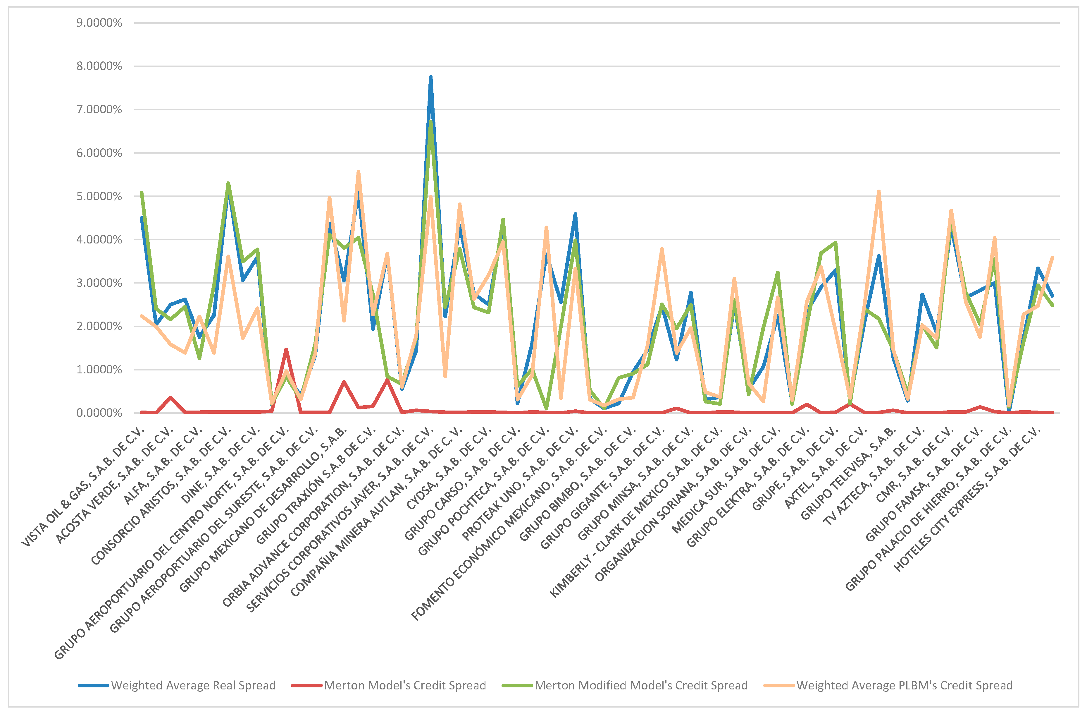
Figure 2.
Weighted Average Real Credit Spread vs. Merton Model, Merton Modified Model, and Weighted Average PLBM.
Figure 2.
Weighted Average Real Credit Spread vs. Merton Model, Merton Modified Model, and Weighted Average PLBM.
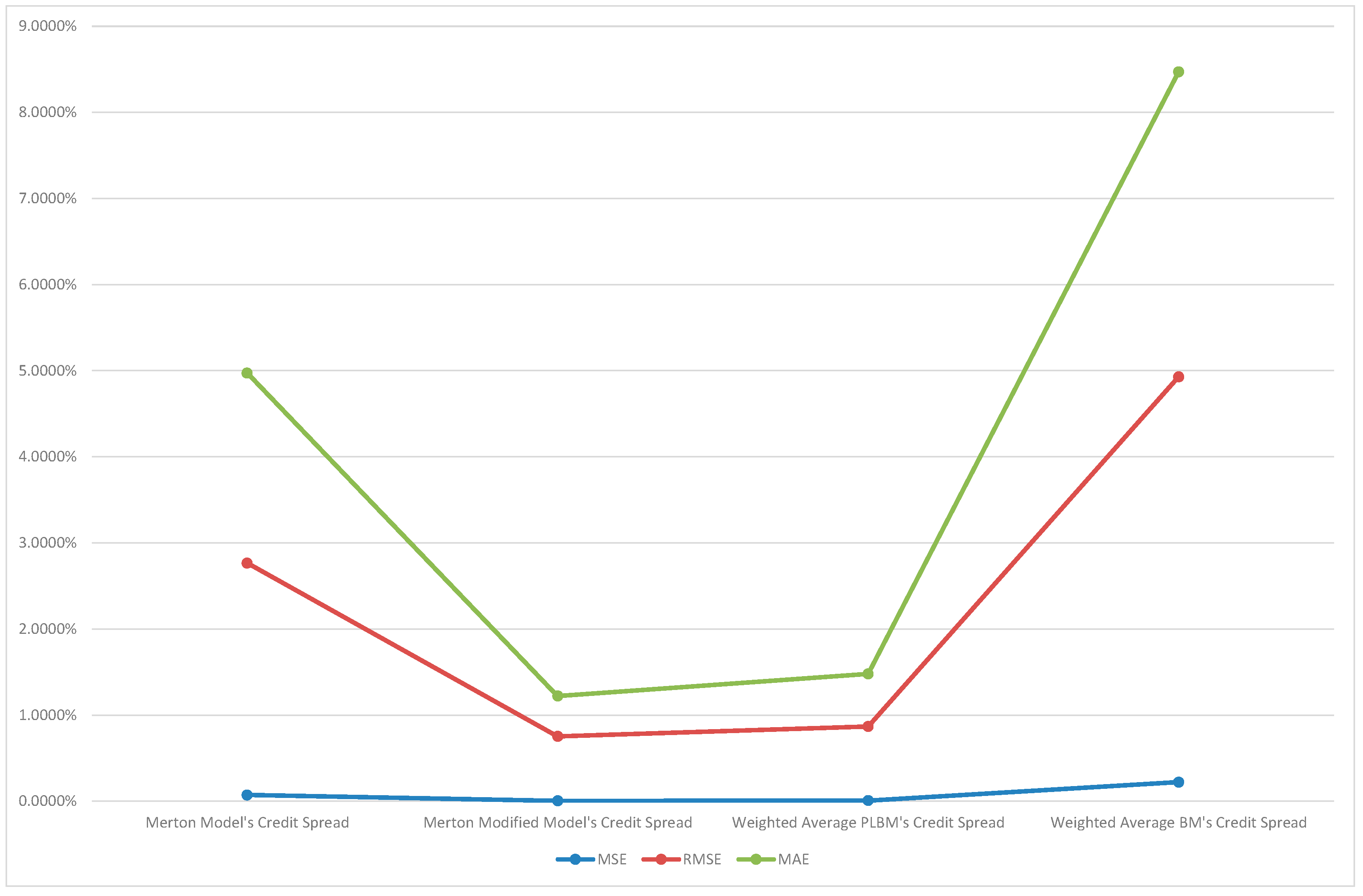
Figure 3.
Values of Companies’ Alphas.
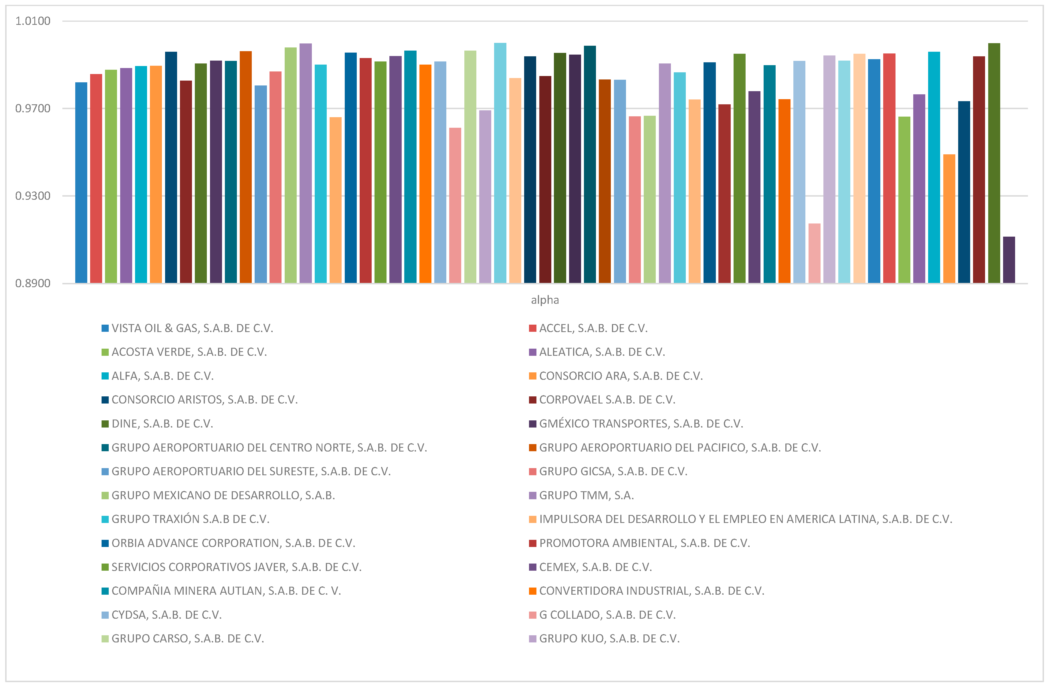

Table 1.
Companies analyzed by sector during 2022.
| Company | Sector | Currency | Total Amount of Debt | Weighted Average Duration | Number of Liabilities | Base Rate | Weighted Average Credit Spread | |
|---|---|---|---|---|---|---|---|---|
| VISTA OIL & GAS, S.A.B. DE C.V. | ENERGY | Mexican pesos | 374,433,035 | 1.56 | 1 | 1.29% | plus | 4.5000% |
| ACCEL, S.A.B. DE C.V. | INDUSTRIAL | Mexicano pesos | 778,951,000 | 5.66 | 3 | 1.29% | plus | 2.0373% |
| ACOSTA VERDE, S.A.B. DE C.V. | INDUSTRIAL | Mexican pesos | 3,056,401,729 | 7.34 | 17 | 4.63% | plus | 2.5000% |
| ALEATICA, S.A.B. DE C.V. | INDUSTRIAL | Mexican pesos | 6,317,721,000 | 5.57 | 1 | 1.29% | plus | 2.6223% |
| ALFA, S.A.B. DE C.V. | INDUSTRIAL | Mexican pesos | 50,000,000 | 2.36 | 1 | 4.,63% | plus | 1.7500% |
| CONSORCIO ARA, S.A.B. DE C.V. | INDUSTRIAL | Mexican pesos | 507,034,000 | 5.49 | 7 | 4.63% | plus | 2.2571% |
| CONSORCIO ARISTOS, S.A.B. DE C.V. | INDUSTRIAL | Mexican pesos | 62,160,150 | 4.89 | 7 | 4.63% | plus | 5.2459% |
| CORPOVAEL S.A.B. DE C.V. | INDUSTRIAL | Mexican pesos | 3,091,729,000 | 1.59 | 22 | 4.63% | plus | 3.0629% |
| DINE, S.A.B. DE C.V. | INDUSTRIAL | Mexican pesos | 210,000,000 | 2.08 | 1 | 4.63% | plus | 3.6000% |
| GMÉXICO TRANSPORTES, S.A.B. DE C.V. | INDUSTRIAL | Mexican pesos | 64,021,251 | 0.76 | 3 | 4.63% | plus | 0.2000% |
| GRUPO AEROPORTUARIO DEL CENTRO NORTE, S.A.B. DE C.V. | INDUSTRIAL | Mexican pesos | 2,700,000,000 | 1.91 | 3 | 4.63% | plus | 0.8937% |
| GRUPO AEROPORTUARIO DEL PACIFICO, S.A.B. DE C.V. | INDUSTRIAL | Mexican pesos | 13,800,000,000 | 2.88 | 6 | 4.63% | plus | 0.3896% |
| GRUPO AEROPORTUARIO DEL SURESTE, S.A.B. DE C.V. | INDUSTRIAL | Mexican pesos | 4,650,000 | 4.57 | 2 | 4.63% | plus | 1.3201% |
| GRUPO GICSA, S.A.B. DE C.V. | INDUSTRIAL | Mexican pesos | 4,429,347,000 | 4.70 | 6 | 4.63% | plus | 4.3734% |
| GRUPO MEXICANO DE DESARROLLO, S.A.B. | INDUSTRIAL | Mexican pesos | 65,973,515,000 | 1.46 | 5 | 4.63% | plus | 3.0532% |
| GRUPO TMM, S.A. | INDUSTRIAL | Mexican pesos | 80,000,000 | 0.53 | 5 | 4.63% | plus | 5.1000% |
| GRUPO TRAXIÓN S.A.B DE C.V. | INDUSTRIAL | Mexican pesos | 3,781,444,000 | 0.51 | 8 | 4.63% | plus | 1.9375% |
| IMPULSORA DEL DESARROLLO Y EL EMPLEO EN AMERICA LATINA, S.A.B. DE C.V. | INDUSTRIAL | Mexican pesos | 12,794,493,000 | 8.94 | 7 | 4.63% | plus | 3.6730% |
| ORBIA ADVANCE CORPORATION, S.A.B. DE C.V. | INDUSTRIAL | Mexican pesos | 985,533,730 | 0.50 | 1 | 4.63% | plus | 0.5500% |
| PROMOTORA AMBIENTAL, S.A.B. DE C.V. | INDUSTRIAL | Mexican pesos | 2,254,589,000 | 0.48 | 4 | 4.63% | plus | 1.4400% |
| SERVICIOS CORPORATIVOS JAVER, S.A.B. DE C.V. | INDUSTRIAL | Mexican pesos | 2,521,292,000 | 2.49 | 1 | 4.63% | plus | 7.7500% |
| CEMEX, S.A.B. DE C.V. | MATERIALS | Mexican pesos | 1,480,846,434 | 3.76 | 4 | 4.63% | plus | 2.2268% |
| COMPAÑIA MINERA AUTLAN, S.A.B. DE C. V. | MATERIALS | Mexican pesos | 2,806,123 | 5.29 | 4 | 4.63% | plus | 4.3163% |
| CONVERTIDORA INDUSTRIAL, S.A.B. DE C.V. | MATERIALS | Mexican pesos | 364,600,000 | 1.70 | 16 | 4.63% | plus | 2.7500% |
| CYDSA, S.A.B. DE C.V. | MATERIALS | Mexican pesos | 2,750,722,965 | 10.19 | 1 | 4.66% | plus | 2.5000% |
| G COLLADO, S.A.B. DE C.V. | MATERIALS | Mexican pesos | 173,649,000 | 0.11 | 1 | 4.63% | plus | 4.3633% |
| GRUPO CARSO, S.A.B. DE C.V. | MATERIALS | Mexican pesos | 3,500,000,000 | 2.25 | 1 | 4.63% | plus | 0.2150% |
| GRUPO KUO, S.A.B. DE C.V. | MATERIALS | Mexican pesos | 711,462,018 | 1.59 | 2 | 4.66% | plus | 1.5997% |
| GRUPO POCHTECA, S.A.B. DE C.V. | MATERIALS | Mexican pesos | 1,975,000,000 | 2.46 | 2 | 4.63% | plus | 3.6651% |
| MINERA FRISCO, S.A.B. DE C.V. | MATERIALS | Mexican pesos | 7,350,086,000 | 2.81 | 1 | 4.66% | plus | 2.5590% |
| PROTEAK UNO, S.A.B. DE C.V. | MATERIALS | Mexican pesos | 775,096,000 | 1.39 | 3 | 1.29% | plus | 4.5918% |
| ARCA CONTINENTAL | PRODUCTS OF FREQUENT CONSUMPTION | Mexican pesos | 12,296,941 | 3.23 | 9 | 4.65% | plus | 0.3239% |
| FOMENTO ECONÓMICO MEXICANO, S.A.B. DE C.V. | PRODUCTS OF FREQUENT CONSUMPTION | Mexican pesos | 5,662,000,000 | 3.47 | 3 | 4.63% | plus | 0.1066% |
| GRUMA, S.A.B. DE C.V. | PRODUCTS OF FREQUENT CONSUMPTION | Mexican pesos | 1,049,585,100 | 0.54 | 2 | 4.63% | plus | 0.2195% |
| GRUPO BIMBO, S.A.B. DE C.V. | PRODUCTS OF FREQUENT CONSUMPTION | Mexican pesos | 35,499,743,281 | 3.04 | 2 | 4.63% | plus | 0.9500% |
| GRUPO COMERCIAL CHEDRAUI, S.A.B. DE C.V. | PRODUCTS OF FREQUENT CONSUMPTION | Mexican pesos | 17,567,538,000 | 3.25 | 6 | 4.63% | plus | 1.4558% |
| GRUPO GIGANTE, S.A.B. DE C.V. | PRODUCTS OF FREQUENT CONSUMPTION | Mexican pesos | 8,968,888 | 4.86 | 6 | 4.63% | plus | 2.4681% |
| GRUPO HERDEZ, S.A.B. DE C.V. | PRODUCTS OF FREQUENT CONSUMPTION | Mexican pesos | 3,500,000,000 | 0.54 | 7 | 4.66% | plus | 1.2300% |
| GRUPO MINSA, S.A.B. DE C.V. | PRODUCTS OF FREQUENT CONSUMPTION | Mexican pesos | 99,903,500 | 2.15 | 7 | 4.63% | plus | 2.7737% |
| INDUSTRIAS BACHOCO, S.A.B. DE C.V. | PRODUCTS OF FREQUENT CONSUMPTION | Mexican pesos | 1,500,000,000 | 3.44 | 1 | 4.63% | plus | 0.3100% |
| KIMBERLY - CLARK DE MEXICO S.A.B. DE C.V. | PRODUCTS OF FREQUENT CONSUMPTION | Mexican pesos | 6,000,000,000 | 3.20 | 2 | 4.63% | plus | 0.3653% |
| ORGANIZACIÓN CULTIBA, S.A.B. DE CV | PRODUCTS OF FREQUENT CONSUMPTION | Mexican pesos | 751,670,000 | 2.95 | 6 | 4.63% | plus | 2.4913% |
| ORGANIZACION SORIANA, S.A.B. DE C.V. | PRODUCTS OF FREQUENT CONSUMPTION | Mexican pesos | 8,537,500,000 | 1.82 | 4 | 4.63% | plus | 0.5487% |
| GENOMMA LAB INTERNACIONAL, S.A.B. DE C.V. | HEALTH | Mexican pesos | 97,789,821,693 | 2.01 | 20 | 4.63% | plus | 1.0621% |
| MEDICA SUR, S.A.B. DE C.V. | HEALTH | Mexican pesos | 1,200,082,766 | 1.60 | 2 | 4.63% | plus | 2.2481% |
| EL PUERTO DE LIVERPOOL, S.A.B. DE C.V. | NON-COMMODITY GOODS AND SERVICES | Mexican pesos | 1,500,000,000 | 0.67 | 1 | 4.63% | plus | 0.2500% |
| GRUPO ELEKTRA, S.A.B. DE C.V. | NON-COMMODITY GOODS AND SERVICES | Mexican pesos | 13,079,861,000 | 0.75 | 10 | 4.63% | plus | 2.3412% |
| GRUPO VASCONIA S.A.B. | NON-COMMODITY GOODS AND SERVICES | Mexican pesos | 144,825,000 | 1.30 | 1 | 4.63% | plus | 2.9000% |
| GRUPE, S.A.B. DE C.V. | NON-COMMODITY GOODS AND SERVICES | Mexican pesos | 1,365,019,000 | 7.32 | 3 | 4.63% | plus | 3.2957% |
| AMERICA MOVIL, S.A.B. DE C.V. | TELECOMMUNICATIONS SERVICES | Mexican pesos | 34,080,000,000 | 0.51 | 10 | 4.93% | plus | 0.3151% |
| AXTEL, S.A.B. DE C.V. | TELECOMMUNICATIONS SERVICES | Mexican pesos | 3,204,745,000 | 5.50 | 2 | 4.63% | plus | 2.0958% |
| GRUPO RADIO CENTRO, S.A.B. DE C.V. | TELECOMMUNICATIONS SERVICES | Mexican pesos | 711,445,000 | 5.45 | 6 | 4.63% | plus | 3.6212% |
| GRUPO TELEVISA, S.A.B. | TELECOMMUNICATIONS SERVICES | Mexican pesos | 17,935,404,000 | 0.47 | 4 | 4.63% | plus | 1.2643% |
| MEGACABLE HOLDINGS, S.A.B. DE C.V. | TELECOMMUNICATIONS SERVICES | Mexican pesos | 6,823,407,000 | 0.58 | 4 | 4.63% | plus | 0.2800% |
| TV AZTECA, S.A.B. DE C.V. | TELECOMMUNICATIONS SERVICES | Mexican pesos | 5,708,000,000 | 3.22 | 4 | 4.63% | plus | 2.7405% |
| ALSEA, S.A.B. DE C.V. | NON-COMMODITY GOODS AND SERVICES | Mexican pesos | 564,645,163 | 1.95 | 2 | 4.63% | plus | 1.8474% |
| CMR, S.A.B. DE C.V. | NON-COMMODITY GOODS AND SERVICES | Mexican pesos | 1,141,234,000 | 3.33 | 1 | 4.63% | plus | 4.2975% |
| CORPORACION INTERAMERICANA DE ENTRETENIMIENTO, S.A.B. DE C.V. | NON-COMMODITY GOODS AND SERVICES | Mexican pesos | 850,000,000 | 0.31 | 4 | 4.63% | plus | 2.6559% |
| GRUPO FAMSA, S.A.B. DE C.V. | NON-COMMODITY GOODS AND SERVICES | Mexican pesos | 4,528,800,000 | 0.66 | 7 | 4.63% | plus | 2.8286% |
| GRUPO HOTELERO SANTA FE, S.A.B. DE C.V. | NON-COMMODITY GOODS AND SERVICES | Mexican pesos | 343,148,000 | 2.95 | 2 | 4.63% | plus | 3.0000% |
| GRUPO PALACIO DE HIERRO, S.A.B. DE C.V. | NON-COMMODITY GOODS AND SERVICES | Mexican pesos | 1,430,000 | 0.86 | 2 | 4.63% | plus | 0.0209% |
| GRUPO SPORTS WORLD, S.A.B. DE C.V. | NON-COMMODITY GOODS AND SERVICES | Mexican pesos | 1,789,362 | 0.76 | 2 | 4.63% | plus | 1.7221% |
| HOTELES CITY EXPRESS, S.A.B. DE C.V. | NON-COMMODITY GOODS AND SERVICES | Mexican pesos | 5,101,196,000 | 3.42 | 18 | 4.63% | plus | 3.3372% |
| NEMAK, S.A.B. DE C.V. | NON-COMMODITY GOODS AND SERVICES | Mexican pesos | 3,788,000,000 | 7.10 | 1 | 4.63% | plus | 2.7000% |
Table 2.
Analysis of DRSK, Bloomberg’s Credit Spread, and EDF of K.M.V. Moody’s.
| Company | DRSK 1 year | DRSK 2 years | Bloomberg Credit Spread | EDF 1 year | K.M.V. Moody's |
|---|---|---|---|---|---|
| VISTA OIL & GAS, S.A.B. DE C.V. | 0.224800% | 0.972400% | 2.46% | 3.02% | B1.edf |
| ACCEL, S.A.B. DE C.V. | 0.000000% | 0.000500% | 0.92% | 3.02% | B1.edf |
| ACOSTA VERDE, S.A.B. DE C.V. | 0.5221% | 1.4000% | 2.75% | 1.98% | Ba3.edf |
| ALEATICA, S.A.B. DE C.V. | 0.4825% | 2.1100% | 2.82% | 1.67% | Ba1.edf |
| ALFA, S.A.B. DE C.V. | 0.2673% | 0.9893% | 2.67% | 2.02% | Baa3.edf |
| CONSORCIO ARA, S.A.B. DE C.V. | 0.0260% | 0.2586% | 2.24% | 1.67% | Ba2.edf |
| CONSORCIO ARISTOS, S.A.B. DE C.V. | 1.5500% | 3.3800% | 3.15% | 35.00% | Caa-C.edf |
| CORPOVAEL S.A.B. DE C.V. | 1.6600% | 4.5500% | 3.27% | 7.58% | B3.edf |
| DINE, S.A.B. DE C.V. | 0.0000% | 0.0003% | 0.71% | 3.02% | B1.edf |
| GMÉXICO TRANSPORTES, S.A.B. DE C.V. | 0.7874% | 2.3300% | 2.76% | 3.02% | B1.edf |
| GRUPO AEROPORTUARIO DEL CENTRO NORTE, S.A.B. DE C.V. | 0.0012% | 0.0504% | 1.47% | 6.71% | B3.edf |
| GRUPO AEROPORTUARIO DEL PACIFICO, S.A.B. DE C.V. | 0.0120% | 0.1699% | 1.83% | 0.37% | Baa1.edf |
| GRUPO AEROPORTUARIO DEL SURESTE, S.A.B. DE C.V. | 0.0008% | 0.0376% | 1.56% | 6.71% | B3.edf |
| GRUPO GICSA, S.A.B. DE C.V. | 3.7100% | 5.9300% | 3.31% | 1.67% | Ba2.edf |
| GRUPO MEXICANO DE DESARROLLO, S.A.B. | 0.3472% | 1.1600% | 2.55% | 3.02% | B2.edf |
| GRUPO TMM, S.A. | 0.5808% | 1.9000% | 2.56% | 6.71% | B3.edf |
| GRUPO TRAXIÓN S.A.B DE C.V. | 0.2951% | 1.1800% | 2.38% | 3.02% | B1.edf |
| IMPULSORA DEL DESARROLLO Y EL EMPLEO EN AMERICA LATINA, S.A.B. DE C.V. | 0.0045% | 0.1157% | 1.66% | 4.35% | B2.edf |
| ORBIA ADVANCE CORPORATION, S.A.B. DE C.V. | 0.2143% | 0.8712% | 2.39% | 0.98% | Ba1.edf |
| PROMOTORA AMBIENTAL, S.A.B. DE C.V. | 0.0006% | 0.0262% | 1.37% | 1.67% | Ba2.edf |
| SERVICIOS CORPORATIVOS JAVER, S.A.B. DE C.V. | 0.0000% | 0.0000% | 0.39% | 35.00% | Caa-C.edf |
| CEMEX, S.A.B. DE C.V. | 0.5300% | 1.7500% | 2.71% | 0.93% | Ba1.edf |
| COMPAÑIA MINERA AUTLAN, S.A.B. DE C. V. | 0.0057% | 0.1013% | 1.87% | 6.71% | B3.edf |
| CONVERTIDORA INDUSTRIAL, S.A.B. DE C.V. | 0.0000% | 0.0003% | 0.74% | 0.37% | Baa1.edf |
| CYDSA, S.A.B. DE C.V. | 0.0127% | 0.1903% | 2.17% | 3.52% | Ba2.edf |
| G COLLADO, S.A.B. DE C.V. | 0.0426% | 0.3397% | 2.33% | 6.71% | B3.edf |
| GRUPO CARSO, S.A.B. DE C.V. | 0.0325% | 0.3485% | 2.20% | 0.37% | Baa1.edf |
| GRUPO KUO, S.A.B. DE C.V. | 0.0001% | 0.0147% | 1.41% | 0.98% | Ba1.edf |
| GRUPO POCHTECA, S.A.B. DE C.V. | 0.0140% | 0.1857% | 1.79% | 3.02% | B3.edf |
| MINERA FRISCO, S.A.B. DE C.V. | 0.3140% | 1.1300% | 2.48% | 0.37% | Baa1.edf |
| PROTEAK UNO, S.A.B. DE C.V. | 0.9781% | 2.7900% | 2.69% | 6.71% | B3.edf |
| ARCA CONTINENTAL | 0.0005% | 0.0292% | 1.66% | 0.37% | Baa1.edf |
| FOMENTO ECONÓMICO MEXICANO, S.A.B. DE C.V. | 0.0001% | 0.0133% | 1.42% | 0.37% | Baa1.edf |
| GRUMA, S.A.B. DE C.V. | 0.0330% | 0.3536% | 2.39% | 0.37% | Baa1.edf |
| GRUPO BIMBO, S.A.B. DE C.V. | 0.0270% | 0.2851% | 2.34% | 0.38% | Baa2.edf |
| GRUPO COMERCIAL CHEDRAUI, S.A.B. DE C.V. | 0.0131% | 0.1813% | 2.18% | 6.71% | B3.edf |
| GRUPO GIGANTE, S.A.B. DE C.V. | 0.0011% | 0.0505% | 1.60% | 3.02% | B1.edf |
| GRUPO HERDEZ, S.A.B. DE C.V. | 0.1376% | 0.7592% | 2.71% | 4.35% | B2.edf |
| GRUPO MINSA, S.A.B. DE C.V. | 0.0005% | 0.0444% | 1.57% | 1.98% | Ba3.edf |
| INDUSTRIAS BACHOCO, S.A.B. DE C.V. | 0.0001% | 0.0141% | 1.42% | 0.37% | Baa1.edf |
| KIMBERLY - CLARK DE MEXICO S.A.B. DE C.V. | 0.0000% | 0.0030% | 1.08% | 0.37% | Baa1.edf |
| ORGANIZACIÓN CULTIBA, S.A.B. DE CV | 0.0006% | 0.0671% | 1.62% | 0.37% | Baa1.edf |
| ORGANIZACION SORIANA, S.A.B. DE C.V. | 0.0029% | 0.0814% | 1.86% | 0.98% | Ba1.edf |
| GENOMMA LAB INTERNACIONAL, S.A.B. DE C.V. | 0.0431% | 0.3651% | 2.23% | 3.02% | B1.edf |
| MEDICA SUR, S.A.B. DE C.V. | 0.4348% | 1.7100% | 2.78% | 4.35% | B2.edf |
| EL PUERTO DE LIVERPOOL, S.A.B. DE C.V. | 0.0000% | 0.0040% | 1.06% | 0.37% | Baa1.edf |
| GRUPO ELEKTRA, S.A.B. DE C.V. | 0.0031% | 0.1278% | 1.50% | 3.02% | B1.edf |
| GRUPO VASCONIA S.A.B. | 2.4100% | 4.4300% | 3.21% | 3.02% | B1.edf |
| GRUPE, S.A.B. DE C.V. | 0.0000% | 0.0000% | 0.42% | 1.98% | Ba3.edf |
| AMERICA MOVIL, S.A.B. DE C.V. | 0.0133% | 0.1824% | 1.49% | 0.48% | Baa2.edf |
| AXTEL, S.A.B. DE C.V. | 3.7300% | 6.5100% | 2.50% | 4.35% | B2.edf |
| GRUPO RADIO CENTRO, S.A.B. DE C.V. | 0.0000% | 0.0000% | 0.28% | 6.71% | B3.edf |
| GRUPO TELEVISA, S.A.B. | 0.6507% | 2.2900% | 1.99% | 1.98% | Ba3.edf |
| MEGACABLE HOLDINGS, S.A.B. DE C.V. | 0.0072% | 0.1325% | 1.32% | 0.37% | Baa1.edf |
| TV AZTECA, S.A.B. DE C.V. | 4.0800% | 5.7600% | 2.50% | 35.00% | Caa-C.edf |
| ALSEA, S.A.B. DE C.V. | 0.1980% | 0.8646% | 2.70% | 3.02% | B1.edf |
| CMR, S.A.B. DE C.V. | 1.8000% | 3.0600% | 3.13% | 2.02% | Baa3.edf |
| CORPORACION INTERAMERICANA DE ENTRETENIMIENTO, S.A.B. DE C.V. | 0.0000% | 0.0032% | 0.91% | 3.02% | Baa3.edf |
| GRUPO FAMSA, S.A.B. DE C.V. | 14.3000% | 16.0700% | 4.10% | 35.00% | Caa-C.edf |
| GRUPO HOTELERO SANTA FE, S.A.B. DE C.V. | 0.0378% | 0.3362% | 2.23% | 3.02% | B1.edf |
| GRUPO PALACIO DE HIERRO, S.A.B. DE C.V. | 0.0000% | 0.0000% | 0.38% | 0.37% | Baa1.edf |
| GRUPO SPORTS WORLD, S.A.B. DE C.V. | 7.5300% | 10.5500% | 3.57% | 3.20% | B1.edf |
| HOTELES CITY EXPRESS, S.A.B. DE C.V. | 0.5782% | 2.1200% | 2.89% | 6.71% | B3.edf |
| NEMAK, S.A.B. DE C.V. | 0.2963% | 1.0000% | 2.68% | 3.20% | B1.edf |
| MAX BLOOMBERG Y MOODY'S ( FAMSA) | 14.300% | 16.070% | 4.100% | 35.000% | |
| MIN BLOOMBERG Y MOODY'S (PALACIO DE HIERRO) | 0.000% | 0.000% | 0.280% | 0.370% | |
| AVERAGE | 0.765% | 1.433% | 2.052% | 4.777% | |
| CORRELATION BETWEEN DRSK 1 YEAR VS.EDF I YEAR | 51% | ||||
| CORRELATION BETWEEN EDF 1 YEAR AND DEBT COST CALCULATED BY BLOOMBERG | 55% | ||||
| CORRELATION BETWEEN DRSK 1 YEAR AND DEBT COST CALCULATED BY BLOOMBERG | 20% |
Table 3.
Results of the models applying the value of the fit parameter G.
| Bloomberg | Merton | BM | PLBM | Modified Merton |
|
|---|---|---|---|---|---|
| G Value | -0.174 | -2.16 | -13.105 | 0.504 | 0.767 |
Table 4.
Market Value of Company.
| Market Value of Equity multiplied by the proportion of debts referenced to a base rate. | Merton's Modified Model Value of Firm | Traditional Merton's Model Value of Firm | |
|---|---|---|---|
| VISTA OIL & GAS, S.A.B. DE C.V. | 3,204,369,379 | 4,094,440,938 | 4,108,397,401 |
| ACCEL, S.A.B. DE C.V. | 70,795,633 | 1,515,398,832 | 1,510,882,175 |
| ACOSTA VERDE, S.A.B. DE C.V. | 4,174,491,988 | 5,359,702,736 | 5,390,721,949 |
| ALEATICA, S.A.B. DE C.V. | 4,412,626,304 | 19,198,159,763 | 18,777,304,633 |
| ALFA, S.A.B. DE C.V. | 16,888,265 | 82,834,452 | 75,975,063 |
| CONSORCIO ARA, S.A.B. DE C.V. | 376,566,920 | 1,215,757,837 | 1,463,895,025 |
| CONSORCIO ARISTOS, S.A.B. DE C.V. | 336,223,889 | 647,612,247 | 565,460,656 |
| CORPOVAEL S.A.B. DE C.V. | 5,621,705,400 | 10,211,457,528 | 10,024,864,591 |
| DINE, S.A.B. DE C.V. | 366,936,262 | 681,112,143 | 685,448,591 |
| GMÉXICO TRANSPORTES, S.A.B. DE C.V. | 9,573,368 | 86,825,181 | 86,468,867 |
| GRUPO AEROPORTUARIO DEL CENTRO NORTE, S.A.B. DE C.V. | 1,084,426,658 | 4,713,813,946 | 4,679,892,238 |
| GRUPO AEROPORTUARIO DEL PACIFICO, S.A.B. DE C.V. | 52,297,228,499 | 91,120,045,883 | 90,885,409,863 |
| GRUPO AEROPORTUARIO DEL SURESTE, S.A.B. DE C.V. | 27,154,255 | 50,608,933 | 50,682,460 |
| GRUPO GICSA, S.A.B. DE C.V. | 2,307,649,642 | 14,836,771,752 | 14,590,502,079 |
| GRUPO MEXICANO DE DESARROLLO, S.A.B. | 659,782,574 | 85,512,291,351 | 79,304,549,758 |
| GRUPO TMM, S.A. | 11,962,738 | 149,367,099 | 119,400,933 |
| GRUPO TRAXIÓN S.A.B DE C.V. | 6,750,049,962 | 16,585,294,238 | 12,408,855,277 |
| IMPULSORA DEL DESARROLLO Y EL EMPLEO EN AMERICA LATINA, S.A.B. DE C.V. | 74,218,739,600 | 210,947,833,546 | 202,277,465,837 |
| ORBIA ADVANCE CORPORATION, S.A.B. DE C.V. | 13,675,282,346 | 15,380,978,496 | 15,391,528,072 |
| PROMOTORA AMBIENTAL, S.A.B. DE C.V. | 1,012,278,749 | 3,884,407,934 | 3,664,320,211 |
| SERVICIOS CORPORATIVOS JAVER, S.A.B. DE C.V. | 1,663,862,470 | 5,510,378,938 | 5,572,151,511 |
| CEMEX, S.A.B. DE C.V. | 9,573,046,550 | 17,441,427,463 | 17,412,842,226 |
| COMPAÑIA MINERA AUTLAN, S.A.B. DE C. V. | 194,162,679 | 16,021,317,720 | 332,679,524 |
| CONVERTIDORA INDUSTRIAL, S.A.B. DE C.V. | 90,424,438 | 511,035,949 | 511,617,569 |
| CYDSA, S.A.B. DE C.V. | 1,262,474,450 | 12,890,929,557 | 12,522,098,956 |
| G COLLADO, S.A.B. DE C.V. | 993,957,189 | 1,178,758,084 | 1,179,043,858 |
| GRUPO CARSO, S.A.B. DE C.V. | 7,265,439,986 | 16,021,317,720 | 16,021,317,720 |
| GRUPO KUO, S.A.B. DE C.V. | 210,958,856 | 1,364,007,530 | 1,218,098,575 |
| GRUPO POCHTECA, S.A.B. DE C.V. | 145,109,485 | 19,001,717,935 | 2,778,199,366 |
| MINERA FRISCO, S.A.B. DE C.V. | 5,218,340,679 | 17,726,200,951 | 17,425,021,074 |
| PROTEAK UNO, S.A.B. DE C.V. | 1,630,292,378 | 3,080,664,077 | 2,977,257,083 |
| ARCA CONTINENTAL | 25,948,655 | 53,678,868 | 52,858,416 |
| FOMENTO ECONÓMICO MEXICANO, S.A.B. DE C.V. | 4,845,019,144 | 14,962,279,256 | 14,694,998,128 |
| GRUMA, S.A.B. DE C.V. | 36,743,809,015 | 39,699,333,879 | 39,706,627,231 |
| GRUPO BIMBO, S.A.B. DE C.V. | 41,978,149,087 | 106,304,630,890 | 102,354,542,194 |
| GRUPO COMERCIAL CHEDRAUI, S.A.B. DE C.V. | 6,614,018,439 | 34,076,733,248 | 34,134,335,048 |
| GRUPO GIGANTE, S.A.B. DE C.V. | 9,928,029 | 30,357,513 | 30,526,314 |
| GRUPO HERDEZ, S.A.B. DE C.V. | 5,976,931,305 | 12,087,429,492 | 10,722,916,842 |
| GRUPO MINSA, S.A.B. DE C.V. | 173,333,533 | 328,648,774 | 321,952,993 |
| INDUSTRIAS BACHOCO, S.A.B. DE C.V. | 3,695,120,296 | 7,325,738,731 | 7,349,128,005 |
| KIMBERLY - CLARK DE MEXICO S.A.B. DE C.V. | 13,287,374,553 | 36,864,413,917 | 28,910,749,020 |
| ORGANIZACIÓN CULTIBA, S.A.B. DE CV | 389,146,248 | 1,575,794,781 | 1,563,252,455 |
| ORGANIZACION SORIANA, S.A.B. DE C.V. | 1,553,836,356 | 12,284,054,074 | 11,843,481,628 |
| GENOMMA LAB INTERNACIONAL, S.A.B. DE C.V. | 11,525,792,193 | 21,166,453,135 | 20,833,698,941 |
| MEDICA SUR, S.A.B. DE C.V. | 3,135,268,077 | 4,942,545,502 | 4,873,866,279 |
| EL PUERTO DE LIVERPOOL, S.A.B. DE C.V. | 1,750,533,577 | 3,497,437,585 | 3,497,560,759 |
| GRUPO ELEKTRA, S.A.B. DE C.V. | 14,129,648,854 | 28,042,057,105 | 28,060,114,726 |
| GRUPO VASCONIA S.A.B. | 119,639,220 | 307,458,765 | 303,848,523 |
| GRUPE, S.A.B. DE C.V. | 874,786,166 | 4,191,961,636 | 3,827,468,979 |
| AXTEL, S.A.B. DE C.V. | 2,605,355,905 | 12,246,999,368 | 12,106,684,412 |
| GRUPO RADIO CENTRO, S.A.B. DE C.V. | 303,409,575 | 2,223,974,452 | 1,982,372,196 |
| GRUPO TELEVISA, S.A.B. | 9,937,231,783 | 29,043,072,558 | 30,864,849,971 |
| MEGACABLE HOLDINGS, S.A.B. DE C.V. | 43,799,145,112 | 53,770,289,727 | 53,756,011,475 |
| TV AZTECA, S.A.B. DE C.V. | 2,175,351 | 7,853,857,310 | 7,864,508,956 |
| ALSEA, S.A.B. DE C.V. | 236,297,064 | 909,368,794 | 966,182,735 |
| CMR, S.A.B. DE C.V. | 342,786,454 | 1,899,382,295 | 1,783,612,196 |
| CORPORACION INTERAMERICANA DE ENTRETENIMIENTO, S.A.B. DE C.V. | 730,475,438 | 1,629,356,797 | 1,628,826,733 |
| GRUPO FAMSA, S.A.B. DE C.V. | 137,096,822 | 9,160,107,202 | 6,937,247,893 |
| GRUPO HOTELERO SANTA FE, S.A.B. DE C.V. | 210,334,518 | 1,117,108,020 | 919,304,660 |
| GRUPO PALACIO DE HIERRO, S.A.B. DE C.V. | 1,095,540 | 2,739,388 | 2,728,061 |
| GRUPO SPORTS WORLD, S.A.B. DE C.V. | 9,626,767 | 13,643,775 | 12,575,700 |
| HOTELES CITY EXPRESS, S.A.B. DE C.V. | 1,382,992,127 | 10,005,621,965 | 9,696,004,717 |
| NEMAK, S.A.B. DE C.V. | 1,067,967,384 | 7,028,423,000 | 8,060,551,072 |
Disclaimer/Publisher’s Note: The statements, opinions and data contained in all publications are solely those of the individual author(s) and contributor(s) and not of MDPI and/or the editor(s). MDPI and/or the editor(s) disclaim responsibility for any injury to people or property resulting from any ideas, methods, instructions or products referred to in the content. |
© 2023 by the authors. Licensee MDPI, Basel, Switzerland. This article is an open access article distributed under the terms and conditions of the Creative Commons Attribution (CC BY) license (http://creativecommons.org/licenses/by/4.0/).
Copyright: This open access article is published under a Creative Commons CC BY 4.0 license, which permit the free download, distribution, and reuse, provided that the author and preprint are cited in any reuse.


