1. Introduction
There are various complex systems in the fields of natural science and social science, such as atmospheric systems, computer networks, human societies and so on [
1,
2,
3,
4]. In these complex systems, there are numerous system factors, which are interrelated and work together on the operating state or output result of the system. But there is no doubt that among all these factors, there are often few that play a dominant role, which we call the key influencing factors of the complex system [
5,
6]. In complex systems constrained by multiple factors, it is of great significance to identify the key influencing factors for mastering the evolution and development law of the system and obtaining scientific decision-making suggestions or schemes [
7].
In fact, in order to identify the key influencing factors in a complex system, we need a deep knowledge and understanding of the system itself. On the one hand, it requires long-term observation of the system; on the other hand, it requires the use of advanced technologies and methods to conduct scientific analysis of the system. As a kind of science, causal inference already affects important aspects of everyday life, and has the potential to expand its reach even further, covering the exploration and solution of major problems, from the development of new drugs to economic policymaking, from education and machine technology to gun control and even global warming [
8,
9,
10]. It can also be used to model and explore the complex system problems [
11].
In this paper, in order to identify the key influencing factors in complex systems, we propose a model based on heuristic causal inference, which consists of three main modules: causal network learning, heuristic causal effect calculation, and key influencing factors identification. Causal network learning enables us to re-understand the concerned system from the perspective of causation, heuristic causal effect calculation enables us to analyze the interaction between system variables quantitatively, and key influencing factors identification enables us to grasp the core joints of the system accurately. Based on the observation dataset, we confirm the validity of the proposed method.
The novel contributions of our work are summarized as follows:
(1) Proposing the idea of using causal inference to identify the key influencing factors of some complex systems. We examine complex systems from another perspective of causality, which is different from the traditional simulation or qualitative analysis methods.
(2) Proposing a causal network learning method combining prior knowledge. Observation datasets of complex systems often belong to high dimensional and heterogeneous dataset, and it is difficult for traditional methods to learn causal network from these datasets directly. Combined with prior knowledge, we got the causal network wanted and reduced the computational complexity effectively.
(3) Proposing a heuristic causal effect calculation method to identify the key influencing factors of some complex systems. Inspired by the relevant ideas of network science, we defined the concepts of causal path length and causal path contribution degree, and proposed a heuristic causal effect calculation method. Depending on the size of the causal effect, the key influencing factors in the complex system can be identified effectively.
The rest of this paper is organized as follows: the second section briefly introduces the relevant work, the third section introduces the overall structure of the proposed model and the detailed technical method, the fourth section describes the process and results of the experiment, the fifth section analyzes the experimental results, and the sixth section summarizes the content of the paper and looks forward to the next steps.
2. Related Work
Researchers are always interested in exploring kinds of complex systems. There are two main methods to identify the key influencing factors of complex systems: experimental simulation method and Decision Trial and Evaluation Laboratory method (DEMATEL) [
12,
13,
14]. Among them, the experimental simulation method is mainly used in natural science, which is based on positivism. DEMATEL is mainly used in social science. It uses the methods of investigation, qualitative analysis and quantitative calculation to identify the key influencing factors of systemic problems in social activities.
2.1. Experimental Simulation Method
In the field of natural science, experimental simulation method constructs a system simulation model around the target problem, and statistically analyze the influence degree of multiple factors on the system by means of variable control, etc. On this basis, key influencing factors of the system can be identified. In 2021, Rong et al. [
15] established the mathematical model of key components of the cross-delivery system of launch vehicle. On this basis, the system simulation model was constructed by using professional software tools, and the key influencing factors of the cross-delivery system were identified through modeling and simulation. In 2020, Zhang et al. [
16] studied the static characteristics of double-cable suspension bridges based on the finite element analysis model, found out the key design parameters by calculating the effects of various parameters on the mechanical performance of the bridge, and put forward some specific suggestions for the design of such bridges. In 2013,Chen et al. [
17] analyzed the influence of four factors in the space electronic equipment on the spectrum distribution of sound signals through single factor experiment, and identified the key influencing factors by orthogonal test method, which provided guidance for further identification of excess residues in the system. In 2021,Sun et al. [
18] established a relevant chemical potential gradient model for MAP crystal growth, identified four key influencing factors, and quantitatively analyzed their effects on the growth rate of MAP crystal, providing basis and guidance for scientific regulation of MAP crystallization process in industrial practice.
2.2. Factual Decision Trial and Evaluation Laboratory Method (DEMATEL)
In the field of social science, in the 1970s, American scholars Fontela and Gabus [
19,
20,
21] created Factual Decision Trial and Evaluation Laboratory Method (DEMATEL), which based on graph theory and matrix theory, conducted a comprehensive analysis of the internal correlation between multiple influencing factors of complex systems. It is widely used in systems engineering, management science and many other fields. In practical application, the method is deeply integrated with other methods, and has been continuously improved and expanded [
22,
23,
24,
25,
26,
27,
28].
In 2021, aiming at the identification of key influencing factors affecting the user experience of mobile reading APPs, Zhang et al. [
22] established a fuzzy DEMATEL model by introducing triangular fuzzy numbers and extending the single value of the comparison matrix to the fuzzy interval, and provided a suitable judgment space for decision makers. It effectively solved the defects of the traditional DEMATEL method that the subjective deviation of expert judgment is large, and it is difficult to be directly expressed by accurate numbers. In 2022, Li et al. [
23] constructed an evaluation index system in view of the institutional obstacles faced by China’s integration innovation, used AHP-DEMATEL method to conduct an empirical analysis of this problem, identified key institutional obstacles such as confidentiality system and intellectual property system, and provided countermeasures and suggestions for decision-makers to carry out reform and innovation. In 2022, aiming at the problem of risk identification and control in enterprise product development, Chui et al. [
24] combined network analysis with DEMATEL, established ANP-DEMATEL model, studied the causal relationship between various risk factors and their relative importance, and identified six key influencing factors in the process of product development. In view of the important theoretical significance and application value of DEMATEL method in the study of complex systems, Sun et al. [
19,
21] conducted a comprehensive study on DEMATEL method from multiple perspectives, such as basic theory, operation logic and cross-integration with other methods, systematically reviewed the research status and development trends of the method. It provides reference and guidance for the subsequent theoretical research and practical application.
In general, the above two methods have their own characteristics, but also have their own limitations and shortcomings. The method based on experimental simulation has the characteristics of positivism, but it needs to establish a system simulation model, which is often difficult to achieve for complex giant systems. DEMATEL method pays attention to the analysis of the correlation between various influencing factors of complex systems and tries to grasp the operation law of the system as a whole. However, its evaluation scale and determination of the self-dependence relationship between factors are greatly affected by subjective factors, and this method generally requires extensive research, which takes a long time and is more difficult.
With the construction and improvement of big data environment in all walks of life, the evolution law of various complex systems is expected to be revealed through data science. At the same time, in recent years, the relevant methods of causal science have aroused great interest of scholars. Combining causal method with observational data to reveal the nature of things has become a hot topic at present. In view of this, a heuristic causal inference method was proposed to solve the problem of difficult identification of key influencing factors in complex systems. Experiment on semiconductor manufacturing datasets was carried out to verify the effectiveness of the method. Compared with the experimental simulation and DEMATEL method, the method proposed in this paper is more adaptable and feasible with the support of observation data.
3. Proposed Method
According to the basic assumption of DEMATEL’s method, suppose a system has influencing factors, denoted as, there is a mutual influence relationship between these factors, and this relationship can be expressed in the form of a matrix. The initial direct influence matrix is constructed as, where is the degree of direct influence of the factor on, and.
In practical studies, it is common to focus on how one factor in the system is affected by other factors. Let be the target variable that the researcher is interested in, is other system factors related to the target variable, and the influence degree of on the target variable is recorded as, is the direct influence degree of the factor on the target variable.
In descending order according to the value of, the higher the ranking, the greater the influence of the corresponding system factors on the target variables. According to this idea, several key influencing factors of the complex system can be determined.
3.1. Technical Framework
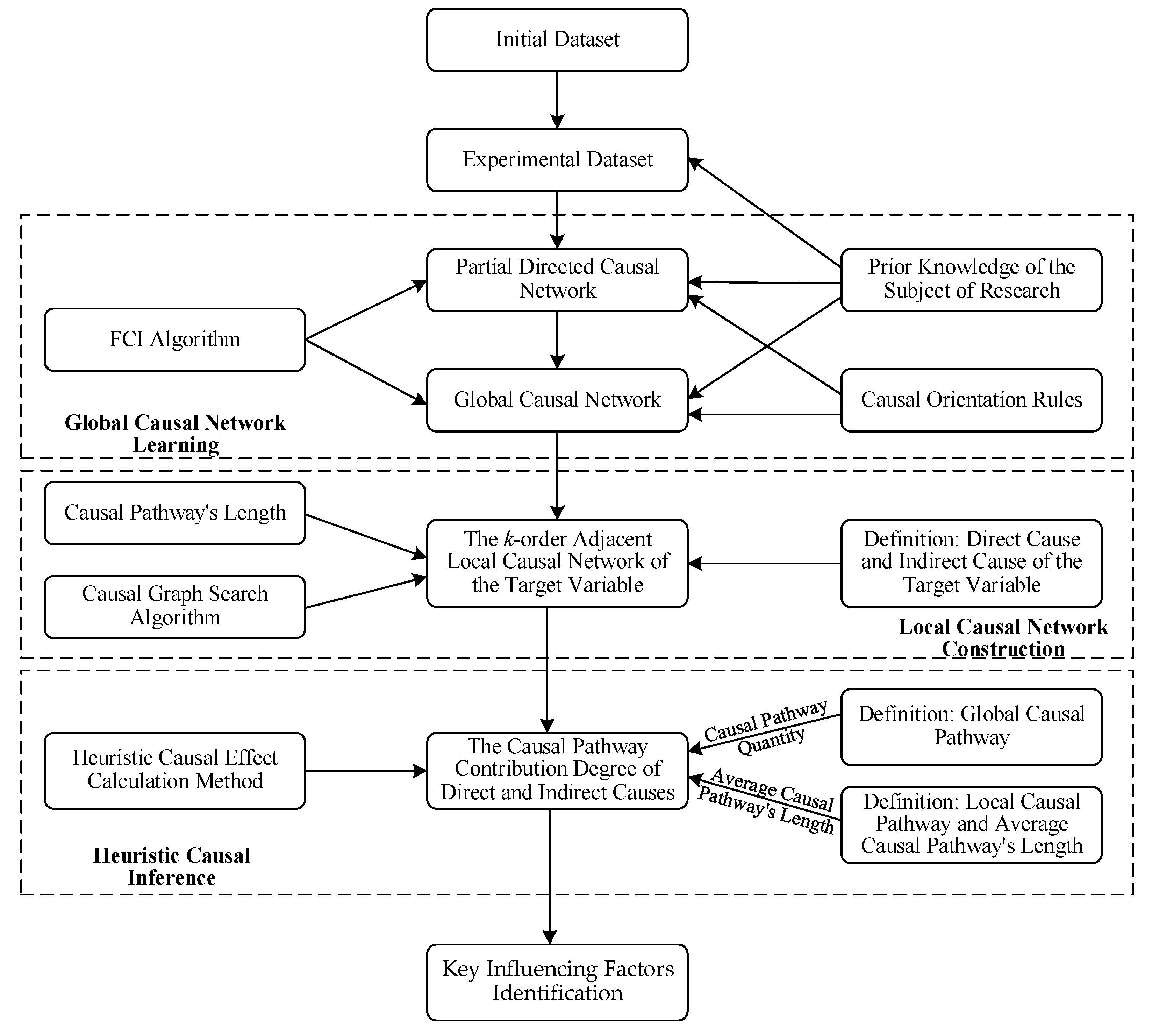
The essence of identification of the key influencing factors is to clarify the complex and nonlinear relationship among the factors in the complex system. With the support of an observation dataset, we adopt the methods of causal discovery and heuristic causal inference to solve the above problem. The overall technical framework of the research is shown in
Figure 1.
In the above model, the key steps involved are causal network learning and heuristic causal inference. Among them, causal network learning is carried out in the way of first global and then local. In the global network learning stage, the FCI algorithm [
29,
30] is used to acquire the initial network, and the supplementary orientation of the initial network is combined with prior knowledge. In the stage of local network learning, the adjacent local causal network of target variables is defined in combination with the Markov blanket [
31]. Heuristic causal inference mainly calculates the causal path contribution degree of each cause variable (direct cause and indirect cause) in the local causal network to the target variable, to replace the causal effect of the cause variable on the target variable. According to the above ideas, the correlation between various factors in the system can be revealed quantitatively, and several key influencing factors with greater causal influence on the target variables can be determined to provide basis and guidance for system regulation.
3.2. Causal Network Learning
In data science, the evolution and development of a system can be revealed through data analysis. In this section, we take the observed data as input, and use the FCI algorithm combined with prior knowledge to learn the global causal network behind the data. On this basis, the method of network search is used to obtain the local causal network around the selected target variable. The aim is to provide a trusted network structure for heuristic causal inference in the next section.
3.2.1. Global Causal Network Learning
Let be a dimensional set of variables in a given system, where, is the selected target variable and is the cause variables associated with. Let be the group observation datasets of, and now it is necessary to discover the causal relationship between variables in based on the observation datasets. We use the FCI algorithm to learn the initial causal network among variables, combined with prior knowledge to supplement the orientation. Finally, we get the global causal network. The basic steps are as follows:
Step 1: Use algorithm 4.1 in [
32] to learn the causal skeleton (
) between variables of the researched system, meanwhile, obtain the separate set (
) and the unmasked triplet (
).
Step 2: Use algorithm 4.2 in [
32] to conduct orientation of V-structure in
and update it.
Step 3: Use algorithm 4.3 in [
32] to obtain the final causal skeleton, update it and update the separate set (
).
Step 4: Use algorithm 4.2 in [
32] to conduct orientation of the V-structure in
and update it again.
Step 5: Apply rules (R1) ~ (R10) in [
33] to conduct causal orientation of skeleton (
) as much as possible, and then update it.
Step 6: Use prior knowledge to conduct supplementary orientation for and obtain the global causal network
In the above causal discovery process, the hypothesis to be satisfied include:
Causal Sufficiency Hypothesis: The variable set is causally sufficient when the direct cause variables of any two variables of are also included in itself.
Causal Markov Hypothesis: For a set of variables that satisfy the causal sufficiency hypothesis, the set of variables satisfies the causal Markov hypothesis if every variable is mutually independent of its non-descendant nodes, in the condition of given its causal parent nodes.
Causal Loyalty Hypothesis: If variables and are independent or conditionally independent under the premise of a given variable set, then in the causal network composed of variables and their causal dependency relationships, all pathways between and are d-separated by the appropriate variable in.Then the joint distribution of all random variables in is said to be causal loyalty to the network
3.2.2. Local Causal Network Construction
In order to identify the factors that have key impact on the target, it is natural to search the local causal network of the target. The Markov blanket is the most typical one. For the convenience of description, the following definition is given first:
Definition 1: Causal Operation Criterion - For causal variables A and B, it is supposed that the experimenter can manipulate variable A by setting its value to, denoted as.If the experimenter observes that for some and (within the time window), it indicates that is the cause of (within).
Definition 2: Direct and Indirect Cause - If is the cause of according to definition 1, then is an indirect cause of with respect to a set, if and only if some assignment of to (by operation) is not a cause of, otherwise is a direct cause of.
According to the above definitions, for the target variable,some variables in the global causal network are its direct causes and others are its indirect causes. Combined with Markov blanket, the adjacent local causal network of the target variable can be constructed as follows:
Step 1: Choose the target variable and obtain its Markov blanket.
Step 2: Determine the order of the adjacent local causal network.
Step 3: Starting from the target variable, search its direct and indirect causes within steps. Among them, the pathway length between the target and its direct cause is defined as 1, and so on.
Step 4: Take the target variable and its direct and indirect causes found in Step 3 as nodes, along with the edges between them, to build the local causal network.
3.3. Heuristic Causal Inference
With the global and local causal networks obtained in the above section as inputs, a heuristic causal inference method is designed to quantitatively calculate the causal path contribution degree of cause variables to the target variable.
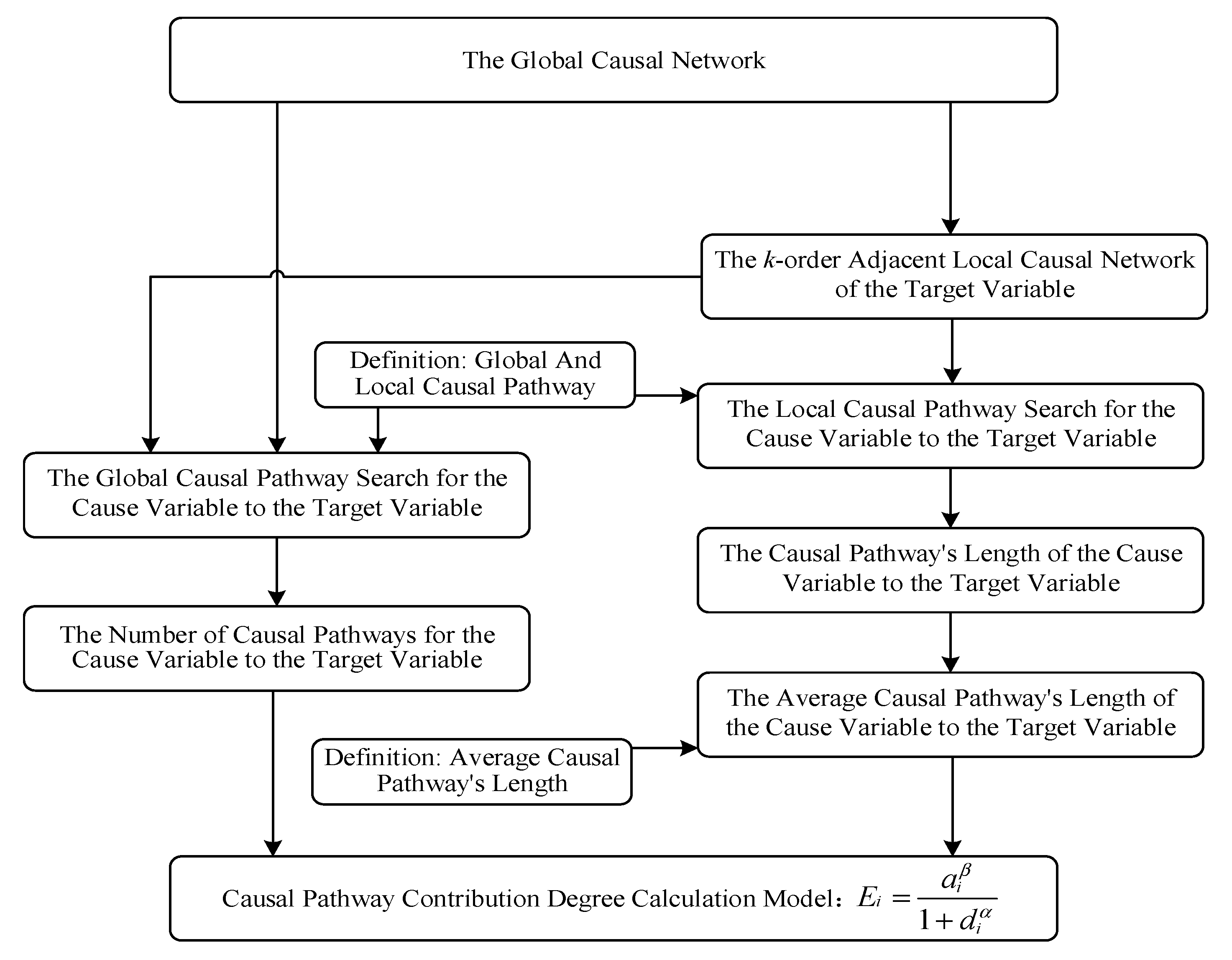
In general, once a global causal network among variables is learned, the causal effects between variables can be calculated using various graph search algorithms combined with quantitative causal inference methods. However, the above calculation process is often very complex and is not feasible for large, dense causal networks. In view of this, a heuristic strategy for approximate causal inference is proposed.
The basic idea of our method comes from perceptual understanding of the physical structure of a causal network. In general, it can be inferred that the more causal pathways through a cause to the target, the greater the causal effect of the cause on the target. Under the same conditions, it can be also inferred that the shorter the causal path length of a cause variable from the target variable, the greater the causal effect of the cause on the target. Based on the basic understanding of the above two aspects, the framework of heuristic causal inference model is shown as
Figure 2.
For the convenience of expression, give the following definitions:
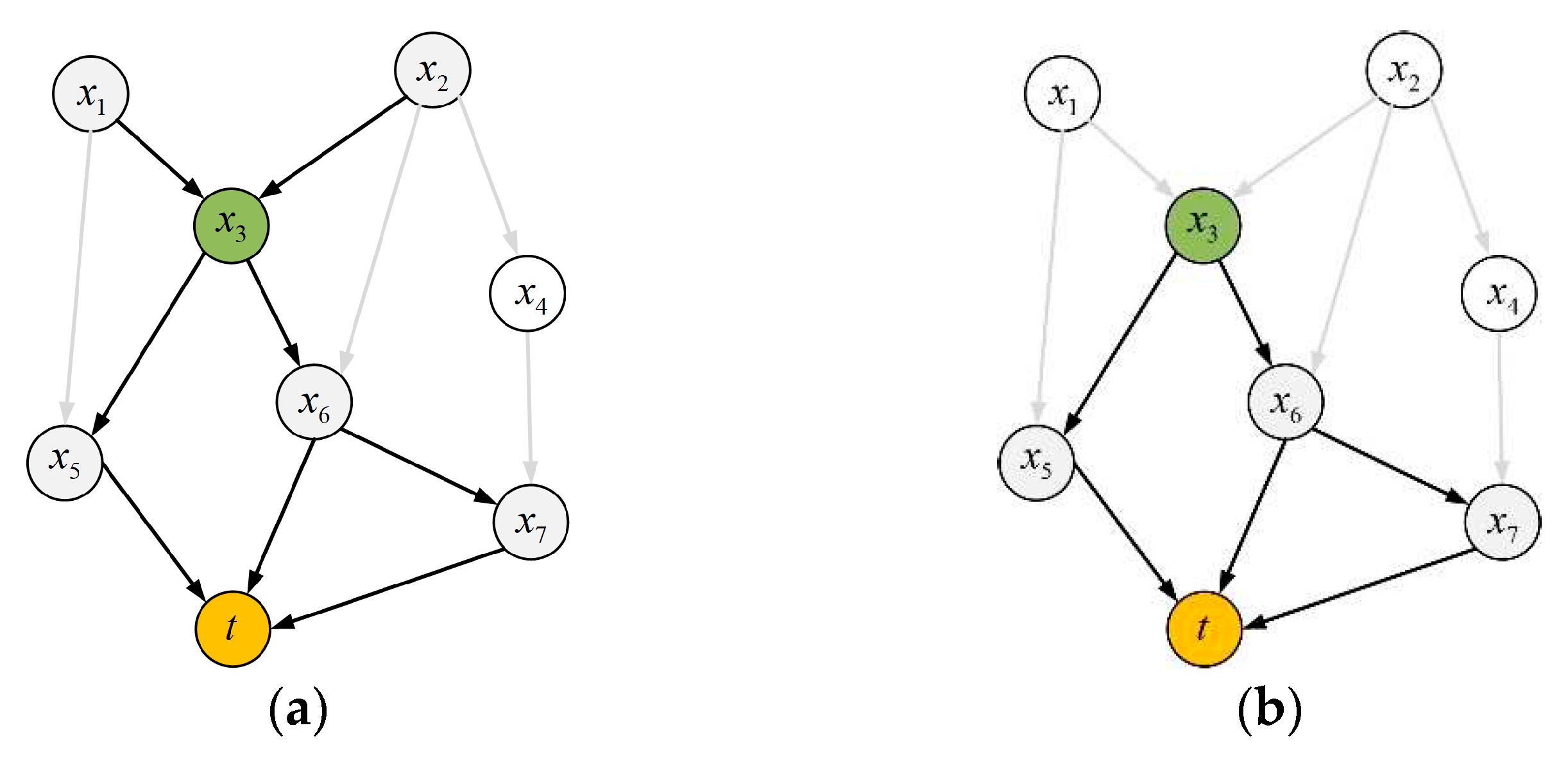
Definition 3: Global Causal Pathway -- In the global causal network, a variable
is the direct or indirect cause of the target variable,
and the causal pathway (
) that points to the target variable
through
is defined as the global causal pathway from
to,
as shown in
Figure 3a.
Definition 4: Local Causal Pathway -- In the global causal network, a variable
is the direct or indirect cause of the target variable,
and the causal pathway (
) that points to the target variable
from
is defined as the local causal pathway from
to,
as shown in
Figure 3b.
According to definitions 3 and 4, if is an end node in a global causal network (has no parent), then the global causal pathway of is the same as its local causal pathway.
In
Figure 3a, there are 9 global causal pathways from
to,
including:
,
,
,
,
,
,
,
and.
In
Figure 3b, there are 3 local causal pathways from
to,
including:
,
and.
Thus, the global causal pathway of
contains its local causal pathway.
Definition 5: Local Causal Pathway’s Length - For a local causal pathway from to, define the total number of direct and indirect causes of on this pathway as its local causal pathway’s length.
In
Figure 3b, the three local causal pathways from
to
have their lengths of 2, 2, and 3, respectively.
Based on definitions 4 and 5, the average causal path length can be defined as follows:
Definition 6: Average Local Causal Pathway’s Length -- Suppose there are
local causal pathways from
to,
and for the
th
of them, its local causal pathway’s length is,
then the average local causal pathway’s length from
to
is:
In
Figure 3, the average local causal pathway’s length from
to
is: (2+2+3)/3=7/3.
Based on definitions 4 to 6, the causal pathway contribution degree of the cause variable to the target variable can be defined as follows:
Definition 7: Causal Pathway Contribution Degree -- In the global causal network,
assume that there are
global causal pathways between the cause variable
and the target variable
; Let the average local causal pathway’s length from
to
be
; Then, the causal pathway contribution degree of
to
is defined as:
Where
is a monotonically increasing function of
and a monotonically decreasing function of,
and
≥0.
Without loss of generality, let:
Where, α and β are adjustment factors greater than zero.
According to the above definitions, the causal effect of the cause variable on the target variable can be approximately calculated: the greater the value of, the greater the causal effect of on,and vice versa.
3.4. Key Influencing Factors Identification
If a certain target variable is selected in a complex system, there are several factors that have a large or small influence on it, and this influence can be measured by causal effect value. Let the set of cause variables of the target variable be, and these cause variables are the influencing factors of.In addition, let the causal effects of on be,then the greater the value of, the greater the causal effect of on. Usually, researchers pay more attention to the first several system factors that have a greater impact on the target variable. Here, these factors are defined as the key influencing factors of the target variable.
In order to identify the key influencing factors of the target,
it is necessary to calculate the causal effect of the cause variable
on.
According to the basic ideas in
Section 3.3, the causal effect can be approximately replaced by the causal pathway contribution degree proposed, that’s to say:
Considering that the longer the causal pathway is, the smaller the causal effect of the end cause variable on the target variable tends to be. Therefore, in the above calculation, the cause variable can be limited to the k-order adjacent local causal network of the target variable.
Sort cause variables
of
in’s
k-order adjacent local causal network according to their causal effects on the target variable,
the rearranged cause variables’ sequence is:
Assuming that for a certain system, only the first
factors that have a decisive influence on the target variable,
the key influencing factors identified based on the proposed method are as follows:
Among them, has the greatest influence on the target variable, has the second influence on the target variable,and so on.
4. Experiments and Results
A semiconductor production system is taken as an example for simulation experiment. Modern semiconductor production often performs quality control by monitoring signals collected from all kinds of sensors. In a specific monitoring environment, the monitoring signal reflects the operation of each node of the production line, and determines the final product quality. If each type of signal is treated as a feature, there is a tight interrelationship between these features. Using the heuristic causal inference method proposed by us, the causal relationship between characteristic variables is funded, and the key factors leading to the fluctuation of product output, which is chosen as the target variable and is labeled as Pass/Fail, are identified finally.
4.1. Experimental Data Introduction and Procession
The experimental dataset SECOM [
34] (Semiconductor Manufacturing) is derived from the UC Irvine machine learning repository [
21]. SECOM consists of production line monitoring data and semiconductor quality data, containing 1,567 observations, each of which is a vector of 590 sensor measurements, plus a Pass/Fail label of the product.
It should be noted that there are some missing values in the dataset, and only 104 of the 1567 observations recorded that the product failed the quality test, while the vast majority of products passed the quality test, with a ratio of about 1:14. To this end, the experimental data was preprocessed, and the main work included: (1) Establish the index of the dataset; (2) Delete columns with more than 50% of their data missing; (3) Interpolate missing values in the data set. In general, each sample’s missing values are imputed using the mean value from n-neighbors nearest neighbors found in the dataset; (4) Normalize the dataset; (5) Eliminate features that have a variation below a specified threshold; (6)Use down sampling technology for data balancing.
After processing, a new experimental data set was formed, including 449 variables, and the sample size was 416 (the ratio of Pass and Fail was 3:1).
4.2. Global Causal Network Learning
The experiment was carried out according to the steps described in
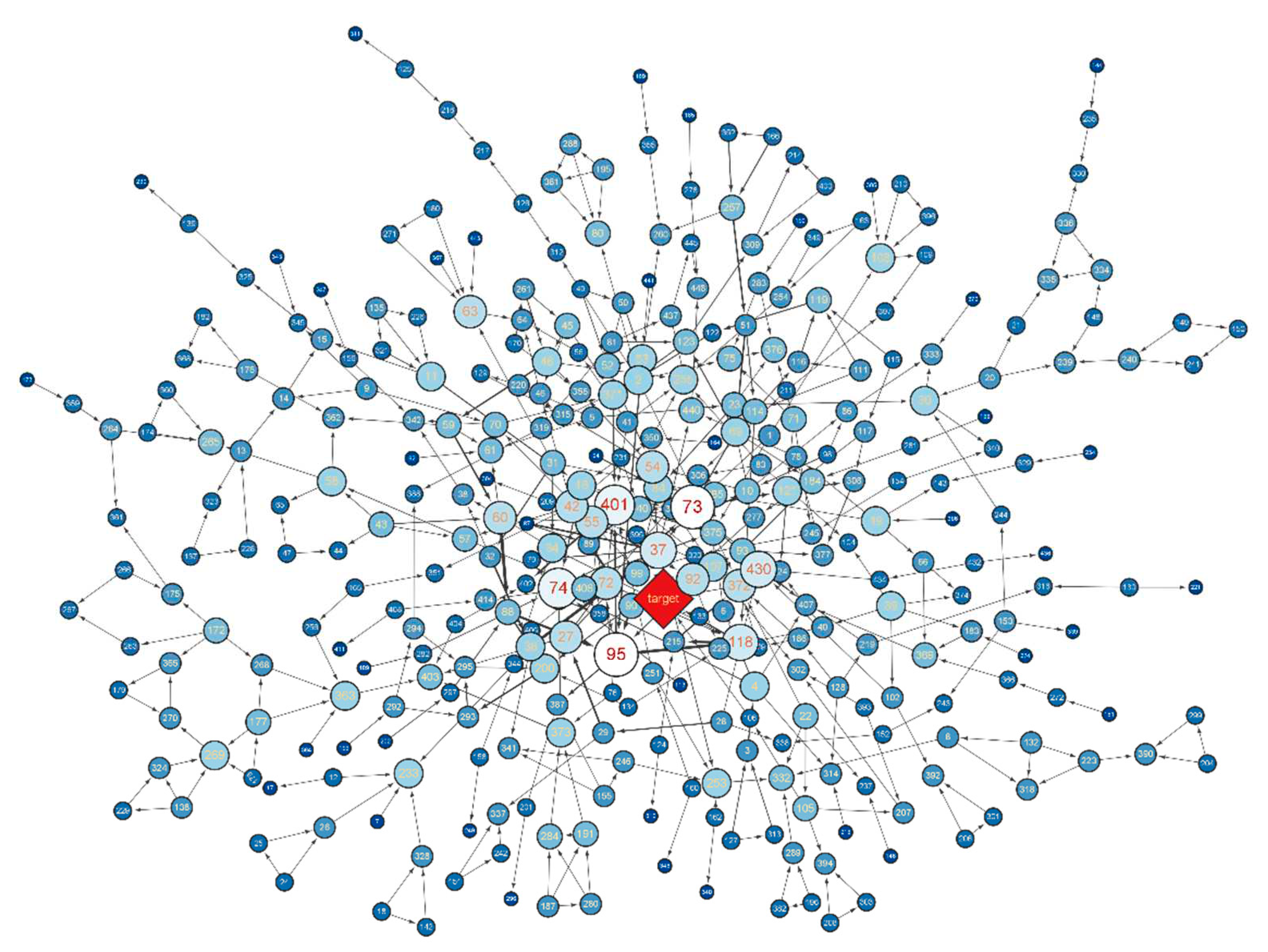
Section 3.2.1. In the process, the significance level of FCI is set to 0.05 and other parameters are set to default. We obtain the global causal network around the target variable as shown in
Figure 4, including 347 nodes and 493 edges. Where, the central node “target” is the selected target variable, which refers to the product test results. The five surrounding nodes (55, 106, 118, 277, 372) form the Markov boundary of the target variable.
The global causal network is analyzed according to the way of complex network, and its network characteristics are shown in
Table 1.
4.3. Local Causal Network Construction
According to the steps in
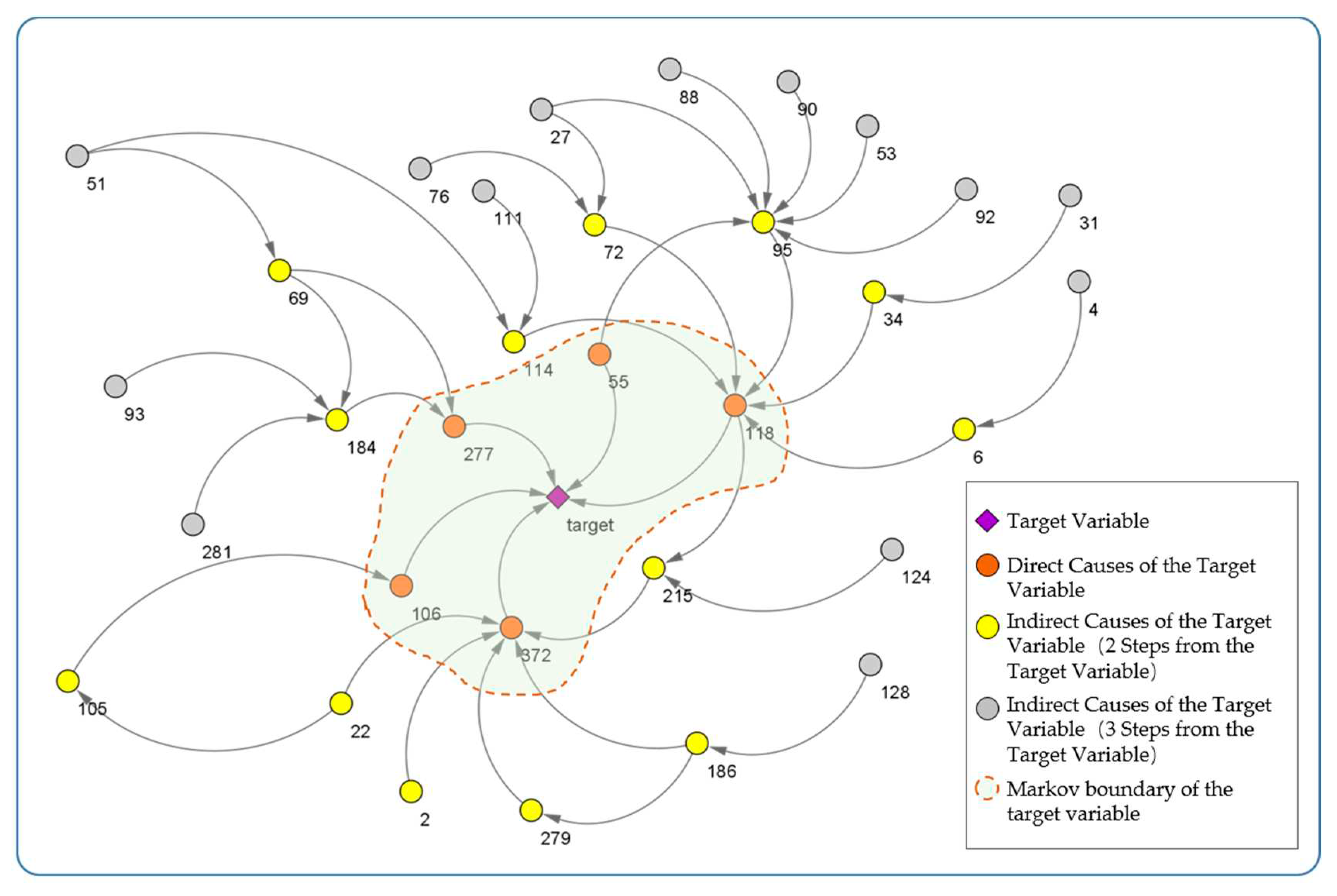
Section 3.2.2, a third-order adjacent local causal network of the target variable is constructed, as shown in
Figure 5.
In this third-order adjacent local causal network, there are 32 direct and indirect cause nodes of the target variable. There are 5 direct cause nodes whose shortest causal pathway length with the target variable is 1 (Markov boundary of the target variable). There are 13 indirect cause nodes whose shortest causal pathway length with the target variable is 2. There are 14 indirect cause nodes whose shortest causal pathway length with the target variable is 3.
4.4. Heuristic Causal Effect Calculation
According to the steps in
Section 3.3, the number of causal pathways, average causal pathway length and causal pathway contribution degree of each direct and indirect cause of the target variable in the local causal network were calculated, and the results are shown in
Table 2.
4.5. Final Results
The causal path contribution degree in
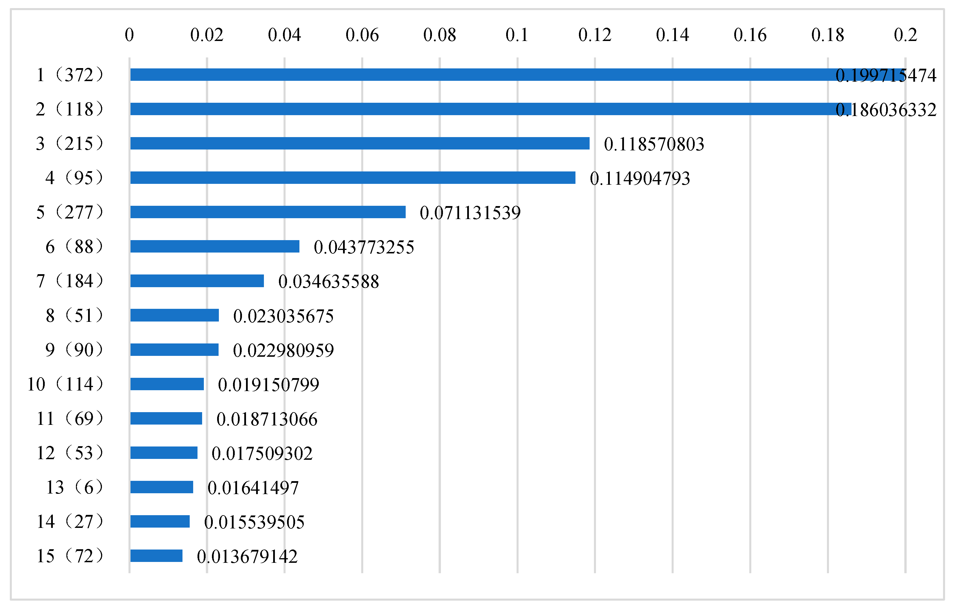
Table 2 is normalized, and the top 15 influencing factors that have a greater impact on the target variable are screened out and sorted according to the ideas in
Section 3.4. The results are shown in
Figure 6. In the figure, node No. 372 is ranked first, and its normalized causal pathway contribution degree is 19.97%. The second node is No. 118, whose normalized causal pathway contribution degree is 18.60%. By analogy, the 15th ranked node is No. 72, whose normalized causal pathway contribution degree is 1.37%.
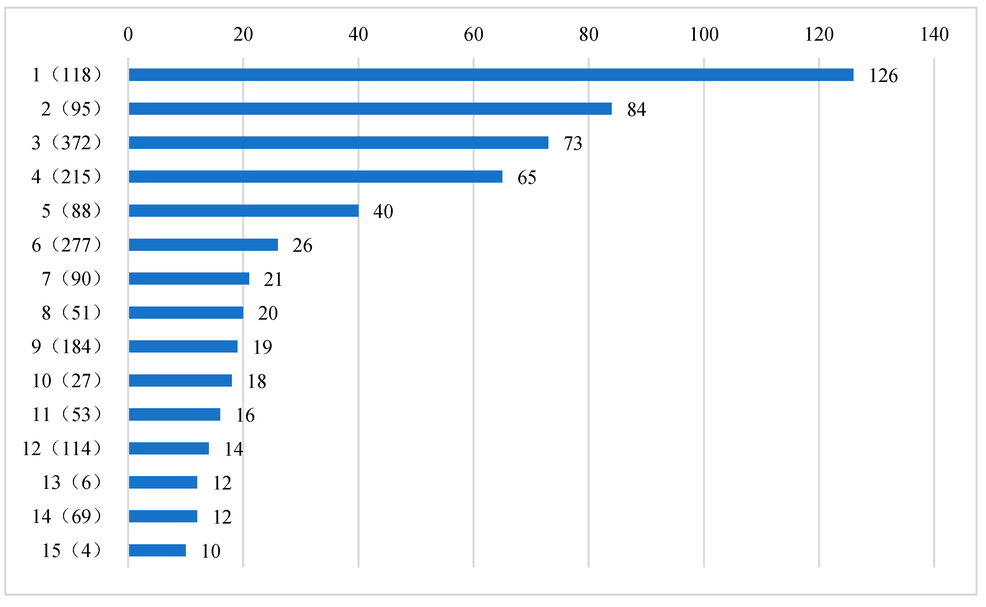
In addition, if only the number of causal pathways pointing to the target variable through a certain cause (direct cause and indirect cause) node is considered, the selected key influencing factors of the target variable are shown in
Figure 7. At this time, the first node is No. 118, and there are 126 global causal pathways through this node to the target variable. The second node is No. 95, and there are 84 global causal pathways to target variables through this node. By analogy, the fifteenth is node 4, and there are 10 global causal pathways through this node to the target variable.
4.6. Further Validation
So far, we have screened out several key influencing factors. In order to verify the correctness of the proposed method, we refer to the evaluation metrics in feature selection and feature extraction [
35,
36] to test the experimental results.
Since our dataset is highly imbalanced, we must not use accuracy as our evaluation metric. Instead, we use F1 Score and Matthews Correlation Coefficient (MCC), which are both suitable measure of models tested with imbalance datasets [
37]. The F1 score is a comprehensive evaluation index, which integrates two evaluation parameters, accuracy rate and recall rate, to evaluate the overall performance of the classifier [
38]. The MCC is in essence a correlation coefficient value between -1 and +1. A coefficient of +1 represents a perfect prediction, 0 an average random prediction and -1 an inverse prediction [
39].
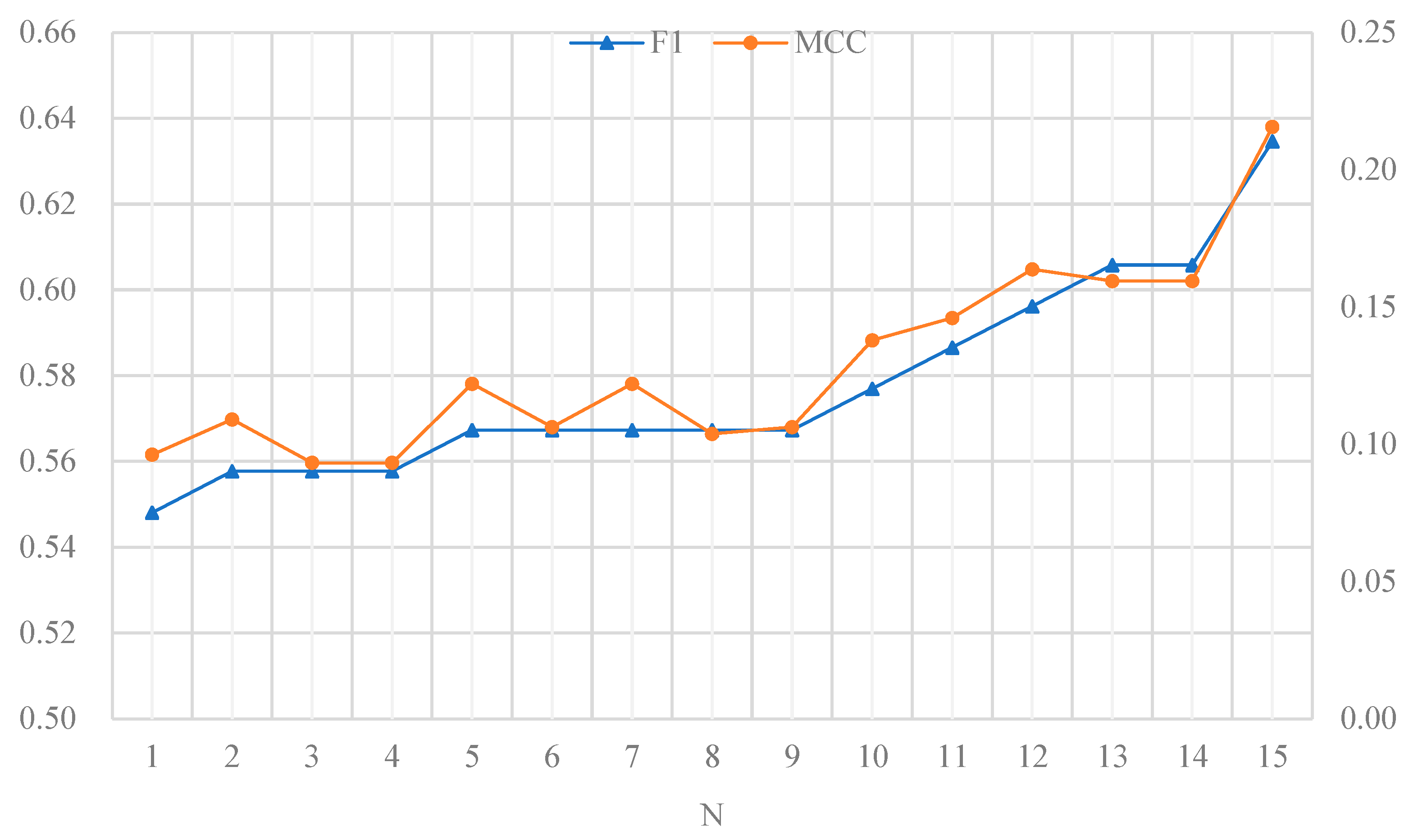
For the preprocessed experimental data set, we set 1/4 of them as the test group and the rest as the training group. A common logistic regression classifier was adopted as the classifier used in the experiment. When we took all 448 feature variables as input of the classifier, we got F1 and MCC values of 0.4216 and 0.0612, respectively. When we took the selected 15 key influencing factors as the input of the classifier, the values of F1 and MCC were 0.6431 and 0.2209 respectively. On this basis, we sorted key influencing factors according to their importance, deleted the first to 15th key influencing factors respectively, and took the remaining key influencing factors as the input of the classifier to obtain the corresponding F1 and MCC evaluation index values respectively. The experimental results are shown in
Figure 8.
In
Figure 8, N=1 indicates that the first key influencing factor is deleted, and the remaining 14 key influencing factors are used as characteristic variables. In this case, the obtained F1 value and MCC value are 0.548 (corresponding to the left ordinate) and 0.096 (corresponding to the right ordinate) respectively. N=2 means that the second key influencing factor is deleted, and the other remaining 14 key influencing factors are used as characteristic variables, and so on.
5. Discussion
It can be seen from
Figure 6 that, among the 15 key influencing factors, three of them are the direct causes of the target variable, and 10 of them are included in the second-order local causal network of the target variable. Among them, the three direct causes of the target variable have a great impact on the causal pathway pointing to the target variable in the global causal network, and the normalized causal pathway contribution degree is 19.97%, 18.60% and 7.11%, respectively, which also indicates that the direct cause node on the Markov blanket has a decisive impact on its corresponding target variable.
In combination with
Figure 5 and
Figure 6, it can also be concluded that some indirect causes also have higher causal pathway contribution degrees to the target variable, and a few indirect causes have greater causal pathway contribution degree to the target variable than other direct causes. For example, the two indirect causes numbered 215 and 95 have a higher causal pathway contribution degree to the target variable than the three direct causes numbered 55, 106 and 277. Among them, the normalized causal pathway contribution degree of node 215 is 11.86%, and the normalized causal pathway contribution degree of node 95 is 11.49%.
By comparing
Figure 6 and
Figure 7, it can be seen that when only the number of causal pathways is considered, the key influencing factors of the target variable are basically consistent with those when the number of causal pathways and the length of causal pathways are considered simultaneously. In both results, only one factor changed: Node No. 72, which ranked 15th in
Figure 6, was changed to node No. 4, which ranked 15th in
Figure 7. However, the ranking of key influencing factors in the two results has changed significantly: only the ranking of node 51 in the 8th ranking and node 6 in the 13th ranking remain unchanged. Considering that the influence of the cause variable on the target variable will gradually decrease with the length growth of the causal pathway, it is more scientific to calculate the contribution degree of the causal pathway by comprehensively considering the number of causal pathways and the length of causal pathways.
It can be seen from the experimental results in
Section 4.6 that when all characteristic variables are taken as inputs to the classifier, the classifier’s prediction performance is relatively poor, and F1=0.4216, MCC=0.0612。When we use the selected 15 key influencing factors as characteristic variables, the prediction performance of the classifier was greatly improved, and F1=0.6431, MCC=0.2209. This also confirms the theoretical basis of feature selection: for a given sample size, there is a maximum number of features above which the performance of our classifier will degrade rather than improve in most cases, the additional information that is lost by discarding some features is (more than) compensated by a more accurate mapping in the lower-dimensional space. As can be seen from
Figure 8, when we successively delete the key influencing factors ranked 1-15 and take the remaining 14 key influencing factors as the feature variables, the prediction performance of the classifier is gradually improved—the values of F1 and MCC both gradually increase. This also shows from another aspect that there are indeed differences in the specific impacts of the selected key influencing factors on the system. The higher the ranking of key influencing factors, the greater the corresponding impact on the system.
In general, simulation experiments based on SECOM dataset obtained causal networks among variables that drive the dataset generation. Based on the heuristic causal inference method proposed in this paper, several factors that have a key impact on product quality were identified. The achievement has certain guiding significance for understanding the monitoring data in semiconductor production. In an ideal situation, the overall operation of the production line can be determined by analyzing the monitoring data corresponding to the direct cause of the target variable. When the monitoring data of some direct causes cannot be obtained, the analysis of the monitoring data corresponding to the key indirect causes can also be meaningful. For the craftsmen on the production line, the targeted operation and maintenance guarantee according to the key influencing factors can reduce the unit production cost and improve the overall efficiency of the system.
6. Conclusions
In view of the natural advantages of causal inference in revealing the essential law of things, a heuristic causal inference method for identifying the key influencing factors of complex systems is proposed. On the basis of acquiring the causal network among variables by using observational data, the direct cause and indirect cause of the target variable are defined, and the global causal pathway, local causal pathway and average causal pathway length from cause variable to the target variable are defined. By referring to the analysis method of complex network, the causal pathway contribution degree is proposed to replace the causal effect of the cause variable on the target variable. Based on this, the heuristic causal inference is carried out, which can quickly realize the identification of the key influencing factors of the system from the perspective of causality.
Simulation experiments are carried out on SECOM dataset, and a causal network consisting of 347 nodes and 493 edges is obtained. Taking product quality test results as the target variable, the key influencing factors are identified. Based on the modeling analysis process and the experimental results of our research, the following conclusions can be drawn:
(1) It is feasible to analyze complex systems through causal science, and the causal network that drives the generation of system monitoring dataset can be obtained by combining the traditional causal discovery method with domain prior knowledge;
(2) The heuristic causal inference method proposed in this paper can solve the problem that it is difficult to identify key influencing factors in complex systems. The core index of heuristic causal inference - causal path contribution degree can scientifically reflect the causal impact of cause variables on the target variable, and can be quantitatively calculated with low computational complexity.
In the next step, we can further explore the deep integration of the theories and methods related to complex networks and causal inference, and combine the advantages of both to promote a deeper understanding of some other complex systems.
Author Contributions
J.W.: conceptualization, writing—original draft, writing—reviewing and editing, methodology, validation, formal analysis. Y.L.: supervision, writing—reviewing and editing. D.L.: supervision, data procession, formal analysis. W.Z.: supervision, writing—editing. J.H.: supervision, writing—editing. All authors have read and agreed to the published version of the manuscript.
Funding
This research received no external funding.
Institutional Review Board Statement
Not applicable.
Informed Consent Statement
Not applicable.
Data Availability Statement
The dataset and code generated during the current study are not publicly available, because the data and code also form part of the ongoing study, but they can be obtained from the corresponding authors according to reasonable requirements.
Acknowledgments
The authors thank all reviewers who helped to improve this manuscript.
Conflicts of Interest
The authors declare no conflict of interest.
References
- Di, Z.; Chen, X. Complex systems science: recent advances. J.BNU (NSCI), 2022, 58, 371–381. [Google Scholar]
- Orlando, G.; Mariya, G. Complex systems in economics and where to find them. J. Syst. Sci. & Complex. 2021, 34, 314–338. [Google Scholar]
- Alvarez, J. T.; Patricio, R-C. A brief review of systems, cybernetics, and complexity. Complex. 2023, 2023, 1. [Google Scholar] [CrossRef]
- Yu, S; Hu, G.; Zhang, Y.; et al. Eigen microstates and their evolutions in complex systems. Commun. Theor. Phys. 2021, 73, 1. [Google Scholar]
- Ding, Z.; Liu, X.; Xue, Z.; et al. Expert opinion on the key influencing factors of cost control for water engineering contractors. Sustain. 2023, 15, 6963. [Google Scholar] [CrossRef]
- Lin, X.; Xia, S.; Luo, Y.; et al. Evaluation of key factors influencing urban ozone pollution in the Pearl River Delta and its atmospheric implications. Atmos. Environ. 2023, 305, 119807. [Google Scholar] [CrossRef]
- Ghiwa, A.; Rayan, H. A. Key decision-making factors influencing bundling strategies: analysis of bundled infrastructure projects. J. Infrastruct. Syst. 2023, 29, 1–16. [Google Scholar]
- Listl, S. M.; Matsuyama, Y.; Jürges, H. Causal inference: onward and upward. J. Dental Res. 2022, 101, 877–879. [Google Scholar] [CrossRef] [PubMed]
- Mitra, N.; Roy, J.; Small, D. Future of causal inference. Am. J. Epidemiology, 2022, 191, 1671–1676. [Google Scholar] [CrossRef]
- Cai, R.; Chen, W.; Zhang, K. et al. A Survey on non-temporal series observational data based causal discovery. Chin. J. Comp. 2017, 40, 1470–1490. [Google Scholar]
- Liu, J.; Zhang, X.; Li, X.; Li, Z.; Sun, C. A new quantitative evaluation index system for disaster-causing factors of mud inrush disasters in water-rich fault fracture zone. Appl. Sci. 2023, 13, 6199. [Google Scholar] [CrossRef]
- Nguyen, T. S.; Chen, J-M.; Tseng, S-H.; et al. Key factors for a successful OBM transformation with DEMATEL–ANP. Maths. 2023, 11, 2439. [Google Scholar] [CrossRef]
- Abdullah, F. M.; Al-Ahmari, A. M.; Anwar, S. An integrated fuzzy DEMATEL and fuzzy TOPSIS method for analyzing smart manufacturing technologies. Proc. 2023, 11, 906. [Google Scholar] [CrossRef]
- Wang, Y.; Guo, W.; Bai, E.; Wang, Y. Key strata identification of overburden based on magneto telluric detection: a case study. Appl. Sci. 2020, 10, 558. [Google Scholar] [CrossRef]
- Rong, Y.; Xiong, T.; Huang, H.; et al. Identification and analysis of key factors of propellant cross-feed system in launch vehicle. J. Astronautics, 2021, 42, 239–248. [Google Scholar]
- Zhang, Q.; Zhang, Y.; Cheng, Z.; et al. Static behavior and key influencing factors of double-cable suspension bridge. J. SWJTU, 2020, 55, 238–246. [Google Scholar]
- Chen, J.; Zhai, G.; Wang, S.; et al. Factors affecting characteristics of acoustic signals in particle impact noise detection for aerospace devices. Syst. Eng. Electron. 2013, 35, 889–894. [Google Scholar]
- Sun, Y.; Zhou, T.; Chen, G.; et al. Quantitative analysis of key factors affecting struvite crystal growth rate. CIESC J. 2021, 72, 5831–5839. [Google Scholar]
- Sun, Y.; Han, W.; Duan, W. Review on research progress of DEMATEL algorithm for complex systems. Contr. & Dec. 2017, 32, 385–392. [Google Scholar]
- Si, S.; You, X.; Liu, H.; et al. DEMATEL technique: a systematic review of the state-of-the-art literature on methodologies and applications. Math. Prob. Eng. 2018, 1, 1–33. [Google Scholar] [CrossRef]
- Sun, Y.; Huang, Z; Li, Y. Review of state of the art on DEMATEL algorithms for complex factor analysis. J. Front. Comp. Sci. & Tech. 2022, 16, 541–551. [Google Scholar]
- Zhang, Y.; Rong, X.; Shu, M.; et al. Identification of key influencing factors of user experience of mobile reading APP in China based on the fuzzy-DEMATEL model. Math. Prob. Eng. 2021, 1, 1–12. [Google Scholar] [CrossRef]
- Li, S.; Ma, Y.; Zhu, E. Analysis of institutional barriers to integrated innovation based on AHP-DEMATEL. J. HEU. 2022, 43, 900–906. [Google Scholar]
- Chiu, Y.; Hu, Y.; Yao, C.; et al. Identifying key risk factors in product development projects. Math. 2022, 10, 1295. [Google Scholar] [CrossRef]
- Altuntas, F.; Gok, M. S. The effect of COVID-19 pandemic on domestic tourism: A DEMATEL method analysis on quarantine decisions. Int. J. Hosp. Manage. 2021, 92, 102719. [Google Scholar] [CrossRef] [PubMed]
- Li, Y.; Zhao, K.; Zhang, F. Identification of key influencing factors to Chinese coal power enterprises transition in the context of carbon neutrality: A modified fuzzy DEMATEL approach. Energy, 2023, 263, 125427. [Google Scholar] [CrossRef]
- Mazzuto, G.; Stylios, C.; Ciarapica, F. E.; et al. Improved decision-making through a DEMATEL and fuzzy cognitive maps-based framework. Math. Prob. Eng. 2022, 1–14. [Google Scholar] [CrossRef]
- Sait, G. Spherical fuzzy extension of DEMATEL(SF-DEMATEL). Int. J. Intell. Syst. 2020, 35(9), 1329–1353. [Google Scholar]
- Colombo, D.; Maathuis, M. H.; Kalisch, M.; et al. Learning high-dimensional directed acyclic graphs with latent and selection variables. Comp. Sci. 2011, 40, 294–321. [Google Scholar] [CrossRef]
- Spirtes, P.; Glymour, C.; Scheines, R. Causation, Prediction, and Search, 2nd ed.; MIT Press, Cambridge, Eng. 2000; 144-145.
- Marx, A.; Vreeken, J. Causal discovery by telling apart parents and children. Stat. 2018, 2, 1–11. [Google Scholar]
- Colombo, D.; Maathuis, M. H.; Kalisch, M.; et al. Supplement to “Learning high-dimensional directed acyclic graphs with latent and selection variables.”.
- Zhang, J. On the completeness of orientation rules for causal discovery in the presence of latent confounders and selection bias. Artif. Intell. 2008, 172, 1873–1896. [Google Scholar] [CrossRef]
- Paresh, M. UCI SECOM Dataset [EB/OL]. https://www.kaggle.com/datasets/paresh2047/uci-semcom.
- Ladla, L.; Deepa, T. Feature selection methods and algorithms. IJCSE 2011, 3(5), 1787–1797.
- Samina, K.; Tehmina, K.; Shamila, N. A survey of feature selection and feature extraction techniques in machine learning. In Proceedings of the 2014 Science and Information Conference, London, UK, 27-29 August 2014; pp. 372–378. [Google Scholar]
- Chicco, D.; Jurman, G. The advantages of the Matthews correlation coefficient (MCC) over F1 score and accuracy in binary classification evaluation. BMC genomics 2020, 21(1), 6. [Google Scholar] [CrossRef] [PubMed]
- Chinchor, N. MUC-4 evaluation metrics. In Proceedings of the 4th conference on Message understanding (MUC4 ’92). Association for Computational Linguistics, USA; 1992; pp. 22–29. [Google Scholar]
- Baldi, P.; Brunak, S.; Chauvin, Y.; et al. Assessing the accuracy of prediction algorithms for classification: an overview. Bioinformatics 2000, 16(5), 412–24. [Google Scholar] [CrossRef] [PubMed]
|
Disclaimer/Publisher’s Note: The statements, opinions and data contained in all publications are solely those of the individual author(s) and contributor(s) and not of MDPI and/or the editor(s). MDPI and/or the editor(s) disclaim responsibility for any injury to people or property resulting from any ideas, methods, instructions or products referred to in the content. |
© 2023 by the authors. Licensee MDPI, Basel, Switzerland. This article is an open access article distributed under the terms and conditions of the Creative Commons Attribution (CC BY) license (http://creativecommons.org/licenses/by/4.0/).
