Submitted:
16 August 2023
Posted:
17 August 2023
You are already at the latest version
Abstract
Breast cancer is the most common malignancy in women worldwide. The pathogenesis of this disease is closely related to the estrogen receptor alpha subtype (ERα). Therefore, it is of great importance to develop effective inhibitors of ERα activity for the treatment of breast cancer. In this paper, we propose a novel ensemble machine learning model for quantitative structure-activity relationship of anti-breast cancer drugs, which can effectively predict drug activity in small samples with multiple characteristic variables. To avoid the problem of over-fitting caused by low-correlation independent variables, the scoring mechanism of random forest was improved by incorporating three relevance indicators, including the maximum mutual information number, Pearson correlation coefficient and distance correlation coefficient, and 20 optimal molecular descriptors were selected. The Bayesian hyperparameter optimization method was used to optimize the parameters of multiple linear regression (MLR), support vector regression (SVR), and extreme gradient boosting (XGBoost), respectively. The AdaBoost strong learner was constructed by combining the weak learner with the weighted linear addition method. The results show that the proposed ensemble learning model has the best prediction performance compared to the three basic learner models and the CNN-LSTM combination prediction model. The root mean square error was reduced by 7.60%-26.51%. The mean relative error was reduced by 6.46%-30.92%. Goodness of fit increased by 9.57%-36.94%. Finally, the biological activities of 50 candidate compounds for ERα inhibitors were predicted, and it was found that 4-[2-benzyl-1-[4-(2-pyrrolidin-1-ylethoxy)phenyl]but-1-enyl]phenol had an excellent biological activity value pIC50, which had the potential to be an ERα inhibitor. The model proposed in this paper has good prediction accuracy, which can provide an effective reference for the discovery and development of anti-breast cancer drugs.
Keywords:
Breast cancer
; Activity prediction
; Random forest
; Feature selection
; Bayesian hyperparameter optimization
; AdaBoosting
1. Introduction
Breast cancer is one of the most common cancers with a high mortality rate in the world and is the leading cancer among women worldwide, as shown in Figure 1. According to data published by the International Agency for Research on Cancer (IARC) of the World Health Organization, the number of new cases of breast cancer worldwide will reach 2.26 million in 2020, and breast cancer will replace lung cancer as the fastest growing cancer in the world [1]. The distribution of the highest cancer incidence in women worldwide is shown in Figure 1. According to statistics, approximately one in three people in the United States will be diagnosed with cancer, and one in eight women will develop breast cancer. The global incidence of breast cancer is expected to increase to 3 million cases by 2040 [2]. Although the mortality rate from breast cancer has decreased over the past two years due to improvements in medical care, the incidence and disease burden of breast cancer are still slowly increasing each year [3], threatening the health of women worldwide.
There are significant regional differences in the incidence of breast cancer in women, as shown in Figure 2.
The figure above shows that the incidence of breast cancer is relatively low in Asian and African countries and relatively high in the Americas and Oceania. In addition, the higher the level of economic development in Europe and the United States, the higher the incidence of breast cancer among women. However, scholars have found that the reporting age of women in some Asian countries is generally earlier than that in Europe [5], and the incidence of breast cancer has shown a rapidly increasing trend in recent years due to economic transformation and lifestyle changes [6].
The development of breast cancer is closely associated with estrogen receptors. Related studies have shown that estrogen receptor alpha (ERα) is expressed in less than 10% of normal breast epithelial cells, but in approximately 60% of breast tumor cells [7,8]. Experimental results in mice by Tekmal et al. [9] showed that mammary gland development in mice lacking the ERα gene would be impaired even in the presence of persistent tissue estrogen, demonstrating that ERα plays an important role in mammary gland development and induces mammary gland hyperplasia in mice. In addition, Lee et al. [10] further demonstrated through whole genome sequencing (WGS) that the disruption and translocation of the ERα genome in estrogen is a direct factor influencing breast cancer gene expansion. Therefore, estrogen is considered to be one of the important pathogenesis of breast cancer, and ERα is considered to be an important target.
In the treatment process, estrogen receptor activity plays an important role in controlling estrogen levels in the body, especially in anti-hormone therapy, which is commonly used in ERα-expressing breast cancer patients [11]. This means that compounds that can inhibit the activity of ERα may be the key drugs for the treatment of breast cancer, such as transcription factor activating protein 2γ (TFAP2C, AP-2γ) [12] and aromatase inhibitors [13]. Good anti-breast cancer activity is an important evaluation index for the selection of inhibitors. Therefore, in recent years, more and more scholars have adopted the method of establishing compound activity prediction models to screen anti-breast cancer candidate drugs [14,15,16]. The accurate prediction model and the key factors affecting the biological activity of estrogen receptor α subtype, the therapeutic target of breast cancer, have become the focus of medical attention.
The main contributions of this paper are as follows: (1) The advantages of the maximum information coefficient method, distance correlation and Pearson correlation are integrated, and the traditional random forest method is improved to compensate for the disadvantages of the lack of variable correlation in the feature selection process of the traditional random forest, so as to better filter out the optimal molecular descriptors. (2) The Bayesian hyperparameter optimization method is adopted to optimize the hyperparameters of the XGBoost model, so as to effectively improve the prediction accuracy and generalization ability of the model. (3) In this paper, the above research methods are applied to drug activity prediction studies for the first time, and the biological activities of 50 new anti-breast cancer candidates are verified. At the same time, this method can also be used to solve other drug activity prediction problems. These contributions make this study have important scientific significance and practical application prospect.
The rest of this paper is organized as follows: Section 2 summarizes the literature on drug activity prediction from both traditional experimental methods and machine learning methods. Section 3 introduces the data used in this study and preprocesses the dataset. In Section 4, we present our improved random forest feature selection method and a comprehensive prediction model for the activity of ERα inhibitors against breast cancer. In Section 5, the dataset is divided into test and training sets, and the model proposed in this paper is used for empirical analysis. In Section 6, the rationality and accuracy of this model were verified by comparing with other classical drug activity prediction models, and the biological activities of 50 new candidate compounds were predicted. In Section 7, the main results of this paper are summarized and the direction for future improvement is suggested.
2. Related Work
With the rapid development of drug research and development, many drug activity prediction methods have emerged. After reviewing important literature, drug activity prediction methods can be divided into two categories: traditional experimental methods and machine learning methods.
2.1. Traditional Experimental Method
This type of method is characterized by the fact that no machine learning algorithms are used in the computational process. The application of drugs in the treatment of diseases is regarded as a complex interaction process between drug molecules and corresponding target proteins [17]. At present, the study of drug-target protein interaction is mainly divided into experimental methods and computational methods.
2.1.1. Experimental Method
Nuclear magnetic resonance (NMR) spectroscopy can accurately probe the distribution of metabolites in living cells and tissues in vivo and identify lead compounds that inhibit protein interactions [18]. Mansa et al. [19] found that isothermal microcalorimetry (IMC) has more potential than agar diffusion and broth culture in determining the antimicrobial activity of probiotic isolates. Surface plasmon resonance (SPR) has been used by scientists for secondary screening, lead optimization, and quantitative structure-activity relationship analysis [20]. KenIchiro et al. [21] used structure-based high throughput screening (HTS) to discover the multifunctional chemical inhibitors of florigen activation complex.
However, these experimental methods have the limitations of high cost, long time and small application range, so the computer-aided drug target prediction method is more favored by researchers in the traditional experimental methods.
2.1.2. Computer Aided Method
Computational methods have undergone continuous development and enrichment from the earliest ligand-based prediction methods, to structure-based prediction methods, to molecular dynamics prediction methods.
The ligand-based prediction method is to analyze the three-dimensional structure of drug molecules for activity prediction, and the quantitative structure-activity relationship (QSAR) proposed by Hansch et al. [22] has been widely used in drug activity prediction. For example, Mansouri et al. [23] trained estrogen or androgen receptor activity prediction by various QSAR methods, and Putri et al. [24] used QSAR to establish a prediction model for anti-colon cancer and anti-liver cancer activity of substituted 4-anilylmarin derivatives.
Structure-based methods, which are widely used in molecular docking and virtual screening (VS), predict the activity of target proteins by analyzing the three-dimensional structure of the target protein. Both molecular docking and virtual screening predict the activity and selectivity of drugs by simulating and evaluating the interaction between drug molecules and target molecules. Wang et al. [25] first proposed the protein-ligand scoring method (SCORE), which introduced the atomic binding score and used the empirical scoring function to represent the binding free energy, and then calculated the binding affinity between the protein with known three-dimensional structure and the corresponding ligand. In addition, empirical scoring methods include DrugScore [26] based on knowledge, genetic optimization for ligand docking (GOLD) [27] based on force field, and VALIDATE [28] based on statistical methods, and so on. These functions effectively discriminate between well-docked protein-ligand binding modes.
Molecular dynamics simulation is a research method using computer simulation, which can realize the search of receptor concept, the selection of the best binding site of small molecules, and the evaluation of the binding strength between drug molecules and target proteins in the study of drug activity. The molecular dynamics simulation of Yang et al. [29] showed that the candidate compound had stable binding ability between the two proteases at the same time, thus finding a new potent dual-target inhibitor that can be used for cancer treatment. Xiao et al. [30] investigated the conformational changes of GLP-1R in the activation process by accelerated molecular dynamics and conventional molecular dynamics simulation, and obtained the intermediate states and their effects of different helices in the activation process by structural analysis and potential of mean force (PMF) calculation.
2.2. Machine Learning Method
With the rapid development of biomedicine, drug activity data is showing a rapid growth trend. The use of traditional experimental methods to predict drug activity can no longer meet the needs of new drug research and development. Machine learning has a good ability to express the deep level of high-dimensional data, and scholars have found that the accuracy of drug activity prediction can be greatly improved by using algorithms [31]. Related research can be divided into traditional machine learning methods and some new directions of machine learning in recent years, such as deep learning and ensemble learning.
2.2.1. Traditional Machine Learning Methods
Traditional machine learning methods mainly include support vector machine, decision tree, Bayes, stepwise regression, and so on.
Martinčič et al. [32] used machine learning methods of support vector regression and multiple linear regression to predict antioxidant activity, and proposed a new method for graphical evaluation of the applicable range of the support vector regression (SVR) model. Dutt et al. [33] combined decision tree algorithm and moving average analysis method in their study to predict agonist activity of G protein-coupled receptor-40. Lane et al. [34] used the Bayesian model to learn from a library of more than 1000 synthesized molecules. Under the threshold of 100 nM and 1 μM, the average accuracy of predicting the in vitro activity of Mycobacterium tuberculosis was as high as 0.93 and 0.89, respectively, showing excellent performance for a single machine learning algorithm. Hrynkiewicz et al. [35] used forward and backward stepwise regression methods (FR and BR) to predict the structural biological activity of angiotensin converting enzyme (ACE) inhibitor/bitter dipeptide, respectively, and found that C-atC(-) and N-Molw(+) had dual functions on dipeptides. And there was no direct relationship between ACE inhibition and the bitterness of dipeptides.
2.2.2. Deep Learning Method
Deep learning models have been developed to predict inhibitors of various targets, including kinases, and have been shown to achieve better prediction performance than traditional machine learning. Among them, the deep learning neural network (DNN) model is the most widely used and has the highest maturity [36,37,38], including single-task DNN, multi-task DNN, bypass DNN, etc. Convolutional neural network (CNN) is widely used in molecular image learning to identify molecular features in the field of drug activity prediction. For example, Hentabli et al. [39] developed a molecular matrix format adapted from two-dimensional fingerprint descriptors to predict the biological activity of compounds based on deep learning convolutional neural network. The area under the curve (AUC) of the CNN activity prediction method was the highest. Dadfar et al. [40] used genetic algorithm (GA) to optimize the parameters of artificial neural network (ANN) and established the activity prediction model of sulfonamides, and the results showed that the prediction effect was better than genetic algorithm-multiple linear regression (GA-MLR).
2.2.3. Integrated Learning Method
In recent years, ensemble learning models have been gradually applied to drug activity prediction, but there are still relatively few studies. Boosting is one of the most important strategies in ensemble learning. Afolabi et al. [44] used a combination of different boosting methods (Adaboost) to predict new bioactive molecules in order to find pharmacologically active molecules that can provide remedies for a range of different diseases and infections. They conducted research experiments using the widely used molecular diagnostic laboratories (MDL) drug data reporting (MDDR) database and found that the Adaboost method produced better results than other machine learning methods; Tavakoli et al. [45] developed a boosting-enhanced ensemble algorithm (AdaBoost R3) for predicting the biological activity of tyrosine kinase inhibitors, which improved the prediction accuracy of the traditional boosting model and made it free from the influence of outliers. Rong et al. [14] proposed a regression prediction model for the biological activity of ERα of improved sparrow search algorithm-random forest (ISSA-RF), and optimized the parameter range of random forest by an improved sparrow search algorithm to improve the prediction accuracy and efficiency of anti-breast cancer drug candidates. In addition, ensemble learning models such as rotation forest [46] and gradient boosting decision tree (GBDT) [47] have also been applied in drug activity prediction research.
In summary, the research methods of drug activity prediction have gradually diversified from pure biochemical experiments to the support of machine learning algorithms, and then to the application of deep learning and ensemble learning algorithms. Compared with traditional experimental methods, traditional machine learning algorithms save research and development costs and have higher efficiency. However, with the increase of data volume, the performance of traditional machine learning models starts to decline. At present, more and more researchers tend to introduce transfer learning and attention mechanism into deep learning models to shorten the model training time, which greatly improves the prediction accuracy of drug molecules and the effectiveness of drug molecule generation. However, it should be noted that deep learning models sometimes have problems such as overfitting or gradient disappearance, which makes the model unable to effectively learn and further apply the data samples, that is, the generalization performance is not good enough. Data preprocessing and model structure optimization should be the main tasks of further research. Due to the limited prediction accuracy and generalization ability of individual classifiers, some scholars have turned to ensemble learning methods using ensemble classifiers. However, the application of ensemble learning in biomedicine is not mature enough, and the prediction model is relatively single. Second, most of the existing studies mainly focus on using different models for prediction, and select the best prediction method by comparing the performance without further optimizing the model itself. For example, some important hyperparameters in the model often choose empirical values. In addition, there are few studies on the combination of ensemble learning and machine learning algorithms for drug activity prediction.
3. Data Preprocessing
The data used in this paper are from the Drug molecular database of the University of Alberta Drug Bank [48]. The dataset contains the biological activity value pIC50 of 1974 candidate compounds against ERα, as well as the molecular descriptor information of the compounds. Higher pIC50 values indicate higher biological activity. Molecular descriptors include 2D/3D features such as physicochemical properties of the compound (e.g. molecular weight, LogP, etc.), topology (e.g. number of hydrogen bond donors, number of hydrogen bond receptors, etc.).
After statistical screening, there were no empty values in this data set. The number of compounds, i.e. the number of samples, is 1974 and the number of variables, i.e. the number of molecular descriptors, is 729. There is no gap between the number of samples and the number of features. Without any treatment, when the model-based regression algorithm is used for feature selection, it is easy to cause serious overfitting. Therefore, this paper first preprocessed the data set at a deep level, used low-variance filtering to remove invalid variables with low-variance features, and then used Laida criterion to eliminate abnormal variables to obtain high-quality sample data.
3.1 Descriptive Statistics
Descriptive statistical analysis was performed on the biological activity data of 1974 compounds and the data of 729 molecular descriptors, and the results are shown in Table 1.
As can be seen from Table 1, the statistical values of molecular descriptors as a whole are very different, the law of data structure is not obvious, and it is difficult to directly analyze and predict. In addition, the sample data corresponding to 225 molecular descriptors are all 0, and there is data redundancy. These independent variables will be eliminated in the next data preprocessing.
3.2 Elimination of Low Variance Characteristics
All values of the column characteristics of the low-variance function variables are basically the same, the data range does not vary much, the variance is very small, and this type of variable can provide little or no information (such as constant variables and zero-variance variables). In this case, this type of function should be deleted. Low variance filtering is a common feature selection method, which can quickly identify the features with low variance and delete them from the data set to avoid the noise or misleading the model caused by low variance features [49]. In this paper, low variance filtering is used to preprocess the data.
Since the variance is related to the data range, it is necessary to normalize the data set first. The normalization formula is:
In the formula, Xnorm represents the normalized value, X represents the original value, Xmin and Xmax represent the minimum and maximum values in the data set, respectively. The data visualization results of the 729 molecular descriptors after normalization are shown in Figure 3. The single dashed line in the figure represents the distribution of the values of a single molecular feature over the entire data set, 1974 compounds.
As can be seen from the Figure 3, the data range fluctuations of 729 molecular descriptors are quite different, and the data of some molecular descriptors almost form a horizontal line, which should be removed from the sample data first. After repeated experiments, the variance threshold in this study was finally set to 1%, and 261 high-variance feature variables were retained.
3.3 Diagnosis of Abnormal Variables
After the single characteristic variable is eliminated, the data are further screened using the PauTa criterion [50] to improve the accuracy and reliability of subsequent data analysis and modeling. The specific procedures are as follows: The features whose eigenvalues are not in the range of μ±3σ and the number of outliers is more than 100 are eliminated. On this basis, the features whose eigenvalues are not in the range of μ±3σ and the number of outliers is not more than 100 are processed by the maximum value limiting method. That is, the outliers larger than μ+3σ are replaced by μ+3σ and those smaller than μ-3σ are replaced by μ-3σ. In this paper, a total of 24 features are eliminated by the PauTa criterion screening. Due to space limitations, 9 features are selected and illustrated by a box plot as shown in Figure 4. In which, (a) Description: Maximum E-state descriptors of strength for potential Hydrogen Bonds of path length 3, Class: 2D; (b) Description: Sum of atom-type E-State: :N:-, Class: 2D; (c) Description: Minimum atom-type E-State: :N:-, Class: 2D; (d) Description: Maximum atom-type E-State: :N:-, Class: 2D; (e) Description: Minimum atom-type E-State: aSa, Class: 2D; (f) Description: Count of atom-type HE-State: :NH:, Class: 2D; (g) Description: Sum of atom-type E-State: :NH:, Class: 2D; (h) Description: Minimum atom-type E-State: :NH:, Class: 2D; (i) Description: Maximum atom-type E-State: :NH:, Class: 2D.
By observing the box plot of abnormal data, it is found that the data distribution is too scattered, the box is compressed very flat, even only one line is left, and there are still many outliers, so such features are eliminated.
The data preprocessing eliminates a total of 492 feature variables, leaving 237. In the next section, the improved random forest feature selection method is presented in detail. Among the remaining 237 feature variables, the top 20 variables that affect the contribution degree of ERα biological activity are selected as the feature variables of the activity prediction model.
4. Methodology
For ERα, a therapeutic target of breast cancer, it is necessary to collect a series of biological activity data of compounds acting on the target, and then to construct a quantitative prediction model of biological activity of ERα using many molecular structure descriptors as independent variables and biological activity values as dependent variables. The algorithm flow of the proposed prediction model is shown in Figure 5.
As shown in Figure 5, the method used in this paper can be divided into three steps: First, to avoid the problem that the independent variables with weak correlation increase the complexity of the subsequent prediction model, resulting in overfitting and decreased prediction accuracy, the random forest method was improved to screen the best molecular descriptors. Three complementary correlation functions were incorporated into the random forest method to screen the best molecular descriptors. Second, in the ensemble learning AdaBoosting method, the prediction performance of each base learner is closely related to the selection of hyperparameters. Therefore, in this paper, Bayesian hyperparameter optimization is selected, and the optimal hyperparameter combination of each base learner is obtained by continuous iteration according to the data set. Finally, the AdaBoost strong learner was constructed by combining the weak learner with the weighted linear addition method, and the ensemble learning model was used to predict the biological activities of 50 anti-breast cancer candidate compounds.
4.1 Improved Random Forest Feature Selection Method.
The random forest algorithm can perform regression analysis based on classification, and obtain the contribution degree of each molecular descriptor to biological activity through the internal operation mechanism. However, the traditional random forest method does not consider the correlation between the independent variable and the dependent variable, so the calculation result may not be able to select the optimal feature. Because in the whole random forest, the features that avoid overfitting and combine to improve the generalization ability may get higher contribution scores, but their correlation with independent variables may be weak, which will reduce the accuracy and interpretation ability of the subsequent prediction model. Therefore, we propose an improved random forest scoring mechanism that integrates correlation into the random forest scoring mechanism.
4.1.1. The Original Random Forest Method
Random forest algorithm is an algorithm used to solve classification, regression and other problems, it will combine multiple decision trees into a random forest, through the selection of random samples and random features, improve the accuracy and generalization ability of the model. The random forest algorithm can quantify the importance of each molecular descriptor on biological activity. The greater the importance of a molecular descriptor, the greater the influence of the feature on biological activity, and the smaller the importance, the less the influence of the feature on the result.
where: wk, wleft, and wright are node k and the ratio of training samples to the total number of training samples in its left and right nodes, respectively; Gk, Gleft, and Gright are the impurity of node k and its left and right child nodes, respectively. After knowing the importance of each node, the importance of a feature can be obtained:
where j belongs to nodes that are split on feature i and k belongs to all nodes.
4.1.2. Maximum Mutual Information Coefficient
The maximum mutual information coefficient (MIC) method is generally used to reflect the linear and nonlinear relationship between the independent variable and the dependent variable, and has been widely applied. In this paper, we use the maximum mutual information coefficient method to measure the correlation between biological activity and analysis descriptors. It is calculated as follows [51]:
where p(x, y) is the joint probability density of the molecular descriptor x and the biological activity y of the compound. However, it is difficult to calculate the joint probability density in practical application. Therefore, the idea of the maximum mutual information coefficient method is to map the relationship between x and y in a two-dimensional space and express it in terms of scatter points, and then divide the two-dimensional space into several grid structures. In this way, the problem of solving the joint probability density is transformed into the probability of scatter point distribution in the grid. The MIC calculation method is as follows:
4.1.3. Pearson Correlation Coefficient
The Pearson correlation coefficient is a method of calculating linear correlation proposed by the British statistician Pearson [52] in the 20th century to measure the degree of linear correlation between the molecular descriptor X and the biological activity Y of a compound, with a value between -1 and 1. This intuition of linear correlation is expressed as follows: when X increases, Y simultaneously increases or decreases; when the two are distributed on a line, the Pearson correlation coefficient is equal to 1 or -1; when there is no linear relationship between the two variables, the Pearson correlation coefficient is 0. The Pearson correlation coefficient between two variables can be calculated using the following formula:
4.1.4. Distance Correlation Coefficient
The traditional Pearson correlation coefficient can only measure the linear relationship between the molecular descriptor X and the biological activity Y of a compound, and the data must satisfy the assumption of normal distribution. To compensate for the lack of Pearson correlation coefficient to some extent, this paper uses distance correlation coefficient (DC) to measure the correlation between molecular descriptor X and compound bioactivity Y, and selects the important factors. The advantage of DC is that it can describe any regression relationship of predicted objects and factors, whether linear or nonlinear, and does not require any model assumptions and parameter conditions, which greatly strengthens the universality of this method.
In this study, distance correlation coefficients were used to measure the independence of the molecular descriptor X from the biological activity Y of the compound, denoted dcorr(x, y). When dcorr(x, y)=0, it means that X and Y are independent of each other. The larger the dcorr(x, y), the stronger the distance correlation between x and y. Let {(xi, yi), i=1, 2, …, n} be a random sample of the population (x, y). Szekely et al. [53] defined the DC sample estimate of x and y of two random variables as follows
Similarly, dcov(x, x) and dcov(y, y) can be calculated.
4.1.5. Improved Random Forest Method
Since that the traditional random forest model does not consider the correlation between independent variables and dependent variables, the optimal molecular descriptor cannot be selected. To this end, we propose an improved random forest method that combines the maximum mutual information coefficient method, distance correlation and Pearson correlation comprehensive function based on the random forest contribution score.
These three correlation indicators can complement each other. Pearson correlation coefficient can provide linear dependence between molecular descriptors and biological activity. Compared with the other two indices, the maximum mutual information coefficient method has a stronger ability to detect the nonlinear relationship between molecular descriptors and biological activities of compounds. The distance correlation coefficient is more robust in dealing with nonlinear relationships and is not affected by scale transformation. Therefore, in this paper, these three correlation indicators are added to the improved random forest scoring mechanism, and the formula is as follows:
where j belongs to the nodes split on feature i, Y represents the biological activity of the compound.
4.2. Establishment of the BHO-AdaBoosting Model
The AdaBoost algorithm is an implementation version of the ensemble learning method boosting algorithm [54], whose core idea is to train different classifiers on the same training set (weak classifiers), and then combine these weak classifiers to form a stronger final classifier (strong classifier). In this study, MLR, SVR, and XGBoost are selected as the base learners, and these three base learners show good prediction ability on linear, nonlinear, and high-dimensional data sets, respectively. When they are combined as the weak learners of AdaBoosting, the model is expected to have good prediction and generalization potential. The framework of the ensemble learning prediction model based on Bayesian hyperparameter optimization is shown in Figure 6.
Let D={(xi, yi), i=1, 2, ..., N} is a random sample of the population (x, y), the number of iterations is T, i.e. there are T weak learners, the number of samples is N, and it is hoped that the strongest learner G(x) will eventually be output.
G(x) is weighted by the T weak learners. Let the t-weak classifier be Gt(x). Suppose the t-weak classifier is being trained and its weight needs to be obtained.
Let Wt={wt,1, wt,2, ..., wt,N}, where the sample set of Wt is used to train the data to obtain the weak learner Gt(x). First, we compute the maximum error Et on the training set:
The error is calculated for each sample point using the root mean square error with 5-fold cross validation:
Then, the regression error rate is calculated according to the error of the sample points and the sample set:
The coefficient of the weak learner is obtained from the regression error rate, and then the weight distribution is updated:
Then, after normalizing the weight distribution, the final strong learner is obtained:
Md is the median, t=1, 2, ..., T.
The following is an introduction to the three basic learners and Bayesian hyperparameter optimization methods.
4.2.1. Extreme Gradient Boosting (XGBoost)
XGBoost was proposed by Chen et al. [55] from the University of Washington in 2016, which has the characteristics of low computational complexity, fast running speed, high accuracy, and can prevent overfitting. The objective function of XGBoost consists of a loss function, a regularization term, and a constant term:
The loss function is used to measure the prediction of the model, and the regularization term is used to control the complexity of the model to avoid overfitting. The modeling process of XGBoost is to keep the original model unchanged and take the error generated by the previous prediction as a reference to build the next tree. That is, it takes the residual difference between the predicted value and the true value as the input to the next tree, and the process is expressed as follows:
(1) Initialization:
(2) Add the first tree to the model:
(3) Add the second tree to the model:
(4) Add the t-th tree to the model:
where ft(xi) is the prediction result of the current t-th tree. 𝑦̂𝑖(t) represents the predicted value of i samples at t time, which keeps the model prediction result of t-1 time. In this case, the loss function is:
where Ij is the sample at the j leaf node, and 𝑤j is the weight of the j leaf node, so that:
Substitute the above formula and take the partial derivative of 𝑤j to obtain the optimum weight:
In this case, the optimal objective function can be obtained:
where γ and λ are the weighting factors, and T is the number of nodes. The smaller the value of the objective function, the smaller the prediction error, and the better the model performance.
4.2.2. Multiple Linear Regression (MLR) Model
Linear regression is the use of linear fitting to explore the law behind the data, through the regression model to find the regression curve behind the discrete sample points, and through this regression curve can perform some predictive analysis. Multiple linear regression analysis is a statistical method used to evaluate the relationship between a dependent variable and several independent variables.
For convenience, we introduce matrix notation with the actual data of n sets of molecular descriptors:
where X is the model design matrix, which is a constant matrix, Y and ε are random vectors, and:
where ε is the unobserved random error vector, β is the vector composed of the regression coefficients, and I is the identity matrix of order n.
For the least squares estimation of the regression coefficient β: choose an estimate of β, denoted as , such that the sum of squares of the random error ε is minimized:
According to the requirements of the least squares method, the necessary conditions for obtaining extreme values from multivariate functions can solve the standard equation of regression parameters as follows:
4.2.3. Support Vector Machine Regression (SVR)
In this paper, we hope to use the data of known molecular descriptors for fitting, find a function that fits the relationship between molecular descriptors and molecular activity sequences, and expect to get a result with the least fitting error, so as to use this function for prediction. This can be achieved by a support vector machine (SVM) model [57], which mainly maps inputs to a high-dimensional feature space via nonlinear mapping (kernel function), and then constructs an optimal classification hyperplane in this space. For the existing molecular data sample D, the optimization problem expression corresponding to its SVR is as follows:
where: w is a weight vector that determines the direction of the hyperplane; C is a penalty factor; and ζ is a non-negative relaxation variable. ε is the insensitive loss function and represents the allowable error between the regression value and the true value.
The Lagrange function is introduced, and a series of transformations are performed according to the Karush-Kuhn-Tucker condition, and the SVR regression function is finally obtained:
where αi, αi* is the Lagrange multiplier that satisfies the constraint conditions, K is the kernel function, and b is the offset of the regression function.
4.2.4. Bayesian Hyperparameter Optimization
Hyperparameter tuning is one of the most important concepts in machine learning, and its setting is solved before the model is trained. Satisfactory performance of machine learning algorithms depends on proper hyperparameter settings. Manual parameter tuning is complicated and uncertain, and the value of the hyperparameter directly affects the prediction accuracy of the model. Bayesian optimization can realize fast and automatic optimization of hyperparameters, and find the best combination of hyperparameters by building a probabilistic model and using Bayesian inference method. Therefore, this paper decides to use Bayesian optimization for the hyperparameters of three types of weak learners, in order to effectively reduce the time and energy input of parameter tuning, and further improve the prediction performance and generalization ability of ensemble learning models.
Bayesian optimization assumes that there is a functional relationship between the hyperparameter and the loss function to be optimized, and that this functional relationship is a "black box function" that approximates the posterior distribution of the unknown objective function by some prior sample points. By learning the shape of the objective function, a set of hyperparameters is found that will lead the result to the globally optimal solution. Bayesian optimization is an approximation method that uses various proxy functions to fit the relationship between hyperparameters and model evaluation, then selects the most promising hyperparameter combination for iteration, and finally finds the best hyperparameter combination.
For the hyperparameter optimization problem of the XGBoost model, in the decision space of a set of hyperparameters, Bayesian optimization constructs a probability model for the function f to be optimized, further uses the model to select the next evaluation point, and iterates successively to obtain the optimal hyperparameter solution [58]:
where x* is the optimal hyperparameter combination, χ is the decision space, and f(x) is the objective function. The main core steps of the Bayesian optimization algorithm are two parts: prior function and learning function.
Gaussian regression Process
The Gaussian process is a nonparametric model and is also a set of random variables determined by the mean function and the kernel function (covariance function), namely:
in which:
In the XGBoost hyperparameter optimization problem, a sample data set D=(x, y) of hyperparameters is created, where X=(x1, x2, ..., xt) is the training set, y={f(x1), f(x2), ..., f(xt)} is the set of f(x). Then there is a Gaussian distribution:
If a new sample xt+1 is added and the covariance matrix, denoted by K, is updated, then the joint Gaussian distribution can be expressed as:
in which
As you can see, the Gaussian process simply gives the probability distribution of all possible values of ft+1. The exact value is not unique. Therefore, if enough sample points are collected, the Gaussian process can be used to obtain an approximate estimate of the objective function.
Acquisition Function
The sampling function guides the selection of the next sampling point in the decision space of the hyperparameter. In this paper, the probability of improvement (PI) is used as the sampling function. is used as the sampling function, and the expression is as follows:
where Ф is the cumulative density function of the normal distribution; u(x), σ(x) are based on Gaussian processes and are the mean and variance of the objective function value, respectively. f(x+) is the current optimal objective function value; ξ is the parameter.
5. Experimental Results
The research idea of this paper is to first select 20 characteristic variables as the input of the prediction model, then divide the test set and the training set of the sample data, use Bayes hyperparameter optimization to determine the optimal hyperparameter combination of the base learner and make predictions respectively, and finally obtain the prediction model of the strong learner by weighted calculation to quantitatively predict the ERα biological activity.
5.1. Results of the Improved Random Forest Feature Selection
In this paper, an improved random forest scoring mechanism is used to select the top 25 feature variables based on a recursive feature elimination algorithm. Considering the randomness of the algorithm, the algorithm is tested 100 times, the 25 variables selected each time are counted, and finally the 25 variables with the highest frequency are obtained. Then the correlation test is performed on the 25 selected variables, and the less important one in the group of variables with strong correlation is eliminated, and finally 20 variables are retained.
The random forest hyperparameters are set to: criterion="squared_error", n estimators=100, min_samples_split=2, min_samples_leaf=1. The ranking results of the top 20 important feature variables based on the improved scoring mechanism are shown in Table 2.
The correlation analysis plot of the final 20 selected features is shown in Figure 7.
As shown in Figure 7, there is basically no significant correlation among the 20 selected features, which avoids the multicollinearity problem of the prediction model. At the same time, each variable can provide independent information, which improves the explanatory power and generalization ability of the model. From the screening results, the improved random forest scoring mechanism proposed in this paper is reasonable and effective.
5.2. Quantitative Prediction of ERα Biological Activity
In Section 5.2.1, the results of hyperparameter optimization of the basic learner after Bayesian optimization are shown. In Section 5.2.2, a quantitative prediction of biological activity based on an optimized integrated model is reported. By learning and processing a large number of drug molecular descriptors, our model can accurately predict and quantify the ERα biological activity of compounds. The ratio of training set and test set for the data in this study was set to 80% and 20%, respectively.
5.2.1. Results of Bayesian Hyperparameter Optimization
In this study, Gaussian processes are used as the prior probability model for Bayesian hyperoptimization, and a tree-structured Parzen estimator is used to select the next combination of hyperparameters to be evaluated, with a total of 50 iterations. The meanings of the main adaptation parameters of each base learner and their set value ranges are shown in Table 3.
This paper uses Python [59] to write the code of the Bayesian hyperparameter optimization algorithm. After repeated iterations of Bayes, the optimal combination of hyperparameters of each base learner is finally obtained as follows:
XGBoost:'Colsample_bytree'=0.7543, 'learning_rate'= 0.0854, 'n_estimators'=1, 'subsample'= 0.8404, 'type'=2, 'max_depth'= 9.0.
MLR:'fit_intercept':True
SVR: 'C'=1.6110, 'gamma'= 0.03320, 'kernel'= linear
5.2.2. Quantitative Prediction Results of BHO-AdaBoosting
Based on the above optimal hyperparameter combination, we perform quantitative prediction of the ensemble learning model and get the following results. Figure 8 shows the comparison between the predicted value and the true value.
As shown in Figure 8, the model performs well in predicting the biological activity of ERα on the test set. The agreement between the predicted result and the actual value is high, and the error between them is small. In order to discuss the prediction accuracy, stability and generalization ability of our model more intuitively, we will select several classical machine learning methods to compare with the model in this paper, and use a variety of error indicators to evaluate the model performance.
6. Discussion
In this section, we compare the prediction results of the bioactivity of ERα using our proposed BHO-AdaBoosting model with several classical prediction models, and perform an error analysis. In addition, we provide predictions for the 50 candidate compounds that inhibit ERα in this study.
6.1. Comparative Experimental Results and Error Analysis
This study compares the computational results of the proposed method on the test set with those of other classical methods to verify the accuracy of the model.
6.1.1. Comparative Experimental Results
To test the accuracy and effectiveness of the BHO-AdaBoosting model in predicting the bioactivity of ERα, we selected the MLR, SVR, XGBoost models in the ensemble learning framework, and the widely used CNN-LSTM combination prediction model for comparative experiments. The comparative experiments in this research were conducted using the PyTorch framework. Table 4 shows the parameter settings for each model. Figure 9 shows the comparative prediction results of each model.
6.1.2 Error Analysis
The performance of the Mul-BHO-XGBoost bioactivity prediction model and other prediction algorithms was evaluated using the root mean square error (RMSE), mean absolute error (MAE), and goodness of fit (R2) metrics. The formula is:
where: yi and ŷi are the actual and predicted values of the bioactivity pIC50 in the test set, respectively. ȳi is the mean value of the true bioactivity pIC50 value; N is the number of test samples.
The graphical representation of the prediction error performance of each model for bioactivity on the test set is shown in Figure 10, while Table 5 provides the detailed prediction performance indicators for each model.
The proposed model in this paper exhibits superior prediction performance on the training set, as shown in Figure 9 and Table 5. The CNN-LSTM combined prediction model follows in performance. This shows the advantage of the comprehensive model in prediction to some extent. In addition, XGBoost has the lowest prediction accuracy, which may be due to the inadequacy of the dataset in this article. Less extensive datasets pose certain difficulties for models, especially complex models like XGBoost. Due to its high performance and data intensive requirements, XGBoost may not perform as well as other models on small datasets.
By training of weak learners, the accuracy of the model proposed in this paper is greatly improved compared to MLR and CNN-LSTM, and the RMSE is reduced by 7.60%-26.51%. MAE is reduced by 6.46%-30.92%; R2 is increased by 9.57%-36.94%. The experimental results demonstrate the rationality of the proposed model algorithm and its suitability for predicting biological activity.
6.2. Prediction for 50 Candidate Compounds
Our model demonstrated good bioactivity prediction ability based on the above performance indicators. This paper aims to apply the model to predict the bioactivity of 50 ERα inhibitor candidate compounds in the database. The primary objective is to expand the search space for active compounds, identify more compounds with anti-breast cancer potential, and provide a reference value for the research and development of other anticancer drugs, including breast cancer. Table 6 shows the predicted results of the model.
Note: Since SMILES is too long to be display, the molecular formula is used. Among them, three compounds of C62H105N21O16 are isomers.
Table 6 presents and ranks the predicted bioactivity values for each candidate compound. The predicted results can be used to make a preliminary assessment of the activity levels of these compounds, provide guidance for further experimental studies, and optimize the selection. Compound C25H22O3, 4-[2-benzyl-1-[4-(2-pyrrolidin-1-ylethoxy)phenyl]but-1-enyl]phenol (IUPAC name), showed high bioactivity values, suggesting that it has potential as an anticancer agent. Further investigations can be conducted to determine whether other properties, such as oral bioavailability and cardiotoxicity, make it possible to use them as an ERα inhibitor for anti-breast cancer therapy. Yan et al. [60] have confirmed the function of the 4-[2-benzyl-1-[4-(2-pyrrolidin-1-ylethoxy)phenyl]but-1-enyl]phenol in the selection strategy of anti-breast cancer inhibitors, which supports the reliability of the results presented in this paper.
7. Conclusion
This study proposes a new approach for optimal modeling of anti-breast cancer drug candidates. The model was trained using the molecular drug database of the University of Alberta Drug Bank in Canada. The results were compared with those obtained using classical prediction methods, and the bioactivity of 50 anti-breast cancer drug candidates was predicted. The main findings of this study can be summarized as follows: (1) By integrating correlation calculations into the traditional random forest scoring mechanism, we have screened out the molecular descriptors with high predictive ability and the variables with weak correlation with bioactivity. This process improves the interpretability of the model. (2) Considering that the prediction accuracy of the ensemble learning model is greatly affected by the value of hyperparameters, Bayesian hyperparameter optimization is used to obtain the optimal combination of hyperparameters of the base learner, which improves the robustness and generalization of the model. (3) Three performance indicators (RMSE, MAE, R2) are used to evaluate the multiple linear regression (MLR), support vector regression (SVR), extreme gradient boosting XGBoost, CNN-LSTM combined prediction model and the model in this paper. The performance comparison of the prediction results showed that the proposed quantitative prediction model of BHO-AdaBoosting bioactivity could significantly improve the prediction accuracy. (4) The model in this paper was applied to the study of 50 new compounds, and it was found that the compound 4-[2-benzyl-1-[4-(2-pyrrolidin-1-ylethoxy)phenyl]but-1-enyl]phenol showed good anti-breast cancer biological activity.
This study can be improved in two ways: First, although the model proposed in this paper predicts the anticancer activity of ERα inhibitors well on the test set, we plan to expand the sample set to further evaluate the applicability of this model for predicting the anticancer activity of other anticancer candidate compounds. Second, in addition to promising anti-tumor activity, a compound must have favorable pharmacokinetic and safety properties in humans, as well as ADMET (Absorption, Distribution, Metabolism, Excretion, and Toxicity) properties such as absorption, distribution, metabolism, excretion and toxicity, to qualify as a drug candidate. We intend to further evaluate the anticancer potential of a compound by taking these factors into account. Our efforts are aimed at providing more reliable techniques and tools for the identification and development of anti-breast cancer drugs. We want to improve the treatment of cancer and the quality of life of patients.
Author Contributions
Conceptualization, J.C.; methodology, J.C., Y.D. and Z.X. ; software, Y.D., C.L. and Z.X.; validation, J.C., Y.D. and Z.X.; formal analysis, J.C., Y.D. and J.H.; investigation, J.C., Y.D. J.H. and Z.X.; resources, J.C.; data curation, Y.D. C.L. and J.H. ; writing—original draft preparation, J.C., and Y.D.; writing—review and editing, J.C., Y.D. and CH.L.; visualization, Y.D.; supervision, J.C.; project administration, J.C. and CH.L.; funding acquisition, J.C., Y.D., J.H., C.L. and CH.L. Z.X. and Y.D. contributed equally to this paper. All authors have read and agreed to the published version of the manuscript.
Funding
This research was funded by the Natural Science Foundation of Jiangsu Province (grant number: BK20190873), the Undergraduate Education Reform Project of Yangzhou University (Special Funding for Mathematical Contest in Modeling) (grant number: xkjs2023049).
Institutional Review Board Statement
Not applicable.
Informed Consent Statement
Not applicable.
Data Availability Statement
The data presented in this study are available upon request from the corresponding author.
Conflicts of Interest
The authors declare no conflict of interest.
References
- Siegel, R.L.; Miller, K.D.; Fuchs, H.E.; Jemal, A. Cancer Statistics 2021. CA Cancer J Clin. 2021, 71, 7–33. [Google Scholar] [CrossRef]
- Bray, F.; Ferlay, J.; Soerjomataram, I.; Siegel, R.L.; Torre, L.A.; Jemal, A. Global cancer statistics 2018: GLOBOCAN estimates of incidence and mortality worldwide for 36 cancers in 185 countries. CA Cancer J Clin. 2018, 68, 394–424. [Google Scholar] [CrossRef] [PubMed]
- Siegel, R.L.; Miller, K.D.; Fuchs, H.E.; Jemal, A. Cancer statistics 2022. CA Cancer J Clin. 2022, 72, 7–33. [Google Scholar] [CrossRef]
- Ferlay J, Ervik M, Lam F, Colombet M, Mery L, Piñeros M, Znaor A, Soerjomataram I, Bray F (2020). Global Cancer Observatory: Cancer Today. Lyon, France: International Agency for Research on Cancer. Available from: https://gco.iarc.fr/today, accessed []. 20 July.
- Hayashi N; Kumamaru H; Isozumi U; Aogi K; Asaga S; Iijima K; Kadoya T; Kojima Y; Kubo M; Miyashita M; Miyata H; Nagahashi M; Niikura N; Ogo E; Tamura K; Tanakura K; Yamamoto Y; Yoshida M; Imoto S; Jinno H. Annual report of the Japanese Breast Cancer Registry for 2017. Breast Cancer. 2020, 27, 803–809. [CrossRef]
- Lei, S.; Zheng, R.; Zhang, S.; Wang, S.; Chen, R.; Sun, K.; Zeng, H.; Zhou, J.; Wei, W. Global patterns of breast cancer incidence and mortality: A population-based cancer registry data analysis from 2000 to 2020. Cancer Commun (Lond). 2021, 41, 1183–1194. [Google Scholar] [CrossRef] [PubMed]
- Dickson, R.B.; Lippman, M.E. Control of human breast cancer by estrogen, growth factors, and oncogenes. Cancer Treat Res. 1988, 40, 119–65. [Google Scholar] [CrossRef]
- Jacquemier, J.D.; Hassoun, J.; Torrente, M.; Martin, P.M. Distribution of estrogen and progesterone receptors in healthy tissue adjacent to breast lesions at various stages--immunohistochemical study of 107 cases. Breast Cancer Res Treat. 1990, 15, 109–17. [Google Scholar] [CrossRef] [PubMed]
- Tekmal, R. R.; Liu, Y. G.; Nair, H. B.; Jones, J.; Perla, R. P.; Lubahn, D. B. ; Korach,K. S.; Kirma, N. Estrogen receptor alpha is required for mammary development and the induction of mammary hyperplasia and epigenetic alterations in the aromatase transgenic mice[J]. Journal of Steroid Biochemistry and Molecular Biology, 2005, 95, 9–15. [Google Scholar] [CrossRef]
- Lee, J.J.K.; Jung, Y.L.; Cheong, T.C.; Espejo Valle-Inclan, J.; Chu, C.; Gulhan, D. C.; Ljungström, V.; Jin, H.; Viswanadham, V.V.; Watson, E.V. ; Cortés-Ciriano,I. Nature 618. 2023, 1024–1032. [Google Scholar] [CrossRef]
- Chen, J.Q.; Russo, J. ERα-negative and triple negative breast cancer: molecular features and potential therapeutic approaches. Biochimica et Biophysica Acta (BBA)-Reviews on Cancer. 2009, 1796, 162–175. [Google Scholar] [CrossRef]
- Franke, C.M.; Gu, V.W.; Grimm, B.G.; Cassady, V. C.; White, J. R.; Weigel, R. J.; & Kulak, M. V. ; & Kulak, M. V. TFAP2C regulates carbonic anhydrase XII in human breast cancer. Oncogene. 2020, 39, 1290–1301. [Google Scholar] [CrossRef]
- Molehin, D.; Castro-Piedras, I.; Sharma, M.; Sennoune, S. R.; Arena, D.; Manna, P. R.; Pruitt, K. Aromatase acetylation patterns and altered activity in response to sirtuin inhibition. Molecular Cancer Research. 2018, 16, 1530–1542. [CrossRef] [PubMed]
- Rong, M.; Li, Y.; Guo, X.; Zong, T.; Ma, Z.; Li, P. An ISSA-RF Algorithm for Prediction Model of Drug Compound Molecules Antagonizing ERα Gene Activity. Oncologie. 2022, 24, 309–327. [Google Scholar] [CrossRef]
- Chen, F.; Yin, X.; Wang, Y.; Lv, Y.; Sheng, S.; Ouyang, S.; Zhong, Y. Pharmacokinetics, Tissue Distribution, and Druggabil5ty Prediction of the Natural Anticancer Active Compound Cytisine N-Isoflavones Combined with Computer Simulation. Biological & pharmaceutical bulletin.2020,43.976-984. [CrossRef]
- Wang, R. Comparison of Decision Tree, Random Forest and Linear Discriminant analysis models in breast cancer prediction. Journal of Physics: Conference Series, 0120; 43. [Google Scholar] [CrossRef]
- Hopkins, A.L. Network pharmacology. Nat Biotechnol. 2007, 25, 1110–1111. [Google Scholar] [CrossRef] [PubMed]
- Betz, M. ;Saxena,K. ;Schwalbe, H. Biomolecular NMR: a chaperone to drug discovery. Current Opinion in Chemical Biology. 2006, 10, 219–225. [Google Scholar] [CrossRef]
- Mansa, F. Simon G. Assessing inhibitory activity of probiotic culture supernatants against Pseudomonas aeruginosa: a comparative methodology between agar diffusion, broth culture and microcalorimetry. World journal of microbiology & biotechnology. 2019, 35, 49. [Google Scholar] [CrossRef]
- Stefan, L. Optimizing the hit-to-lead process using SPR analysis. Assay and drug development technologies. 2004, 2, 407–415. [Google Scholar] [CrossRef]
- Taoka, K. I.; Kawahara, I.; Shinya, S.; Harada, K. I.; Yamashita, E.; Shimatani, Z.; Furuita, K.; Tomoaki, M.; Tokitaka, M.; Terada, R.; Nakagawa, A.; Fujiwara, T.; Tsuji, H.; Kojima, C. Multifunctional chemical inhibitors of the florigen activation complex discovered by structure-based high-throughput screening. The Plant journal : for cell and molecular biology. 2022, 112, 1337–1349. [Google Scholar] [CrossRef]
- Hansch, C.; Maloney, P.; Fujita, T. Correlation of Bioactivityof Phenoxyacetic Acids with Hammett Substituent Constants and Partition Coefficients. Nature. 1962, 194, 178–180. [Google Scholar] [CrossRef]
- Mansouri, K; Kleinstreuer, N; Abdelaziz, AM; Alberga, D; Alves, VM; Andersson, PL; Andrade, CH; Bai, F; Balabin, I; Ballabio, D; Benfenati, E; Bhhatarai, B; Boyer, S et al. CoMPARA: Collaborative Modeling Project for Androgen Receptor Activity. Environ Health Perspect. 2020, 128, 27002. [CrossRef]
- Putri, D. E. K.; Pranowo, H. D.; Wijaya, A. R.; Suryani, N.; Utami, M.; Suma, A. A. T. ; Chung,W. J.; Almutairi,S.M.; Hussein,D.S.;Rasheed,R.A.; Ranganathan, V. The predicted models of anti-colon cancer and anti-hepatoma activities of substituted 4-anilino coumarin derivatives using quantitative structure-activity relationship (QSAR). Journal of King Saud University - Science. 2022, 34, 101837. [Google Scholar] [CrossRef]
- Wang, P.; Shehu, A.I.; Ma, X. The Opportunities of Metabolomics in Drug Safety Evaluation. Current pharmacology reports. 2017, 3, 10–15. [Google Scholar] [CrossRef] [PubMed]
- Gohlke, H.; Hendlich, M.; Klebe, G. Knowledge-based scoring function to predict protein-ligand interactions. J Mol Biol. 2000, 295, 337–56. [Google Scholar] [CrossRef] [PubMed]
- Jones, G.; Willett, P.; Glen, R. C.; Leach, A. R.; Taylor, R. Development and validation of a genetic algorithm for flexible docking. Journal of molecular biology. 1997, 267, 727–748. [Google Scholar] [CrossRef] [PubMed]
- Head, R. D.; Smythe, M. L.; Oprea, T. I.; Waller, C. L.; Green, S. M.; Marshall, G. R. VALIDATE: A New Method for the Receptor-Based Prediction of Binding Affinities of Novel Ligands. Journal of the American Chemical Society. 1996, 118, 3959–3969. [Google Scholar] [CrossRef]
- Yang, Y.; Chen, S.; Wang, Q.; Niu, M. M.; Qu, Y.; Zhou, Y. Identification of novel and potent dual-targeting HDAC1/SPOP inhibitors using structure-based virtual screening, molecular dynamics simulation and evaluation of in vitro and in vivo antitumor activity. Frontiers in Pharmacology. 2023, 14, 1208740. [Google Scholar] [CrossRef]
- Xiao, X.; Qin, M.; Zhang, F.; Su, Y.; Zhou, B.; Zhou, Z. Understanding the Mechanism of Activation/Deactivation of GLP-1R via Accelerated Molecular Dynamics Simulation. Australian Journal of Chemistry. 2021, 74, 211–218. [Google Scholar] [CrossRef]
- Stephenson, N.; Shane, E.; Chase, J.; Rowland, J.; Ries, D.; Justice, N. ;Leong. Z;Chan,L.;Cao, R. Survey of machine learning techniques in drug discovery. Current Drug Metabolism. 2019, 20, 185–193. [Google Scholar] [CrossRef]
- Martinčič, R.; Kuzmanovski, I.; Wagner, A. Novič M. Development of models for prediction of the antioxidant activity of derivatives of natural compounds. Anal Chim Acta. 2015, 868, 23–35. [Google Scholar] [CrossRef]
- Dutt, R.; Madan, A.K. Development and application of novel molecular descriptors for predicting bioactivity. Medicinal Chemistry Research. 2017, 26, 1988–2006. [Google Scholar] [CrossRef]
- Lane, T. R.; Urbina, F. , Rank, L. ; Gerlach, J.; Riabova, O.; Lepioshkin, A.; Kazakova,E.; Vocat,A.; Tkachenko,V.; Cole, S.; Makarov,V.; Ekins, S. Machine Learning Models for Mycobacterium tuberculosis In Vitro Activity: Prediction and Target Visualization. Molecular pharmaceutics. 2021, 19, 674–689. [Google Scholar] [CrossRef] [PubMed]
- Hrynkiewicz, M.; Iwaniak, A.; Bucholska, J.; Minkiewicz, P.; Darewicz, M. Structure⁻Activity Prediction of ACE Inhibitory/Bitter Dipeptides-A Chemometric Approach Based on Stepwise Regression. Molecules. 2019, 24, 950. [Google Scholar] [CrossRef]
- Kato, Y.; Hamada, S.; Goto, H. Validation Study of QSAR/DNN Models Using the Competition Datasets. Mol Inform. 2020, 39, e1900154. [Google Scholar] [CrossRef]
- Cai, C.; Guo, P.; Zhou, Y.; Zhou, J.; Wang, Q.; Zhang, F.; Fang, J.; Cheng, F. Deep Learning-Based Prediction of Drug-Induced Cardiotoxicity. J Chem Inf Model. 2019, 59, 1073–1084. [Google Scholar] [CrossRef] [PubMed]
- Luo, H.; Xiang, Y.; Fang, X.; Lin, W.; Wang, F.; Wu, H.; Wang, H. BatchDTA: implicit batch alignment enhances deep learning-based drug-target affinity estimation. Brief Bioinform. 2022, 23, bbac260. [Google Scholar] [CrossRef]
- Hentabli, H.; Bengherbia, B.; Saeed, F.; Salim, N.; Nafea, I.; Toubal, A.; Nasser, M. Convolutional Neural Network Model Based on 2D Fingerprint for Bioactivity Prediction. International Journal of Molecular Sciences. 2022, 23, 13230. [Google Scholar] [CrossRef] [PubMed]
- Dadfar, E.; Shafiei, F.; Isfahani, T.M. Structural Relationship Study of Octanol-Water Partition Coefficient of Some Sulfa Drugs Using GA-MLR and GA-ANN Methods. Current Computer - Aided Drug Design. 2020, 16, 207–221. [Google Scholar] [CrossRef]
- Zhang, G.; Dai, Z.; Dai, X. A Novel Hybrid CNN-SVR for CRISPR/Cas9 Guide RNA Activity Prediction. Front Genet. 2020, 10, 1303. [Google Scholar] [CrossRef]
- Xing, G.; Liang, L.; Deng, C.; Hua, Y.; Chen, X.; Yang, Y.; Liu, H.; Lu, T.; Chen, Y.; Zhang, Y. Activity Prediction of Small Molecule Inhibitors for Antirheumatoid Arthritis Targets Based on Artificial Intelligence. ACS Comb Sci. 2020, 22, 873–886. [Google Scholar] [CrossRef]
- Badura, A.; Krysiński, J.; Nowaczyk, A.; Buciński, A. Application of artificial neural networks to the prediction of antifungal activity of imidazole derivatives against Candida albicans. Chemometrics and Intelligent Laboratory Systems. 2022, 222, 104501. [Google Scholar] [CrossRef]
- Afolabi, L. T.; Saeed, F.; Hashim, H.; Petinrin, O. O. Ensemble learning method for the prediction of new bioactive molecules. PloS one, 2018, 13, e0189538. [Google Scholar] [CrossRef]
- Tavakoli, H.; Ghasemi, B.J. An improved ensemble learning machine for bioactivityprediction of tyrosine kinase inhibitors. Journal of Chemometrics. 2015, 29, 213–223. [Google Scholar] [CrossRef]
- Zhong, J.; Xuan, W.; Lu, S.; Cui, S.; Zhou, Y.; Tang, M. ; Qu,X. ; Lu,W.; Huo,H.;Zhang,C.; Zhang, N.; Niu, B. Discovery of ANO1 Inhibitors based on Machine learning and molecule docking simulation approaches. European journal of pharmaceutical sciences : official journal of the European Federation for Pharmaceutical Sciences. 2023, 184, 106408. [Google Scholar] [CrossRef]
- Wu, Z.; Lei, T.; Shen, C.; Wang, Z.; Cao, D.; Hou, T. ADMET evaluation in drug discovery. 19. Reliable prediction of human cytochrome P450 inhibition using artificial intelligence approaches. Journal of chemical information and modeling. 2019, 59, 4587–4601. [Google Scholar] [CrossRef]
- Wishart DS, Feunang YD, Guo AC, Lo EJ, Marcu A, Grant JR, Sajed T, Johnson D, Li C, Sayeeda Z, Assempour N, Iynkkaran I, Liu Y, Maciejewski A, Gale N, Wilson A, Chin L, Cummings R, Le D, Pon A, Knox C, Wilson M. DrugBank 5.0: a major update to the DrugBank database for 2018. Nucleic Acids Res. 2017 Nov 8. [CrossRef]
- Jaganathan, K; Tayara, H; Chong, KT. An Explainable Supervised Machine Learning Model for Predicting Respiratory Toxicity of Chemicals Using Optimal Molecular Descriptors. Pharmaceutics. 2022, 14, 832. [CrossRef]
- Xia, J; Zhang, J; Wang, Y; Han, L; Yan, H. WC-KNNG-PC: Watershed clustering based on k-nearest-neighbor graph and Pauta Criterion. Pattern Recognition. 2022, 121, 108177. [CrossRef]
- Bahl, L.; Brown, P.; De Souza, P.; Mercer, R. Maximum mutual information estimation of hidden Markov model parameters for speech recognition. ICASSP '86. IEEE International Conference on Acoustics, Speech, and Signal Processing, Tokyo, Japan, 1986, pp. -52. [CrossRef]
- Benesty, J.; Chen, J.; Huang, Y.; Cohen, I. Pearson Correlation Coefficient. 2009; Volume 2, pp. 1-4.
- Székely, G.J.; Rizzo, M.L.; Bakirov, N.K. Measuring and Testing Dependence by Correlation of Distance. The Annals of Statistics. 2008,35, 2769-2794. [CrossRef]
- Schapire, R.E. Explaining AdaBoost. In Empirical Inference: Festschrift in Honor of Vladimir N. Vapnik, Schölkopf, B., Luo, Z., Vovk, V., Eds.; Springer Berlin Heidelberg: Berlin, Heidelberg, 2013. [Google Scholar]
- Chen, T.; Guestrin, C. XGBoost: A Scalable Tree Boosting System. In Proceedings of the Proceedings of the 22nd ACM SIGKDD International Conference on Knowledge Discovery and Data Mining, San Francisco, California, USA, 2016; pp. 785–794.
- Haas, BC; Goetz, AE; Bahamonde, A; McWilliams, JC; Sigman, MS. Predicting relative efficiency of amide bond formation using multivariate linear regression. Proc Natl Acad Sci U S A. 2022, 119, e2118451119. [CrossRef]
- Darwiche M, Mokhiamar O.
- J]. Alexandria Engineering Journal, 2022, 61, 6119–6128. [CrossRef]
- Shahriari,B; Swersky,K; Wang,Z; Adams, R. P.; de Freitas, N. Taking the human out of the loop: A review of Bayesian Optimization. Proceedings of the IEEE. 2016, 104, 148–175. [Google Scholar] [CrossRef]
- Python Release 3.9.6. Available online: https://www.python.org/downloads/release/python-396/ (accessed on 20 May 2023).
- Yan, Y; He, M; Zhao, L; Wu, H; Zhao, Y; Han, L; Wei, B; Ye, D; Lv, X; Wang, Y; Yao, W; Zhao, H; Chen, B; Jin, Z; Wen, J; Zhu, Y; Yu, T; Jin, F; Wei, M. A novel HIF-2α targeted inhibitor suppresses hypoxia-induced breast cancer stemness via SOD2-mtROS-PDI/GPR78-UPRER axis. Cell Death Differ. 2022, 29, 1769–1789. [CrossRef]
Figure 1.
Distribution of highest cancer incidence in women worldwide [4]. It shows the top cancer per country, estimated number of new cases in 2020, females, all ages (excluding NMSC).
Figure 1.
Distribution of highest cancer incidence in women worldwide [4]. It shows the top cancer per country, estimated number of new cases in 2020, females, all ages (excluding NMSC).
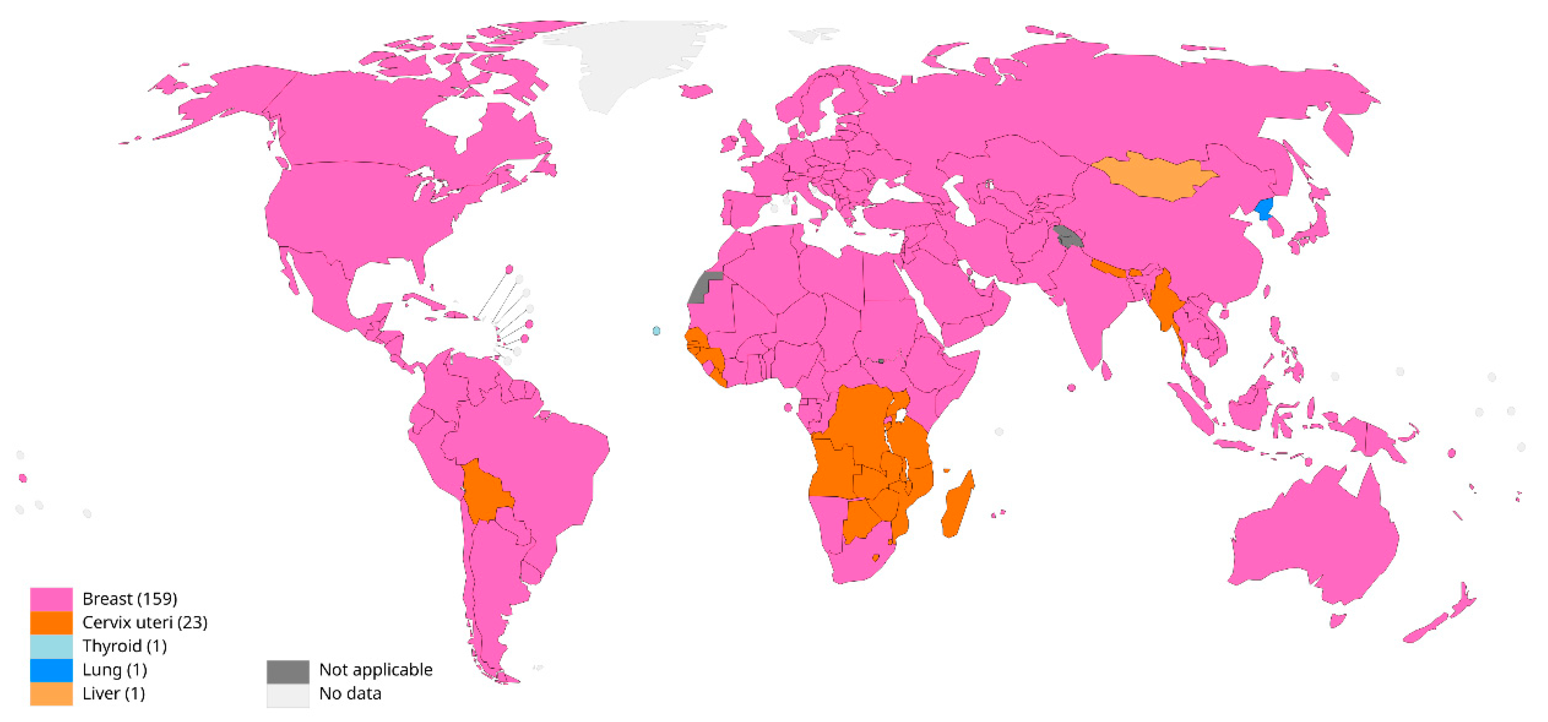
Figure 2.
Regional distribution of breast cancer incidence in women worldwide [4]. It shows the estimated age-standardized incidence rates (World) in 2020, breast, females, all ages.
Figure 2.
Regional distribution of breast cancer incidence in women worldwide [4]. It shows the estimated age-standardized incidence rates (World) in 2020, breast, females, all ages.
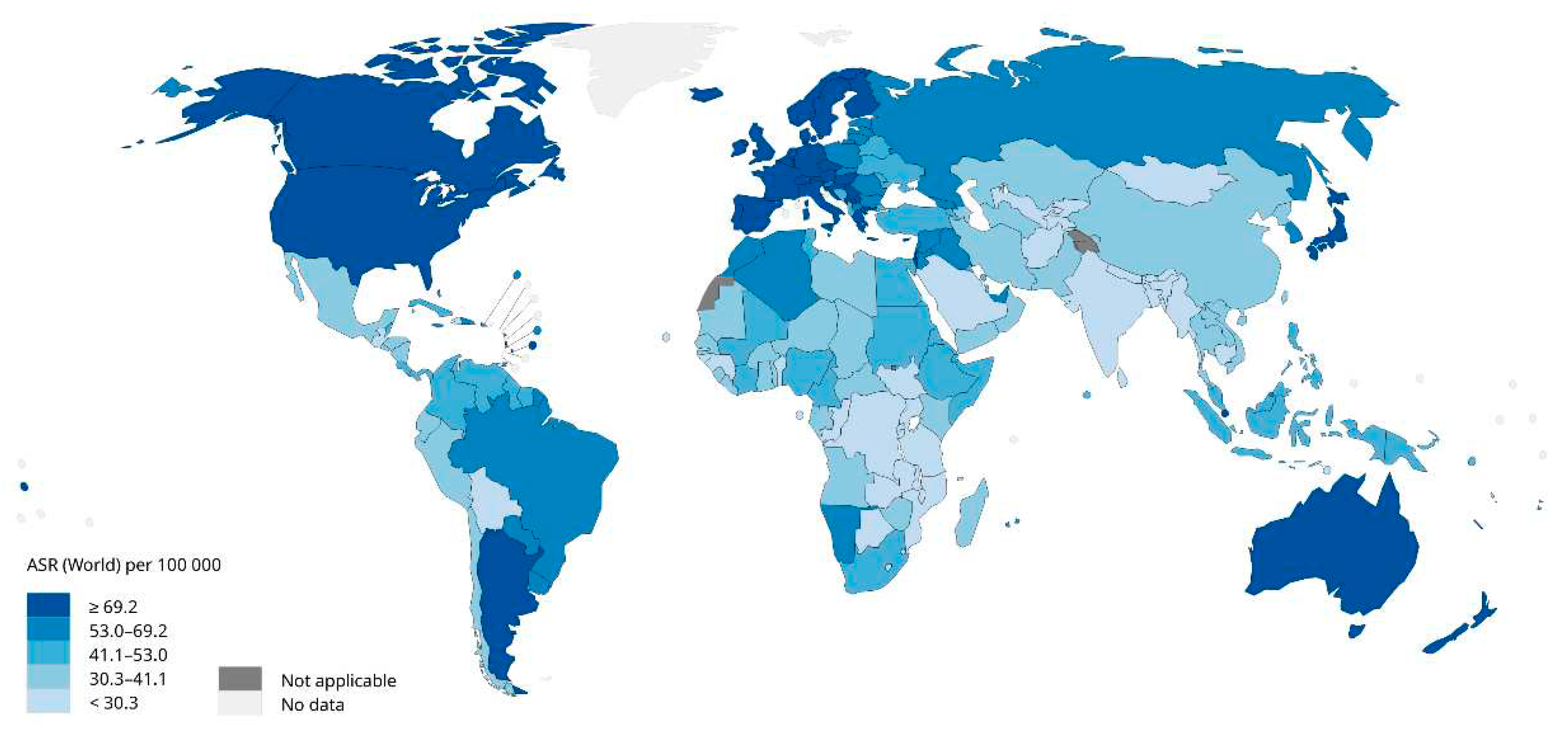
Figure 3.
Visualized results of 729 molecular descriptors.
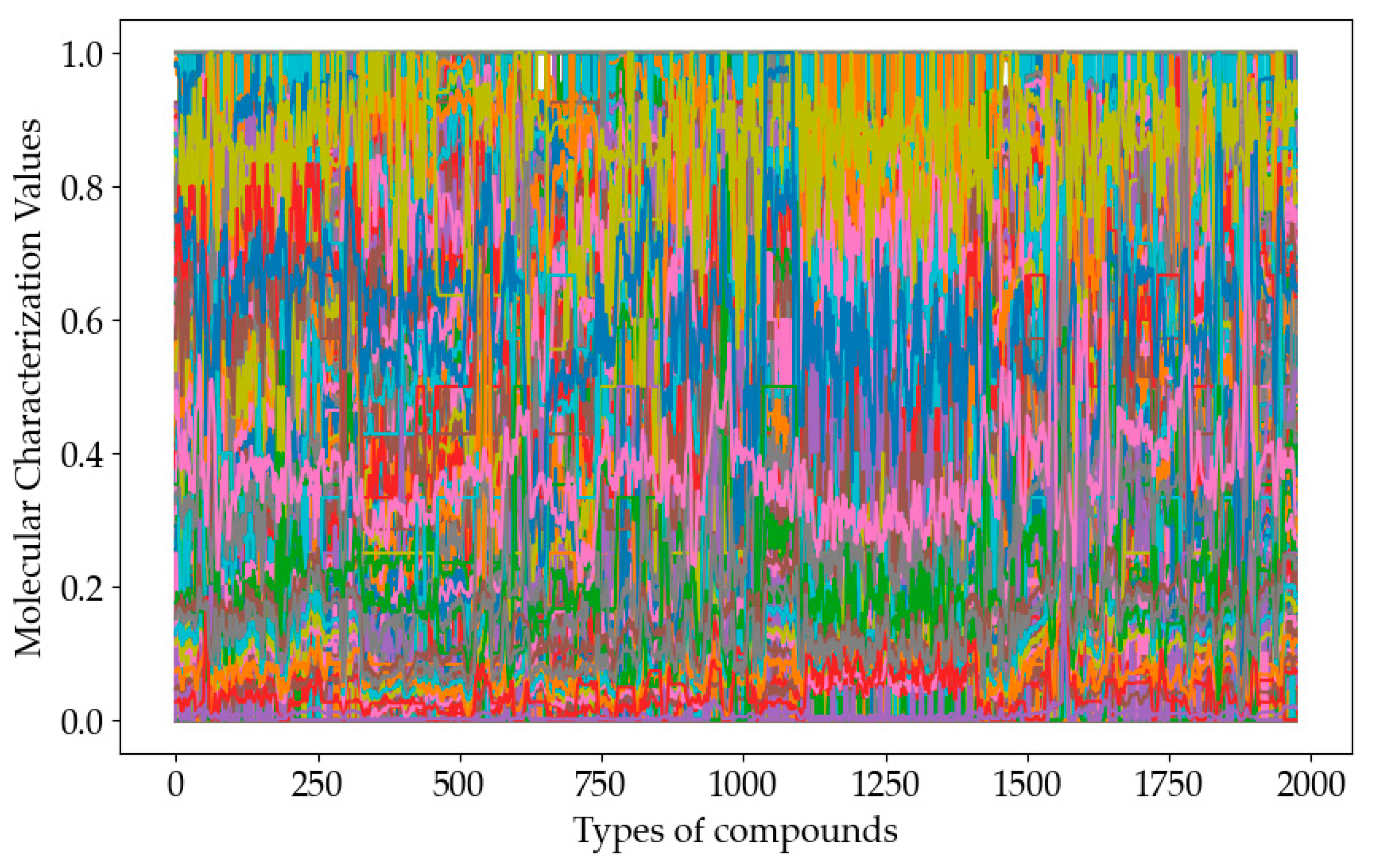
Figure 4.
Box plot of features excluded by Rajda's rule.
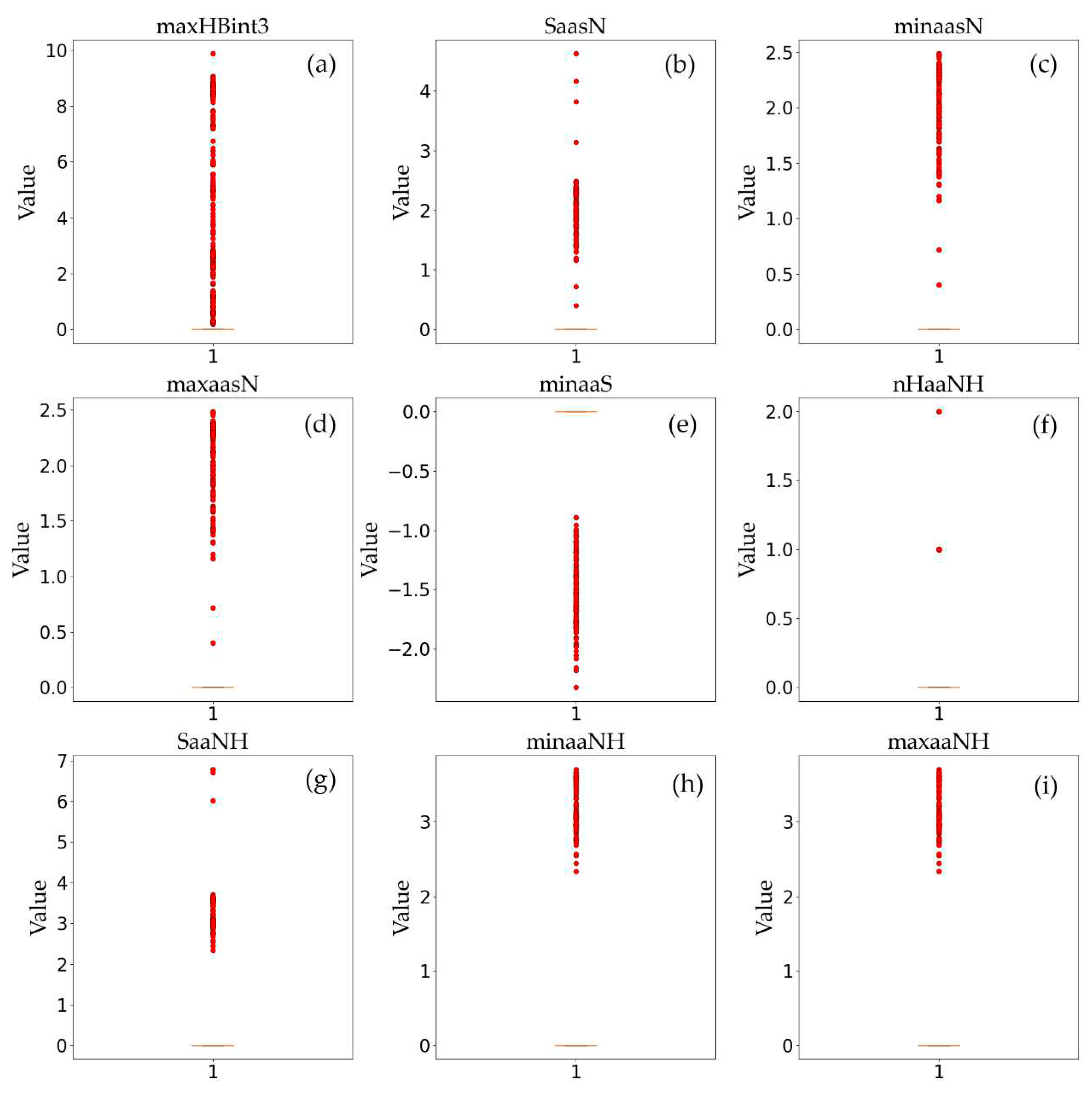
Figure 5.
Schematic diagram of the quantitative prediction model for ERα biological activity.
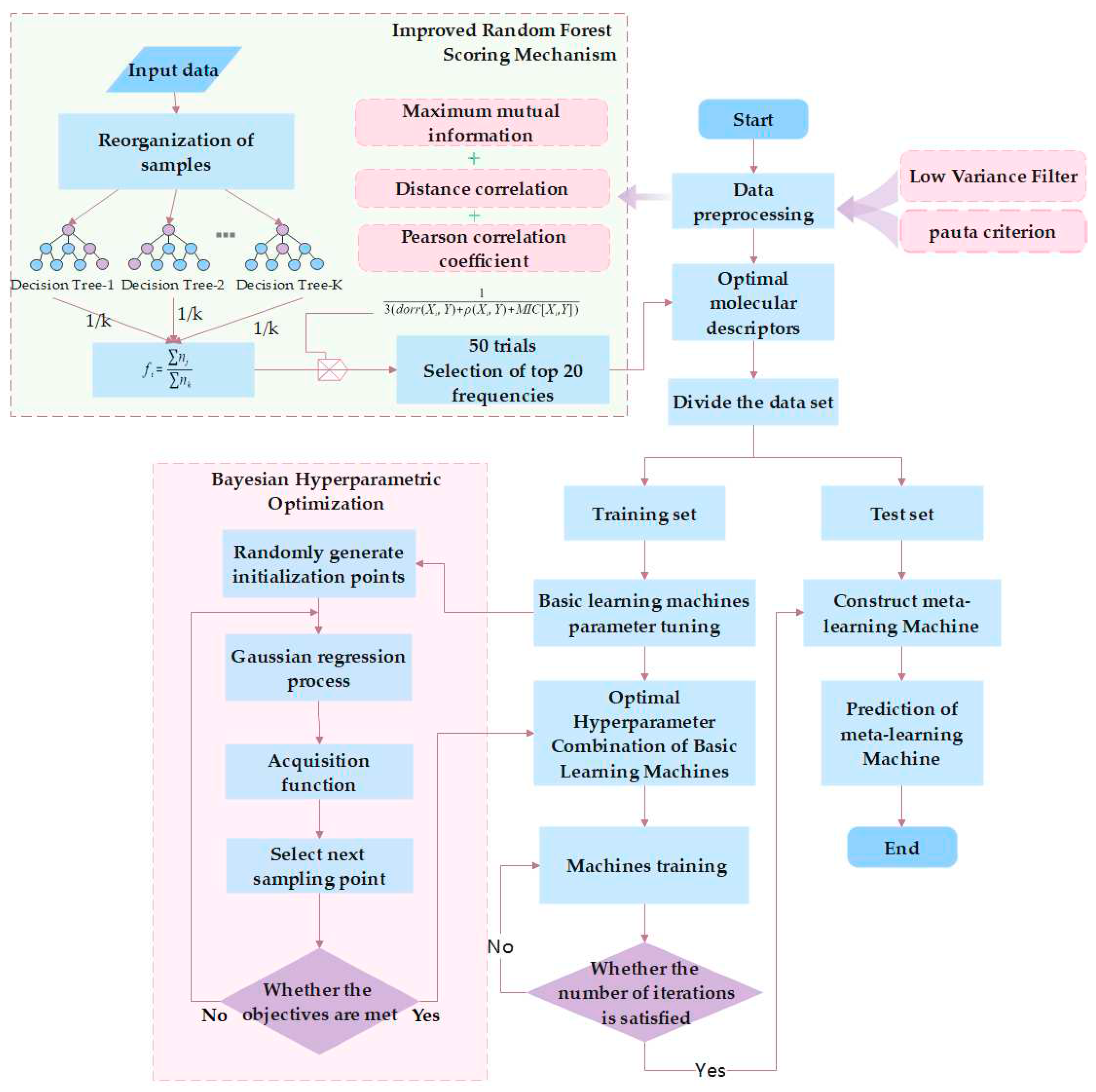
Figure 6.
Framework of the ensemble learning prediction model based on Bayesian hyperparameter optimization (BHO-AdaBoosting).
Figure 6.
Framework of the ensemble learning prediction model based on Bayesian hyperparameter optimization (BHO-AdaBoosting).
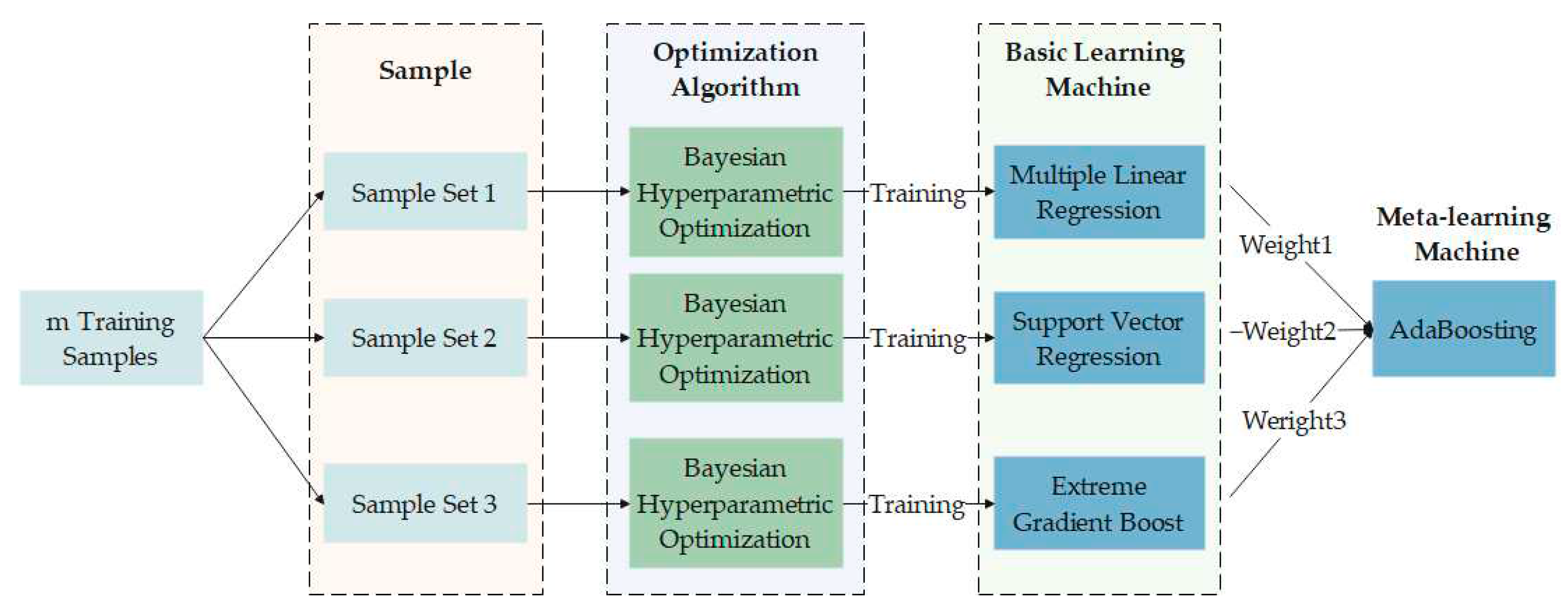
Figure 7.
Figure 7. Diagram of the correlation analysis of the 20 selected features.
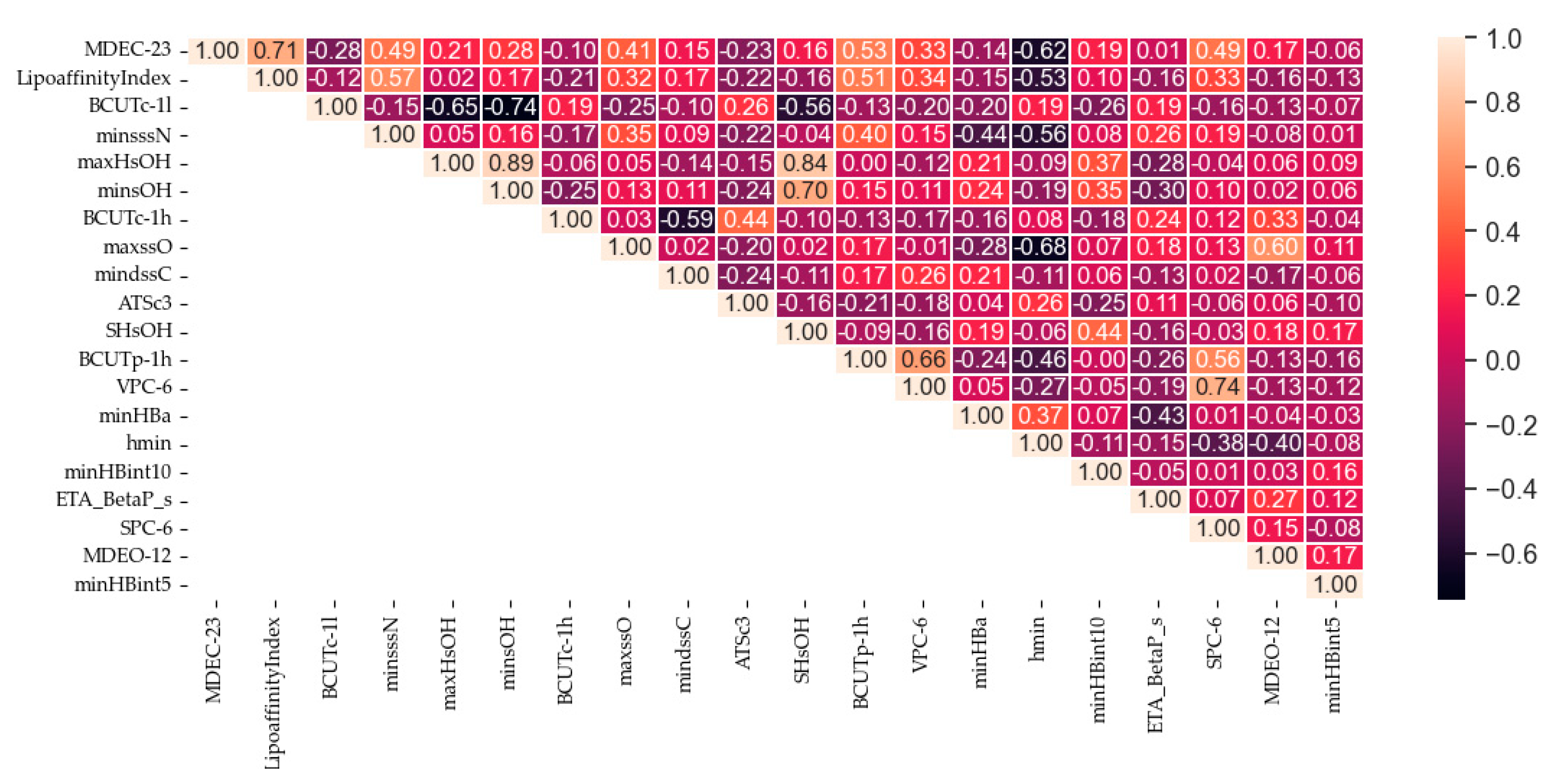
Figure 8.
Comparison of Predicted and Actual Values.
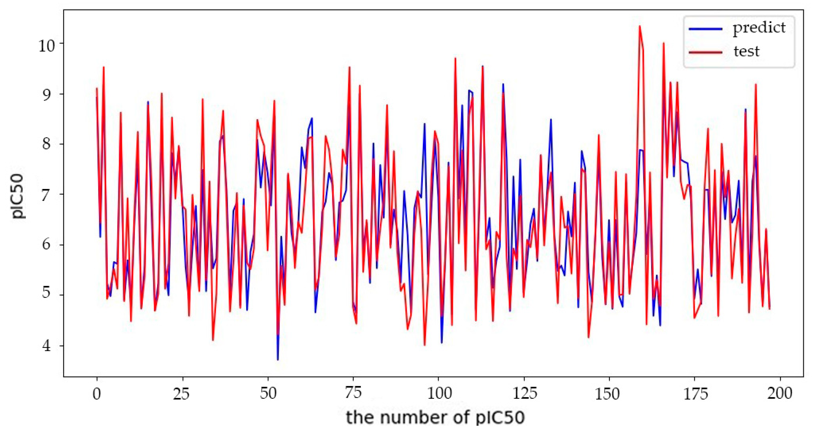
Figure 9.
Comparison of the prediction results of the model test set.
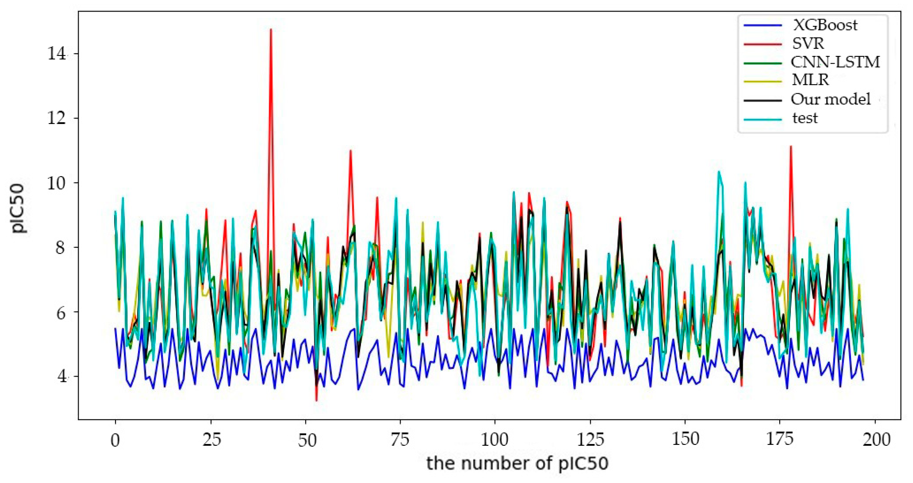
Figure 10.
Distribution of prediction error values for different models.
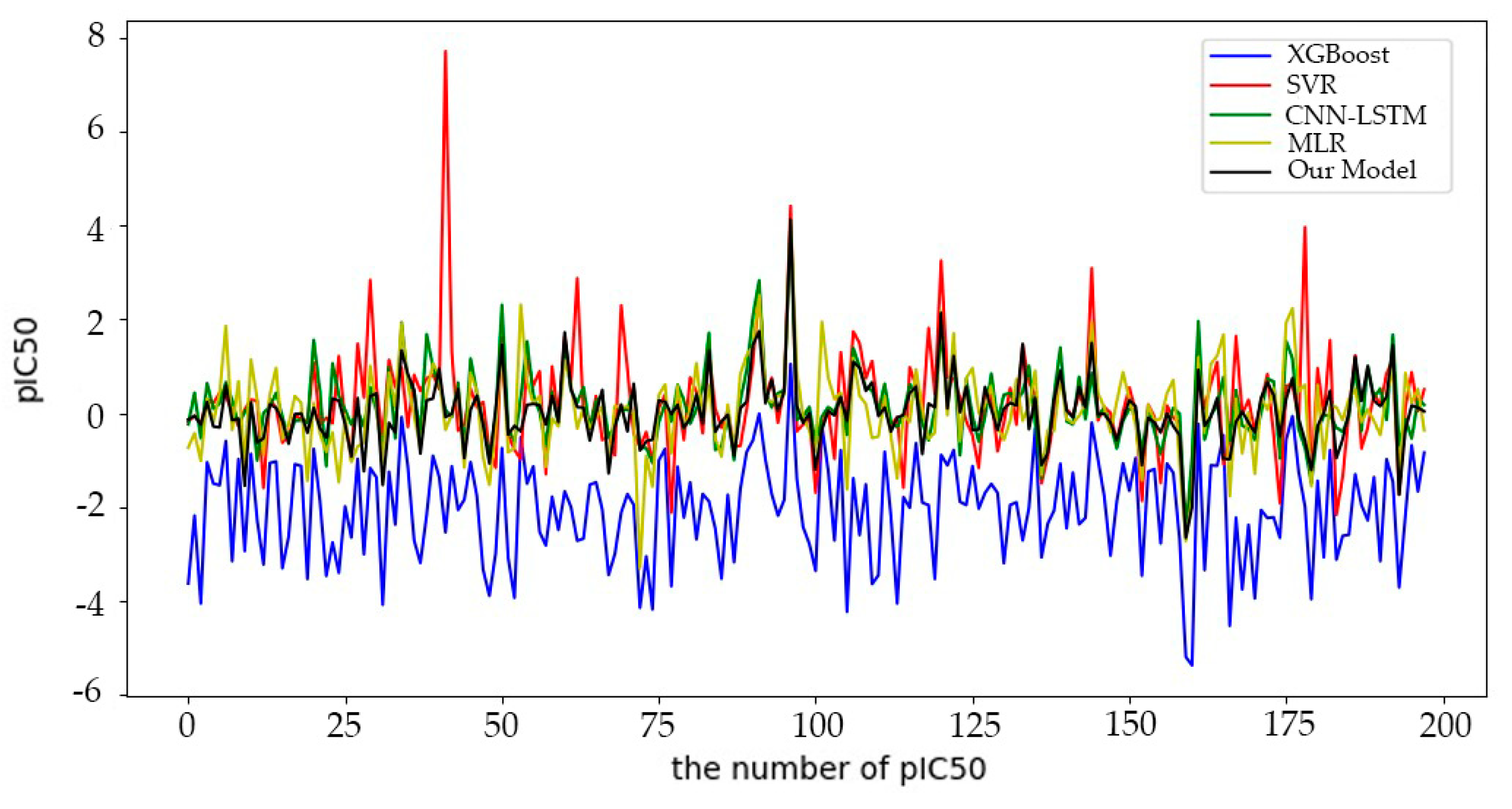

Table 1.
Descriptive statistics of the partial results (N=1974).
| Molecular descriptor | Minimum value | Maximum value | Mean value | Standard deviation |
|---|---|---|---|---|
| pIC50 | 2.456 | 10.34 | 6.59 | 1.42 |
| nAcid | 0.00 | 4.00 | 0.11 | 0.35 |
| ALogP | -23.11 | 5.18 | 1.11 | 1.43 |
| ALogp2 | 0.00 | 533.84 | 3.29 | 12.83 |
| AMR | 54.07 | 517.43 | 116.56 | 31.57 |
| . | . | . | . | . |
| . | . | . | . | . |
| . | . | . | . | . |
| WPATH | 349.00 | 301690.00 | 2709.62 | 7194.53 |
| WPOL | 14.00 | 230.00 | 46.28 | 13.29 |
| XLogP | -3.59 | 14.28 | 2.97 | 1.62 |
| Zagreb | 6.00 | 748.00 | 150.72 | 41.45 |
Table 2.
Screening Results of Characteristic Variables.
| Ranking | Feature name | Contribution degree | Ranking | Feature name | Contribution degree |
|---|---|---|---|---|---|
| 1 | MDEC-23 | 0.3578 | 11 | SHsOH | 0.0281 |
| 2 | LipoaffinityIndex | 0.0802 | 12 | BCUTp-1h | 0.0259 |
| 3 | BCUTc-1l | 0.0761 | 13 | VPC-6 | 0.0247 |
| 4 | minsssN | 0.0548 | 14 | minHBa | 0.0214 |
| 5 | maxHsOH | 0.0530 | 15 | hmin | 0.0210 |
| 6 | minsOH | 0.0406 | 16 | minHBint10 | 0.0203 |
| 7 | BCUTc-1h | 0.0371 | 17 | ETA_BetaP_s | 0.0190 |
| 8 | maxssO | 0.0355 | 18 | SPC-6 | 0.0178 |
| 9 | mindssC | 0.0287 | 19 | MDEO-12 | 0.0152 |
| 10 | ATSc3 | 0.0282 | 20 | minHBint5 | 0.0146 |
Table 3.
Meanings and Ranges of the Base Learner Hyperparameters.
| Model | Hyperparameter | Meaning | Range |
|---|---|---|---|
| XGBoost | n_estimators | Decision tree quantity | [50,100,150,200] |
| max_depth | Maximum depth of the tree | (1,10)evenly distributed, step size is 1. | |
| learning_rate | Learning rate | (10-6,1)logarithmically uniform distribution. | |
| subsample | Ratio of subsamples to training samples | (0.5,1)evenly distributed. | |
| Colsample_bytree | Feature sampling rate | (0.5,1)evenly distributed. | |
| MLR | fit_intercept | Whether to fit the intercept | [True, False] |
| SVR | C | Regularization parameter | (10-6,1)logarithmically uniform distribution. |
| gamma | Kernel value range | (10-6,1)logarithmically uniform distribution. | |
| kernel | Kernel type | ['linear', 'rbf'] |
Table 4.
Parameter settings of the comparison models.
| Model | Parameter setting |
|---|---|
| MLR | default parameter |
| SVR | kernel='rbf', C=1e3, gamma=0.1 |
| XGBoost | objective='reg:squarederror', colsample_bytree=0.3, |
| learning_rate=0.1, | |
| max_depth=5, | |
| alpha=10 | |
| n_estimators=10 | |
| CNN-LSTM | a 1D convolutional layer was established that receives input features of 64 size and holds hidden states of 50 size. |
Table 5.
Prediction performance metrics for different models.
| Model | RMSE | MAE | R2 |
|---|---|---|---|
| MLR | 0.9416 | 0.7002 | 0.5955 |
| SVR | 1.1727 | 0.7698 | 0.3726 |
| XGBoost | 1.9316 | 1.6702 | 0.1591 |
| CNN-LSTM | 0.7486 | 0.5171 | 0.7443 |
| BHO-AdaBoosting | 0.6920 | 0.4837 | 0.8155 |
Table 6.
Activity prediction results for 50 candidate compounds.
| Ranking | MF | pIC50 | Ranking | MF | pIC50 |
|---|---|---|---|---|---|
| 1 | C25H22O3 | 8.583 | 26 | C24H19FO5 | 6.890 |
| 2 | C25H19FO3S | 7.953 | 27 | C51H67N3O10 | 6.885 |
| 3 | C29H33NO2 | 7.859 | 28 | C29H34N2O4 | 6.878 |
| 4 | C31H24FNO3 | 7.733 | 29 | C65H107N21O16 | 6.871 |
| 5 | C36H33FN2O3 | 7.708 | 30 | C65H107N21O16 | 6.871 |
| 6 | C34H30O8S | 7.602 | 31 | C23H17FO3 | 6.854 |
| 7 | C36H33FN2O3 | 7.583 | 32 | C26H23FO5 | 6.847 |
| 8 | C29H27FN2O3 | 7.527 | 33 | C65H107N21O16 | 6.826 |
| 9 | C27H30NO4 | 7.510 | 34 | C64H105N21O16 | 6.822 |
| 10 | C26H22O5 | 7.435 | 35 | C32H34O4 | 6.808 |
| 11 | C30H29FN2O3 | 7.401 | 36 | C62H105N21O16 | 6.764 |
| 12 | C31H23FO3 | 7.384 | 37 | C19H26OS | 6.757 |
| 13 | C30H23FO2 | 7.380 | 38 | C63H101N19O17 | 6.723 |
| 14 | C25H20O4 | 7.348 | 39 | C18H24OS | 6.690 |
| 15 | C31H33FN2O3 | 7.344 | 40 | C27H21FO4 | 6.541 |
| 16 | C29H28FNO3 | 7.327 | 41 | C22H31NO3 | 6.494 |
| 17 | C25H19FO4 | 7.326 | 42 | C21H29NO3 | 6.343 |
| 18 | C29H26FNO3 | 7.239 | 43 | C28H26ClN3O3 | 6.289 |
| 19 | C31H38N2O5 | 7.144 | 44 | C29H28ClN3O3 | 5.978 |
| 20 | C52H71N3O10 | 7.135 | 45 | C26H25ClN4O2 | 5.686 |
| 21 | C26H21FO3 | 7.106 | 46 | C23H26ClN3O3 | 5.544 |
| 22 | C25H22O6 | 7.054 | 47 | C21H22ClN3O3 | 5.411 |
| 23 | C29H33NO2 | 7.048 | 48 | C23H24ClN3O3 | 5.396 |
| 24 | C16H12Cl2M2O2 | 6.969 | 49 | C23H24ClN5O2 | 5.386 |
| 25 | C31H38N2O4 | 6.911 | 50 | C23H27ClN4O2 | 5.358 |
Disclaimer/Publisher’s Note: The statements, opinions and data contained in all publications are solely those of the individual author(s) and contributor(s) and not of MDPI and/or the editor(s). MDPI and/or the editor(s) disclaim responsibility for any injury to people or property resulting from any ideas, methods, instructions or products referred to in the content. |
© 2023 by the authors. Licensee MDPI, Basel, Switzerland. This article is an open access article distributed under the terms and conditions of the Creative Commons Attribution (CC BY) license (http://creativecommons.org/licenses/by/4.0/).
Copyright: This open access article is published under a Creative Commons CC BY 4.0 license, which permit the free download, distribution, and reuse, provided that the author and preprint are cited in any reuse.


