
Submitted:
11 August 2023
Posted:
14 August 2023
You are already at the latest version
Abstract
The internal wave recognition algorithm in an ocean data buoy system can be used to realize the real-time and flexible observation of internal waves, but there is no accurate automatic recognition method. To meet the need for automatic, real-time, and reliable internal wave recognition, an automatic internal wave recognition algorithm has been proposed for a tightly profiled intelligent buoy system. The sea profile temperature data collected by the Bailong buoy system in the Andaman Sea in 2018 were used to train and test the internal wave recognition neural network model, which consists of two parts: feature extraction and feature classification. The experiment compares the long short-term memory network (LSTM), convolutional neural network (CNN) with different layers, and deep neural network (DNN) without a feature extraction network and adjusts the number of convolutional nuclei and convolutional strides to improve the feature extraction efficiency. Experiments show that the best results can be obtained when a CNN layer is used as the feature extraction network, the convolutional step length is 4, the number of convolutional kernels is 5. The recall reaches 95.31% and the precision is 97.53%. The internal wave identification delay of the algorithm is 5.0862 minutes, the number of parameters is 1593, and the number of calculations is 3024. The algorithm can be directly deployed to the ocean data buoy system to realize the demand for automatic, real-time and reliable internal wave identification at the buoy end.
Keywords:
Internal wave recognition
; automation
; CNN
; feature extraction
1. Introduction
Internal waves are an ocean phenomenon with short periods and large amplitudes that can usually reach tens to hundreds of meters [1]. Internal waves have been observed in many sea areas [2,3,4,5,6,7,8]. Internal waves usually occur in the deep ocean and can change the thermohaline structure of seawater by affecting the vertical mixing of seawater, which is an important link in the transfer of large-scale and mesoscale motion energy [9,10]. The impact of internal waves on marine ecosystems is also important. One important impact is that on the supply of nutrients in the upper ocean [11], which is of great significance for ocean productivity and the construction of food chains. In addition, internal waves can also affect the suspension and reaccumulation of seabed sediments, as well as the distribution and transformation of biological and chemical substances in the seabed [12]. Internal waves also affect the species composition, community structure and productivity of some marine ecosystems. Internal waves are also closely related to ocean utilization and maritime activities. Internal waves can affect the navigation of underwater vehicles and the operation of offshore drilling platforms [13] and may also affect the dynamic response of offshore platforms. Therefore, understanding the characteristics and distribution of internal waves and studying their impact on the ocean and the environment are of great significance for understanding the ocean, protecting the environment and improving disaster prevention and reduction.
At present, internal wave recognition methods based on satellite remote sensing images [14,15,16,17,18] and ocean profile data are commonly used [19,20,21]. The satellite remote sensing image method can be used to recognize internal waves by observing irregular light and dark fringes in images. With the rapid development of artificial intelligence, some scholars have carried out research on automatic internal wave recognition algorithms based on satellite remote sensing images. Celona S et al. [16] used X-band radar to collect remote sensing images and a machine learning algorithm of a support vector machine (SVM) model to classify whether the images contained internal solitary waves or tidal internal waves, realizing the automatic detection and classification of internal waves. Bao S et al. [17] used the target detection method to realize the internal wave automatic recognition method based on SAR remote sensing images. However, the observation range of satellite remote sensing images is usually large, and the satellite orbit is constantly changing, so it is impossible to observe specific areas for a long time. In addition, the observation of satellite remote sensing images is affected by natural factors such as weather and clouds [18], which will also affect the identification and observation of internal waves. and the characteristics of internal waves are easily confused with other features in remote sensing images (vortex, ship wake, wind, waves, etc.) [17].
In recent years, some scholars have performed related research on internal wave recognition based on ocean profile data. Zhang B et al. [19], using the physical process of internal waves driving water particles to fluctuate up and down, proposed a method for calculating the amplitude of internal waves. The feasibility of this method was verified using data collected by a temperature chain installed on a moored buoy. However, this algorithm cannot automatically locate the position of internal waves and cannot be directly applied to automatically identify internal waves at the end of the moored buoy. Suanda S H et al. [20] used a buoy equipped with a thermistor to collect offshore ocean temperature profile data for a month, and the collected temperature data were filtered by differential filtering. Then, the filtered data were compared with threshold values, and values greater than the standard threshold value were judged to be internal waves. Liu B et al. [21] proposed a method of measuring internal waves based on a mobile temperature chain real-time monitoring system that was independently designed to perform the mobile real-time monitoring of internal waves, and the method was tested on a monitoring ship. However, through experimental verification, this study found that the recognition effect of the threshold method was not excellent: the recall was 83.33%, the precision was 89.74%, and the delay was 5.2444 minutes.
Deploying the internal wave recognition algorithm to the ocean data buoy system can allo researchers to improve the efficiency of data processing and analysis, reduce the cost of data transmission and processing, improve the real-time performance of observation data, and flexibly respond to different observation situations. However, none of the above methods [19,20,21] can meet the needs of accurate and automatic identification of internal waves in ocean data buoy systems. To solve this problem, an automatic internal wave recognition algorithm for tight buoy ends is designed in this paper. The algorithm can be directly deployed to the end of the buoy. By processing and analyzing the ocean profile temperature data collected by the buoy, the internal wave sign is extracted, and internal wave recognition is carried out by combining the neural network. The algorithm has the characteristics of real-time performance, high reliability and automation and can meet the needs of internal wave recognition of intelligent buoys. In addition, considering the high energy consumption requirement of the buoy end, the algorithm can improve the feature extraction efficiency, reduce the number of parameters and calculation amount of the algorithm, and reduce the energy consumption of the buoy end by selecting a suitable number of convolution kernels and convolution interval.
2. Methods and Materials
2.1. Methods
In this paper, an internal wave recognition algorithm suitable for tight buoys is designed based on a neural network. The neural network algorithm used in the algorithm consists of two modules: a feature extraction module and a feature classification module. The algorithm first uses 1D-CNN [22,23] to extract features from input data and then uses a fully connected neural network to classify features.
2.1.1. Feature extraction module
CNNs can be divided into 1D-CNNs, 2D-CNNs, and 3D-CNNs according to input data types, and CNNs can extract more effective information from much data [24]. The network structure is shown in Figure 1. The original data are a temperature sequence with 14 layers of length 30, which contains 420 feature quantities. After the feature extraction network consisting of 1D-CNN, the data are transformed into a feature sequence with 5 layers of length 8, which contains 40 feature quantities. Feature extraction can be achieved by enlarging the sampling step of the convolution operation and reducing the number of convolution kernels.
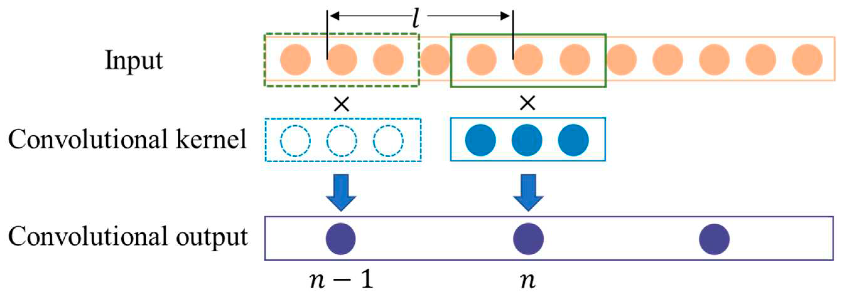
The correlation between adjacent moments of the ocean temperature profile data is strong, so appropriately increasing the sampling stride of the convolution operation will not affect the algorithm. The convolution kernel calculation formula for the ij-th element is shown in formula 1.
where “” refers to the original data, “” represents the convolution output, “” is used to represent the convolution kernel, “” is used to indicate the number of bits that are utilized in the convolution output, “” refers to the sampling step that is used during the convolution operation, and “” represents the length calculation.
From formula 1, the relationship between the input feature number “”, the output feature number “” and the sampling step “” of the convolution operation can be obtained as follows:
Figure 2.
Convolution schematic.
This algorithm identifies internal waves through the temperature data of ocean profiles with multiple depth layers, and the temperature variation trend of adjacent depth layers is similar when internal waves arrive. To solve this problem, this method improves the efficiency of spatial features by designing a suitable number of convolution kernels. The corresponding relationship between and the original data a can be obtained from formula 1, while the output of the feature extraction network is used to calculate the mean value of the convolutional output, as shown in formula 3.
where “” denotes the output of the feature extraction network, “N” refers to the number of layers in the raw data, and “M” represents the number of groups of convolutional kernels.
Formula 3 shows that the spatial dimension of the feature extraction output is related to the number of convolution kernel groups and has nothing to do with the spatial dimension of the original data. Therefore, this method improves the effectiveness of spatial features by testing different numbers of convolution kernel groups.
2.1.2. Feature classification module
The feature recognition network of this algorithm is composed of two layers of a fully connected neural network, which does not have the feature extraction capability itself but only performs a nonlinear combination of features [25]. After the output layer, a softmax layer is added to calculate the probability of a category belonging. The softmax expression used in this algorithm is shown in formula 4.
In the formula, output represents the output of the neural network, and and represent the two nodes of the output layer. The of the classification network is a 1×2 matrix, where and are the probabilities of identifying no and yes internal waves, respectively.
Finally, the prediction results and loss function are shown in formulas 5 and 6.
In the formula, represents the prediction result, and indicate that the real label is no internal wave and there is an internal wave, respectively, represents the judgment probability, and represents the loss rate between the algorithm recognition result and the real result.
2.2. Materials
2.2.1. Collection of data
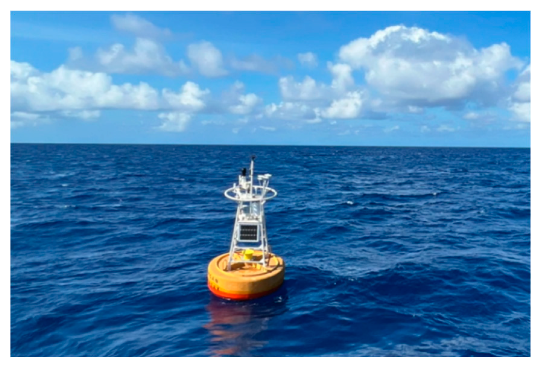
The Bailong buoy [26,27] was independently integrated and developed by the First Institute of Oceanography of the Ministry of Natural Resources. The buoy device consists of a buoy body, an anchor system, a power supply unit, a meteorological sensor, a hydrological sensor and data acquisition control and communication units, as shown in Figure 3. Through comparison and testing with the ATLAS and TFLEX buoys of the United States, the results show that all the data of the Bailong buoy have excellent performance [28]. The temperature profile data of the Bailong buoy placed at 9.6°N and 96°E in the Andaman Sea in the Indian Ocean on December 24, 2018, were used in this experiment. It was continuously observed for 11 months and 17 days and recovered on November 10, 2019.
Figure 3.
Bailong buoy structure diagram.

Figure 4.
The Bailong buoy is located at N and E longitude in the Andaman Sea, Indian Ocean.
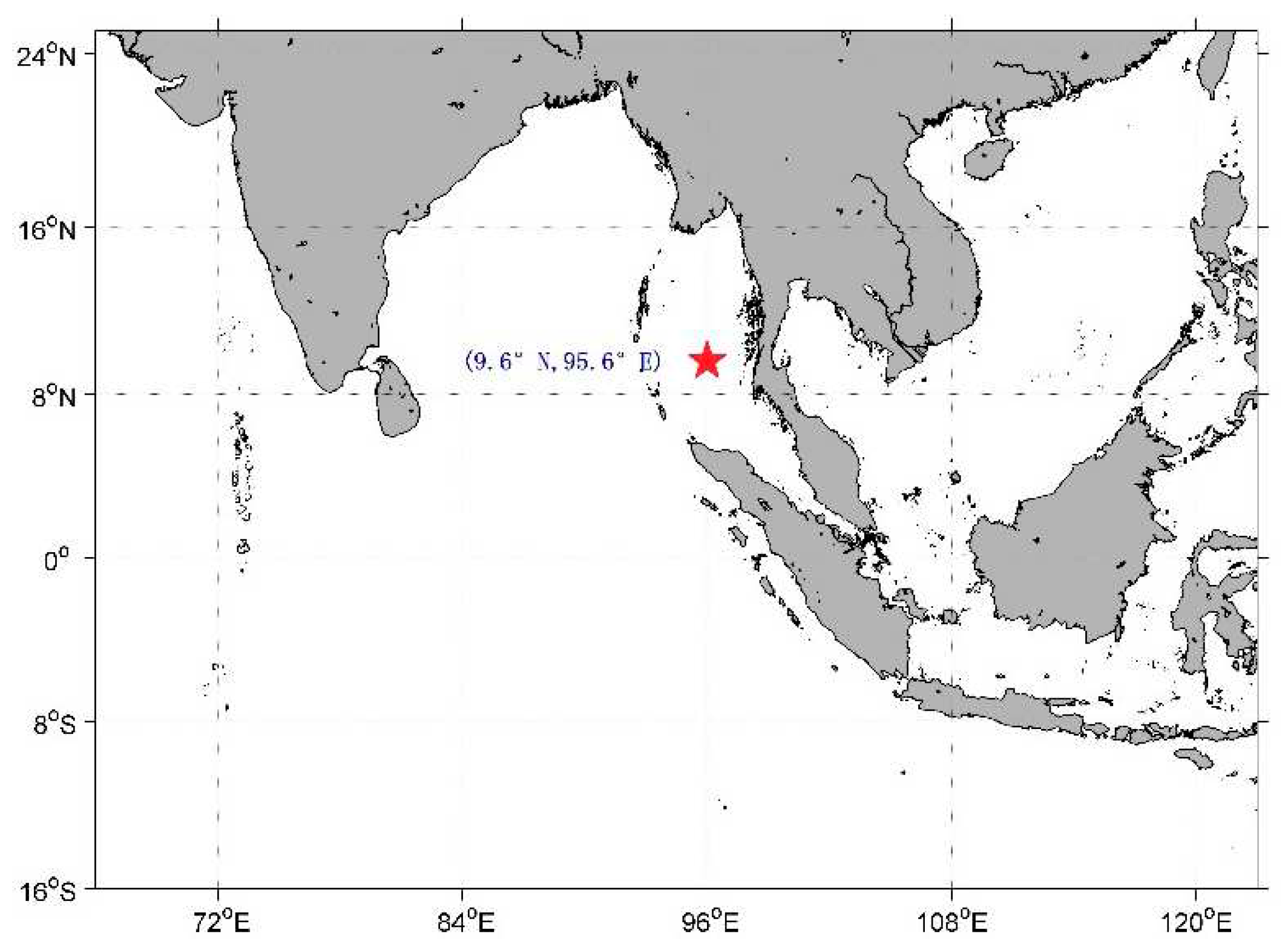
Figure 5.
Observation map of the Bailong buoy from December 24, 2018, to November 10, 2019.
A total of 18 layers of self-contained RBR sensors are installed on the buoy anchorage (layout location is shown in Table 1). The sensor types include T, CT and CTD. The sensor sampling frequency is set to 1 minute, and the layout depth is 0-600 m, among which 0-200 m sensors are dense and 200-600 m sensors are sparse.
2.2.2. Filtering data
According to the collected data, the ocean temperature profile is drawn. As shown in Figure 6, when the water depth is less than 200 m, the temperature changes significantly with increasing water depth, while when the water depth is greater than 200 m, the temperature does not change significantly with increasing water depth. This paper reflects the existence of internal waves through the change in the vertical distribution of water temperature. Therefore, the data of 14 layers of sensors are selected as the data to identify internal waves, in which the sensor layout depth is 15 m, 20 m, 30 m, 40 m, 50 m, 60 m, 70 m, 80 m, 100 m, 120 m, 140 m, 160 m, 180 m, 200 m, 250 m. The selected sensor is mainly concentrated at 40 m-200 m, and the coverage depth of the sensor is appropriately expanded.
2.2.3. Making a data set
The schematic diagram of the vertical SST profile is drawn as shown in Figure 7. The internal waves are marked according to the amplitude and slope of the isotherm [29], and each internal wave start time, extreme time and end time are marked. Finally, the labeling results are compared and revised manually, and a total of 1639 internal wave passing periods are marked by this method.
The labeled data set is divided into three parts: a training set, verification set and test set. The training set and verification set train the neural network, and the test set evaluates the performance of the final network model. The buoy collection data from 2018.12.14-2019.01.24 are taken as the test set, and the buoy collection data from 2019.01.24-2019.11.09 are taken as the training set and verification set. The division ratio of the training set and verification set is 8:2.
3. Experimental preparation
3.1. Experimental evaluation
In this paper, recall (formula 7), precision (formula 8), F1 Score (formula 9) and delay (formula 10) are used as metrics of the internal wave recognition algorithm. Recall is used to measure the model's ability to identify internal waves. Precision is used to measure the accuracy of model recognition of internal waves. Generally, recall and precision are expected to both be high, but in some cases, the two indicators are contradictory. Therefore, the F1 score is used to reconcile recall and precision. In addition, the difference between the time when internal waves are recognized and the start time when internal waves are marked is defined as the delay. As shown in Table 2, the presence of internal waves is defined as a positive object, while the absence of internal waves is defined as a negative object.
In the formula, indicates the number of samples that are correctly classified as having internal waves, indicates the number of samples that are correctly classified as having no internal waves, and indicates the number of samples that are incorrectly classified as having internal waves. represents the number of samples incorrectly classified as nonexistent internal waves. represents the internal wave identified position, and represents the internal wave start position marked in the data set.
In addition, to explore the effectiveness of the feature extraction network, in addition to the above evaluation indicators of the algorithm, this paper also compares the data correlation and the number of features (N) before and after feature extraction. Finally, to study the practicability of the algorithm, we calculate the storage cost and computing cost using different model structures, in which the storage cost is measured by the model parameter number (Parameters) index, and the computing cost is measured by the floating-point number (FLOPs) index.
3.2. Experimental environment
In this study, all the experimental code source code is Python, using the PyTorch neural network architecture; the software installation version is Python 3.8.10, torch 1.11.1, cuda11.3. The computing unit uses an RTX2080Ti graphics card with 11 GB video memory and 40 GB RAM.
4. Verification algorithm
4.1. Reliability verification
To compare the artificial intelligence method with the threshold method [19,20], the threshold method used in this study uses the same test set as the artificial intelligence method to identify internal waves. The threshold method determines the range of temperature changes within 30 minutes by setting a threshold (θ) to determine whether there is an internal wave. The effects of different thresholds on the experiment are shown in Table 3.
When the threshold recognition internal wave method is set at 2.5, the recall rate is close to 100%, but the precision is close to 45.49%. As increases, recall decreases sharply, precision increases sharply, and delay becomes longer. When , the precision is 97.65%, but the corresponding recall is only 65.87%, and the delay reaches 8.2759 minutes. Therefore, the threshold method cannot balance the relationship between recall and precision, and the reliability of the algorithm cannot be guaranteed in practical applications.
Compared with the threshold method, the recognition effect of the artificial intelligence method has been significantly improved, as shown in Figure 8. The feature extraction network can extract and strengthen the internal wave signs and delete irrelevant features. The feature recognition network is trained to fit the internal wave sign through historical data, which takes more internal wave sign elements into consideration and has a better recognition effect than the threshold method neural network. From the experimental results, the recall reaches 95.31% precision, and the 97.53% Magi delay drops to 5.0862 minutes; therefore, while precision is improved, recall is kept at a high level, which greatly improves the reliability of the algorithm in practical applications.
To further verify the reliability of the artificial intelligence algorithm used in this paper, the artificial intelligence algorithm and threshold method are compared with the actual internal wave temperature vertical structure observation data, in which it is specified that the period when internal waves are recognized is a low state, and the period when internal waves are not recognized is a high state. The comparison results are shown in Figure 9. Compared with the threshold method, the artificial intelligence method can identify more internal waves, as shown in Fig. 9(A) and Fig. 9(B). Due to the slow temperature change rate, the threshold method cannot identify these internal waves. In addition, the artificial intelligence method has fewer misidentification phenomena, as shown in Fig. 9(C) and Fig. 9(D). The threshold method has misidentification phenomena, which is caused by the fact that although the temperature in the misidentification period tends to rise or fall, it is not enough to define this period as an internal wave period. Artificial intelligence algorithms can improve the accuracy and reliability of internal wave recognition by extracting and identifying internal wave signs.
4.2. Validity verification of the feature extraction network
In this paper, by adjusting the convolution stride and the number of convolution kernels of the feature extraction network, the effectiveness of features is improved in the time dimension and space dimension, respectively. The internal wave recognition effect is the best when the convolution stride is 4 and the number of convolution kernels is 5. The feature extraction network has 420 input features and 40 output features, and the efficiency of feature extraction can reach 90.48%. The correlation matrix between the input and output data of the feature extraction network is shown in Figure 10. The correlations between the original data can be reduced through the feature extraction network.
4.2.1. Sampling step selection of convolution operation
To compare the effects of sampling steps of different convolution operations on the experiment, this study compares the effects of convolution steps from 1 to 7 on the results of internal wave recognition. Figure 11 shows that when the convolution step amplitude changes from 1 to 4, the changes in recall, precision, F1 Score and delay are not obvious, but when the stride continues to increase, F1 Score will have a significant downward trend, and delay will have an obvious prolongation trend because the collected underwater temperature profile series is a continuously collected time series, and increasing the sampling interval by properly increasing the convolution step has little effect on the final internal wave recognition results. However, when the convolution step is raised to 5, the internal wave recognition has an obvious downward trend, so this method selects a convolution step of 4 to sample the sequence, and when the number of convolution cores is 8, the output feature number is 64, as shown in Table 4.
4.2.2. Selection of the number of convolution kernels
To reduce the spatial information redundancy of the input data, this paper selects the appropriate number of convolution kernels to obtain more effective spatial features for internal wave recognition. The number of convolution kernels selected in the experiment is 1-9. When the number of convolution kernels is 1, it is found that the algorithm does not converge, and when the convolution kernel is 2-9, the experimental results are shown in Figure 12. When the number of convolution kernels increases from 2 to 3, the recognition effect of the algorithm is not obvious. When the number of convolution kernels is increased from 3 to 5, the recognition effect of the algorithm is significantly improved. When the number of convolution kernels is raised from 5 to 9, it is found that the internal wave recognition effect is not improved, so the final number of convolution kernels selected by this algorithm is 5, and the number of output features is 40 when the convolution step is 4, as shown in Table 5.
4.3. Practical verification
By comparing the recognition results of different network structures, the one-layer convolutional neural network plus fully connected internal wave recognition network used in this paper has the best result. Figure 13 shows the precision-recall curve of various methods, in which the precision-recall curve of this method is significantly higher than that of other network structures. As shown in Table 6, the effect of internal wave recognition is significantly improved after adding the feature extraction network, and the effect of the feature extraction network using one-dimensional convolution is also better than that of other feature extraction networks. This method has an F1 score that is 3.4% higher than that of the F1 score without the feature extraction network structure. The delay has been shortened by 1.22 minutes, and compared with the two-layer CNN and three-layer CNN feature extraction network structure, the F1 score has been improved by 2.46% and 2.14%, respectively, and the delay is shorter by 0.53 min and 1.09 min, respectively,. The delay is shorter by 0.5 min compared with LSTM and the F1 Score is increased by 2.12%.
In terms of the calculation of the number of network parameters, because this method reduces the input features of the feature recognition network by selecting the appropriate convolution steps and the number of convolution kernels, the number of parameters and computation of the algorithm are greatly reduced. As shown in Table 7, the number of parameters and the amount of calculation of this method are 1593 and 3024, respectively. Compared with the direct feature recognition method, the number of parameters is reduced by 88.2%, and the amount of calculation is reduced by 77.66%.
According to the analysis of the recognition effect of the algorithm, the number of parameters and the amount of calculation, the algorithm has a good recognition effect, fewer parameters and less calculation. The parameters and FLOPs of the algorithm are 1593 and 3024, respectively, so it requires very low storage capacity and computing power of the equipment. The algorithm can be directly deployed in the controller of the intelligent buoy to meet the needs of automatic recognition of internal waves at the buoy end.
5. Conclusion
This paper proposes an automatic internal wave recognition algorithm applicable to ocean data buoys. The reliability and practicability of the proposed algorithm, as well as the effectiveness of the feature extraction network, are verified using the training set, verification set and test set, which were originally taken from the Bailong buoy data. The conclusions are as follows:
- 1)
- It is found through experiments that the threshold method cannot balance the two parameters of recall and precision, but both recall and precision can be improved to more than 95% by the method based on CNN, in which recall can reach 95.31% and precision is 97.53%. Compared to the threshold method, the recall and precision of the CNN-based method are improved by 11.98% and 7.79%, respectively, which meets the requirement of accurate identification of internal waves at the buoy end.
- 2)
- The feature extraction network based on CNN is introduced in this algorithm, and the optimal number of convolutional cores and convolutional strides are selected through experiments, which improves the efficiency of the feature extraction network and reduces the calculation amount and parameter number of the algorithm. Among them, the feature extraction efficiency reaches 90.48%, with 1593 algorithm parameters and 3024 algorithm computations.
- 3)
- Through a comparison with other network model structures, it is found that this algorithm has a good recognition effect and low requirements for computation and storage. The proposed algorithm can be directly deployed into the ARM-based controller of the intelligent buoy to achieve the requirements of automatic and reliable recognition of internal waves at the ocean data buoy system.
Acknowledgments
This work was supported by the National Key Research and Development Program of China (Grant No. 2022YFC3104301).
References
- Alford, M. H. , Peacock, T., Mackinnon, J. A., et al,2015. The formation and fate of internal waves in the South China Sea. Nature.521:65-69. [CrossRef]
- Alford, M. H. , Cronin, M. F., et al,2012. Annual Cycle and Depth Penetration of Wind-Generated Near-InertiaI Internal Waves at Ocean Station Papa in the Northeast Pacific. Journal of Physical Oceanography. 42(6), p.889-909. [CrossRef]
- Puig, P. , Palanques, A., et al,2004. Role of internal waves in the generation of nepheloid layers on the northwestern alboran slope: implications for continental margin shaping. Journal of Geophysical Research Oceans.109(C9). [CrossRef]
- Orr, Marshall, H, 2003. Nonlinear internal waves in the South China Sea: Observation of the conversion of depression internal waves to elevation internal waves. Journal of Geophysical Research Oceans.108(C3), -. [CrossRef]
- Quaresma, L. S. , Vitorino, J., Oliveira, A., et al,2007. Evidence of sediment resuspension by nonlinear internal waves on the western portuguese mid-shelf. Marine Geology.246(2-4), 123-143. [CrossRef]
- Wong, S. H. C. , Santoro, A. E., Nidzieko, N. J., Hench, J. L., et al,2012. Coupled physical, chemical, and microbiological measurements suggest a connection between internal waves and surf zone water quality in the southern california bight. Continental Shelf Research. 34(none), 64-78. [CrossRef]
- A, J. C. B. D. S. , B, M. C. B., & A, J. M. M., et al,2015. Internal waves on the upstream side of a large sill of the mascarene ridge: a comprehensive view of their generation mechanisms and evolution. Deep Sea Research Part I: Oceanographic Research Papers. 99, 87-104. [CrossRef]
- Qiu, B. , Nakano, T., Chen, S., et al,2017. Submesoscale transition from geostrophic flows to internal waves in the northwestern pacific upper ocean. Nature Communications. 8, 14055. [CrossRef]
- Wijesekera, H. W. , Teague, W. J., Jarosz, E., et al,2019. Internal tidal currents and solitons in the southern bay of bengal. Deep Sea Research Part II: Topical Studies in Oceanography, 168, 104587-. [CrossRef]
- A, Tommy. G. Jensen., et al,2019. Numerical modelling of tidally generated internal wave radiation from the andaman sea into the bay of bengal. Deep Sea Research Part II: Topical Studies in Oceanography. 172. [CrossRef]
- Hirawake, T. , Kawaguchi, Y., Onodera, J., et al,2015. Nutrient supply and biological response to wind-induced mixing, inertial motion, internal waves, and currents in the northern chukchi sea. Journal of Geophysical Research, C. Oceans: JGR. [CrossRef]
- Diamessis, P. J. , Jacobs, G. B.,2015. Near-Bottom Turbulence and Sediment Resuspension Induced by Nonlinear Internal Waves. Cornell University Ithaca NY.
- Moore, S. E. , Lien, R. C, 2007. Pilot whales follow internal solitary waves in the South China Sea. Marine mammal science, 23(1), 193-196. [CrossRef]
- [14] Zhang, X. , Wang, H., Wang, S., Liu, Y., Yu, W., Wang, J., Xu, Q., Li, X., 2022. Oceanic internal wave amplitude retrieval from satellite images based on a data-driven transfer learning model. REMOTE SENSING OF ENVIRONMENT. 272. [CrossRef]
- [15] Zhang, X. , Li, X.,2022. Satellite data-driven and knowledge-informed machine learning model for estimating global internal solitary wave speed. REMOTE SENSING OF ENVIRONMENT. 283. [CrossRef]
- Celona, S. , Merrifield, S. T., et al,2021. Automated detection, classification, and tracking of internal wave signatures using X-band radar in the inner shelf. Journal of Atmospheric and Oceanic Technology, 38(4), 789-803. [CrossRef]
- Bao, S. , Meng, J., Sun, L., et al,2020. Detection of ocean internal waves based on Faster R-CNN in SAR images. Journal of Oceanology and Limnology, 38(1), 55-63. [CrossRef]
- Shen, H. , Li, X., et al, 2015. Missing information reconstruction of remote sensing data: A technical review. IEEE Geoscience and Remote Sensing Magazine, 3(3), 61-85. [CrossRef]
- Zhang, B. , Chen, W., Chen, B., et al,2014. Observation of the amplitude of internal waves in the South China Sea using the temperature chain. Journal of Ocean University of China (Natural Science Edition),44(07): 24-28. [CrossRef]
- Suanda, S. H. , Barth, J. A., et al.2014. Shore-based video observations of nonlinear internal waves across the inner shelf. Journal of Atmospheric and Oceanic Technology, 31(3), 714-728. [CrossRef]
- Liu, B. , 2022.Research on measurement method of internal wave based on mobile temperature chain real-time monitoring system. Wireless Internet Technology, 2022, 19(15):6.
- Wu, H. , Chen, J., Liu, X., et al, 2019. One-dimensional CNN-based intelligent recognition of vibrations in pipeline monitoring with DAS. Journal of Lightwave Technology, 37(17), 4359-4366. [CrossRef]
- León, A. A. S. , Alvarez, J. R. N., 2019. 1D convolutional neural network for detecting ventricular heartbeats. IEEE Latin America Transactions, 17(12), 1970-1977. [CrossRef]
- Raj, S. , Prakasam, P., Gupta, S., 2021. Multilayered convolutional neural network-based auto-CODEC for audio signal denoising using mel-frequency cepstral coefficients. Neural Computing and Applications, 33, 10199-10209. [CrossRef]
- Guo, M. , Li, W., et al. Application of deep convolutional neural network in shaft trajectory recognition of sliding bearing rotor. Vibration and Shock, 40(3), 233-239. [CrossRef]
- Lu, X. , Chen, M., Wang, X., Zhou, Y., et al, 2020. Development history of marine hydrological survey equipment in China. Ocean Development and Management, 37(9):5. [CrossRef]
- Ning, C. , Xue, L., Jiang, L., et al, 2022. The solution of global communication system sharing of Bailong buoy data. Journal of Hehai University (Philosophy and Social Sciences Edition), 050-003. [CrossRef]
- Freitag, H.P. , Ning, C., Berk, P., et al, 2016. Atlax, T-flex, Bailong METEOROLOGICAL sensor comparison test report. NOAA Technical Memorandum OAR PMEL-148.
- Gerkema, T. , 2008.An introduction to internal waves. Lecture Notes, Royal NIOZ, Texel, 207, 207.
Figure 1.
Internal wave recognition network structure diagram.
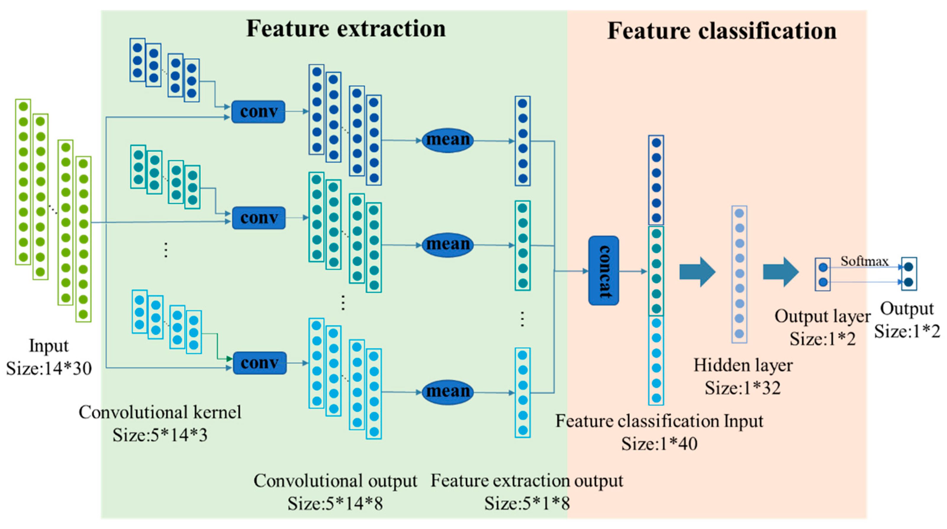
Figure 6.
Diagram of temperature change in ocean profile.
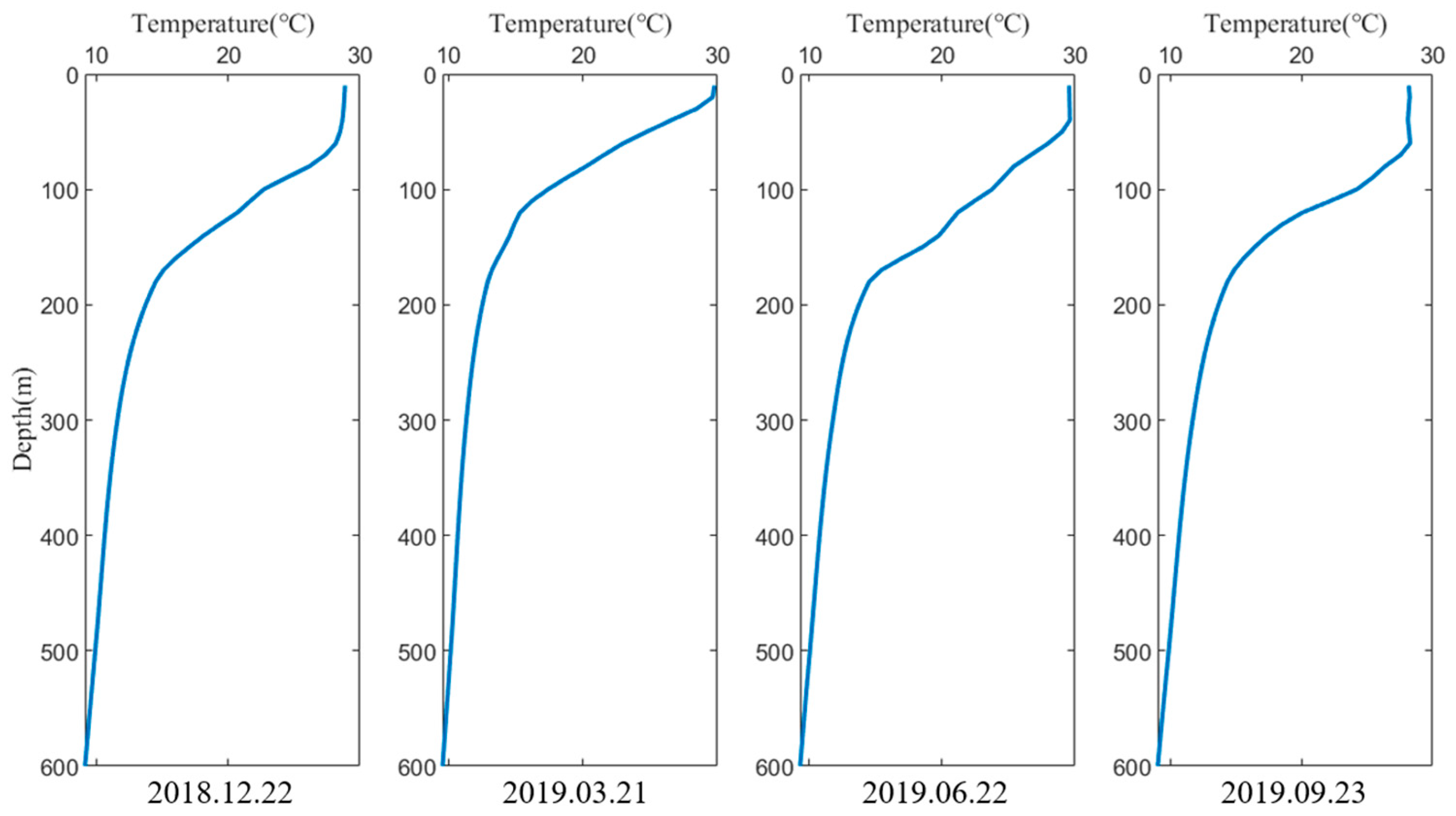
Figure 7.
Schematic diagram of the vertical SST profile observed by buoy.
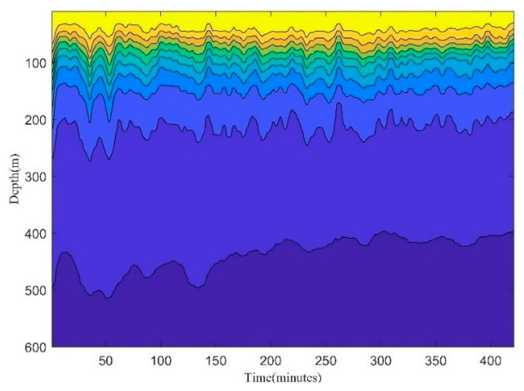
Figure 8.
Comparison chart between the threshold method and artificial intelligence method. Note: The threshold method has the best performance of the F1 score when θ=3, so the experimental results of θ=3 are selected for comparison.
Figure 8.
Comparison chart between the threshold method and artificial intelligence method. Note: The threshold method has the best performance of the F1 score when θ=3, so the experimental results of θ=3 are selected for comparison.
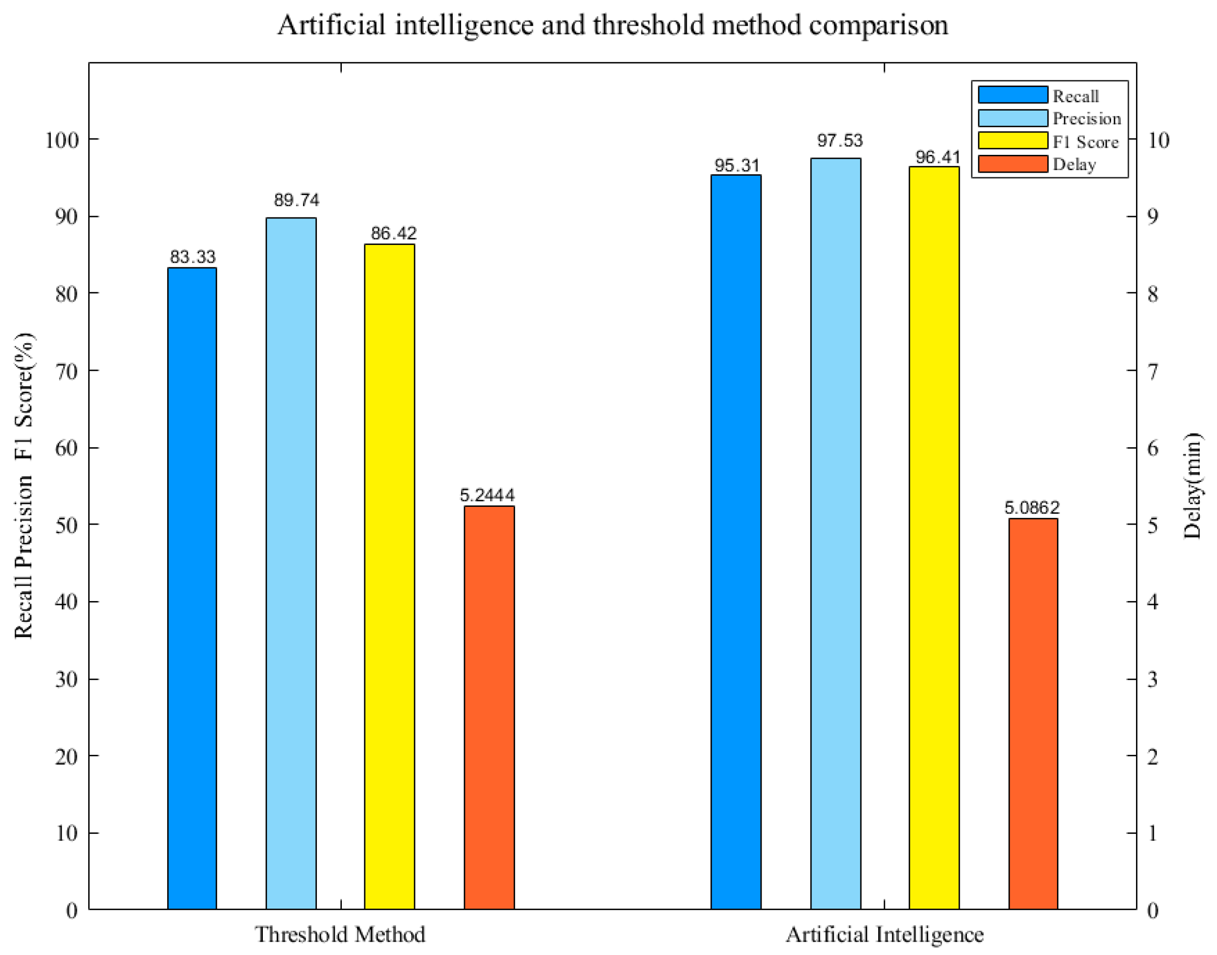
Figure 9.
Threshold method and artificial intelligence method observation comparison graph.
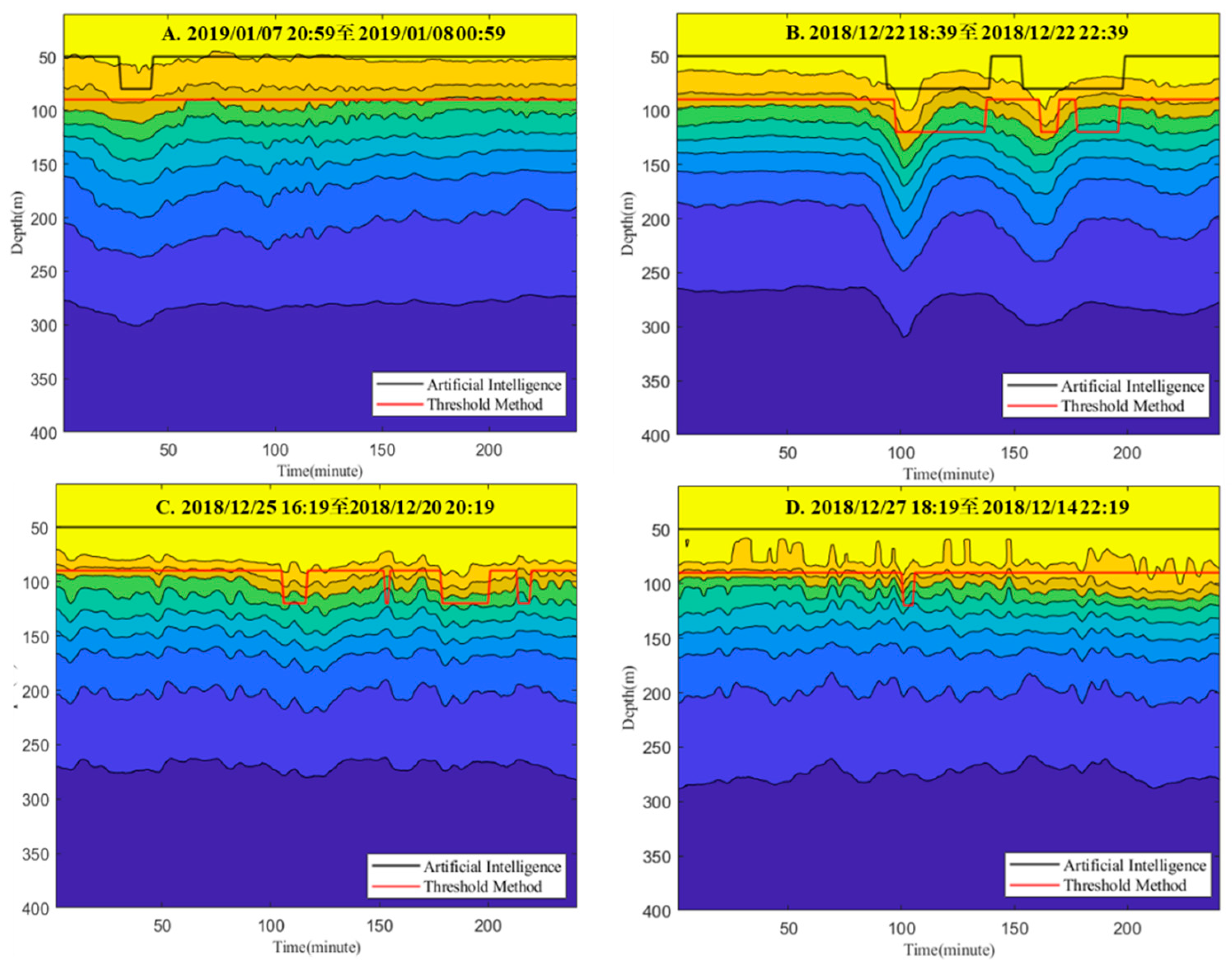
Figure 10.
Comparison of the input‒output correlation matrix of the feature extraction network.
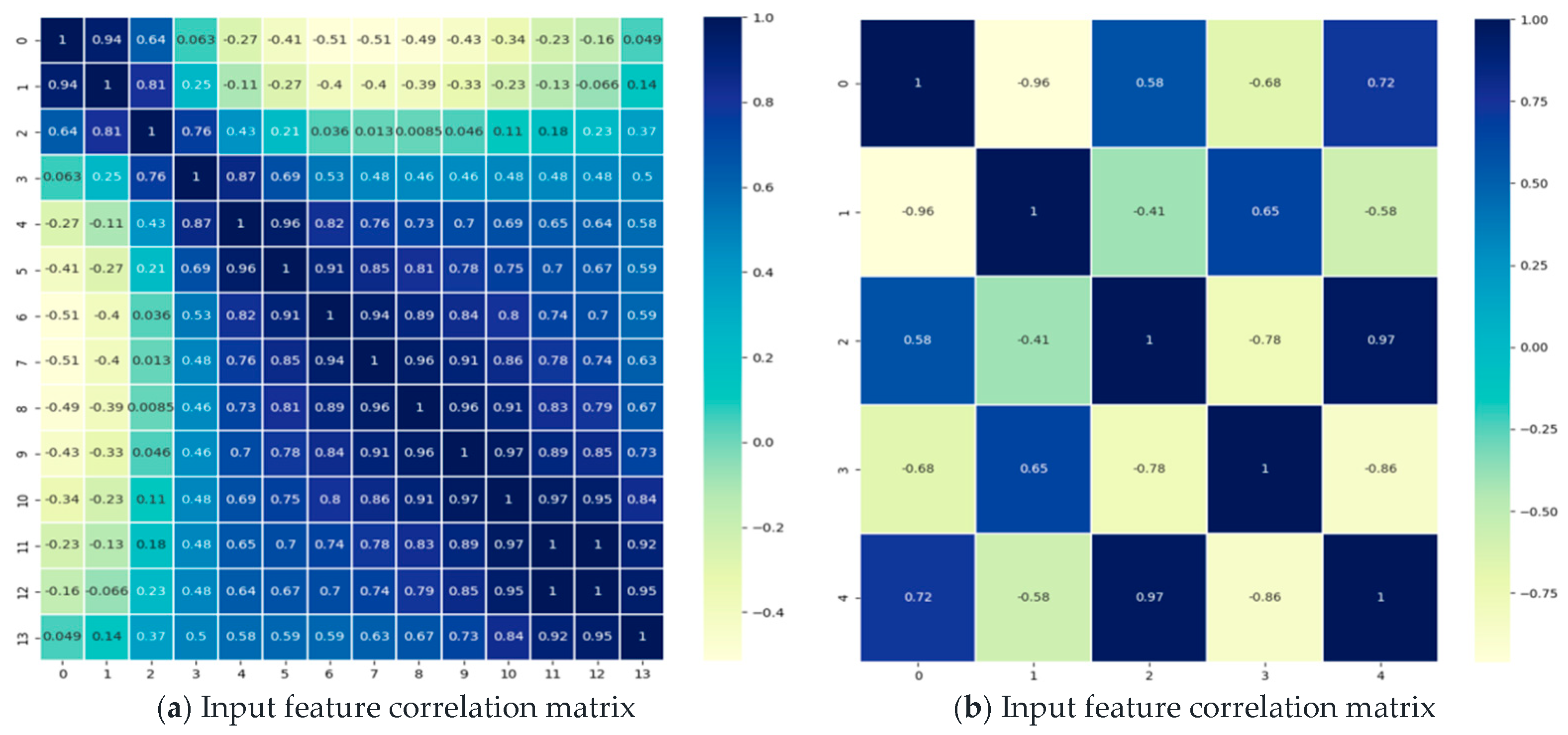
Figure 11.
Influence of the convolution stride of the convolution operation on the result of internal wave recognition.
Figure 11.
Influence of the convolution stride of the convolution operation on the result of internal wave recognition.
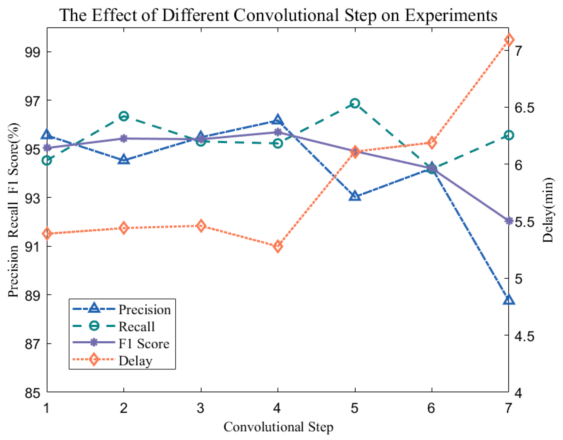
Figure 12.
The influence of the number of convolution kernels on internal wave recognition.
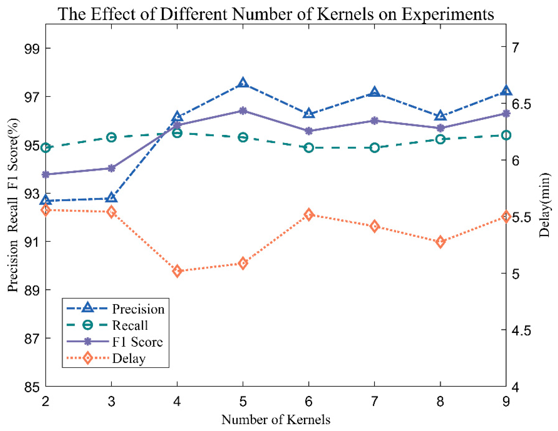
Figure 13.
Precision-recall curve comparison of different networks.
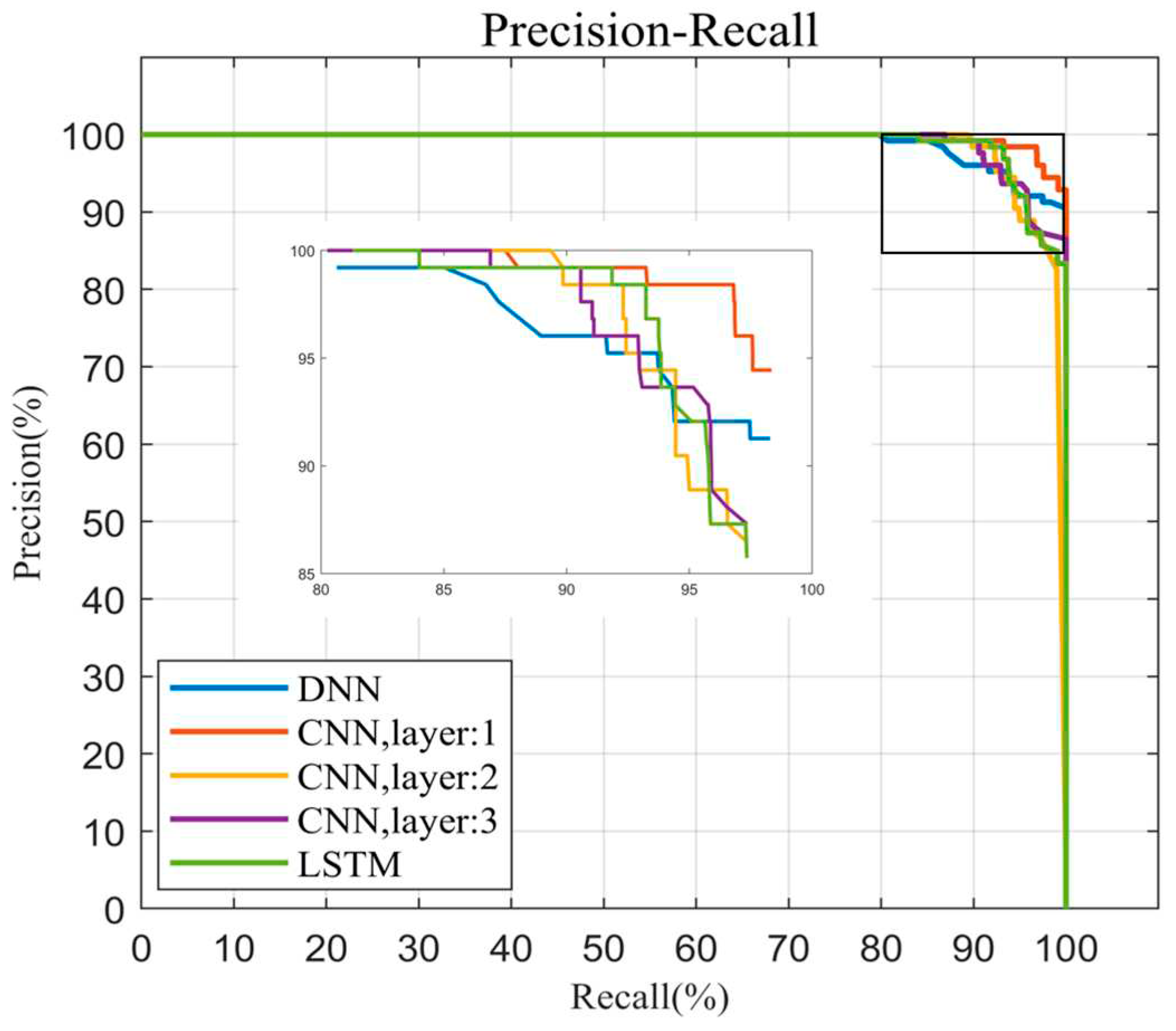

Table 1.
RBR sensor layout position.
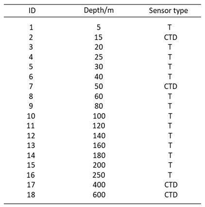 |
Table 2.
Confusion matrix with or without binary classification of internal waves.
| Predict label/True label | Presence of internal wave | No internal waves present |
|---|---|---|
| Presence of internal wave | TP | FP |
| No internal waves present | FN | TN |
Table 3.
Experimental results of the threshold method.
| Recall/% | Precision/% | F1 Score/% | Delay/minutes | |
|---|---|---|---|---|
| 2.5 | 100 | 45.49 | 62.53 | 3.1240 |
| 3 | 96.83 | 64.89 | 77.71 | 4.2696 |
| 3.5 | 91.27 | 77.18 | 83.64 | 4.8218 |
| 4 | 83.33 | 89.74 | 86.42 | 5.2444 |
| 4.5 | 75.40 | 94.06 | 83.70 | 6 |
| 5 | 65.87 | 97.65 | 78.67 | 7.0145 |
Table 4.
The corresponding relationship between the convolution step and the output feature of the feature extraction network.
Table 4.
The corresponding relationship between the convolution step and the output feature of the feature extraction network.
| Convolutional Step | 1 | 2 | 3 | 4 | 5 | 6 | 7 |
|---|---|---|---|---|---|---|---|
| N | 240 | 120 | 80 | 64 | 48 | 40 | 32 |
Table 5.
The corresponding relationship between the number of convolution kernels and the output features of the feature extraction network.
Table 5.
The corresponding relationship between the number of convolution kernels and the output features of the feature extraction network.
| Number of kernels | 2 | 3 | 4 | 5 | 6 | 7 | 8 | 9 |
|---|---|---|---|---|---|---|---|---|
| N | 16 | 24 | 32 | 40 | 48 | 56 | 64 | 72 |
Table 6.
Influence of different network structures on internal wave recognition results.
| Recall (%) | Precision (%) | F1 Score (%) | T (min) | |
|---|---|---|---|---|
| DNN | 0.8845 | 0.9829 | 0.9311 | 6.3084 |
| CNN (layer=1) | 0.9531 | 0.9753 | 0.9641 | 5.0862 |
| CNN (layer=2) | 0.9479 | 0.9313 | 0.9395 | 5.6154 |
| CNN (layer=3) | 0.9627 | 0.9236 | 0.9427 | 5.2137 |
| LSTM | 0.9410 | 0.9449 | 0.9429 | 5.5893 |
Table 7.
Comparison of the number of parameters and computation of different networks.
| Parameters | FLOPs | |
|---|---|---|
| DNN | 13504 | 13538 |
| CNN (layer=1) | 1593 | 3024 |
| CNN (layer=2) | 9250 | 29344 |
| CNN (layer=3) | 10034 | 40864 |
| LSTM | 80704 | 17506 |
Disclaimer/Publisher’s Note: The statements, opinions and data contained in all publications are solely those of the individual author(s) and contributor(s) and not of MDPI and/or the editor(s). MDPI and/or the editor(s) disclaim responsibility for any injury to people or property resulting from any ideas, methods, instructions or products referred to in the content. |
© 2023 by the authors. Licensee MDPI, Basel, Switzerland. This article is an open access article distributed under the terms and conditions of the Creative Commons Attribution (CC BY) license (http://creativecommons.org/licenses/by/4.0/).
Copyright: This open access article is published under a Creative Commons CC BY 4.0 license, which permit the free download, distribution, and reuse, provided that the author and preprint are cited in any reuse.


