
Submitted:
01 August 2023
Posted:
03 August 2023
You are already at the latest version
Abstract
Humans learn from a lot of information sources to make decisions. Once this information is learned in the brain, spatio-temporal associations are made, connecting all these sources (variables) in space and time represented as brain connectivity. In reality, to make a decision, we usually have only part of the infor-mation, either as a limited number of variables, or limited time to make the decision, or both. The brain functions as spatio-temporal associative memory. Inspired by the ability of the human brain, a brain-inspired spatio-temporal associative memory was proposed earlier, that utilizes the NeuCube brain-inspired spiking neural network framework. Here we apply the STAM framework to develop STAM for neuroimaging data, on the cases of EEG and fMRI, resulting in STAM-EEG and STAM-fMRI. The paper shows that once a NeuCube STAM classification model is trained on a complete spatio-temporal EEG or fMRI data, it can be recalled using only part of the time series, or/and only part of the used variables. We evaluate accordingly the temporal association accuracy and spatial association accuracy. This is a pilot study that opens the field for the development of multimodal classification systems on other multimodal neuroimaging data, such as the also shown longitudinal MRI data, trained on complete data, but recalled on partial data collected across different settings, in different labs and clinics, that may vary in terms of variables, time of data collection, and other parameters. The proposed methods will allow also for brain diagnostic/prognostic marker discovery using spatio-temporal neuroimaging data.
Keywords:
spatio-temporal associative memory
; STAM
; neuroimaging data
; spiking neural networks
; NeuCube
; EEG
; fMRI
; neuroimage classification
1. Introduction
Memory is referred to as the brain’s ability to recall experiences or information that is encountered or learnt previously. If this information is recalled using only partial inputs, we refer to it as Associative Memory (AM) [1,2]. There are three main types of memory in the brain, namely sensory memory, short-term or working memory, and long-term memory, which function in different ways, but each of these types are manifested through brain activities in space (areas of the brain) and time (spiking sequences), stored as connection weights and recalled always with only partial input information in time and space. AM in the brain is always spatio-temporal.
Humans can learn and understand many categories and objects from spatio-temporal stimuli by finding spatial and temporal association between them. Inspired by this human brain capability, AM has been introduced to the machine learning field to memorize information and retrieve it from partial or noisy data. For example, neural network models for associative pattern recognition was proposed by J.Hopfield [3] and B.Kosko [4]. In 2019 Haga and Fukai [5] introduced a memory system for neural networks based on an attractor network, which is a group of connected nodes that display patterns of activity and tend towards certain states. They applied the concept of excitatory and inhibitory nodes to their proposed network to mimic the role of hippocampus in balancing network to form new association. The work above related to vector-based data (e.g., static images) and not to spatio-temporal data. None of them related specifically to neuroimaging (NI) data.
The idea of using a brain-inspired and brain-structured spiking neural network (SNN) as a spatio-temporal associative memory (STAM) was first introduced in [6] as part of the NeuCube SNN architecture, but the main concepts and definitions of STAM were introduced in [7], where a NeuCube model, trained on complete spatio-temporal data, creating spatio-temporal patterns in its connections, is recalled when only partial spatio- or/and temporal information is provided as inputs.
In this paper we introduce for the first time STAM on NI data, such as EEG and fMRI. The paper is organized in the following way. Section 2 presents the background concept of STAM from [7]. Section 3 presents a STAM-EEG classification model, while section 4 presents a STAM-fMRI classification model. Section 5 is a conclusion and further discussions towards using the STAM approach across bioengineering applications, including multimodal neuroimaging data.
2. SNN and the STAM-SNN concept from [7]
2.1. Spiking neural networks (SNN)
Spiking neural networks (SNN) are biologically inspired ANN where information is represented as binary events (spikes), similar to the event potentials in the brain, and learning is also inspired by principles in the brain. SNN are also universal computational mechanisms [8,9]. Learning in SNN relates to changes of connection weights between two spatially located spiking neurons over time (Figure 1), so that both “time” and “space” are learned in the spatially distributed connections.
A well-known unsupervised learning paradigm inspired by the Hebbian learning principle is spike-time dependent plasticity (STDP) [8], in which the synaptic weights are adjusted based on the temporal order of the incoming spike (pre-synaptic) and the output spike(post-synaptic). STDP is expressed in (Equation 1), where and are time parameters and and refer to the temporal synaptic adjustment.
2.2. STAM on the NeuCube Framework [7]
The NeuCube architecture is depicted in Figure 2 [6]. It consists of the following functional modules:
- Input data encoding module.
- 3D SNN reservoir module (SNNcube).
- Output function (classification) module, such as deSNN [11].
- Gene regulatory network (GRN) module (optional).
- Parameter optimization module (optional).
Spatio-temporal input data is first encoded into spike sequences and then spatio-temporal patterns of these sequences are learned in a SNNcube that is structured according to a brain temple, such as Talairach [12], MNI [13], personal MRI [14]. Connections are created and strengthened in the SNNcube through DTDP learning. Once data is learned, the SNNcube retains the connections as a long-term memory.
The main trust of the proposed STAM concept in [7] is that, since a SNNcube learns functional pathways of spiking activities represented as structural pathways of connections, when only a small initial part of input data is entered the SNN will ‘synfire’ and ‘chain-fire’ learned connection pathways [15] to reproduce learned functional pathways as polichronisation of neuronal clusters [16]. Some studies defined the state of a SNN as a dynamic chaotic attractor [17] that can be reached with partial input information. In [18,19] polychronous neuronal groups are studied that are activated from partial inputs.
In a STAM model based on NeuCube [7], for every spatio-temporal input sequence Pi, a state Si of the SNNcube is defined as a sequence of activated neurons Si1, Si2, …, SiN over time, that is learned in a deSNN classifier [11], forming an N -element vector Wi of connection weights of an output neuron Oi assigned through supervised learning to the input sequence Pi. When a new input sequence Pnew is presented, either as a full sequence in time and space (number of input variables) or as a partial one, the new SNNcube state Snew is learned as a new output neuron Onew, which weigh vector Wnew is compared with the weight vectors of the existing output neurons for classification tasks or for time series prediction tasks using k-nearest neighbour method. The Pnew is classified based on the output classes (for classification tasks) or the assigned real output values (for prediction tasks) of the closest, according to the Euclidean distance, output weight vectors.
In principle, STAM is a system that is trained for classification or prediction on all available spatio-temporal variables and recalled only on part of the spatial or/and temporal components of the data, without compromising the model accuracy. To validate a STAM model, several types of accuracy tests are introduced in [7]:
- Temporal association accuracy: validating the full model on partial temporal data of the same variables and same data.
- Spatial association accuracy: validation of the full model on full temporal data and on a subset of variables, using the same data set.
- Temporal generalization accuracy: validation of the full model on partial temporal data of the same variables or a subset of them, but on a new data set.
- Spatial generalization accuracy: validation of the full model on full or partial temporal data and on a subset of variables, using a new data set.
The above accuracy tests are applied differently for classification and for prediction tasks [7]. The STAM concept is used in the next subsection to develop specific STAM-EEG (section 3) and STAM-fMRI (section 4).
3. STAM-EEG for classification
3.1. The proposed STAM-EEG classification method
The proposed STAM-EEG classification method, consists of the following steps:
- Defining the spatial and the temporal components of the EEG data for the classification task, e.g., EEG channels and EEG time series data.
- Designing a SNNcube that is structured according to a brain template suitable for the EEG data (e.g., Talairach, or MNI, etc.).
- Defining the mapping in the input EEG channels into the SNNcube 3D structure (see Figure 3a as an example of mapping 14 EEG channels in a Talairach structured SNNcube).
- Encode data and train a NeuCube model to classify a complete spatio-temporal EEG data, having K EEG channels measured over time T.
- Analyse the model through cluster analysis, spiking activity and the EEG channel spiking proportional diagram (Figs. 3b, c,d,e).
- Recall the STAM-EEG model on the same data and same variables but measured over time T1 < T to calculate the classification temporal association accuracy.
- Recall the STAM-EEG model on K1<K EEG channels to evaluate the classification spatial association accuracy.
- Recall the model on the same variables, measured over time T or T1 < T on a new data to calculate the classification temporal generalization accuracy.
- Recall the NeuCube model on K1<K EEG channels to evaluate the classification spatial generalization accuracy using a new EEG dataset.
- Evaluate the K1 EEG channels as potential classification brain biomarkers according to the problem at hand.
3.2. Experimental results
The EEG data consist of 60 recordings of 14 EEG channels of a subject who is moving a wrist: up (class 1), straight (class 2) and down (class 3). The data includes 20 samples for each class, each sample measured as 128 time points used to discretize 1,000ms signal.
The main question to address here is: What will be the classification temporal association accuracy when a trained NeuCube STAM-EEG model on all 60 samples and 14 variables is recalled on a shorter sub-section of time of the same variables and same data? The parameter settings of the STAM-EEG NeuCube model are shown Table 1.
To validate the performance of a NeuCube STAM-EEG model in the realm of associative memory tasks, we initially trained the full model with a complete set of 60 samples (Figure 3a) and analyzed the connectivity and the spiking activity of the model (Figure 3b-e).
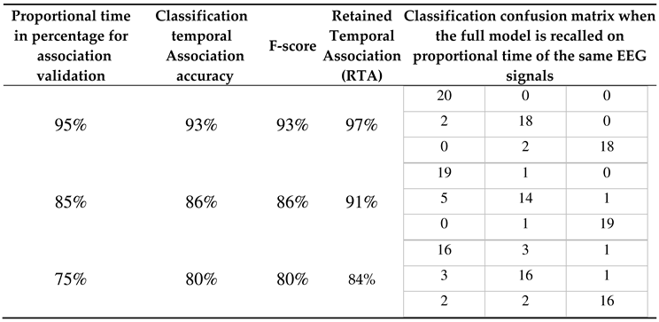
To evaluate the classification temporal association accuracy of the fully trained NeuCube STAM-EEG model from Figs.4a-e, the model was recalled with the same EEG data but on a smaller percentage of time. The validation results are shown in Table 2, along with a new association measurement introduced here, called retained temporal association (RTA) as calculated using Equation. 2 below:
where: Af is the classification accuracy of the full model, validated on the same training data, and Ar is the accuracy of the model validated on the same data, but using shorter time series.
3.3. Why STAM-EEG are needed?
The proposed in this section method STAM-EEG, based on the NeuCube SNN, is illustrated on a simple EEG problem, but its applicability is wide across any studies involving EEG data. A large STAM-EEG system can be developed for a particular problem, involving millions of EEG samples and hundreds of EEG channels, integrating EEG data from different sources and studies. This model can be validated for its temporal and spatial association and generalisation accuracy on a particular sub-set of EEG channels, measured at shorter times. If the validation accuracies are acceptable, then the model can be successfully used on the new EEG data.
In this case, studies that resulted in smaller, but specific data sets, can benefit from the use of larger models on the same problem.
4. STAM-fMRI for classification
4.1. The proposed STAM-fMRI classification method
The proposed STAM-fMRI method consists of the following steps:
- Defining the spatial and the temporal components of the fMRI data for the classification task, e.g., fMRI voxels and the time series measurement.
- Encode data and train a NeuCube model to classify a complete spatio-temporal fMRI data, having K voxel inputs measured over time T.
- Analyse the model through connectivity and spiking activity analysis around the input voxels (Table 3).
- Recall the STAM-fMRI model on the same data and same variables but measured over time T1 < T to calculate the classification temporal association accuracy.
- Recall the STAM-fMRI on K1<K EEG channels to evaluate the classification spatial association accuracy.
- Recall the model on the same variables, measured over time T or T1 < T on a new data to calculate the classification temporal generalization accuracy.
- Recall the NeuCube model on K1<K voxel variables to evaluate the classification spatial generalization accuracy using a new fMRI dataset.
- Evaluate the K1 fMRI voxel variables as potential classification brain biomarkers (section 4.4).
4.2. STAM-fMRI for classification on experimental fMRI data
The fMRI data set was originally collected by Marcel Just and his colleagues at Carnegie Mellon University’s Center for Cognitive Brain Imaging (CCBI) [21]. The fMRI recorded 5,062 voxels from the whole brain volume while a subject was performing a cognitive reading task. In this task, there were two categories of sentences (affirmative and negative) each was remined on the screen for 8 seconds correspond to 16 measured brain images in fMRI. There were a total number of 40 sentences.
A NeuCube STAM-fMRI model is developed for classification of fMRI samples into two classes (class 1: affirmative sentence and class 2: negative sentence). Signal to noise ratio (SNR) feature selection method was applied to the fMRI data to select vital fMRI voxels with a high power of discrimination between the defined classes. As shown in Figure 4a, we selected 20 top important voxels that had SNR values higher than 0.4 threshold. These 20 fMRI voxels from 40 fMRI samples (related to reading 40 sentences) were used as input variables to train STAM-fMRI model for classification. To this end, we defined two sets of experiments as below:
- Experiment 1 (Section 4.2): training and testing the SNN model using the whole space and time information of fMRI dat. The results are shown in Figure 4a-c.
- Experiment 2 (Section 4.3): training the SNN model using the whole space (voxels) and time information of fMRI data but testing the model using a smaller temporal length of fMRI data. The results are shown in Figure 5.
- Experiment 3 (Section 4.4): training the SNN model using the whole space (voxels) and time information of fMRI data but testing the model using a smaller portion of the spatial information (a smaller number of fMRI variables/voxels). The results are shown in Figure 6.
The fMRI data dimension is defined by the maximum value of x, y, and z coordinates of voxels that forms a volume size of 51×56×8. In this dimension, 5062 voxels are captured. Figure 4a shows that 5,062 voxel coordinates are mapped into a 3-dimensional SNNcube. T top-informative voxels selected via SNR are shown in Figure 4b, which are used as input variables to train the SNNcube model. Table 1 shows the brain region of interest (RoI) associated with these top-20 selected fMRI voxels.
Informative voxels are selected using an SNR feature selection from the fMRI data. The voxels were selected due to their SNR values being higher than a threshold= 0.4. The number of of the selected voxels is 20 representing different areas of interest: LT (3), LOPER (3), LIPL (1), LDLPFC (6), RT (2), CALC (1), LSGA (1), RDLPFC (1), RSGA (1), RIT (1), wth the following full names of the area: left temporal lobe (LT); left opercularis (LOPER); left inferior parietal lobule (LIPL); left dorsolateral prefrontal cortex (LDLPFC) and right dorsolateral prefrontal cortex (RDLPFC); calcarine sulcus (CALC); right supramarginal gyrus (RSGA).
In this classification experiment, we employed the same number of samples, temporal and number of variables for both training and testing the SNN model for classification of fMRI samples into affirmative vs negative classes. The model achieved 100% association accuracy. This is shown in Figure 4c.
The trained model is analyzed in terms of connectivity around each of the input voxels, so that the most connected voxels point to most important areas of the brain involved. This is shown in Table 3.
Figure 5a presents three snapshots of deep learning of eight-second fMRI data in a SNNcube when a subject is reading a negative sentence (time in seconds). Figure 5b captures the internal structural pattern, represented as spatio-temporal connectivity in the SNN model trained with eight-second fMRI data streams. The corresponding functional pattern is illustrated in Figure 5c as a sequence of spiking activity of clusters of neurons in a trained SNNcube. The internal functional dimensionality of the SNN model shows that while the subject was reading a negative sentence, the activated cognitive functions were initiated from the Spatial Visual Processing function. Then it was followed by the Executive functions, including decision making and working memory. From there, the Logical and Emotional Attention functions were involved. Finally, the Emotional Memory formation and Perception functions are evoked.
| area | LT | LOPER | LIPL | LOPER | LDLPFC | LOPER | LT | LDLPFC | RT | CALC | |
| Neg | 1.4 | 0.92 | 1.87 | 1.03 | 2.08 | 1.12 | 1.48 | 0.44 | 0.2 | 0.89 | |
| Aff | 0.9 | 0.56 | 1.01 | 0.87 | 1.03 | 0.65 | 0.89 | 0.23 | 0.1 | 0.43 | |
| area | LSGA | LDLPFC | LT | LDLPFC | RT | LDLPFC | LDLPFC | RDLPFC | RSGA | RIT | Avg |
| Neg | 1.84 | 1.03 | 1.9 | 0.45 | 1.1 | 1.26 | 0.56 | 0.19 | 0.43 | 1.4 | 1.7 |
| Aff | 1.04 | 0.68 | 1.1 | 0.17 | 0.8 | 0.24 | 0.22 | 0.11 | 0.32 | 0.9 | 0.6 |
4.3. STAM-fMRI recalled on partial temporal fMRI data
In this experiment, we used the whole spatial and temporal information from the fMRI data to train the SNN model, however, for testing the model, we used a smaller temporal length of data (from 70% to 50% of fMRI timepoints). This is illustrated in Figure 6.
4.4. STAM-fMRI, recalled on partial spatial fMRI data
This section is related to training the SNNcube with all the 40 samples of fMRI data (20 voxels recorded for 8 seconds), while testing the models by recalling it on smaller number of voxel data to evaluate the classification spatial association accuracy. This is illustrated in Figure 7.
4.5. Potential marker discovery from the STAM-fMRI
The trained STAM-fMRI model can be analysed in terms identifying the most activated brain regions related to reading affirmative and negative sentences. Figure 8 demonstrate the distribution of the average connection weights around the input voxels located in the left and right hemispheres of the trained SNN models related to different sentences.
4.6. STAM for longitudinal MRI neuroimaging
STAM systems can be developed for longitudinal MRI data (STAM-longMRI), such as the one used in [21], where 6 years MRI data has been modelled to predict dementia and AD in 2 and 4 years ahead from a large cohort of data. A STAM-longMRI system can be trained on full length of longitudinal MRI data and used to be recalled on a shorter time to predict future events. MRI images are used to preselect regents of interest (RoI), which are consequently measured as longitudinal times series. The RoI are used as input variables/features and are mapped into a SNNcube structured to a brain template according to their 3D coordinates in this template. The measurements are linearly interpolated to make more time points that still preserve the trend of changes in the data over time. This is detected in a SNNcube connectivity through learning and used to create a STAM-longMRI and to test its association and generalisation accuracy over time and over a smaller number of features.
5. Discussions, conclusions, and directions for further research
The potential applications of the STAM-EEG and STAM-fMRI become evident in various fields, including post-stroke recovery prediction, early diagnosis, and prognosis of mild cognitive impairment (MCI) and Alzheimer's disease (AD), as well as depression and other mental health conditions. These applications can leverage neuroimaging techniques such as EEG and fMRI to analyze spatio-temporal patterns of brain activity and make accurate predictions or classifications.
One notable application is in post-stroke recovery prediction. By training the STAM model on neuroimaging data collected from stroke patients, it can learn the spatio-temporal patterns associated with successful recovery. Subsequently, the model can be recalled using only partial neuroimaging variables or timepoints to predict the recovery trajectory of new stroke patients. This capability can assist clinicians in personalized treatment planning and rehabilitation strategies [23,24].
Another application lies in the early diagnosis and prognosis of MCI and Alzheimer's disease. By training the STAM model on longitudinal neuroimaging data, such as EEG and fMRI recordings, from individuals with and without MCI/AD, it can learn the complex spatio-temporal patterns indicative of disease progression. The model can then be utilized to classify new individuals based on their neuroimaging data, enabling early detection and intervention for improved patient outcomes [25,26].
Depression is another mental health condition that can benefit from the STAM systems. By training the model on neuroimaging data, such as resting-state fMRI, from individuals with depression, it can capture the spatio-temporal associations related to the disorder. This trained model can subsequently be used to classify new individuals as either depressed or non-depressed based on their neuroimaging data, aiding in early diagnosis and treatment planning [27].
Furthermore, the STAM systems hold potential for applications in neurodevelopmental disorders, such as autism spectrum disorder (ASD). By training the model on EEG data, it can identify distinctive spatio-temporal patterns associated with ASD, contributing to early diagnosis and intervention [28]. Similarly, the framework can be applied to investigate brain disorders related to aging, such as Parkinson's disease or age-related cognitive decline [29].
By incorporating multimodal spatio-temporal data, including clinical, genetic, cognitive, and demographic information, during the training phase, a STAM model can enable comprehensive analyses. This integration of multiple modalities aims to enhance the model's ability to make accurate predictions or classifications, even when only a subset of the modalities is available for recall. Such a capability can provide valuable insights for personalized medicine, treatment planning, and patient management [30].
One challenge in STAM system design is how it can effectively associate different data modalities during learning, enabling successful recall even when only one modality is available. For instance, can a STAM model learn brain data from synesthetic subjects who experience auditory sensations when they see colors? Addressing this challenge requires leveraging prior knowledge about brain structural and functional pathways, as well as stimuli data and corresponding spatio-temporal data from subjects. Current understanding of structural connectivity and functional pathways during perception can be utilized to initialize the connectivity of the SNN Cube before training [31,32,33].
Another open question pertains to how sound, image, and brain response data (e.g., EEG, fMRI) can be inputted as associated spatio-temporal patterns into dedicated groups of neurons. This concept aligns with the principles employed in neuroprosthetics, where stimulus signals are delivered to specific brain regions to compensate for damage, effectively "skipping" damaged areas [34], [35]. Experiments conducted using the STAM-SNN framework have the potential to provide insights and ideas for the development of new types of neuroprosthetics that leverage spatio-temporal associations in neural activity.
Looking ahead, a future challenge in utilizing NeuCube as a STAM is incorporating other multimodal spatio-temporal data in addition to NI data, including clinical, genetic, cognitive, demographic, and other modalities, during the training phase. Subsequently, the model should still be able to achieve accurate classifications or predictions even when only a subset of the modalities is available for recall. This challenge necessitates the exploration of novel methodologies that can effectively handle multimodal spatio-temporal data and extract meaningful patterns from diverse sources.
The STAM approached from [7] was used here for NI data, but it can be used for multisensory data streams, where spatial or temporal similarity information can be converted into spatial location of neurons in a SNNcube [36,37] and then a STAM is developed based on the methods above for early prediction of events, such as stroke [38], psychosis [39], air pollution [40,41].
STAM, based on SNN, can be implemented in neuromorphic microchips, consuming much less energy and being implantable for on-line adaptive learning and control [42-45] with wider applications [46-51].
Acknowledgments
For the experiments in the paper, a NeuCube development software environment was used: https://kedri.aut.ac.nz/neucube. The authors developed main parts of the corresponding sections as follows: NK- sections 1 and 2; HB – section3; MD – section 4; AW – section 5. The overall presentation was led by NK. All authors were funded by their respective institutions on the affiliation list. NK and MD were partially funded by the NZ-Singapore Data science project, 2020-2023.
References
- Squire, L. R. Memory and Brain Systems: 1969 –2009. The Journal of Neuroscience 2009, 29, 12711–12716. [Google Scholar] [CrossRef] [PubMed]
- Squire, L.R. Memory systems of the brain: A brief history and current perspective. Neurobiol. Learn. Mem. 2004, 82, 171–177. [Google Scholar] [CrossRef]
- Hopfield, J.J. Neural networks and physical systems with emergent collective computational abilities. Proc. Natl. Acad. Sci. 1982, 79, 2554–2558. [Google Scholar] [CrossRef] [PubMed]
- Kosko, B. Bidirectional associative memories. IEEE Trans. Syst. Man, Cybern. 1988, 18, 49–60. [Google Scholar] [CrossRef]
- Haga, T.; Fukai, T. Extended Temporal Association Memory by Modulations of Inhibitory Circuits. Phys. Rev. Lett. 2019, 123, 078101. [Google Scholar] [CrossRef] [PubMed]
- Kasabov, N.K. , "NeuCube: A spiking neural network architecture for mapping, learning and understanding of spatio-temporal brain data," Neural Networks, vol. 52, pp. 62-76, 2014.
- Kasabov, Nikola (2023). Spatio-Temporal Associative Memories in Brain-inspired Spiking Neural Networks: Concepts and Perspectives. TechRxiv. Preprint. [CrossRef]
- Song, S.; Miller, K.D.; Abbott, L.F. Competitive Hebbian learning through spike-timing-dependent synaptic plasticity. Nat. Neurosci. 2000, 3, 919–926. [Google Scholar] [CrossRef]
- Kasabov, N.K. Time-Space, Spiking Neural Networks and Brain-Inspired Artificial Intelligence; Springer: Berlin/Heidelberg, Germany, 2019. [Google Scholar] [CrossRef]
- Kasabov, N. , NeuroCube EvoSpike Architecture for Spatio-Temporal Modelling and Pattern Recognition of Brain Signals, in: Mana, Schwenker and Trentin (Eds) ANNPR, Springer LNAI 7477, 2012, 225-243.
- Kasabov, N.; Dhoble, K.; Nuntalid, N.; Indiveri, G. Dynamic evolving spiking neural networks for on-line spatio- and spectro-temporal pattern recognition. Neural Networks 2013, 41, 188–201. [Google Scholar] [CrossRef]
- Talairach, J. and P. Tournoux, "Co-planar Stereotaxic Atlas of the Human Brain: 3-Dimensional Proportional System - an Approach to Cerebral Imaging", Thieme Medical Publishers, New York, NY, 1988.
- Zilles, K. and K. Amunts, Centenary of Brodmann’s map — conception and fate, Nature Reviews Neuroscience, vol.11, 10, 139-145. 20 February.
- Mazziotta, J., A. W. Toga, A. Evans, P. Fox and J. Lancaster, "A Probablistic Atlas of the Human Brain: Theory and Rationale for Its Development", NeuroImage 2:89-101, 1995.
- Abeles,M.(1991). Corticonics, Cambridge University Press, NY.
- Izhikevich, E.M. Polychronization: Computation with Spikes. Neural Comput. 2006, 18, 245–282. [Google Scholar] [CrossRef]
- Neftci, E. and Chicca, E. and Indiveri, G. and Douglas, R. A systematic method for configuring vlsi networks of spiking neurons, Neural computation, 23:(10) 2457-2497, 2011.
- Szatmáry, B.; Izhikevich, E.M. Spike-Timing Theory of Working Memory. PLOS Comput. Biol. 2010, 6, e1000879. [Google Scholar] [CrossRef]
- Humble J, Denham S and Wennekers T (2012) Spatio-temporal pattern recognizers using spiking neurons and spike-timing-dependent plasticity. Front. Comput. Neurosci., 6, 84.
- Kasabov, N.K.; Doborjeh, M.G.; Doborjeh, Z.G. Mapping, Learning, Visualization, Classification, and Understanding of fMRI Data in the NeuCube Evolving Spatiotemporal Data Machine of Spiking Neural Networks. IEEE Trans. Neural Networks Learn. Syst. 2017, 28, 887–899. [Google Scholar] [CrossRef]
- Mitchel, T. et al, Learning to Decode Cognitive States from Brain Images, Machine Learning, 2004, 57, 145–175. [Google Scholar]
- Doborjeh, A.Merkin, H.Bahrami, A.Sumich, R.Krishnamurthi, O. Medvedev, M.Crook-Rumsey, C. Morgan, I.Kirk, P.Sachdev, H. Brodaty, K. Kang, W.Wen, V. Feigin, N. Kasabov, Personalised Predictive Modelling with Spiking Neural Networks of Longitudinal MRI Neuroimaging Cohort and the Case Study ofr Dementia, Neural Networks, vol.144, Dec.2021, 522-539. [CrossRef]
- Chong, B.; Wang, A.; Borges, V.; Byblow, W.D.; Barber, P.A.; Stinear, C. Investigating the structure-function relationship of the corticomotor system early after stroke using machine learning. NeuroImage: Clin. 2022, 33, 102935. [Google Scholar] [CrossRef] [PubMed]
- Karim, M., Chakraborty, S., & Samadiani, N. Stroke Lesion Segmentation using Deep Learning Models: A Survey. IEEE Access 2021, 9, 44155–44177.
- Li, H., Shen, D., & Wang, L. A Hybrid Deep Learning Framework for Alzheimer's Disease Classification Based on Multimodal Brain Imaging Data. Frontiers in Neuroscience 2021, 15, 625534.
- Niazi, F., Bourouis, S., & Prasad, P. W. C. Deep Learning for Diagnosis of Mild Cognitive Impairment: A Systematic Review and Meta-Analysis. Frontiers in Aging Neuroscience 2020, 12, 244.
- Sona, C., Siddiqui, S. A., & Mehmood, R. Classification of Depression Patients and Healthy Controls Using Machine Learning Techniques. IEEE Access 2021, 9, 26804–26816.
- Fanaei, M., Davari, A., & Shamsollahi, M. B. Autism Spectrum Disorder Diagnosis Based on fMRI Data Using Deep Learning and 3D Convolutional Neural Networks. Sensors 2020, 20, 4600.
- Zhang, X., Liu, T., & Qian, Z. A Comprehensive Review on Parkinson's Disease Using Deep Learning Techniques. Frontiers in Aging Neuroscience 2021, 13, 702474.
- Hjelm, R. D., Calhoun-Sauls, A., & Shiffrin, R. M. Deep Learning and the Audio-Visual World: Challenges and Frontiers. Frontiers in Neuroscience 2020, 14, 219.
- Poline, J.-B.; Poldrack, R.A. Frontiers in Brain Imaging Methods Grand Challenge. Front. Neurosci. 2012, 6, 96. [Google Scholar] [CrossRef]
- Pascual-Leone, A.; Hamilton, R. Chapter 27 The metamodal organization of the brain. 2001, 134, 427–445. [CrossRef]
- Honey, C.J.; Kötter, R.; Breakspear, M.; Sporns, O. Network structure of cerebral cortex shapes functional connectivity on multiple time scales. Proc. Natl. Acad. Sci. 2007, 104, 10240–10245. [Google Scholar] [CrossRef] [PubMed]
- Nicolelis, M. Mind in Motion, Scientific American, vol. 307, Number 2012, 3, 44–49. [Google Scholar]
- Paulun, V. C., Beer, A. L., & Thompson-Schill, S. L. Distinct contributions of functional and deep neural network features to representational similarity of scenes in human brain and behavior. eLife 2019, 8, e42848.
- Tu, E. N. Kasabov, J. Yang, Mapping Temporal Variables into the NeuCube Spiking Neural Network Architecture for Improved Pattern Recognition and Predictive Modelling, IEEE Trans. on Neural Networks and Learning Systems. 2017, 282, 1305–1317. [Google Scholar] [CrossRef]
- Laña, I.; Lobo, J.L.; Capecci, E.; Del Ser, J.; Kasabov, N. Adaptive long-term traffic state estimation with evolving spiking neural networks. Transp. Res. Part C: Emerg. Technol. 2019, 101, 126–144. [Google Scholar] [CrossRef]
- Doborjeh, M.; Doborjeh, Z.; Merkin, A.; Krishnamurthi, R.; Enayatollahi, R.; Feigin, V.; Kasabov, N. Personalized Spiking Neural Network Models of Clinical and Environmental Factors to Predict Stroke. Cogn. Comput. 2022, 14, 2187–2202. [Google Scholar] [CrossRef]
- Doborjeh, Z.; Doborjeh, M.; Sumich, A.; Singh, B.; Merkin, A.; Budhraja, S.; Goh, W.; Lai, E.M.-K.; Williams, M.; Tan, S.; et al. Investigation of social and cognitive predictors in non-transition ultra-high-risk’ individuals for psychosis using spiking neural networks. npj Schizophr. 2023, 9, 1–10. [Google Scholar] [CrossRef]
- Maciąg, P.S.; Kasabov, N.; Kryszkiewicz, M.; Bembenik, R. Air pollution prediction with clustering-based ensemble of evolving spiking neural networks and a case study for London area. Environ. Model. Softw. 2019, 118, 262–280. [Google Scholar] [CrossRef]
- Liu, H.; Lu, G.; Wang, Y.; Kasabov, N. Evolving Spiking Neural Network Model for PM2.5 Hourly Concentration Prediction Based on Seasonal Differences: A Case Study on Data from Beijing and Shanghai. Aerosol Air Qual. Res. 2021, 21, 200247. [Google Scholar] [CrossRef]
- Furber, S. , To Build a Brain, IEEE Spectrum, vol.49, Number 8, 39-41, 2012.
- Indiveri, G; Stefanini, F; Chicca, E (2010). Spike-based learning with a generalized integrate and fire silicon neuron. In: 2010 IEEE Int. Symp. Circuits and Syst. (ISCAS 2010), Paris, - 02 June 2010, 1951-1954. 30 May.
- Indiveri, G; Chicca, E; Douglas, R J Artificial cognitive systems: From VLSI networks of spiking neurons to neuromorphic cognition. Cognitive Computation 2009, 1, 119–127. [CrossRef]
- Delbruck, T. jAER open-source project, 2007. Available online: https://jaer.wiki.sourceforge.net.
- Benuskova, L, and N.Kasabov, Computational neuro-genetic modelling, Springer, New York, 2007.
- BrainwaveR Toolbox. Available online: http://www.nitrc.org/projects/brainwaver/.
- Buonomano, D. Maass, State-dependent computations: Spatio-temporal processing in cortical networks, Nature Reviews, Neuroscience. 2009, 10, 113–125. [Google Scholar]
- Kang, H.J.; Kawasawa, Y.I.; Cheng, F.; Zhu, Y.; Xu, X.; Li, M.; Sousa, A.M.M.; Pletikos, M.; Meyer, K.A.; Sedmak, G.; et al. Spatio-temporal transcriptome of the human brain. Nature 2011, 478, 483–489. [Google Scholar] [CrossRef]
- Kasabov, N. , Tan, Y., Doborjeh, M., Tu, E., Yang, J., Goh, W., Lee, J., Transfer Learning of Fuzzy Spatio-Temporal Rules in the NeuCube Brain-Inspired Spiking Neural Network: A Case Study on EEG Spatio-temporal Data. IEEE Transactions on Fuzzy Systems 2023. [Google Scholar] [CrossRef]
- Kumarasinghe, K.; Kasabov, N.; Taylor, D. Brain-inspired spiking neural networks for decoding and understanding muscle activity and kinematics from electroencephalography signals during hand movements. Sci. Rep. 2021, 11, 1–15. [Google Scholar] [CrossRef]
Figure 1.
Learning in SNN relates to changes of the connection weights between two spatially located spiking neurons over time, so that both “time” and “space” is learned in the spatially distributed connections (from Wikipedia).
Figure 1.
Learning in SNN relates to changes of the connection weights between two spatially located spiking neurons over time, so that both “time” and “space” is learned in the spatially distributed connections (from Wikipedia).
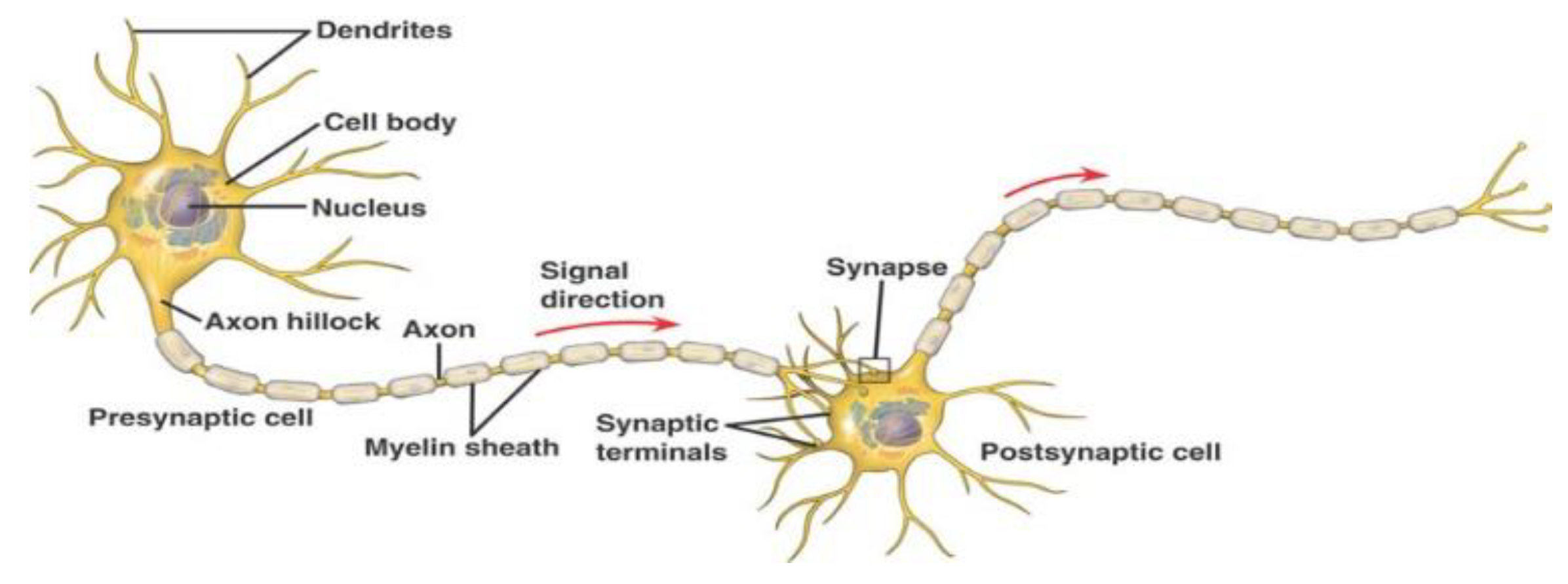
Figure 2.
The NeuCube brain-inspired SNN architecture (from [6]).
Figure 2.
The NeuCube brain-inspired SNN architecture (from [6]).
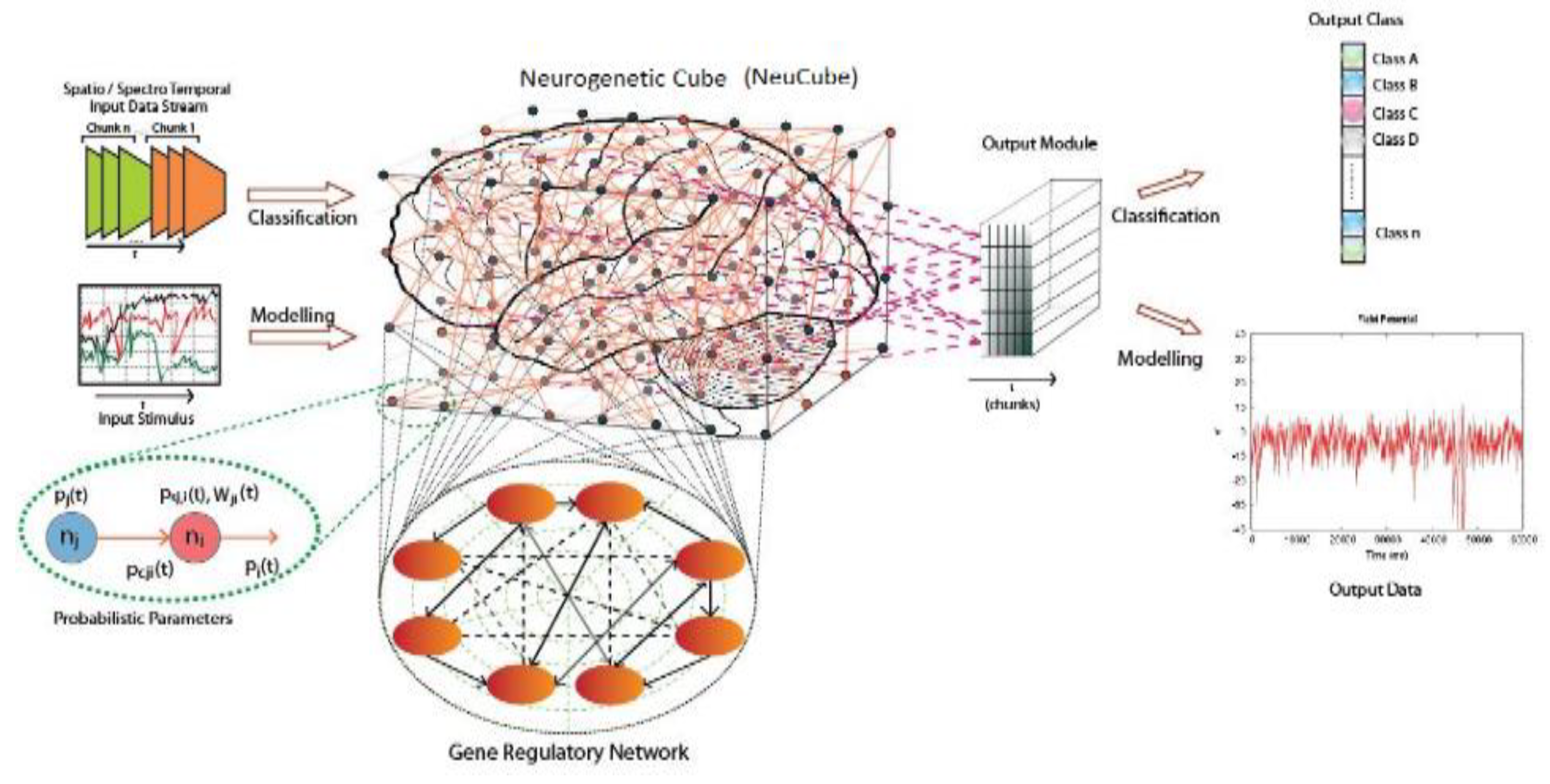
Figure 3.
a. Training NeuCube STAM-EEG model on full data (60 EEG samples). b. Post-training neuronal connectivity and cluster formations. c. Visual depiction of NeuCube's inhibitory and excitatory connections subsequent to training with the Wrist Movement dataset. d. Visual representation of the neuronal spiking activity in NeuCube following the training for the Wrist Movement dataset. e.f. The proportion of input neurons in NeuCube significantly impacts the classification of EEG data associated with wrist movements. (e) EEG electrodes layout (f) NeuCube input neuron proportions in classification results.
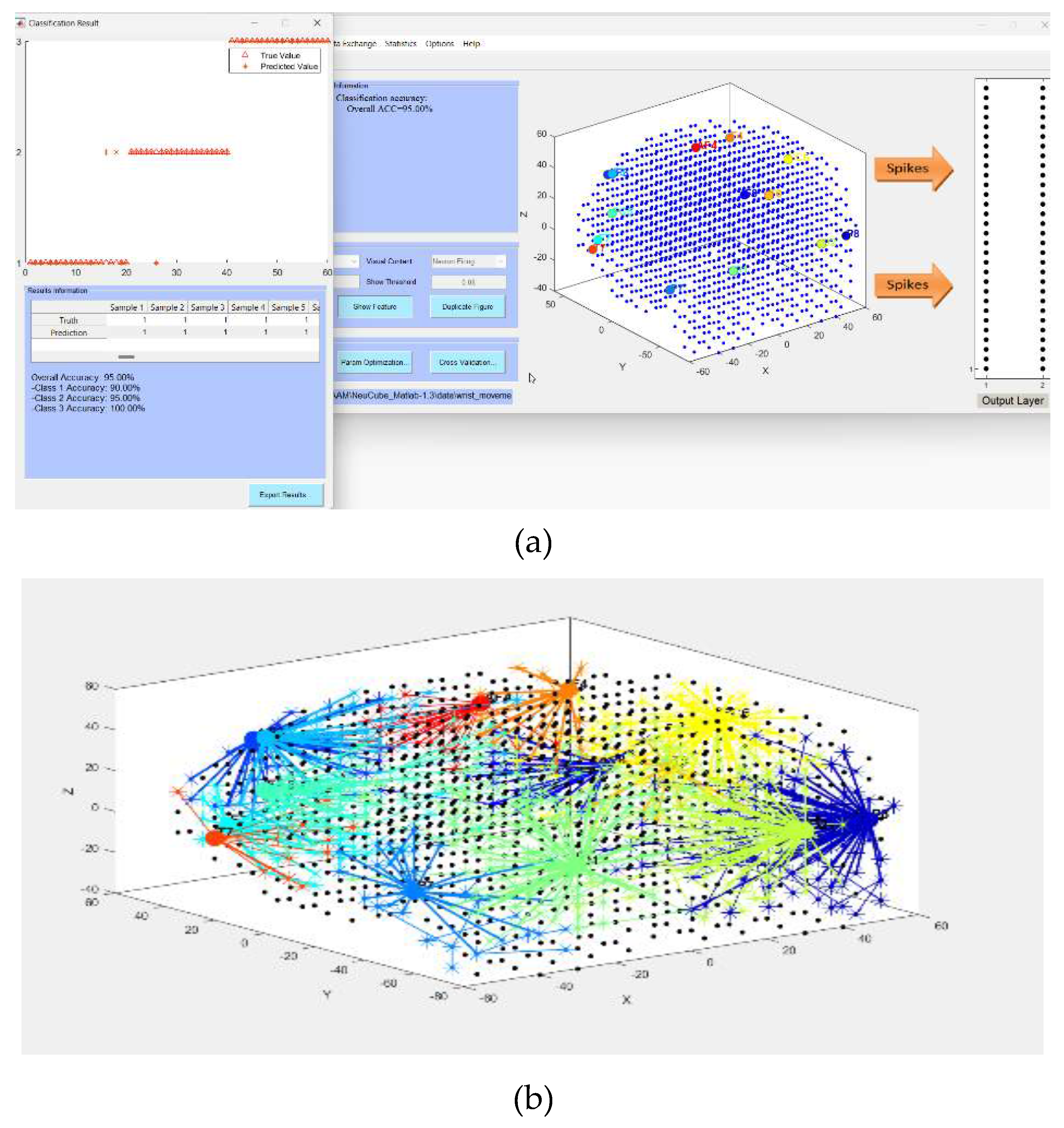
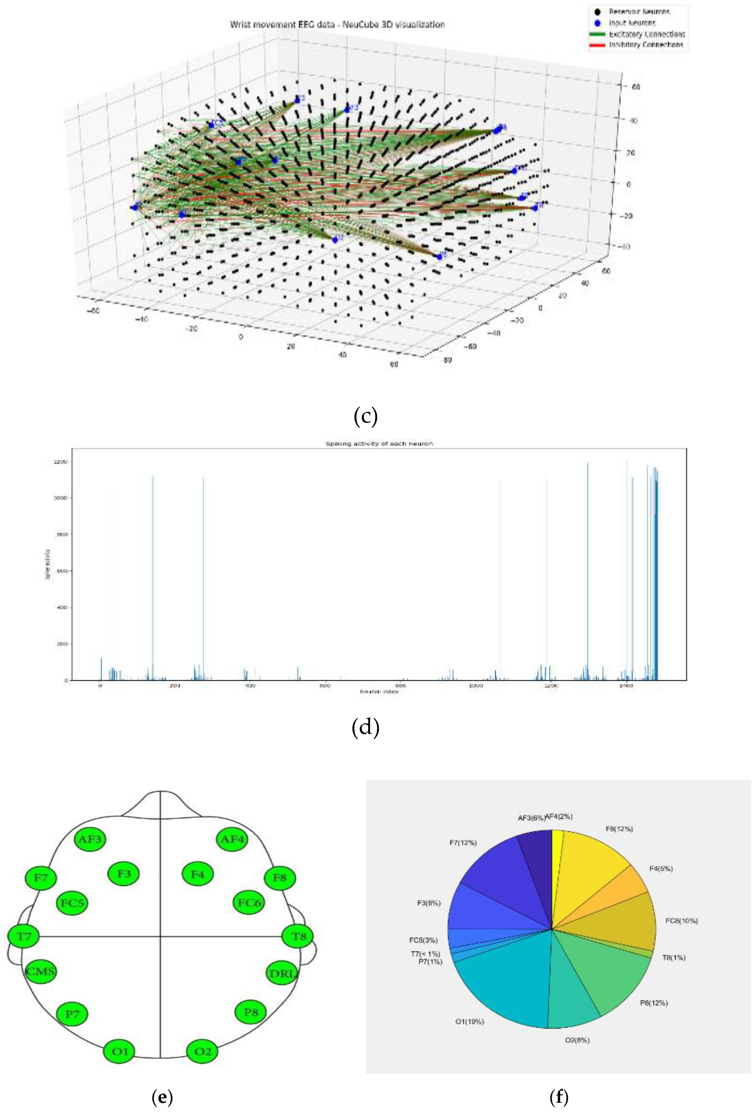
Figure 4.
(a) Mapping of the 5,062 fMRI voxels into a 3D SNN model; (b) selecting the top-20 voxels as input variables using SNR ranking (on the y-axis) of top voxels (on the x-axis) related to the affirmative versus negative sentences. The top voxels were selected according to their SNR values that were greater than a threshold= 0.4. (c) NeuCube model trained and tested on the whole fMRI data time points using all the 40 samples resulted in 100% association accuracy.
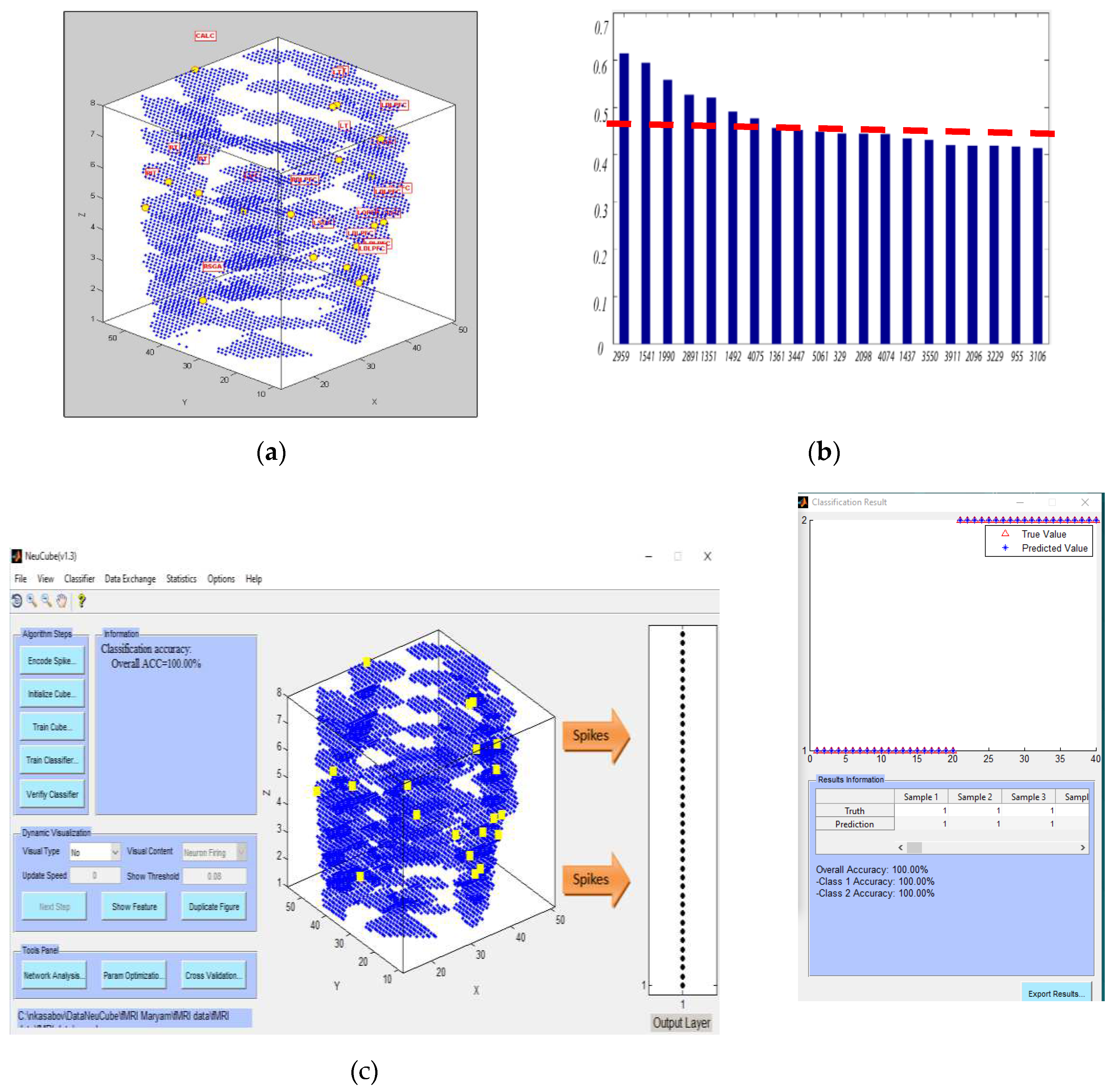
Figure 5.
Three snapshots of learning of 8-second fMRI data in a NeuCube model when a subject is reading a negative sentence (time in seconds); (b) Internal structural pattern represented as spatio-temporal connectivity in the SNN model trained with 8-second fMRI data stream; (c) A functional pattern represented as a sequence of spiking activity of clusters of spiking neurons in a trained NeuCube model.
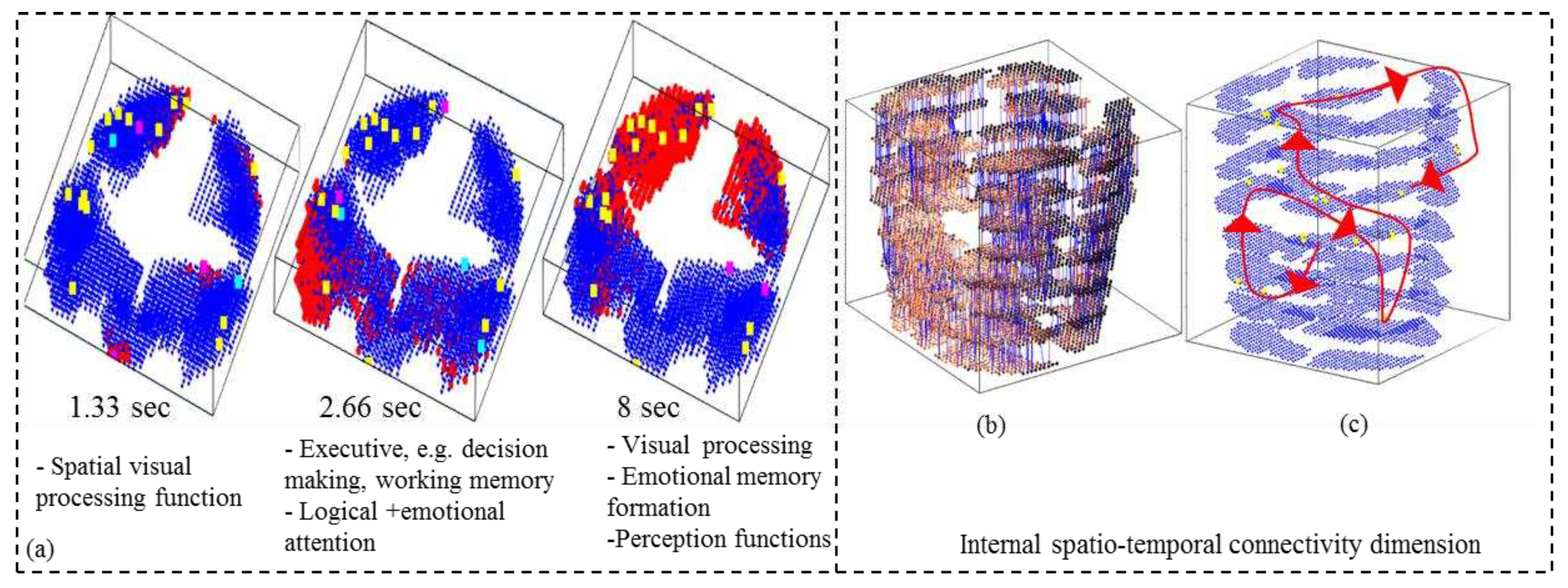
Figure 6.
(a). Left panel: SNNcube was trained using all 40 samples of fMRI data, each had 20 voxels recorded for 8 seconds. However, the trained model was tested by recalling the same 40 fMRI samples, but with a smaller temporal length 70% from the initial timepoint of the fMRI samples equals to 5.6-second data. The classification temporal association accuracy is still 100% as shown in middle panel; and the right pane shows the encoding and testing parameter setting. (b): Left panel: Training the SNNcube with all 40 samples of 16-second fMRI data (20 voxels), while tested by recalling the same 40 fMRI samples with 60% of the temporal length (4.8 second data from 20 voxels). The classification temporal association accuracy is 100% as shown in the middle panel. (c): Training the SNNcube with all 40 samples of 16-second fMRI data (20 voxels), while tested by recalling the same 40 fMRI samples with 50% of the temporal length (4 second data from 20 voxels). The classification temporal association accuracy is 100% as shown in the middle panel. Using less than 50% of the time series results in an accuracy less than 100%.
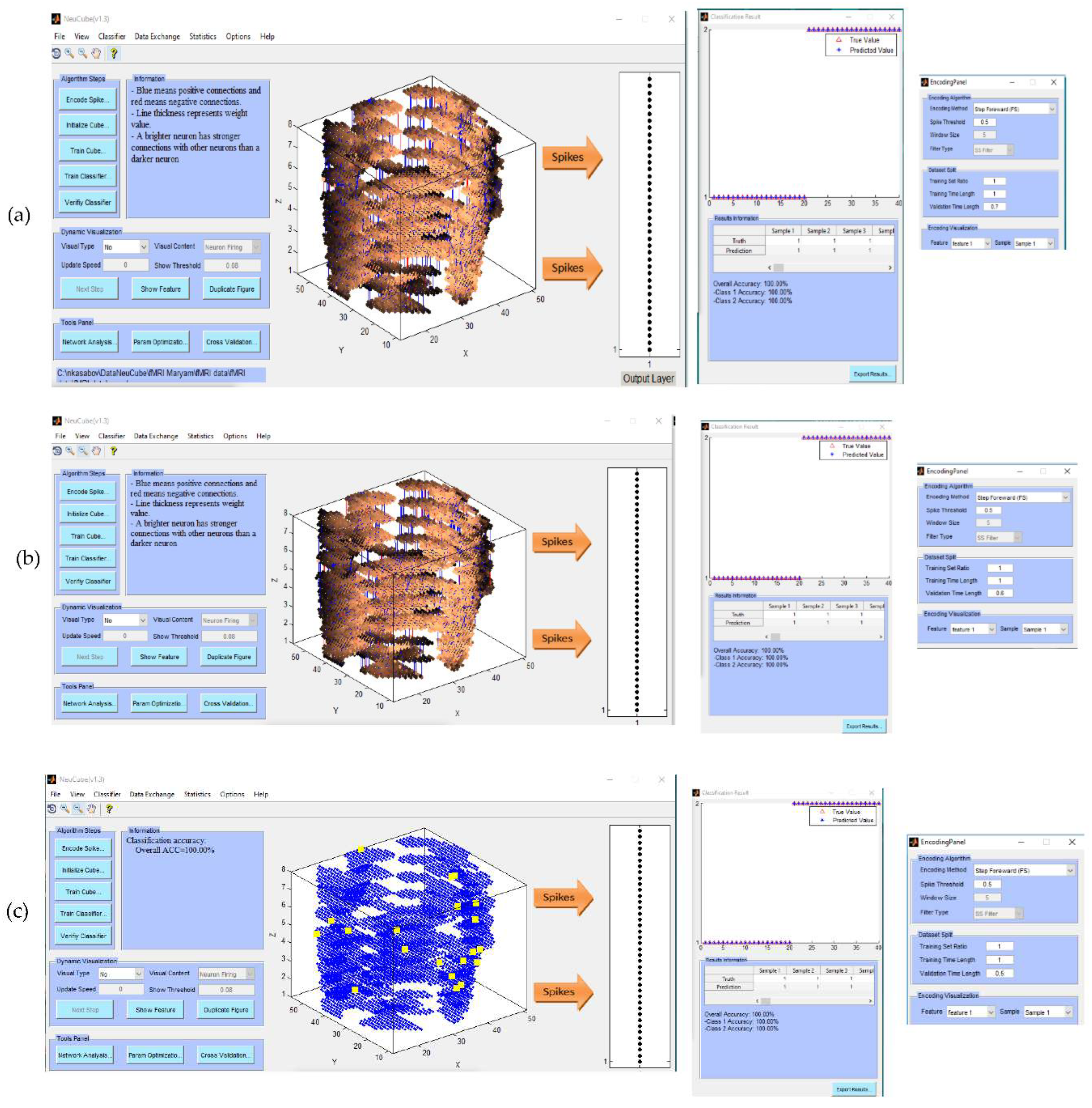
Figure 7.
(a). Left panel: SNNcube was trained using all 40 samples of fMRI data, each had 20 voxels recorded for 8 seconds. However, the trained model was tested by recalling the same 40 fMRI samples, but with a smaller temporal length 70% from the initial timepoint of the fMRI samples equals to 5.6-second data. The classification temporal association accuracy is still 100% as shown in middle panel; and the right pane shows the encoding and testing parameter setting. (b): Left panel: Training the SNNcube with all 40 samples of 16-second fMRI data (20 voxels), while tested by recalling the same 40 fMRI samples with 60% of the temporal length (4.8 second data from 20 voxels). The classification temporal association accuracy is 100% as shown in the middle panel. (c): Training the SNNcube with all 40 samples of 16-second fMRI data (20 voxels), while tested by recalling the same 40 fMRI samples with 50% of the temporal length (4 second data from 20 voxels). The classification temporal association accuracy is 100% as shown in the middle panel. Using less than 50% of the time series results in an accuracy less than 100%.
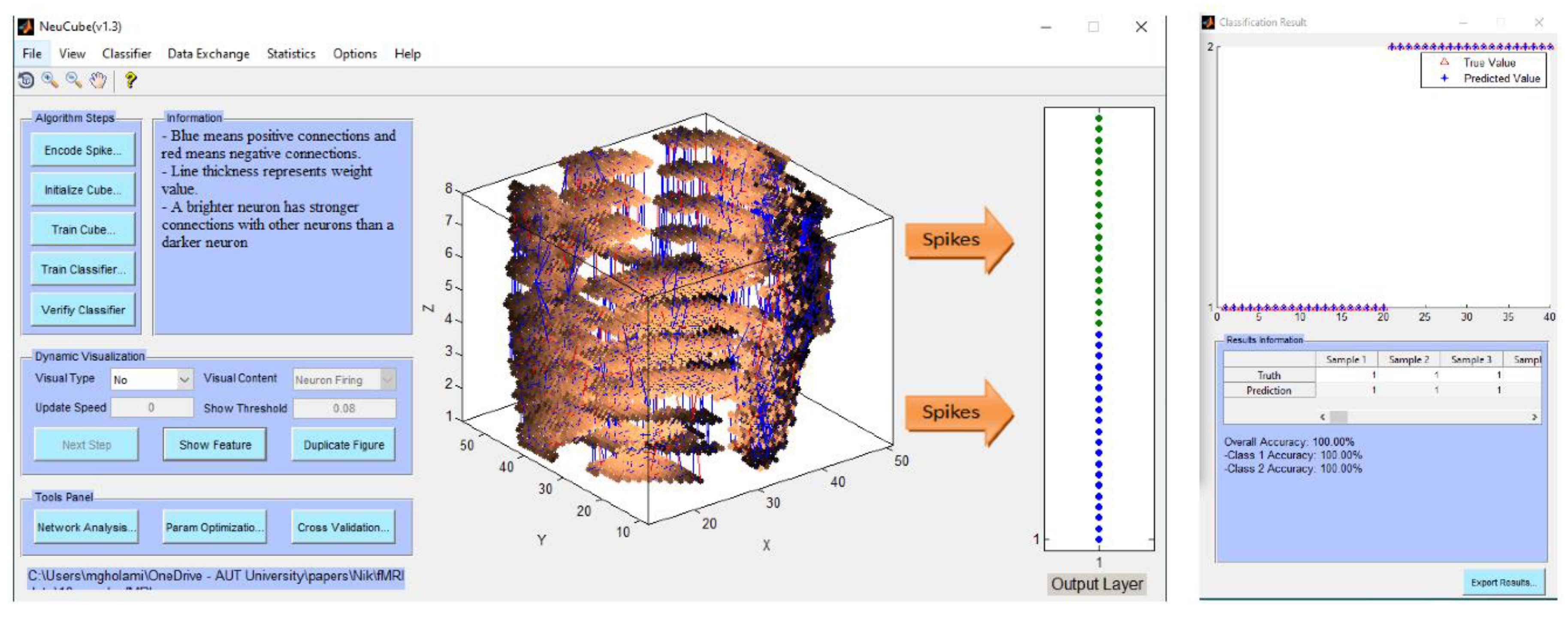
Figure 8.
Distribution of the average connection weights around the input voxels located in the left and right hemispheres of the trained SNN models related to negative sentences (in a) and affirmative sentences (in b). The dominated voxels for the discrimination of the negative and affirmative sentences are: LDLPFC, LIPL, LT and LSGA. .
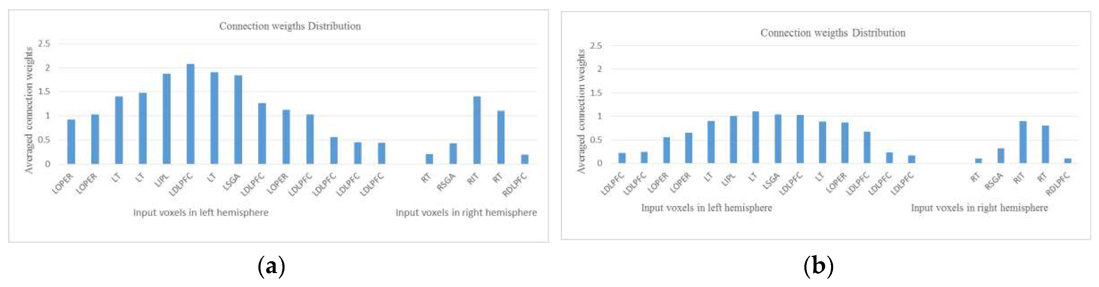

Table 1.
NeuCube STAM-EEG Parameter Settings.
| Dataset information | Encoding method and parameters | NeuCube model | STDP parameters |
deSNNs Classifier parameters |
|---|---|---|---|---|
| sample number: 60, feature number: 14 channels, time length: 128, class number: 3. |
encoding method: Thresholding Representation (TR), spike threshold: 0.5, window size: 5, filter type: SS. |
number of neurons: 1471, brain template: Talairach, neuron model: LIF. |
potential leak rate: 0.002, STDP rate: 0.01, firing threshold: 0.5, training iteration: 1, refractory time: 6, LDC probability: 0. | mod: 0.8, drift: 0.005, K: 3, sigma: 1. |
Table 2.
Classification association accuracy of the NeuCube STAM-EEG model from Figure 3a-e.
Table 2.
Classification association accuracy of the NeuCube STAM-EEG model from Figure 3a-e.
 |
Disclaimer/Publisher’s Note: The statements, opinions and data contained in all publications are solely those of the individual author(s) and contributor(s) and not of MDPI and/or the editor(s). MDPI and/or the editor(s) disclaim responsibility for any injury to people or property resulting from any ideas, methods, instructions or products referred to in the content. |
© 2023 by the authors. Licensee MDPI, Basel, Switzerland. This article is an open access article distributed under the terms and conditions of the Creative Commons Attribution (CC BY) license (http://creativecommons.org/licenses/by/4.0/).
Copyright: This open access article is published under a Creative Commons CC BY 4.0 license, which permit the free download, distribution, and reuse, provided that the author and preprint are cited in any reuse.


