Submitted:
01 August 2023
Posted:
03 August 2023
You are already at the latest version
Abstract
With growing global concern of food and water insecurity, an efficient method to monitor irrigation projects is essential, especially in the developing world, where irrigation performance is often suboptimal. In Nepal, the irrigated area has not been objectively recorded, although their assessment has substantial implications on national policy, project’s annual budgets, and donor fund-ing. Here we present the application of Landsat images to measure irrigated areas in Nepal for the past 17 years to contribute to the assessment of the irrigation performance. Landsat 5 TM (2006-2011) and Landsat 8 OLI (2013-2022) images were used to develop a machine-learning model which classifies irrigated and non-irrigated areas in study areas. The random forest classification achieved overall accuracy of 82.2% and kappa statistics of 0.72. For the class of irrigation areas, the producer’s accuracy and the consumer’s accuracy were 79% and 96%, respectively. Our regionally trained machine-learning model outperforms the existing global cropland map, highlighting the need of such models for local irrigation project evaluations. We assess irrigation project performance and its drivers by combining long-term changes in satellite-derived irrigated area with local data related to irrigation performance, such as annual budget, irrigation service fee, crop yield, precipitation, and main canal discharge.
Keywords:
Landsat
; random forest classification
; performance assessment
; irrigation
; cropland map
; remote sensing
; satellite image
1. Introduction
With the rapid increase in population and growing threats of climate change, there is a global concern for food security [1,2,3,4] and water security [2]. It emphasizes the importance of proper irrigation facilities, reliable cropland maps, and agricultural intensification, particularly in developing countries whose economy is dependent on agriculture. Thus, the improvement of the performance of existing irrigation projects has become important. To improve the performance of irrigation projects, cost-efficient and objective assessments of the performance of irrigation projects are necessary.
Data of irrigated areas have various applications in diverse fields such as water resources management [5], assessment of climate change impacts on irrigation [6], and modeling water exchange in a coupled atmosphere and land surface models [7]. However, in developing countries, like Nepal, the irrigated area has been recorded non-scientifically, relying on visual inspection and local information from local people. However, the recorded irrigated area has substantial implications on donor funding, national policy, annual budgets of projects, and the other relevant decision-making processes.
To improve the capability of monitoring the irrigated area in developing countries, remote sensing serves as a promising tool because of its ability to monitor land surface conditions in a cost-effective way [8] with high accuracy [3,9]. Potapov [3] conducted a global analysis of cropland area changes from 2000 to 2019 using Landsat ARD (Analysis Ready Data). However, the applicability of such globally trained cropland maps for a local or regional irrigation performance assessment was unclear. At local and regional scales, many works classified satellite-derived images to calculate the irrigated area using Landsat [1,9], MODIS [10], and Harmonized Landsat 8 and Sentinel-2 Time Series [11]. However, in these studies, they either took the satellite image of a particular period or used only a single sensor to perform the time series evaluation before the classification, so that their study periods were not long enough to investigate the long-term changes in irrigation performance. Moreover, they focused only on the computation of the irrigated area without any complex quantitative analysis governing the performance of the irrigation system.
It is beneficial to evaluate the performance of irrigation projects and its drivers by integrating satellite-based irrigation maps and the other local data. Both remotely sensed irrigation performance indicators, such as relative evapotranspiration, delivery performance ratio, and drainage ratio, and socio-economic indicators, such as grain yield, price ratio, and water productivity, were used to assess the performance of the irrigation projects [12]. Kumar [13] combined the remote sensing-based estimates of crop production with the water release data from the project and climatic data. Similarly, Higginbottom et al. (2021) examined the relationship between irrigation scheme performance and explanatory variables, the underlying drivers, with a tendency to overpromise and under-deliver in scheme planning for irrigation schemes of Sub-Saharan Africa. However, a thorough evaluation of an irrigation project’s performance and its drivers have not been carried out by comparing the irrigation performance indicators based on relevant local data with the satellite-derived irrigation area.
In this research, we performed cropland mapping for irrigation projects in Nepal using a locally trained classifier and computed the irrigated area for the last 17 years (2006-2022). We performed Random Forest classification, a machine learning-based classification approach, using images from multiple sensors: Landsat 5 TM and Landsat 8 OLI. We realize a cost-effective approach that combines remote sensing derived irrigated areas with locally available data to assess the performance of the irrigation projects. In addition, we compare the performance of a globally trained cropland classification with locally trained models to assess the effectiveness of the global dataset at the local or regional levels.
2. Study Area
Sunsari Morang Irrigation Project (SMIP) is the largest irrigation project in Nepal, whose command area is 68000 ha. We focused on SMIP to collect training and validation points to develop our cropland classification method. To check the robustness of the methodology, our developed methods were also applied to the Bagmati Irrigation System (BIS), the Nepal's second-largest irrigation project with a command area of 45600 ha. Figure 1 shows the location of these two irrigation projects. During monsoon season, typically known as Kharif season in South Asia, the irrigated areas of SMIP and BIS, recorded by the Department of Water Resources and Irrigation, Nepal, were 66000 ha and 39700 ha respectively for every year since 2010 [14] (p. 73), [15] (p. 55), [16] (p. 62), [17] (p. 64), [18] (p. 67), [19] (p. 65), [20] (p. 71), [21] (p. 81), [22] (p. 79), [23] (p. 83), [24] (p. 87). These irrigated areas are, in fact, recorded non-scientifically by the authorized governmental body.
In both regions, farmers grow a variety of crops throughout the year. Major field crops in these areas are paddy, wheat, maize, sugarcane, and several other vegetable crops. In Nepal, a subsistence-based economy, most farmers use the staple crop, paddy, as their primary production, especially in the Kharif season. Due to the reliability of irrigation service in the Kharif season, supported by the rainfall due to the ongoing monsoon, the farmers of the study areas plant paddy as their principal crop during this season. During the Kharif season, the usual planting dates for paddy vary from June to July, and harvesting dates are from late September to early November.
3. Materials and Methods
3.1. Methodological Framework
In our proposed method, the cropland classification maps from 2006 to 2022 in the study areas were provided using the Random Forest classifier in the Google Earth Engine platform. We focused on classifying irrigated areas for paddy, so that Landsat images for July to October, the growing season of paddy, were collected throughout the study period. Typically, there is an active monsoon during the majority of chosen time; thus, almost all the satellite images retrieved in this study had cloud cover. Cloud masking was performed in every image to make cloud-free composites. Depending upon the quality of the cloud-free image collections, the cloud-free composites were grouped as 2-year epochs in the case of Landsat 8 OLI and 3-year epochs in the case of Landsat 5 TM. The image composites were enhanced by adding NDVI and EVI bands as those spectral indices were highly sensitive to vegetation. Spectral Matching of Landsat 5 TM images with the reference image, obtained by taking the median of Landsat 8 OLI image collections from 2013-14 to 2021-22 periods, was done using NDVI and EVI bands. The median image of those enhanced image composites was used for classification using the Random Forests classifier. Training points were taken from high-resolution Google Earth images and Landsat 8 2021-22 images for three different classes: Agriculture, Forest/Pastures, and Non-Agriculture. Those training points were used to train the classifier. After that, the classified images were smoothed to remove the noises and enhance the image's visual quality. Then, the irrigated area was separated from the non-irrigated area, and the sum of pixels classified as Agriculture class in the smoothed image was designated as the total irrigated area.
The irrigation projects’ performance assessment was done by the cropland classification maps and variables collected from various sources. The delivered irrigated area from the classified satellite imageries was compared with the irrigated area recorded by the authorized governmental body, the Department of Water Resources and Irrigation (DWRI). The discrepancy in those two irrigated areas was analyzed. The overall assessment of the irrigation projects was done by comparing the satellite-derived irrigated area with various variables such as yield, Irrigation Service Fee (ISF), project annual budget, main canal discharge, and amount of precipitation contributing to the command area. Those variables included (1) Socio-economic performance indicators: yield and ISF, and (2) factors that influenced the performance of an irrigation project: project annual budget, main canal discharge, and amount of precipitation. Figure 2 shows the general overview of the proposed method.
3.2. Remote Sensing
3.2.1. Data Used
We used Landsat 5 TM and Landsat 8 OLI Surface Reflectance Level 2, Collection 2, and Tier 1 image collections from July to October for the time series evaluation of the irrigation projects. Those images were downloaded from Earth Engine Data Catalog [25,26] from United States Geological Survey (USGS). Blue, Green, Red, and Near Infrared (NIR) bands were used for the image classification, and a QA_PIXEL band was used for masking the clouds. Landsat 5 TM image collections were used from 2006 to 2011, and Landsat 8 OLI from 2013 to 2022. Due to the unavailability of images in 2012, no analysis was done for that particular year. Through visual interpretation, the training samples were manually selected using high-resolution Google Earth imagery along with the Landsat 8 metrics for the 2021-2022 period [1,3]. The GPS coordinates were collected during the field visit to the project’s command area, which was later used for validation.
3.2.2. Google Earth Engine
We used the Google Earth Engine (GEE) cloud environment for the entire assessment which includes satellite image visualization, classification, and command area computation of this study. GEE is a cloud-based platform that provides the capability to retrieve massive satellite images and perform advanced image processing using machine learning algorithms, enabling scientific analysis and visualization of geospatial datasets [27,28,29].
3.2.3. Image Preprocessing
We used atmospherically corrected surface reflectance derived from the data produced by Landsat 5 TM and Landsat 8 OLI. Such Level-2 Surface Reflectance products already include several pre-processing steps, such as atmospheric correction, which enhances the usability of the data for various applications. However, image mosaicking, cloud masking, and implementation of the scaling factor were necessary before the images were used for further analysis and classification.
Image Mosaicking
To create a cohesive and continuous composite image for the study area, image mosaicking, which involves combining multiple satellite images [30], was conducted. The study area, Sunsari Morang Irrigation Project (SMIP), falls on two Landsat tiles, having a path/row combination of 140/41 and 140/42. That is why the region of interest (ROI) was defined to cover the entire study area, including the mosaicked images. The image mosaicking was implemented in GEE. However, Bagmati Irrigation System (BIS) only falls on one Landsat tile- 141/41. In this case, we defined the region of interest without performing the image mosaicking.
Cloud Masking
The satellite images used in this study were masked for cloud cover before classification and further analysis. Cloud masking aims to separate cloud pixels from the rest of the image, allowing for a more accurate and reliable analysis of the underlying features. Since the study area had monsoon seasons throughout the study period from July to October, most of the images had cloud cover, making it challenging to get cloud-free images that could be used for cropland classification. Thus, the cloud masking algorithm was employed for masking the clouds. A binary mask was created for Bit 0, Bit 1, Bit 2, Bit 3, and Bit 4 of the QA_PIXEL band for both Landsat 5 TM and Landsat 8 OLI. Similarly, a binary mask was also created for the QA_RADSAT band for both satellites.
Scaling Factor
The optical and thermal bands were converted from digital number (DN) to reflectance and brightness temperature, respectively, using the scaling factor in this study prior to further analysis and classification of the image. The data provided for ‘Scale’ and ‘Offset’ for various optical and thermal bands on the Earth Engine Data Catalog for both the satellites: [25] for Landsat 5 TM and [26] for Landsat 8 OLI, were used for this operation.
3.2.4. Image Composites
We took two years of image composites for Landsat 8 OLI and three years for Landsat 5 TM. From several sensitivity analyses, we found two years of cloud-free image composite yielded a complete image throughout the composite periods, a total of five, from 2013 to 2022 for Landsat 8 OLI. However, the three years cloud-free image composite only yielded a reasonable result for Landsat 5 TM for two composite periods from 2006 to 2011. No retrievable image was available for 2012 in Landsat 5 TM, so that this particular year was neglected in our study.
3.2.5. Spectral Indices
We chose spectral indices, NDVI and EVI, which are highly sensitive to vegetation’s presence and vigor. NDVI has been widely used as an indicator for irrigated areas [11,31] since it detects changes in vegetation reflectance, especially for the forest, agriculture, and crop types [10]. Similarly, EVI for cropland mapping [8,31] can provide valuable insights into vegetation conditions, stress levels, and crop health. Thus, NDVI and EVI bands were added to the original bands of the collection of images grouped as cloud-free image composites, and enhanced collection composites were obtained. Then, the median images for each enhanced collection composite were computed and used for classification.
3.2.6. Spectral Matching
Spectral Matching [32,33,34,35] was performed on enhanced image composites of Landsat 5 TM before classification. We obtained unsatisfactory results when we directly applied the same classifier trained with high-resolution Google Earth image and Landsat 8 OLI image to Landsat 5 TM images due to the differences in spectral characteristics between the two satellite sensors.
To address this issue, a two-step approach was taken. Firstly, a reference image was obtained by computing the median of all the enhanced image composites for Landsat 8 OLI. Secondly, the NDVI and EVI bands of the enhanced images of Landsat 5 TM were then subtracted and multiplied from the corresponding NDVI and EVI bands of the reference image. Those NDVI difference and NDVI ratio were applied to the NIR band of Landsat 5 TM enhanced image, producing a matched NDVI band. The same technique was applied to compute the matched EVI band. Adding these matched NDVI and EVI bands to the Landsat 5 TM enhanced image composites, a set of matched image composites suitable for classification was obtained.
The NIR band was explicitly chosen for spectral matching due to its significance in vegetation analysis, as it captures the reflectance of healthy vegetation, which is typically higher in the NIR region. Applying spectral matching to the NIR band aims to ensure consistent and comparable spectral information related to vegetation, including crops, across different images. This process enhances the accuracy and comparability of cropland classification by reducing spectral variations and ensuring consistent representation of vegetation-related features across different images or datasets.
3.2.7. Feature Extraction
The extraction of features for the training dataset was performed, covering the spatial extent of the entire study for the 2021-22 period. The training points were collected for three classes: Agriculture, Non-Agriculture, and Forest/Pastures. The number of training samples used per class was:
- ▪
- Agriculture class- 424
- ▪
- Non-Agriculture class- 898
- ▪
- Forest/Pastures class- 222
3.2.8. Cropland Classification
We performed the cropland classification of the median image using the Random Forest (RF) classifier [1,2,8,36], a supervised classification technique. The RF classifier's accuracy and output were insensitive to variations in the number of trees and the maximum depth of each tree. This feature demonstrates the classifier's robustness against overfitting in various settings. We perfromed the experiments with the various combinations, including 50/50, 75/75, 100/75, 100/100, 200/100, 200/200, 500/100, and 1000/100 for the number of trees and maximum depth. The Overall Accuracy (OA) ranged from 0.809 to 0.8219, Kappa metrics from 0.697 to 0.721, and Out of Bag Error Estimate from 0.126 to 0.136 for these combinations. Notably, when the number of trees was tuned to 200, and the maximum depth of each tree was set to 75, a slightly better result was obtained with an Overall Accuracy (OA) of 82.19%, Kappa Coefficient of 0.721, and Out of Bag Error Estimate of the classifier at 0.1258, compared to different combinations of these parameters. We show the results obtained by this hyperparameter set in this paper.
3.2.9. Smoothing of Classified Image
We performed spatial smoothing (neighborhood mode) which includes erosion and dilation. The circular kernel of radius 1 was slid through the image. During erosion, a pixel in the original image (1 or 0) was considered 1 only if all the pixels under the kernel were 1. Otherwise, it was eroded (made to 0). Through this process, all the pixels near the boundary were discarded, decreasing the foreground object's thickness or size. It helped remove small noises.
Dilation is conceptually opposite to erosion. A pixel element was considered 1 if at least one pixel under the kernel was 1. It increased the size of the foreground object. Totally, two iterations were performed for both the erosion and dilation processes during the smoothing operation.
3.2.10. Delivered Irrigation Area
The irrigated area map was created by separating irrigated and non-irrigated areas from the smoothed image. The Agriculture class of the smoothed image was separated from the other two classes: Non-Agriculture class and Forest/Pastures class. The area covered by the Agriculture class was designated as irrigated area, whereas the other two classes were designated as non-irrigated area. We assumed that all the Agriculture class is associated with irrigation water supply in our study areas. Subsequently, a binary map of the irrigated area was generated for the study period.
3.2.11. Validation
The ground truth samples collected during the field visit from March 6 to March 15, 2023, were used to validate the classification result. GPS coordinates representing all three classes (Agriculture, Non-Agriculture, and Forest/Pastures) were collected during the visit. While collecting the coordinates, we made sure that the ground truth samples include the data from head to tail end of the command area and are representative of both Sunsari and Morang districts to to minimize any biases in the data. The number of the validation samples collected per class was:
- ▪
- Agriculture class- 290
- ▪
- Non-Agriculture class- 139
- ▪
- Forest/Pastures class- 127
3.2.12. Accuracy Assessment
In this study, overall accuracy, producer’s accuracy, consumer’s accuracy, and kappa coefficient were used to assess the accuracy of Random Forest classifier [37,38,39,40,41,42]. The classifier's overall accuracy was assessed by dividing the total count of pixels that were correctly classified by the total count of reference pixels. Consumer's accuracy, for each category was calculated by dividing the number of correctly classified pixels belonging to that category by the total count of pixels in that category's column. On the other hand, producer's accuracy, was determined by dividing the number of correctly classified pixels in each category (found along the major diagonal; see Table 1) by the total count of test set pixels used for that specific category (the row total; see Table 1).
The kappa statistic was computed using the following formula:
where:
r = number of rows in the error matrix
xii = number of observations in row i and column i
xi+ = total number of observations in row i
x+i = total number of observations in column i
N = total number of observations included in matrix
3.3. Performance Assessment of Irrigation Projects
Our performance assessment of irrigation projects includes the evaluation of irrigation performance, its drivers, and the value added by the irrigation systems. ISF was used as the proxy of the irrigation performance, whereas paddy yield represents both the performance indicators and the value for farmers added by the irrigation system. Both the data of ISF collected from the project’s beneficiary farmers [14] (p. 82), [15] (p. 62), [16] (p. 69), [17] (p. 69), [18] (p. 72), [19] (p. 70), [20] (p. 76), [21] (p. 86), [22] (p. 84), [23] (p. 88), [24] (p. 92), and paddy yield (MT/ha) for the Kharif season [14] (p. 86), [15] (p. 67), [16] (p. 74), [17] (p. 74), [18] (p. 76), [19] (p. 74), [20] (p. 80), [21] (p. 90), [22] (p. 88), [23] (p. 92), [24] (p. 96) were obtained from the DWRI, Nepal. National average yield of paddy [43] (p. 5), [44] (p. 11) is also obtained from the Ministry of Africultural Development (MoALD) of Nepal. The variables that impact the project’s performance, which we call drivers, such as amount of precipitation, project’s annual budget [14] (p. 73), [15] (p. 55), [16] (p. 62), [17] (p. 64), [18] (p. 67), [19] (p. 65), [20] (p. 71), [21] (p. 81), [22] (p. 79), [23] (p. 83), [24] (p. 87), and discharge in the main canal, were collected. Monthly (July to October) precipitation data from five rainfall stations that lied within or contributed to the command area runoff were collected from the Department of Hydrology and Meteorology (DHM), Nepal. Discharge of the main canal was obtained from the project office. The monetary variables, i.e. ISF and the project’s annual budget, were converted using Consumer Price Index (CPI), taking the year 2014.15 as the base period according to the guidelines provided by the Nepal Rastra Bank (NRB), the central bank of Nepal [45] (p. 419), [46] (p. 447).
4. Results
4.1. Accuracy Assessment of the Classifier
Table 1 shows the confusion matrix obtained from the classified map 2021-22 to evaluate the performance of our classifier. The overall accuracy and kappa coefficient were 82.2% and 0.72, respectively. The producer’s and consumer’s accuracy for the Agriculture class, the class used to separate the irrigated area in this study, was 79% and 96%, respectively. Non-Agriculture class had consistently better accuracies, with both producer’s and consumer’s accuracy above 80%; however, there was greater variability in the Forest/Pastures class. This class had an excellent producer’s accuracy of 90%, whereas the consumer’s accuracy is insufficient (63%). In fact, the 53 samples of the Agriculture class were misclassified, thus resulting in a lower producer’s accuracy for the Agriculture class (79%) and lower consumer’s accuracy for the Forest/Pastures class (63%). From the spectral signature shown in Figure 3, the spectral characteristics of the Agriculture class and Forest/Pastures class were similar although the Agriculture class has a slightly higher reflectance value in the NIR region. This is why the samples of the Agriculture class were usually misclassified as the Forest/Pastures class.
4.2. Cropland Classification
The cropland classification maps were obtained for the study areas by separating the irrigated areas from non-irrigated ones. Figure 4 shows the cropland classification maps of SMIP from 2006 to 2022, where the classified image obtained from Landsat 5 TM was represented in a three-year epoch, i.e., 2006-08 and 2009-11, and for the one obtained from Landsat 8 OLI, in a two-year epoch- 2013-14, 2015-16, 2017-18, 2019-20 and 2021-22. There are two important implications in Figure 4. First, the tail-end portion, the southern part of the command area, was not fully irrigated although some improvements can be found in the later years (2017-18 and 2021-2022 periods). The tail-end portions of the command area lack irrigation facilities necessary for surface irrigation. However, the gradual increment in 2017-18 and 2021-22 shown in Figure 4 implies that the irrigation system was adequately managed and there was proper water management. Second, the irrigated area in the 2019-20 period was significantly declined especially in the eastern part of the command area of the project. This is because the major flood occurred in 2017 [47], which damaged the aqueduct of the main canal, which deprives the irrigation facility in that part of the command area.
Figure 5 shows the cropland classification maps of BIS from 2013 to 2022. Due to the unavailability of good-quality images obtained from Landsat 5 TM for the command area during the study period 2006 to 2012, the satellite images obtained from Landsat 8 OLI were only used. We found that the area under agriculture significantly increased in 2017-18, 2019-20, and 2021-22 compared to the initial years.
4.3. Recorded vs Satellite Derived Irrigated Area
Figure 6 compares the satellite-derived irrigated area and the irrigated area recorded by the DWRI for both SMIP and BIS throughout the study period. The irrigated area of the irrigation projects obtained from our cropland classification maps substantially changes over time. However, DWRI reported the constant values of irrigated area which are 66000 ha for SMIP and 39700 ha for BIS during the Kharif season. In the case of SMIP, the satellite-derived irrigated area was less than the area recorded by the DWRI by at least 8000 ha every year. As we discussed, the total irrigated area increased from 2006 to 2018 and suddenly declined in the 2019-2020 period due to the effect of flooding. The dynamics of the irrigated area was not recorded by the DWRI. For BIS, the irrigated area consistently improved over the years, surpassing the DWRI’s recorded values for the 2017-18 and 2021-22 periods. It indicates a significant achievement by BIS in expanding the irrigated area, which has been overlooked by DWRI.
4.4. Comparison of Classification Result with Globally Trained Cropland Classification
Our cropland classification map trained by the local dataset is substantially different from the globally trained cropland classification map provided by [3]. When the Global Cropland Classification Map (GCCM) provided by [3] was compared with our estimated cropped area, as shown in Figure 7, GCCM classifies most of the command area as stable cropland, which is inconsistent to our findings. Regarding the tail-end portions of the command area, the globally trained cropland classification map has overestimated the cropland area throughout the study period, as shown in Figure 7a–f. Most importantly, the global cropland map only showed a minor change in the cropland area throughout the study period, and it does not replicate the cropland area loss caused by a major flood event in 2019-20, as shown in Figure 7f. These results indicate that an existing global cropland map cannot accurately reproduce the small-scale distribution of irrigated land.
4.5. Performance Assessment of the Project
4.5.1. Performance Indicators
Socioeconomic indicators were used to assess the performance of the projects. For that purpose, paddy yield and ISF of the command area were compared with the irrigation area discussed above.
Yield
Figure 8 shows the timeseries of paddy yield, measured in Metric Ton per Hectare (MT/ha) with the change in irrigated area. As far as SMIP is concerned, the annual yield of paddy was meager in the year 2009-10; however, with the increase in irrigated area, there was almost a linear increase till 2019.20. The SMIP irrigation project successfully increased not only irrigated area, but also the production performance per area. For BIS, the yield remained relatively constant until 2019.20, although in the last two years, 2020.21 and 2021.22, there was an increase in yield, accompanied by an increase in the irrigated area. As the cropped area expanded, there was a tendency for higher yields.
The provision of irrigation facilities substantially improved the paddy yield compared to the ones that did not get those facilities, thus, justifying the value added by those irrigation projects. Figure 9 compares the projects’ annual paddy yield (MT/ha) with the national average. There was an increase in paddy yield over time, with an almost linear trend observed across all three sectors: SMIP, BIS, and national average. Both irrigation projects consistently showed higher yields than the nationwide averaged yield, with only one exception for SMIP in 2009-10 when the yield was less by 0.255 MT/ha compared to the national average. In the case of BIS, this difference with the national average reached as high as 2.246 MT/ha during 2015/16.
Irrigation Service Fee Collection
The amount of ISF collected from the beneficiary farmers depends on the reliability of the irrigation service provided by the project office. Although there is a provision in the national policy to collect ISF, it has not been effectively carried out. The farmers provide the fee only if they are satisfied with the system. Thus, the ISF can be viewed as a measure of farmers' satisfaction with the reliability of irrigation system performance. Fluctuations in the collection of ISF can be seen in both the irrigation projects, SMIP and BIS, as shown in Figure 10. In the case of SMIP, there was a significant fluctuation in ISF throughout the study period, with the least ISF collected in 2011.12. After 2012, the ISF collection improved almost linearly till reaching the peak in 2016.17, accompanied by the project office's delivery of constantly increased irrigated areas. This was followed by a sharp drop till 2019.20 due to decreased irrigated area. With an increase in the irrigated area in 2021.22, there was a significant improvement in ISF collection. In the case of BIS, although there was an almost linear increase in the irrigated area throughout the study period, the ISF collection displayed a different trend. There was an increase in the second year of collection compared to the first year (2015.16), which remained relatively constant the following year. Then there was a steep drop in 2018.19, followed by a linearly increasing trend. One of the reasons behind this could be the reduction in the annual budget allocated to BIS for 2019.20 (refer to Figure 11). Generally, in Nepal, the ISF of a particular year is collected at the end of that fiscal year. In contrast, the annual budget for the upcoming year is allocated at the end of the previous fiscal year. Therefore, the annual budget of BIS for 2019.20 was allocated at the end of 2018.19, and a sharp decline in this value may have impacted the farmer's reluctance to give the ISF, thus reducing the ISF collection for 2018.19.
4.5.2. Variables Impacting Project performance
Project Annual Budget
The operation and maintenance of large irrigation projects like SMIP and BIS required a substantial amount of annual budgets, and variations on those funds had a significant impact on the performance of the projects. Figure 11 shows the timeseries of the annual budgets as well as the estimated irrigated area in SMIP and BIS. An increasing trend in the allocation of annual budgets for SMIP can be observed from 2006.07 to 2016.17, while for BIS, a similar trend was seen only from 2013.14 to 2014.15, and then it was almost constant till 2018.19. An increase in the irrigated area accompanied those periods of increased or constant budget allocation. Conversely, a decline in the budget can be observed for SMIP from 2016.17 to 2019.20, and for BIS, from 2018.19 to 2019.20, which corresponded to a decrease in the irrigated area.
Furthermore, after 2019.20, an increase in the budget was followed by a corresponding increase in the irrigated area for both projects. In particular, in SMIP, the annual budget allocated for 2021.22 is as twice as the amount allocated in 2020.21. This increased budget was primarily directed toward repairing the canals damaged by floods, with a specific focus on constructing the damaged aqueduct.
Discharge of Main Canal
The fluctuations in the discharge diverted to the main canal had a minimal impact on the irrigated area of the project, as shown in Figure 12. Although the discharge in the main canal of SMIP was fluctuating, the irrigated area remained relatively constant throughout the study period, except for a decrease in the irrigated area for the years 2019.20 and 2020.21 due to the damage caused by flood, as explained in section 4.2. Despite the variations in the main canal discharge, water management plans were implemented correctly, and the project effectively managed the irrigation system.
Amount of Precipitation
The data of precipitation amounts were collected from the rainfall stations within the command area or the ones which had the runoff contribution to the command area of SMIP. Figure 13 shows how the variation of rainfall amount in the rainfall stations was related to the irrigated area. From 2006.07 to 2010.11, an increase in rainfall within the command area also led to an increase in the irrigated area. Despite a decreasing trend in rainfall from 2010.11 till 2018.19, the irrigated area remained almost constant, indicating effective water management and overall system management. However, a significant increase in rainfall occurred in 2019.20 and 2020.21, causing floods and damaging the irrigation system, which resulted in a substantial drop in the irrigated area.
5. Discussion
Classifiers for cropland detection were trained and validated using training data collected from visual interpretation of Landsat and Google Earth images by [1,3,9]. In this study, we utilized training data from Landsat 8 OLI 2021-22 and Google Earth image, validated using ground truth points, thus offering local relevance and accurate results. The producer’s accuracy we obtained in this classification for the Agriculture class of 79% was comparable with [1] for the irrigated class, which was 80%. Our obtained accuracy is also comparable with the global study [3], which ranged from 70.3% to 86.4% for cropland.
The method we employed in this study provides a real-world representation of spatial patterns of irrigated areas, allows scalability, and reduces cost compared to the use of ground truth points alone, as done by [11]. However, the overall accuracy and Kappa statistics of [11], which are 90.6% and 0.82, respectively, were higher than our method. Note that we trained our classifier by visual interpretation of images and validated it by ground truth data, so that our training and validation data come from different sources. This problem setting may be more difficult to obtain good accuracies than [11], in which both training, and validation data came from ground truth points.
In Sub-Saharan Africa, over-optimistic planning as a response to political pressure results in poor projections, over-promising benefits, and underestimating costs [1]. Similarly, in Nepal, the same reason has caused overestimation and underdelivering as far as the official record of the irrigated area is concerned in the case of SMIP. Regarding irrigation system management, SMIP demonstrates the strong performance in its ability to recover swiftly from significant flooding events that caused a decline in the irrigated area during the 2019.20 and 2020.21 periods. BIS exhibits consistent improvement in performance, specifically regarding the expansion of the irrigated area, throughout the study period. These observations highlight the favorable performance of both SMIP and BIS compared to Sub-Saharan African irrigation projects shown in [1].
The globally trained cropland classification map [3] substantially overestimates cropland areas and is inconsistent to our locally trained cropland maps. Therefore, for accurate local or regional performance assessments of cropland classification, relying solely on globally trained results is not advisable.
Only one growing season is considered in this study, as done by [9,11,12,13]. Paddy, as used by [12,13], the staple food crop in developing countries, is used for the analysis in this study for one growing season. While we have focused on mapping the irrigated areas for paddy at a local level, a similar methodology of cropland mapping can be done on regional and local scales for diverse crop types, extending beyond the scope of the current study. Also, it would be intriguing to conduct a comparison between the classification outcomes achieved in this study and those obtained through the implementation of alternative methodologies such as transfer learning, which considers the spatial diversity of class distributions [48], and deep learning approaches, which can effectively handle substantial training datasets [49]. Complex quantitative analysis of various climatic and economic factors (other than the ones discussed in this study) and socio-political factors governing scheme performance is promising for future works.
6. Conclusions
In this study, we analyzed the change in the cropped area of irrigation projects: Sunsari Morang Irrigation Project (SMIP) and Bagmati Irrigation System (BIS) of Nepal from 2006 to 2022 using locally calibrated cropland classification maps. By comparing the satellite-derived irrigated areas with the ones recorded in the government data books, it was found that they overestimated the irrigated area for SMIP throughout the entire study period. In contrast, the satellite-derived irrigated area exceeded the data records for 2017-18 and 2021-22 in the case of BIS.
The Random Forest classifier used for cropland classification was trained using the training points obtained from visual interpretation of Google Earth and Landsat 8 OLI 2021-22 image. The classification result was validated using the ground truth points from the project site. The accuracy assessment showed an overall accuracy of 82.2% and a Kappa coefficient of 0.72, with producer’s and consumer’s accuracy for the Agriculture class, the class used to separate irrigated from the unirrigated area, was 79% and 96%, respectively. The variables required for the performance assessment were collected from various local sources, then compared with the irrigated area throughout the study period. The thorough assessment of the performance of the irrigation project was done in a cost-effective and timely manner. This method can be employed by the DWRI, Nepal, as an assessment method for other irrigation projects throughout the country.
By comparing the locally calibrated cropland map obtained from this study with the global cropland classification map for the study area, we discovered that only locally trained maps could accurately replicate the precise allocation of irrigated land at a small scale. Therefore, these maps are necessary for conducting performance assessments of irrigation projects at the local level.
Supplementary Materials
The following supporting information can be downloaded at the website of this paper posted on Preprints.org, Code: Cropland Classification using Landsat 8 and Landsat 5 metrics.
Author Contributions
Conceptualization, A.N. and Y.S.; methodology, A.N.; software, A.N.; formal analysis, A.N. and Y.S.; investigation, A.N.; resources, Y.S.; data curation, A.N.; writing—original draft preparation, A.N.; writing—review and editing, A.N. and Y.S.; visualization, A.N.; supervision, Y.S.; project administration, A.N.; funding acquisition, Y.S. All authors have read and agreed to the published version of the manuscript.
Funding
This study was supported by the KAKENHI grant 21H01430.
Acknowledgments
We acknowledge the SMIP project team for providing project specific data, and DHM, Nepal for providing the precipitation data.
Conflicts of Interest
The authors declare no conflict of interest.
References
- Higginbottom, T.P.; Adhikari, R.; Dimova, R.; Redicker, S.; Foster, T. Performance of Large-Scale Irrigation Projects in Sub-Saharan Africa. Nat. Sustain. 2021, 4, 501–508. [Google Scholar] [CrossRef]
- Magidi, J.; Nhamo, L.; Mpandeli, S.; Mabhaudhi, T. Application of the Random Forest Classifier to Map Irrigated Areas Using Google Earth Engine. Remote Sens. 2021, 13, 876. [Google Scholar] [CrossRef]
- Potapov, P.; Turubanova, S.; Hansen, M.C.; Tyukavina, A.; Zalles, V.; Khan, A.; Song, X.-P.; Pickens, A.; Shen, Q.; Cortez, J. Global Maps of Cropland Extent and Change Show Accelerated Cropland Expansion in the Twenty-First Century. Nat. Food 2022, 3, 19–28. [Google Scholar] [CrossRef] [PubMed]
- Tariq, A.; Yan, J.; Gagnon, A.S.; Riaz Khan, M.; Mumtaz, F. Mapping of Cropland, Cropping Patterns and Crop Types by Combining Optical Remote Sensing Images with Decision Tree Classifier and Random Forest. Geo-Spat. Inf. Sci. 2022, 0, 1–19. [Google Scholar] [CrossRef]
- Vörösmarty, C. Global Water Assessment and Potential Contributions from Earth Systems Science. Aquat. Sci. 2002, 64, 328–351. [Google Scholar] [CrossRef]
- ALCAMO, J.; DÖLL, P.; HENRICHS, T.; KASPAR, F.; LEHNER, B.; RÖSCH, T.; SIEBERT, S. Global Estimates of Water Withdrawals and Availability under Current and Future “Business-as-Usual” Conditions. Hydrol. Sci. J. 2003, 48, 339–348. [Google Scholar] [CrossRef]
- Boucher, O.; Myhre, G.; Myhre, A. Direct Human Influence of Irrigation on Atmospheric Water Vapour and Climate. Clim. Dyn. 2004, 22, 597–603. [Google Scholar] [CrossRef]
- Bendini, H.; Sanches, I.; Körting, T.; Fonseca, L.; Luiz, A.; Formaggio, A. USING LANDSAT 8 IMAGE TIME SERIES FOR CROP MAPPING IN A REGION OF CERRADO, BRAZIL. ISPRS - Int. Arch. Photogramm. Remote Sens. Spat. Inf. Sci. 2016, XLI-B8, 845–850. [Google Scholar] [CrossRef]
- Traoré, F.; Bonkoungou, J.; Compaoré, J.; Kouadio, L.; Wellens, J.; Hallot, E.; Tychon, B. Using Multi-Temporal Landsat Images and Support Vector Machine to Assess the Changes in Agricultural Irrigated Areas in the Mogtedo Region, Burkina Faso. Remote Sens. 2019, 11, 1442. [Google Scholar] [CrossRef]
- Ambika, A.K.; Wardlow, B.; Mishra, V. Remotely Sensed High Resolution Irrigated Area Mapping in India for 2000 to 2015. Sci. Data 2016, 3, 160118. [Google Scholar] [CrossRef] [PubMed]
- Falanga Bolognesi, S.; Pasolli, E.; Belfiore, O.R.; De Michele, C.; D’Urso, G. Harmonized Landsat 8 and Sentinel-2 Time Series Data to Detect Irrigated Areas: An Application in Southern Italy. Remote Sens. 2020, 12, 1275. [Google Scholar] [CrossRef]
- Bandara, K.M.P.S. Assessing Irrigation Performance by Using Remote Sensing; ITC dissertation; ITC: Enschede, 2006; ISBN 978-90-8504-406-2. [Google Scholar]
- Kumar K, A. Irrigation Performance Assessment of Left Bank Canal, Nagarjuna Sagar Project, India During Rabi Using Remote Sensing and GIS. Agrotechnology 2014, 03. [Google Scholar] [CrossRef]
- IrrigationYearBook2010.11. Available online: https://www.dwri.gov.np/files/notice/20210804064529.pdf (accessed on 20 June 2023).
- IrrigationYearBook2011.12. Available online: https://www.dwri.gov.np/files/notice/20210804064529.pdf (accessed on 20 June 2023).
- IrrigationYearBook2012.13. Available online: https://www.dwri.gov.np/files/notice/20210804064529.pdf (accessed on 20 June 2023).
- IrrigationYearBook2013.14. Available online: https://www.dwri.gov.np/files/notice/20210804064529.pdf (accessed on 20 June 2023).
- IrrigationYearBook2014.15. Available online: https://www.dwri.gov.np/files/notice/20210804064529.pdf (accessed on 20 June 2023).
- IrrigationYearBook2015.16. Available online: https://www.dwri.gov.np/files/notice/20210804064529.pdf (accessed on 20 June 2023).
- IrrigationYearBook2016.17. Available online: https://www.dwri.gov.np/files/notice/20210804064529.pdf (accessed on 20 June 2023).
- IrrigationYearBook2017.18. Available online: https://www.dwri.gov.np/files/notice/20210804064529.pdf (accessed on 20 June 2023).
- IrrigationYearBook2018.19. Available online: https://www.dwri.gov.np/files/notice/20210804064529.pdf (accessed on 20 June 2023).
- IrrigationYearBook2019.20. Available online: https://www.dwri.gov.np/files/notice/20210804064529.pdf (accessed on 20 June 2023).
- IrrigationYearBook2021.22. Available online: https://www.dwri.gov.np/files/notice/20210804064529.pdf (accessed on 20 June 2023).
- Landsat 5 | U.S. Geological Survey. Available online: https://www.usgs.gov/landsat-missions/landsat-5 (accessed on 15 July 2023).
- Landsat 8 | U.S. Geological Survey. Available online: https://www.usgs.gov/landsat-missions/landsat-8 (accessed on 15 July 2023).
- Tsai, Y.H.; Stow, D.; Chen, H.L.; Lewison, R.; An, L.; Shi, L. Mapping Vegetation and Land Use Types in Fanjingshan National Nature Reserve Using Google Earth Engine. Remote Sens. 2018, 10, 927. [Google Scholar] [CrossRef]
- Shelestov, A.; Lavreniuk, M.; Kussul, N.; Novikov, A.; Skakun, S. Exploring Google Earth Engine Platform for Big Data Processing: Classification of Multi-Temporal Satellite Imagery for Crop Mapping. Front. Earth Sci. 2017, 5. [Google Scholar] [CrossRef]
- Gorelick, N.; Hancher, M.; Dixon, M.; Ilyushchenko, S.; Thau, D.; Moore, R. Google Earth Engine: Planetary-Scale Geospatial Analysis for Everyone. Remote Sens. Environ. 2017, 202, 18–27. [Google Scholar] [CrossRef]
- Jensen, J.R. Introductory Digital Image Processing: A Remote Sensing Perspective; Pearson Education, 2015; ISBN 978-0-13-439516-6. [Google Scholar]
- Sharma, A.K.; Hubert-Moy, L.; Buvaneshwari, S.; Sekhar, M.; Ruiz, L.; Bandyopadhyay, S.; Corgne, S. Irrigation History Estimation Using Multitemporal Landsat Satellite Images: Application to an Intensive Groundwater Irrigated Agricultural Watershed in India. Remote Sens. 2018, 10, 893. [Google Scholar] [CrossRef]
- Gumma, M.K.; Kajisa, K.; Mohammed, I.A.; Whitbread, A.M.; Nelson, A.; Rala, A.; Palanisami, K. Temporal Change in Land Use by Irrigation Source in Tamil Nadu and Management Implications. Environ. Monit. Assess. 2015, 187, 4155. [Google Scholar] [CrossRef]
- Gumma, M.; Gauchan, D.; Nelson, A.; Pandey, S.; Rala, A. Temporal Changes in Rice-Growing Area and Their Impact on Livelihood over a Decade: A Case Study of Nepal. Agric. Ecosyst. Environ. 2011, 142, 382–392. [Google Scholar] [CrossRef]
- Gumma, M.; Nelson, A.; Thenkabail, P.; Singh, A. Mapping Rice Areas of South Asia Using MODIS Multitemporal Data. J. Appl. Remote Sens. 2011, 5, 053547. [Google Scholar] [CrossRef]
- Thenkabail, P.; Teluguntla, P.; Biggs, T.; Gumma, M.; Turral, H. Spectral Matching Techniques to Determine Historical Land Use/Land Cover (LULC) and Irrigated Areas Using Time-Series AVHRR Pathfinder Datasets in the Krishna River Basin, India. Photogramm. Eng. Remote Sens. 2007, 73, 1029–1040. [Google Scholar]
- Koley, S.; Chockalingam, J. Sentinel 1 and Sentinel 2 for Cropland Mapping with Special Emphasis on the Usability of Textural and Vegetation Indices. Adv. Space Res. 2022, 69, 1768–1785. [Google Scholar] [CrossRef]
- Liu, X.; Skidmore, A.; Oosten, H. Integration of Classification Methods for Improvement of Land-Cover Map Accuracy. ISPRS J. Photogramm. Remote Sens. 2002, 56, 257–268. [Google Scholar] [CrossRef]
- Liu, C.; Frazier, P.; Kumar, L. Comparative Assessment of the Measures of Thematic Classification Accuracy. Remote Sens. Environ. 2007, 107, 606–616. [Google Scholar] [CrossRef]
- Smits, P.C.; Dellepiane, S.G.; Schowengerdt, R.A. Quality Assessment of Image Classification Algorithms for Land-Cover Mapping: A Review and a Proposal for a Cost-Based Approach. Int. J. Remote Sens. 1999, 20, 1461–1486. [Google Scholar] [CrossRef]
- Lunetta, R.S. Remote Sensing and Geographic Information System Data Integration:Error Sources and Research Issues. Photogramm. Eng. 1991. [Google Scholar]
- Islami, F.A.; Tarigan, S.D.; Wahjunie, E.D.; Dasanto, B.D. Accuracy Assessment of Land Use Change Analysis Using Google Earth in Sadar Watershed Mojokerto Regency. IOP Conf. Ser. Earth Environ. Sci. 2022, 950, 012091. [Google Scholar] [CrossRef]
- Congalton, R.G. A Review of Assessing the Accuracy of Classifications of Remotely Sensed Data. Remote Sens. Environ. 1991, 37, 35–46. [Google Scholar] [CrossRef]
- STATISTICAL-INFORMATION-ON-NEPALESE-AGRICULTURE-2071-72. Available online: https://moald.gov.np/wp-content/uploads/2022/04/STATISTICAL-INFORMATION-ON-NEPALESE-AGRICULTURE-2071-72.pdf (accessed on 16 July 2023).
- STATISTICAL-INFORMATION-ON-NEPALESE-AGRICULTURE-2077-78. Available online: https://moald.gov.np/wp-content/uploads/2022/07/STATISTICAL-INFORMATION-ON-NEPALESE-AGRICULTURE-2077-78.pdf (accessed on 16 July 2023).
- NEPAL STATISTICAL YEAR BOOK 2015. Available online: https://nepalindata.com/resource/STATISTICAL-YEAR-BOOK-NEPAL-2015/ (accessed on 16 July 2023).
- NEPAL STATISTICAL YEAR BOOK 2021. Available online: https://nepalindata.com/resource/NEPAL-STATISTICAL-YEAR-BOOK-2021/ (accessed on 16 July 2023).
- The Himalayan Damage to Morang-Sunsari Irrigation Project Estimated at Rs 800mln. Available online: https://thehimalayantimes.com/nepal/damage-morang-sunsari-irrigation-project-estimated-rs-800mln (accessed on 15 July 2023).
- Pan, S.J.; Yang, Q. A Survey on Transfer Learning. IEEE Trans. Knowl. Data Eng. 2010, 22, 1345–1359. [Google Scholar] [CrossRef]
- Zhu, X.X.; Tuia, D.; Mou, L.; Xia, G.-S.; Zhang, L.; Xu, F.; Fraundorfer, F. Deep Learning in Remote Sensing: A Comprehensive Review and List of Resources. IEEE Geosci. Remote Sens. Mag. 2017, 5, 8–36. [Google Scholar] [CrossRef]
Figure 1.
Location map of the study area.
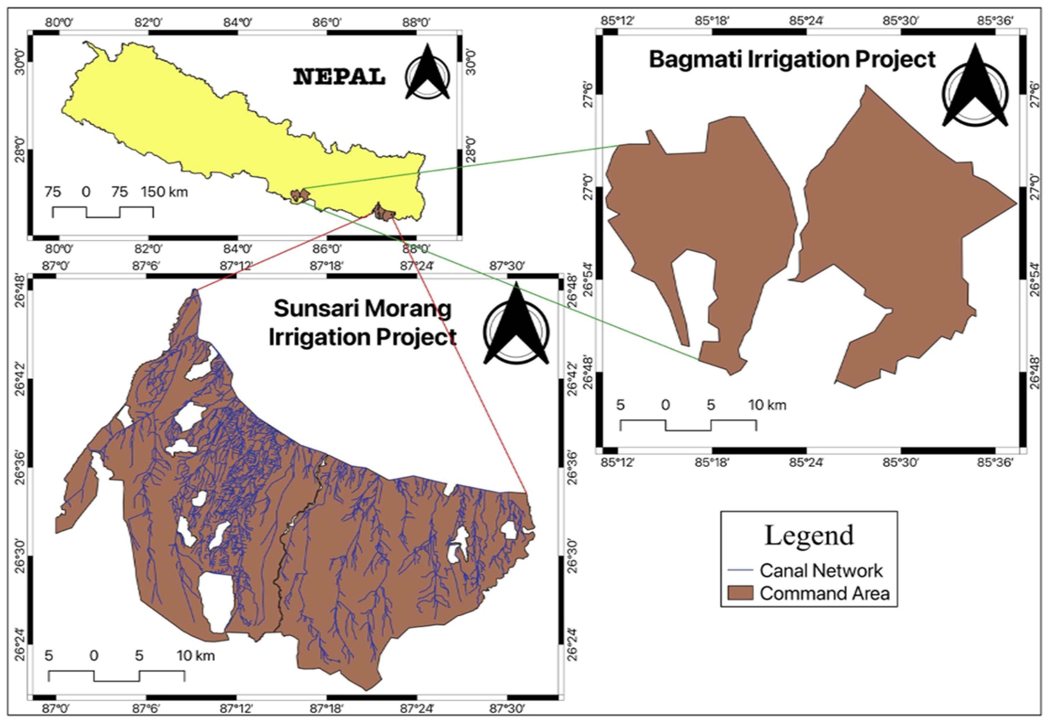
Figure 2.
General Overview of the study.
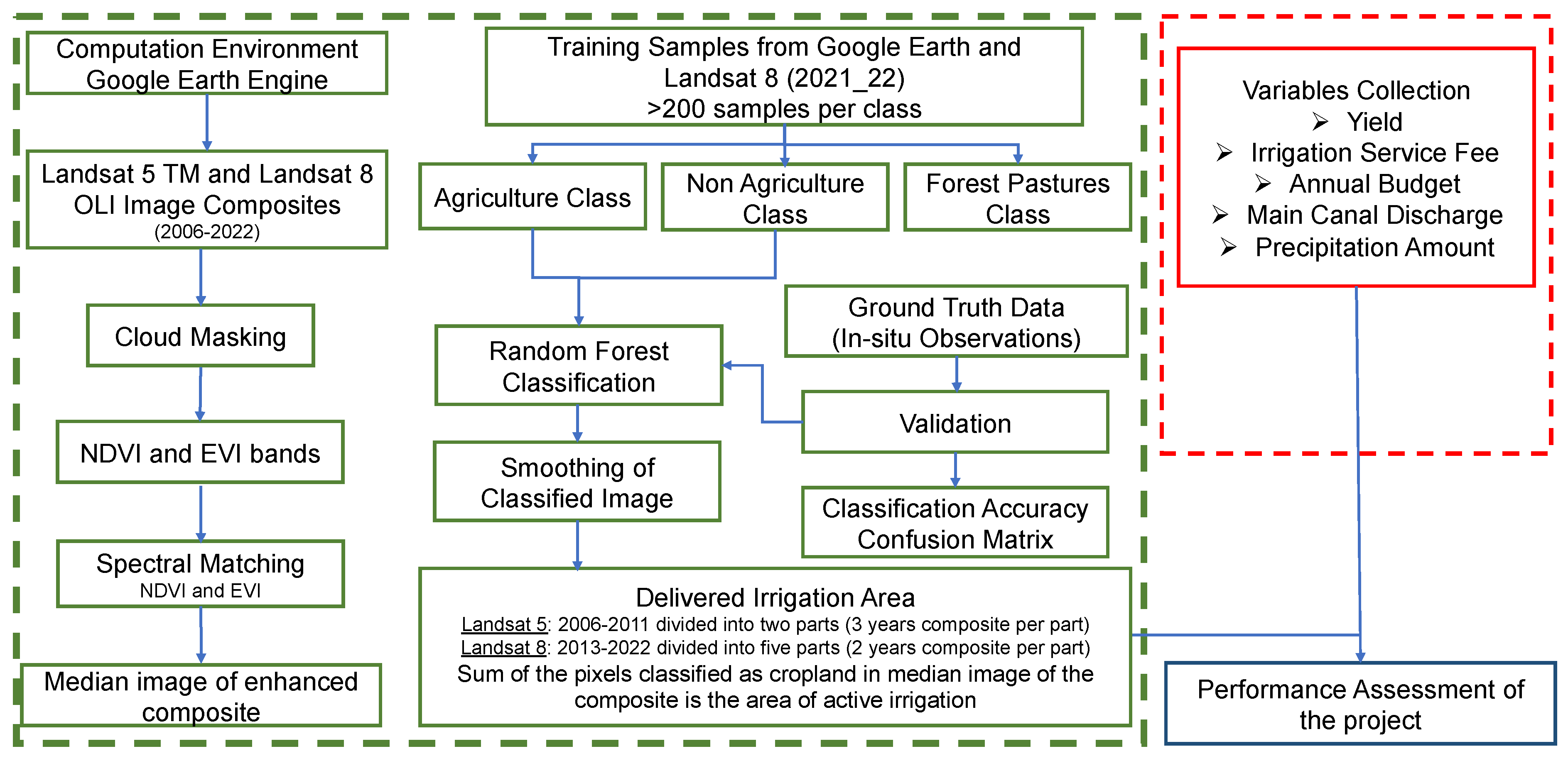
Figure 3.
Spectral Signature by class.
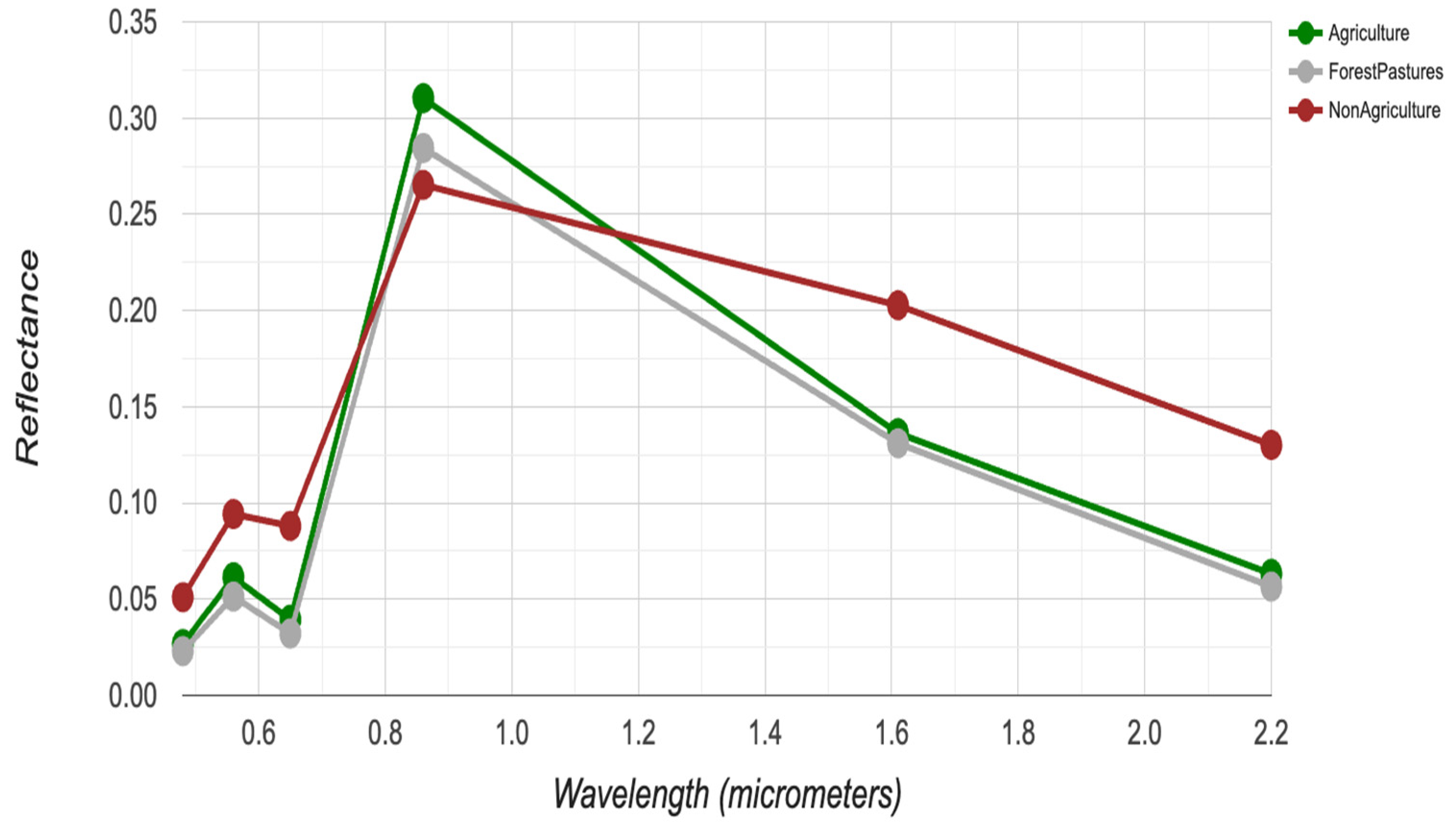
Figure 4.
Cropland Classification Maps of SMIP showing temporal changes in irrigated area from 2006-08 to 2021-22.
Figure 4.
Cropland Classification Maps of SMIP showing temporal changes in irrigated area from 2006-08 to 2021-22.
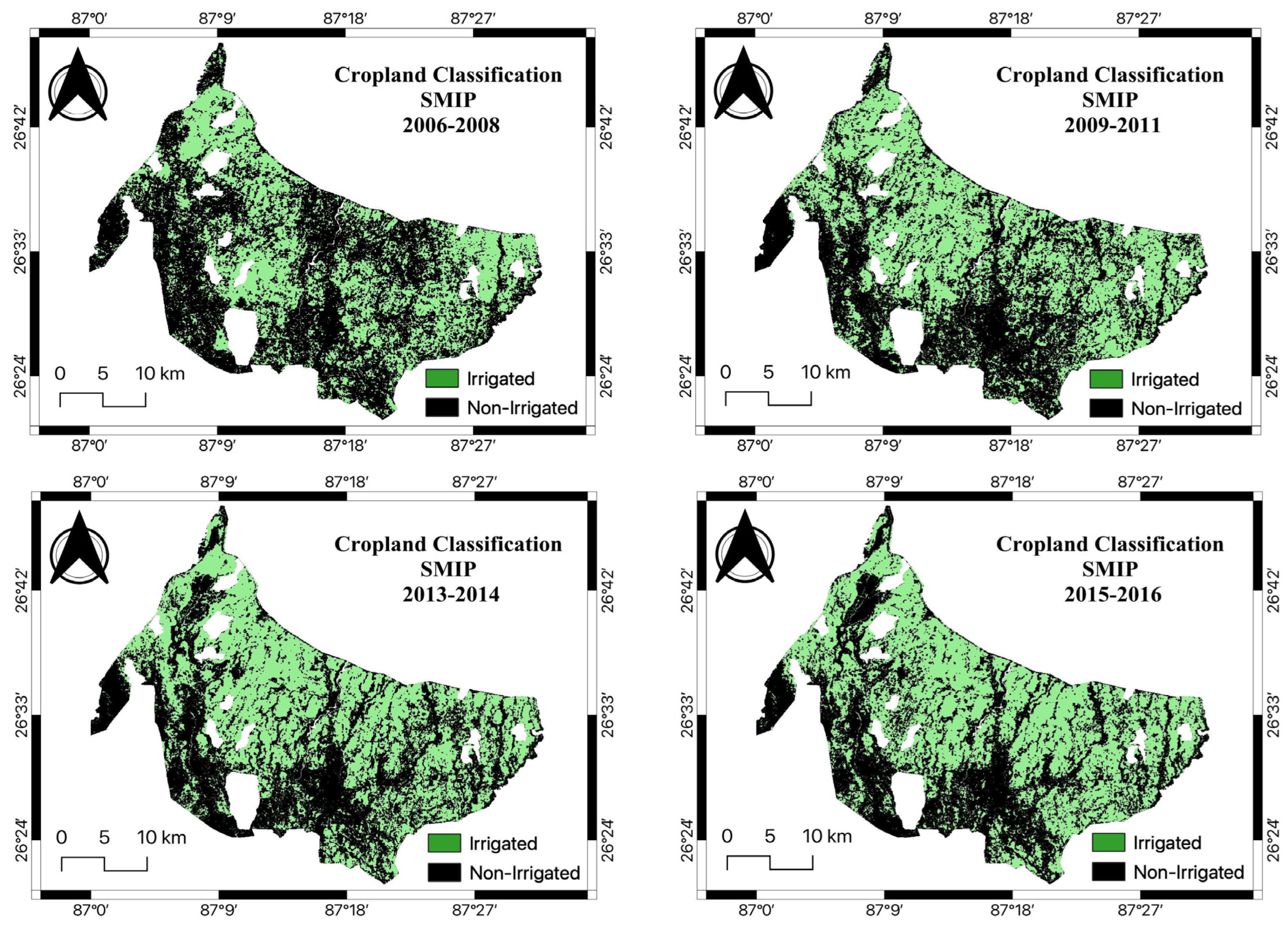
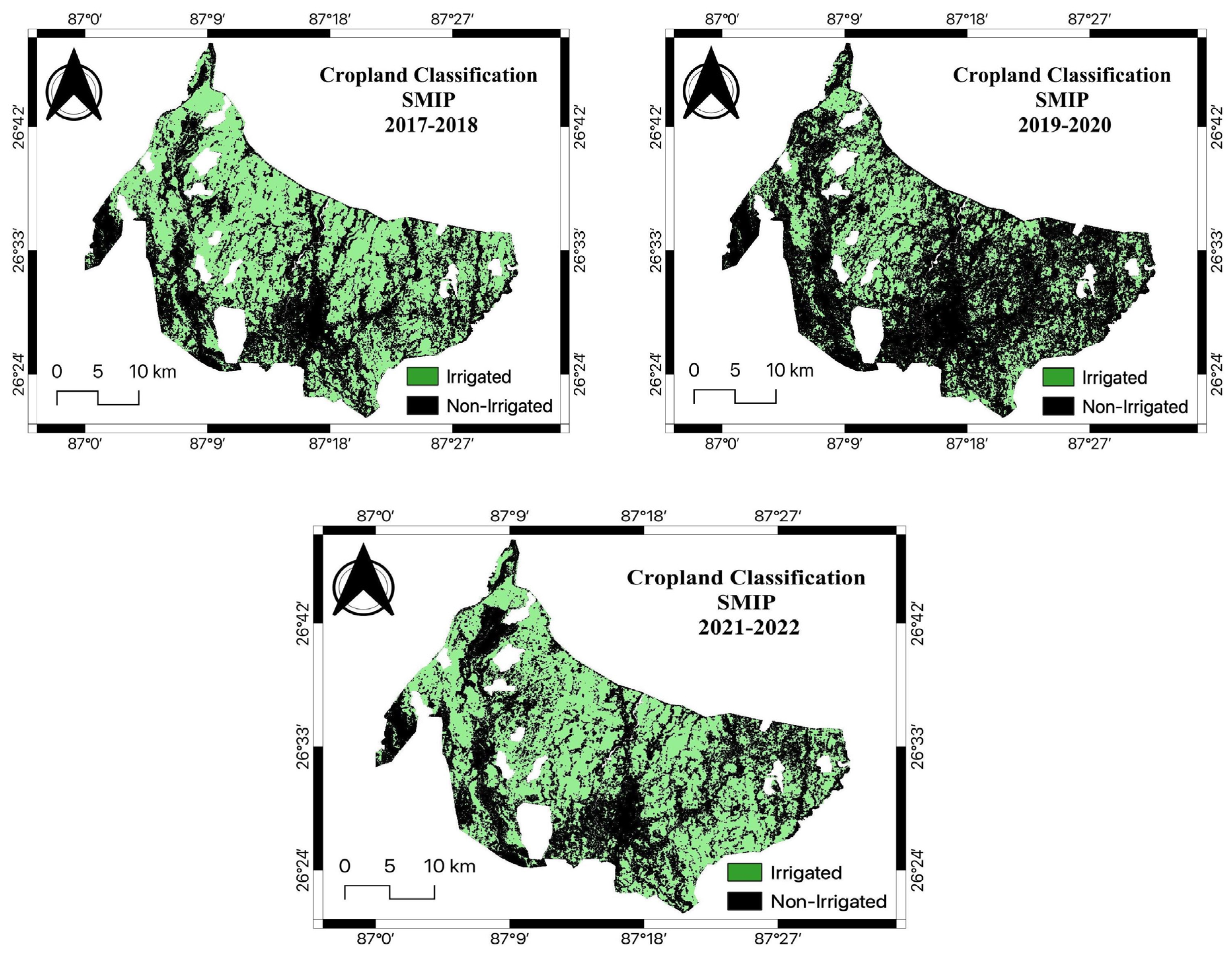
Figure 5.
Cropland Classification Maps of SMIP showing temporal changes in irrigated area from 2013-14 to 2017-18.
Figure 5.
Cropland Classification Maps of SMIP showing temporal changes in irrigated area from 2013-14 to 2017-18.
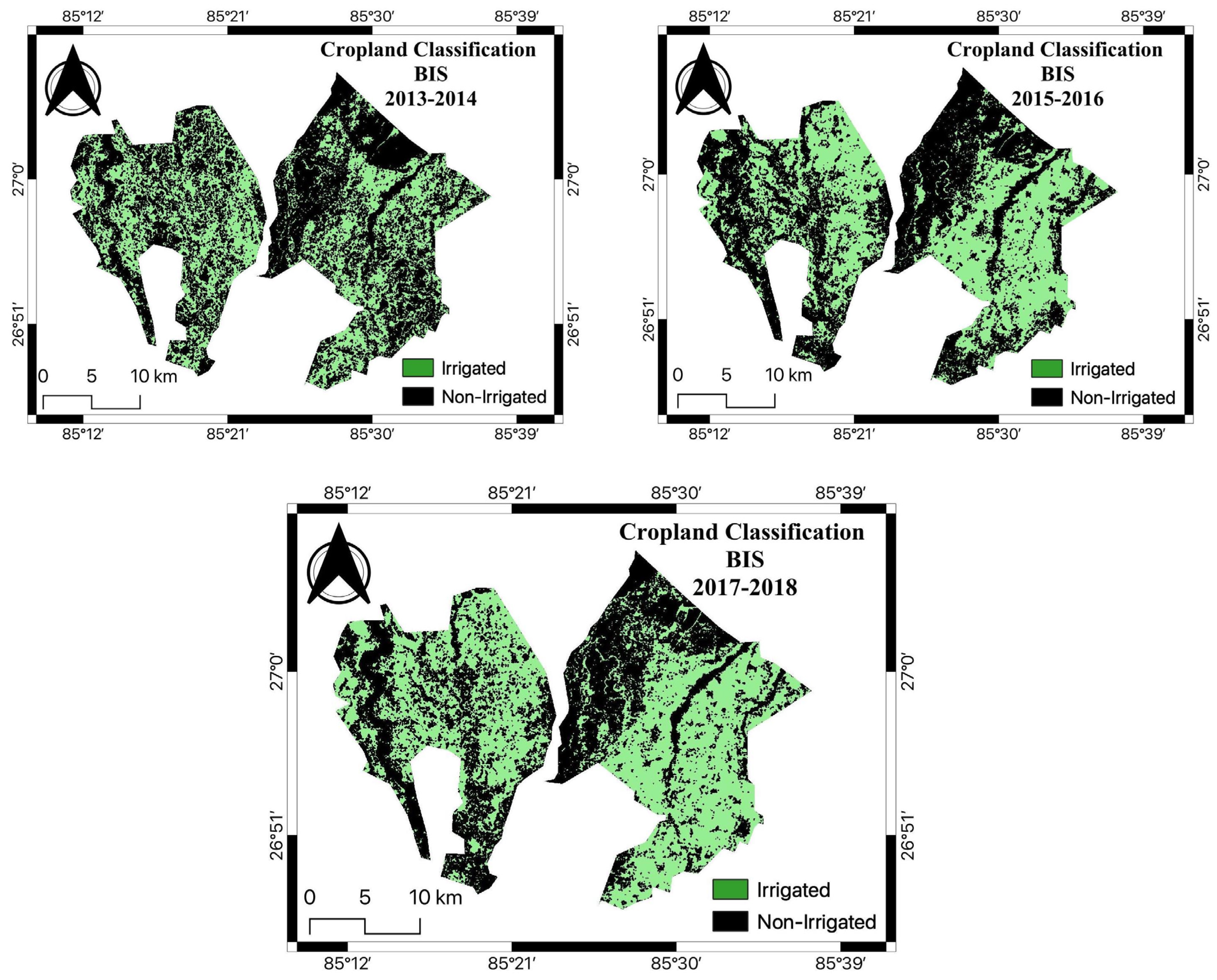
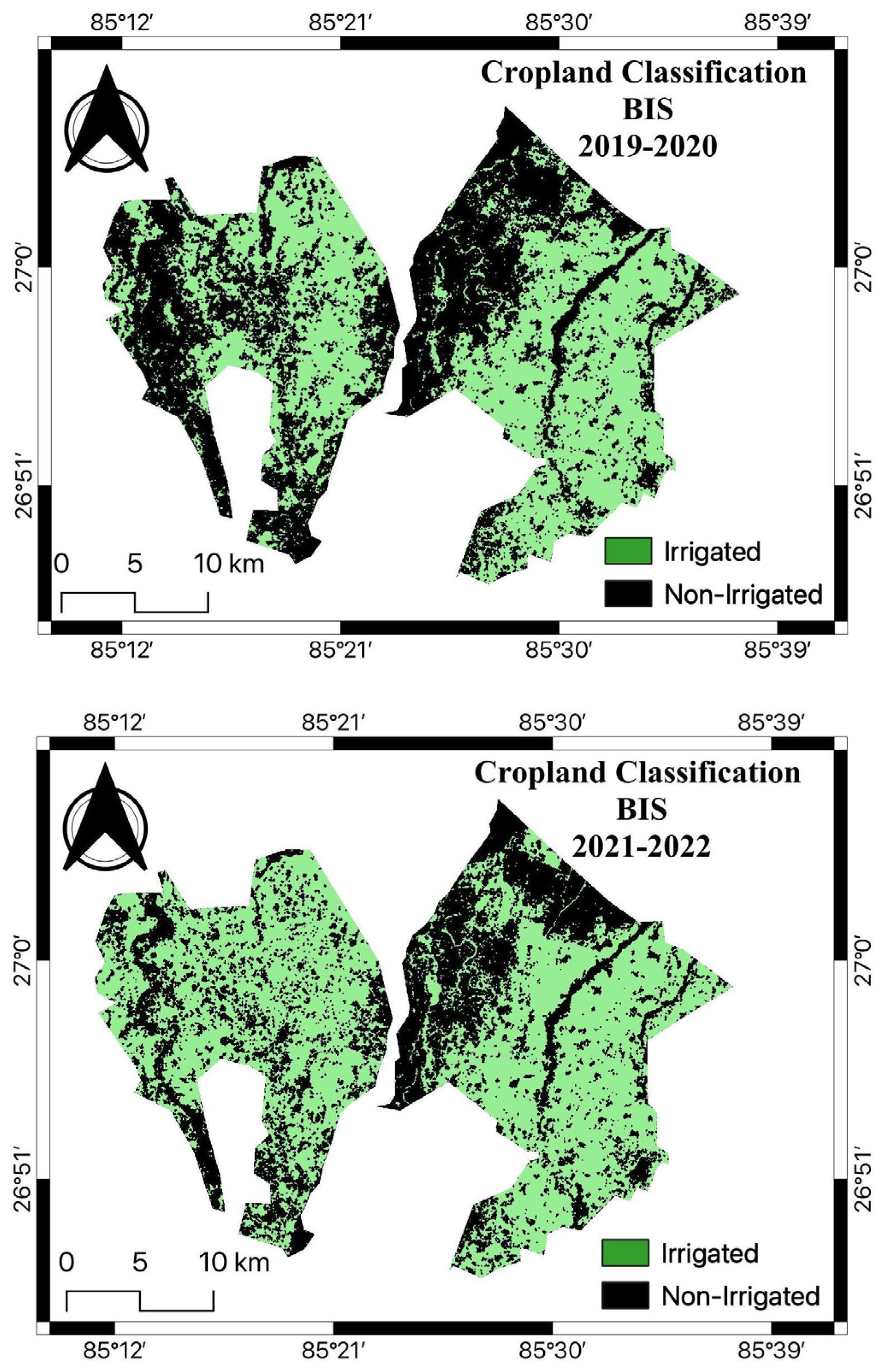
Figure 6.
Comparison of DWRI recorded and satellite derived irrigated area.
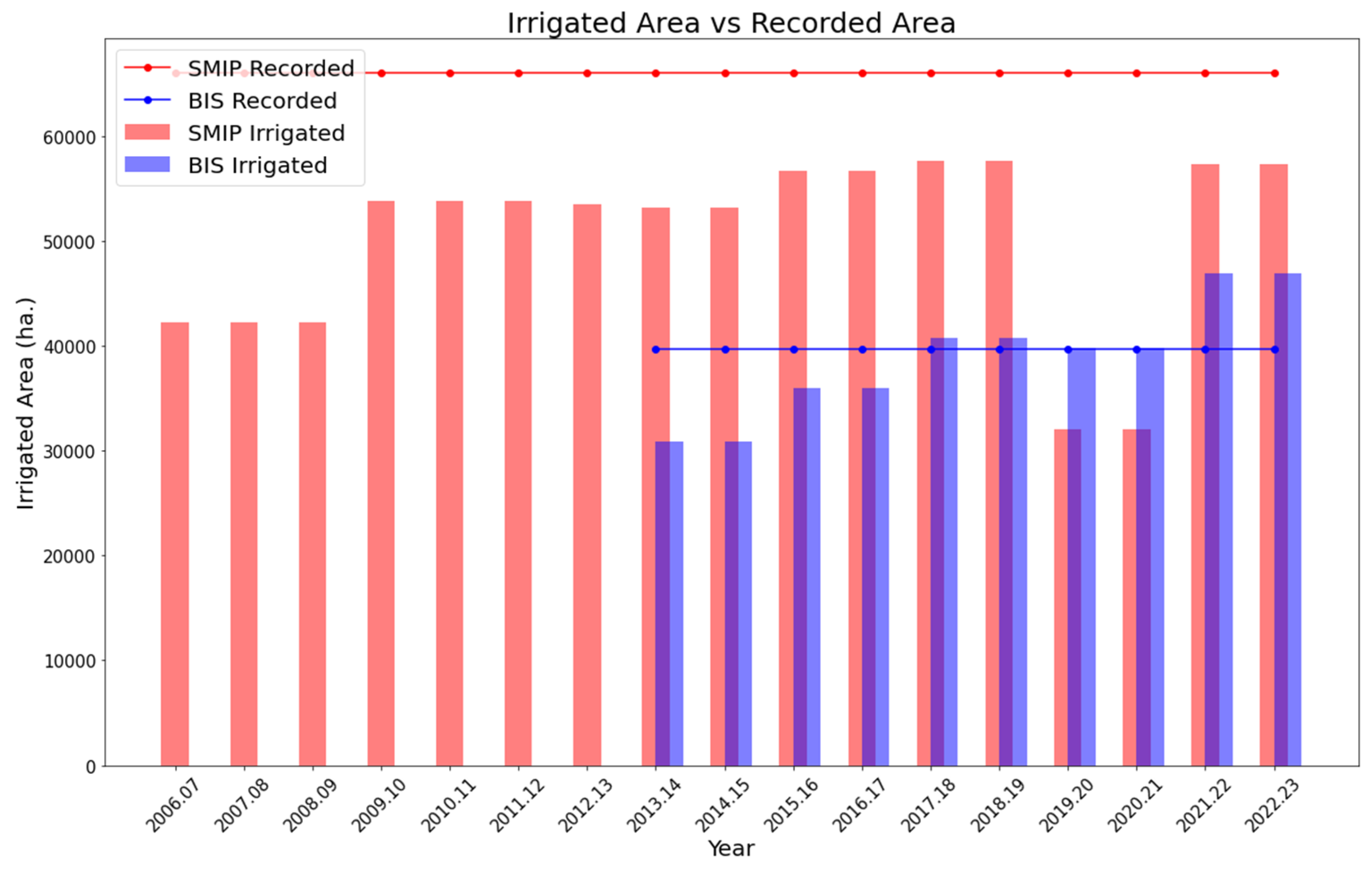
Figure 7.
Comparison of Global Cropland Classification Maps(GCCM) clipped for the study area (SMIP) with the Cropland Classification Maps obtained from this study throughout the study period; (a) 2006-2008; (b) 2009-2011; (c) 2013-2014; (d) 2015-2016; (e) 2017-2018; (f) 2019-2020.
Figure 7.
Comparison of Global Cropland Classification Maps(GCCM) clipped for the study area (SMIP) with the Cropland Classification Maps obtained from this study throughout the study period; (a) 2006-2008; (b) 2009-2011; (c) 2013-2014; (d) 2015-2016; (e) 2017-2018; (f) 2019-2020.
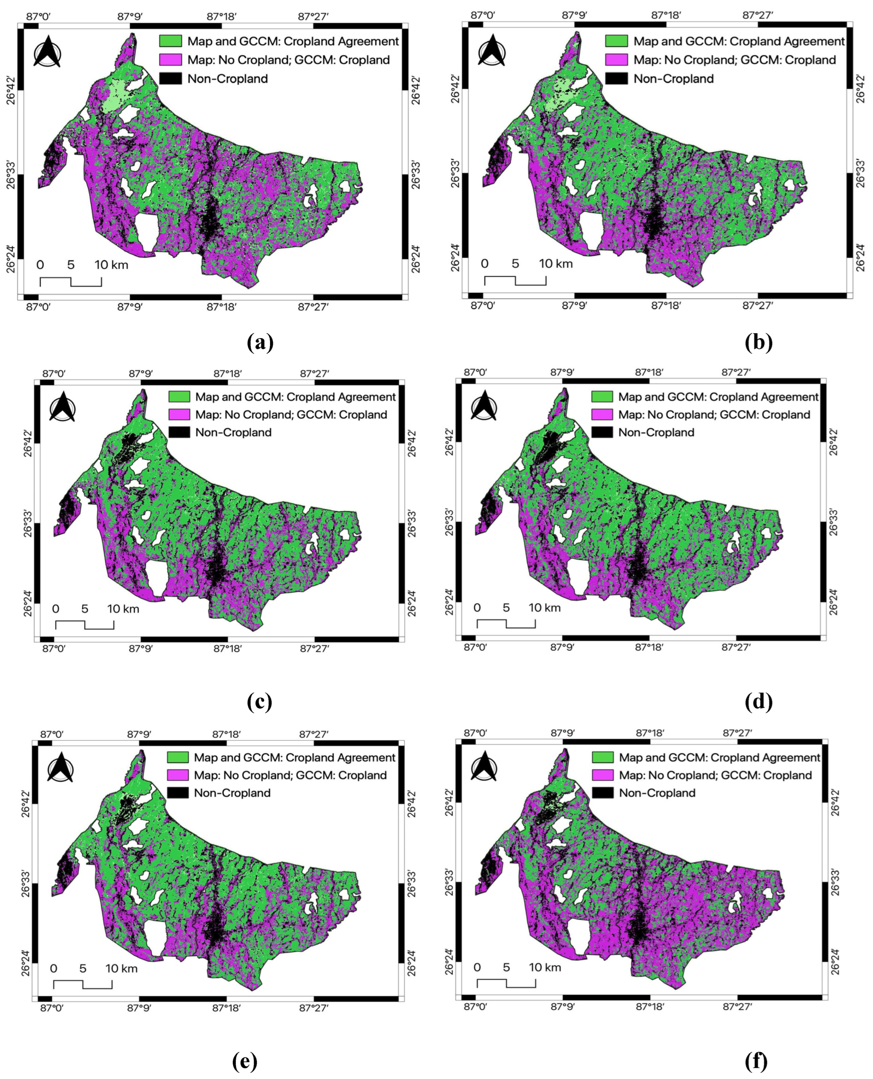
Figure 8.
Impact of Irrigated Area on Paddy Yield.
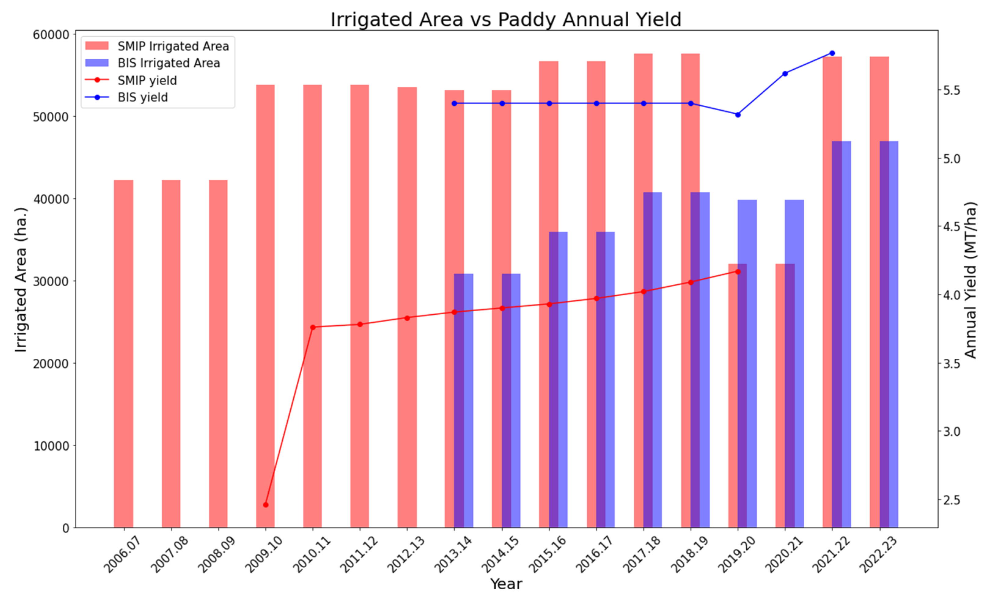
Figure 9.
Comparison of project annual yield with national average yield.
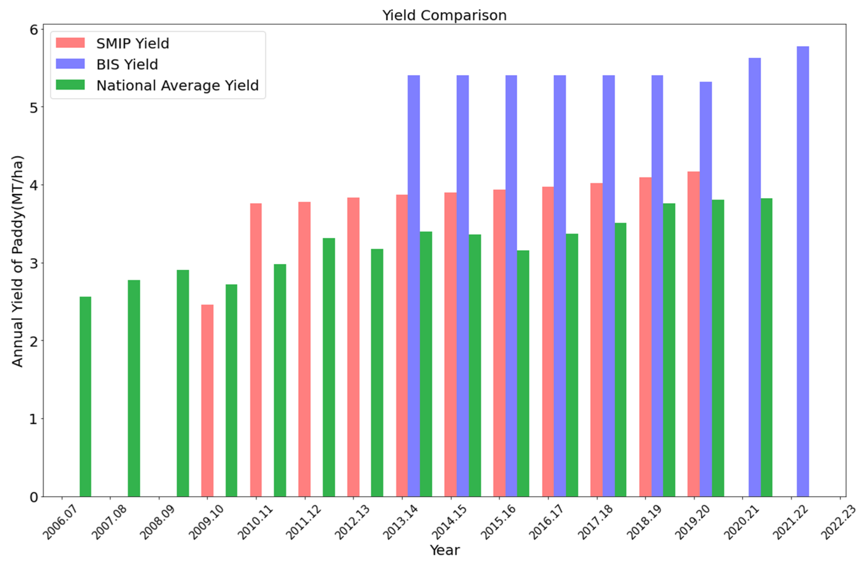
Figure 10.
Variation of ISF collection with Irrigated Area.
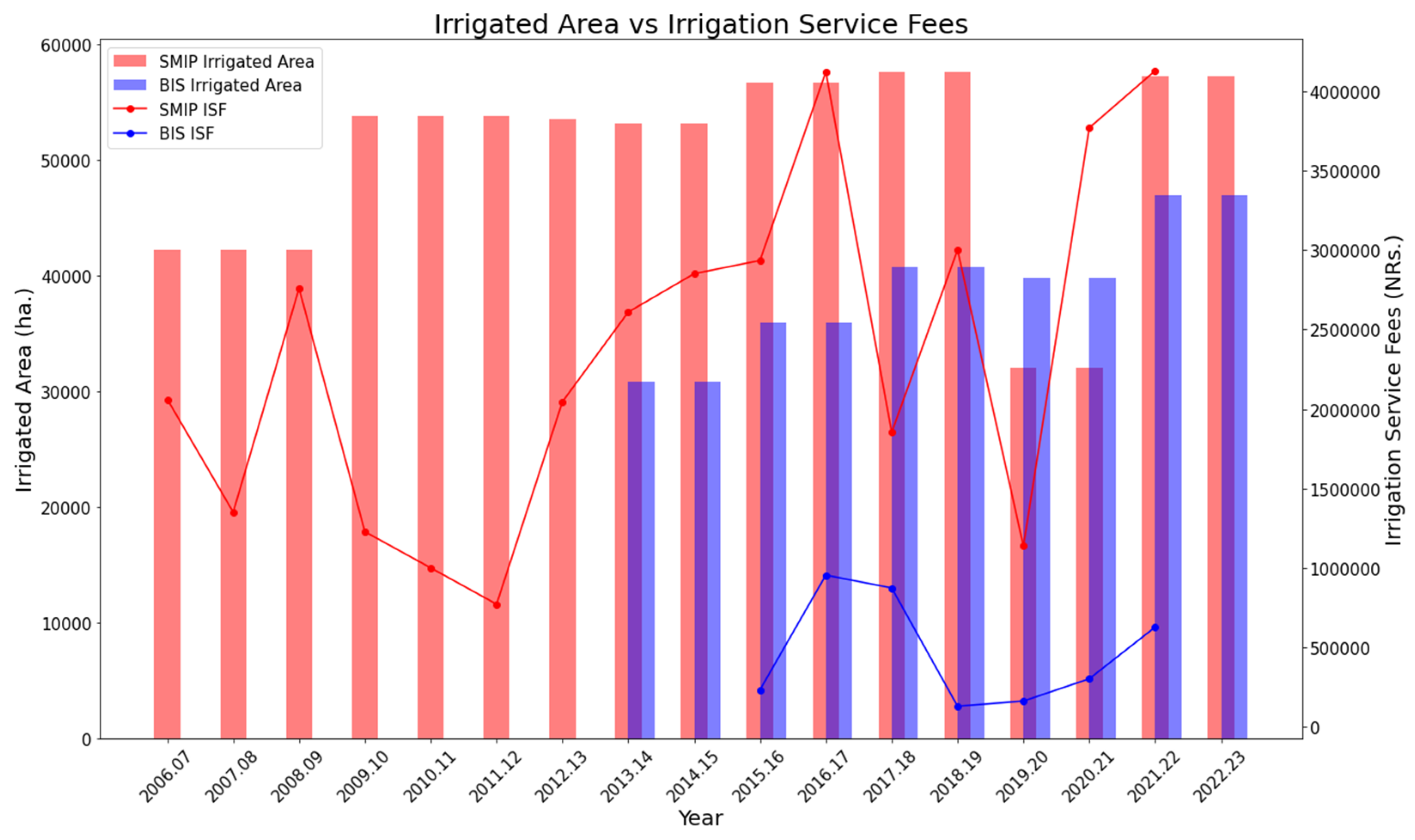
Figure 11.
Impact of project’s annual budget on Irrigated Area.
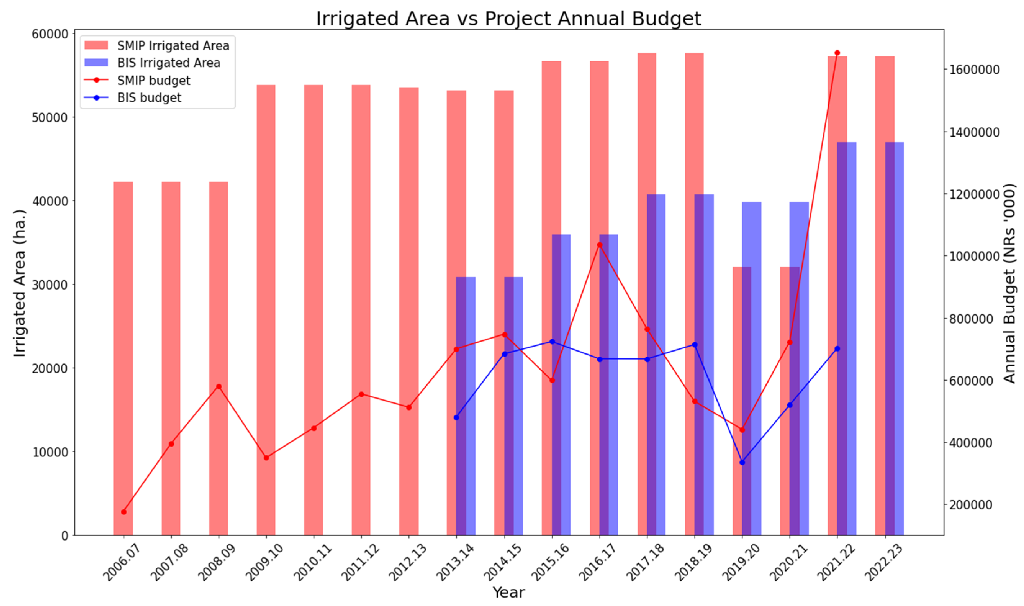
Figure 12.
Impact of discharge of main canal on Irrigated Area.
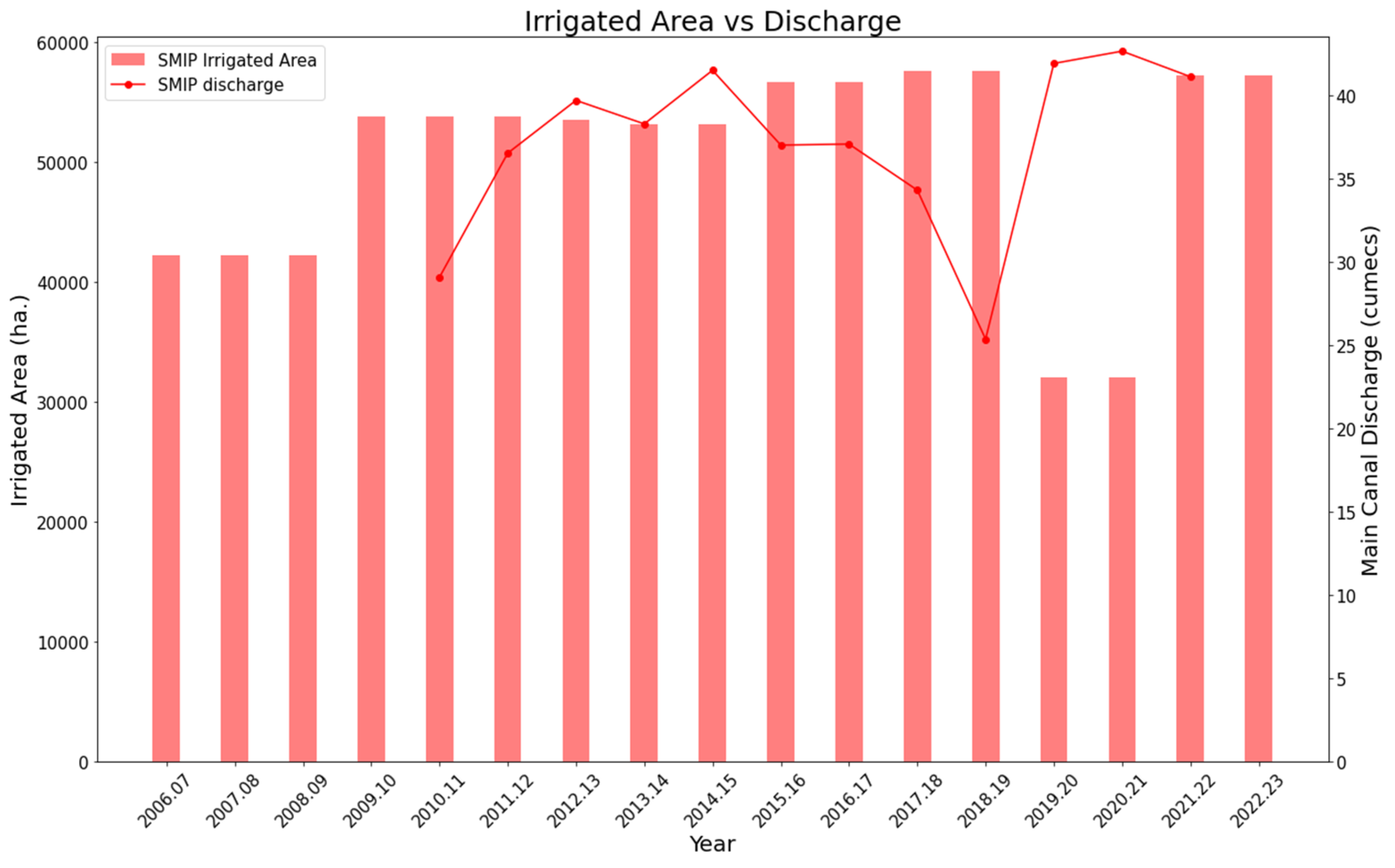
Figure 13.
Variation in precipitation amount with Irrigated Area.


Table 1.
Confusion Matrix.
| Predicted | ||||||
| Class | Agri | FP | Non-Agri | Total | PA | |
| Reference | Agri | 228 | 53 | 9 | 290 | 0.79 |
| FP | 9 | 125 | 5 | 139 | 0.90 | |
| Non-Agri | 1 | 22 | 104 | 127 | 0.82 | |
| Total | 238 | 200 | 118 | 556 | ||
| CA | 0.96 | 0.63 | 0.88 | |||
| OA | 82.2 | |||||
| Kappa | 0.72 | |||||
Disclaimer/Publisher’s Note: The statements, opinions and data contained in all publications are solely those of the individual author(s) and contributor(s) and not of MDPI and/or the editor(s). MDPI and/or the editor(s) disclaim responsibility for any injury to people or property resulting from any ideas, methods, instructions or products referred to in the content. |
© 2023 by the authors. Licensee MDPI, Basel, Switzerland. This article is an open access article distributed under the terms and conditions of the Creative Commons Attribution (CC BY) license (http://creativecommons.org/licenses/by/4.0/).
Copyright: This open access article is published under a Creative Commons CC BY 4.0 license, which permit the free download, distribution, and reuse, provided that the author and preprint are cited in any reuse.


