
Submitted:
25 July 2023
Posted:
27 July 2023
You are already at the latest version
Abstract
Extreme value analysis (EVA) is well-established to derive hydrometeorological design values for infrastructure that has to withstand extreme events. Since there is evidence of increased extremes with higher hazard potential under climate change, alterations of EVA are introduced for which statistical properties are no longer assumed to be constant but vary over time. In this study, both stationary and non-stationary EVA models are used to derive design life levels (DLLs) of daily precipitation in the pre-alpine Oberland region of Southern Germany, an orographically complex region characterized by heavy precipitation events and climate change. As EVA is fraught with uncertainties, it is crucial to quantify its methodological impacts: two theoretical distributions (i.e., Generalized Extreme Value (GEV) and Generalized Pareto (GP) distribution), four different parameter estimation techniques, (i.e., Maximum Likelihood Estimation (MLE), L-moments, Generalized Maximum Likelihood Estimation (GMLE), and Bayesian estimation method) are compared. Discrepancies due to the parameter estimation methods may reach up to 45 % of the mean absolute value, while differences between stationary and non-stationary models are of the same magnitude (differences in design levels up to 40%). Despite the underlying large methodological uncertainties, there is a robust tendency for increased DLLs in the Oberland region towards the end of this century based on the (non-)stationary models.
Keywords:
Extreme Value Analysis
; Design Life Levels
; heavy precipitation events
; stationary and non-stationary approaches
; Oberland
1. Introduction
In 2021, several parts of the world were affected by severe flooding due to heavy precipitation. Particularly China, India, and Western Europe suffered many casualties and high financial losses e.g., [1]. In July of the same year, Western Germany experienced exceptionally high rainfall rates of up to 200 mm from July, 13th to 15th, which exceeded the average monthly precipitation amounts, leading to the Ahrtal flood [2,3].
Often when such weather extremes happen, questions regarding the possible impact of climate change arise. Its influence can be suspected, but only detailed attribution studies enable the evaluation of reasoning such as climate change and human activity on individual events [2]. However, the long-term impact of climate change on the evolution of extremes can very well be examined [2]. The latest reports of the Intergovernmental Panel on Climate Change (IPCC) identified increases in the frequency and intensity of extreme precipitation in the past and projected further enhancements in the future e.g., [4,5]. For example, a heavy precipitation event that happened approximately just once every ten years in a pre-industrial world (1850-1900), is now likely to occur more often with a frequency of 1.3 times in ten years. In a future scenario with a 4°C warmer world than the pre-industrial state, the aforementioned event is even more likely to occur with an average frequency of 2.7 times in the same period of time [4]. This is in line with the thermodynamic law of Clausius-Clapeyron, according to which atmospheric moisture content exponentially increases with warmer temperatures resulting in higher precipitable water [4,6] and therefore in enhanced precipitation intensities if moisture availability is not a limiting factor [4,7].
A consequence of increased extreme precipitation would be a greater probability of flooding at regional scales, especially in mountainous and urban areas [4]. Hence, flood protection is an important topic in regions that are prone to flood hazards through heavy precipitation and new challenges regarding ongoing climate change require improved adaptation measures. To design protection measures appropriately, design values (commonly referred to as return levels (RL)) are calculated, which the structure must withstand [8,9,10].
Up to now the best available approach to estimate RLs is the extreme value analysis (EVA) [11], which aims to describe the stochastic behavior of a process at unusually large (or low) levels and hence makes presumptions about probable extreme levels in a certain future time period [11]. Since the presence or absence of individual extreme events of existing time series can confound the statistical representativeness of that time series for the corresponding region, a comprehensive database is necessary to reliably assess the return periods (RP) of the extreme values. In practice, this is often a limitation and becomes even more important, the higher the assumed return level is.
However, even if the time series is well representing the historical period, it is not necessarily representative of the future. One of the most frequently discussed topics is the lack of a possibility to capture changes in extremal behavior with traditional EVA [9,12,13]. If extremes tend to get more likely, a return period of an event from an earlier period can thus be much larger than that of the same event in a later period. This also has practical implications for engineering practice such as in hydrodynamic modeling based on heavy precipitation events to derive inundation maps and flood protection measures in the end [14].
With traditional EVA such changes in extremes cannot be considered since only one return level is calculated representing the whole time series. Therefore, the question arises whether traditional methods are still adequate or whether new statistical methods should be developed to account for potential changes in (future) extremes. Hence, many studies applied a new concept referred to as non-stationary extreme value analysis (non-stationary EVA). In contrast to traditional (i.e., stationary) EVA, it is assumed that the statistical properties of time series change, which enables the consideration of alterations in extremes through climate change or – especially in the context of flooding – other (human) interventions such as land cover change, urbanization, or river regulation [10,15].
Following the definition of stationarity of Coles [11], in a non-stationary time series properties of the distribution function is enabled to shift over time. These changes can emerge in different ways. The most apparent one would be a linear trend in the mean of the variable but also shifts in the variance or step changes could be possible. However, despite the general agreement on altering means and extremes of precipitation, evapotranspiration, and rates of river discharge [4], there is no consensus about the usage of non-stationary EVA [9,10]. Since it is virtually impossible to know the true underlying statistical characteristics of hydrometeorological time series [11], there is often no plain distinction between whether a times series can be called stationary or non-stationary. Random fluctuations or deviations from the mean are to be expected even in stationary time series [16] and the sample can also be part of a cyclical climate variability [17]. Therefore, the future state may be stationary but just different from the one before [18,19]. Matalas [18] denote the maintenance of non-stationarity in form of a trend into the future to be problematic since it is unsure whether an apparent trend in the past is indeed an indication of non-stationarity [16,18,20] and thus can be extrapolated into the future without ‘catastrophic consequences’. Hence, several studies recommend the use of the non-stationarity assumption only when changes can be predicted due to the knowledge of underlying physical drivers [20,21].
In case non-stationary EVA is applied inappropriately (especially to short time series) this may increase the uncertainties, and thus stationary EVA should be better used by default [21]. Furthermore, there is also no agreement on the methodology of non-stationary EVA [9]. This is mainly because typical concepts of return period and return level no longer provide distinct values in the non-stationary case [22,23]. Alternative concepts have been developed such as the design life level and minmax design life level from [24], the approaches of expected waiting time until a given exceedance occurs, or the expected number of events over the return period [23] as well as equivalent reliability by Hu et al. [25].
In this study, one stationary and three non-stationary statistical models are checked for their robustness in deriving DLLs of precipitation extremes. In order to allow for a direct comparison between stationary and non-stationary methods, a rather simple but effective approach based on design life level was developed. For the assessment under stationary (non-stationary) conditions, method-inherent uncertainties are quantified by using two (one) theoretical extreme value distribution(s), and four (three) parameter estimation methods. It is expected that a quantification of the method-inherent uncertainties under current climate conditions will allow a more robust assessment of precipitation extremes under future climate conditions. Moreover, it is analysed how regional climate models (RCMs) can be capitalized to derive future DLLs. Results are compared to extrapolated EVA results based on observed precipitation data.
2. Materials and Methods
This section introduces the study region as well as the data and methodologies applied in this study.
2.1. Study Region
The study area mainly comprises the Oberland region of the federal state Bavaria in the south of Germany (Figure 1). More precisely, the Oberland region includes the districts Bad Tölz-Wolfratshausen, Garmisch-Partenkirchen, Miesbach, and Weilheim-Schongau. The topography of the study area is characterized by the flatter alpine foothills in the north of the region and alpine areas in the south. Following the elevation gradient in the study region, the distribution of precipitation reveals higher mean annual sums in the south than the north [26]. Besides the annual amounts, extreme precipitation events can occur due to different prevailing weather situations in the region, mainly due to the blockage of northerly flows of humid air masses at the northern edge of the Alps, often referred to as the so-called Vb-cyclones [27], and due to deep convection, partly triggered by the mountainous terrain of the Alps [28].
Moreover, it has been shown that the precipitation patterns have undergone significant changes, most likely due to global climate change [26]. Thus, although the Oberland region comprises a relatively small region (in Germany), it may serve as a blueprint for larger regions with complex orography, complex precipitation regimes, and regions that are already affected by climate change.
2.2. Data
Across the study area, there are 24 observation stations available with sufficiently long time series of daily precipitation data, i.e., a minimum of 30 years is required for EVA of 100-year return periods. However, as it requires a very long time series to investigate possible changes in statistical characteristics for non-stationary EVA [21,29], even stations with less than 50 years were neglected, which resulted in a total of 16 stations. For stationary EVA, all 24 stations were explicitly taken into consideration because it is one of the objectives to demonstrate how the applied methods perform in relation to the length of the time series. Figure 1a shows the spatial distribution as well as the length of the observed time series of those 24 stations. Stations with less than 50 years of data are marked with red dots. 16 stations have time series longer than 50 years and 13 stations longer than 70 years.
Besides station data, high-resolution RCM model simulations have been used in this study to derive return levels (see Table 1). In particular, outputs from Coordinated Downscaling Experiment - European Domain (EURO-CORDEX) at a horizontal grid spacing of 0.11° (EUR-11, approx. 12 km) have been applied [30,31]. Due to computational resources, we restricted our analysis to CORDEX experiments based on the regional model COSMO-CLM, nested into three different general circulation models (GCMs) from the Coupled Model Intercomparison Project phase 5 (CMIP5) [32]. Those are the EC-Earth from EC-Earth Consortium Europe, the CNRM-Cerfacs from the Centre National de Recherches Météorologiques, and the MPI-ESM-LR from the Max-Planck-Institute for Meteorology. Three realizations were available for MPI-ESM-LR (r1, r2, r3) and EC-Earth (r1, r3, r12), which only differ in their initial conditions [33,34]. Each future scenario simulation is assigned the same realization integer as the historical run from which it was initiated [34]. For future scenarios, the high-emission scenario RCP8.5 with 8.5 radiative forcing in 2100 was chosen. As can be seen from Table 1, historical simulations are available for approximately the period 1950–2005 and future projections for the period of 2006–2100. Since an initial comparison of statistical properties with the observations is needed, local information from the climate data for the position of the above-mentioned stations is assessed. Therefore, the time series of the grid cells corresponding to the location of the stations have been extracted. It is noteworthy that the utilized RCM simulations have been bias-corrected [35] for specific EVA models (i.e., N2 and N3). For other assessments, only the (relative) climate change signal has been needed rather than the intensity-corrected time series. In these cases, the delta change approach has been followed.
2.3. Methods Applied for Extreme Value Analysis (EVA)
Over the last five decades, EVA has emerged as one of the most important statistical disciplines for applied sciences [11]. In general, EVA is applied to estimate the stochastic behavior of a process at more extreme levels than already observed [11,36]. It is of great interest since in many disciplines knowledge about possible future extreme cases is necessary [11]. This extrapolation to more extreme or less likely events is done by fitting a theoretical distribution function () to the selected subset of extremes and deriving a value which – according to this – would occur with a certain small probability [8,11]. The accurate estimation of these tails is in general challenging since there is usually only little data to fit the theoretical model to the sample distribution [11]. Consequently, this can lead to large uncertainties in the derivation of design levels, especially of low occurrence probabilities [21].
Figure 2 is giving an overview of the data and methodologies and will serve as a guide through the workflow of stationary and non-stationary EVA.
2.3.1. Theoretical Extreme Distribution Functions
There are different model families whose distribution functions are appropriate for modeling extreme events [11]. Only the two most common ones were used in this study. Firstly, following the block maxima approach, the distribution of annual extremes (AMAX) converges to the Generalized Extreme Value (GEV) distribution, whose cumulative distribution function is expressed as follows:
The GEV combines three limiting distribution functions namely Gumbel, Fréchet, and Weibull into one family [37,38]. The function depends on three distribution parameters which allows the flexibility to model different characteristics of extremes: the first one is the location parameter indicating the center of the distribution, the second is the scale parameter representing the size of deviations around the location parameter, and the third is the shape parameter which controls the tail of the distribution function [11,38]. An often-mentioned side effect of the block maxima approach is the neglect of second highest values within the defined blocks [9,11]. This is different from the threshold approach - often called peaks over threshold (POT) – where extreme events above a selected threshold are used for EVA. Because of the larger sample of extremes extracted from the historical data, most studies expect an improvement of estimation of design levels using POT [9,11,39]. It is also recommended for relatively short time series or time series with the infrequent occurrence of extremes and requires higher resolution of the basic time series, i.e., hourly, or daily observations [9,11,40]. Just as the GEV remains an appropriate model for the AMAX, for a large enough threshold u similar arguments suggest that the generalized Pareto distribution (GP) is appropriate for the selected threshold excesses [11,39]. The cumulative distribution function can be expressed as follows [11,41]:
There is a relationship between the GEV and GP distribution where the GP is approximately the tail of the GEV [11,42]. The scale parameter of the GP is a function of the parameters of the corresponding GEV : . The shape parameter of the GP distribution is equivalent to that of the corresponding GEV distribution [39], which makes invariant to block size, while is unperturbed by the changes in and which are self-compensating [11]. So just as the shape parameter is dominant in determining the qualitative behavior of the GEV , it is analogous for the GP [11]. An important intermediate step of the POT approach is the choice of an appropriate threshold, which should on the one hand be high enough to minimize the bias due to the asymptotic tail approximation and on the other hand be low enough to obtain a sufficient sample size in order to keep parameter estimation uncertainties as low as possible [9,43,44]. There are already several approaches to setting a threshold, of which Scarrott and Macdonald [43] have provided a comprehensive review. Since classical threshold selections are not efficient and rather time-consuming, when many datasets are analyzed, a relatively simple, but also frequently utilized approach was implied in this study, which uses percentiles of precipitation data [39,45]. Therefore, in the first step for each station, the percentile of all rain day amounts was used as a threshold and adjusted if the resulting sample size did not lie within the range of one to two times the length of the AMAX sample size [45]. In addition, since extremes over a threshold tend to cluster and thus induce serial dependence [11], a declustering approach was applied following Coles [11].
2.3.2. Parameter Estimation Methods
In the stationary case, both GEV and GP distribution functions were used for fitting and parameters were estimated with four different parameter estimation methods (PEM) which are Maximum Likelihood Estimation (MLE), L-moments, Generalized Maximum Likelihood Estimation (GMLE), and a Bayesian approach. The MLE approach became one of the standards in statistical inference because of its asymptotic efficiency with sample size n increasing to infinity and for distributions satisfying several regularity conditions [11,46,47]. Meanwhile, it is one of the most frequently applied methods to estimate unknown parameters and in addition one of the most flexible regarding its application to modified models [11]. As a likelihood-based approach, MLE yields to find the parameter values of which maximize the probability of resampling the sample data [8]. Coles [11] provides a detailed description of the MLE method. According to Coles and Dixon [48] maximum likelihood estimators for the AMAX approach tend to get unstable for sample sizes of . In addition, Hosking and Wallis [49] showed for the GP, that unless the sample size is 500 or more, estimators derived by the method of moments are more reliable than MLE. There are several variations of the method of moments with probability-weighted moments and L-moments being one of them [9]. Since L-moments are more robust to outliers than conventional moments and additionally enable more secure inferences about the underlying probability distribution to be made from small samples [50], this technique is often the preferred choice. Thereby, parameter estimation with L-moments is similar to the common method of moments, but convenient moments are replaced by L-moments, which are expectations of certain linear combinations of order statistics [50]. For detailed information, Hosking [50] unified the theory of L-moments and provides guidelines for practical use. Another method invented to circumvent possible weaknesses of the MLE is the GMLE [51], which restricts estimates of the shape parameter . Since maximum likelihood estimates can generate absurd values of the GEV shape parameter , when sample sizes are small [50,51], with GMLE a prior distribution is chosen assigning weights to different values of within the allowed range. The choice of prior function is by default the beta distribution similar to Martins and Stedinger [40], Martins and Stedinger [51]. Analogous to the MLE method, the estimator of can be identified by maximizing the generalized log-likelihood function [51] which is the joint distribution of the likelihood function and the prior distribution. As an alternative to classical statistical inference, the last estimation technique used is based on Bayesian inference [46]. One of the main differences is that parameters are no longer assumed to be constant but are rather treated as random variables with distribution function [11]. This is called prior distribution since it contains possible beliefs about without reference to the data [11]. An obvious advantage of this method would be the inclusion of additional knowledge about the parameters which may come from other data sets or a modeler’s experience and physical intuition [46]. On the other hand, choices of priors remain subjective decisions, so different analysts would supposedly specify different priors [11]. By applying the well-known Bayes’ Theorem, the prior distribution can be converted into a posterior distribution , which includes the additional information provided by the data x, as follows:
But the normalizing integral in the denominator aggravates the direct computation of the posterior distribution [11,36]. This difficulty was overcome by the development of simulation-based techniques, such as Markov Chain Monte Carlo (MCMC), which facilitated the use of Bayesian techniques to the extent that they are now standard in many areas of application [11]. After fitting the statistical models, consistency between modeled distribution and distribution of the sample was done by the examination of diagnostic plots such as quantile-quantile plots (QQ-Plots), probability plots, and simple comparisons of density distributions as well as the Kolmogorov-Smirnov test (KS-test) as a goodness-of-fit test [13,38,39,52].
2.3.3. Implementation of Non-Stationarity
There already exist multiple options to include non-stationarity into EVA [12,13,24,52] which usually have a time dependency of the probability density functions in common [12]. Several of them simply added a linear link function relating the distribution parameters to explanatory variables [23,24,38,52], but some utilized more complex structures such as cubic splines [12] or quadratic trends [53]. The latter as well as other smoothing techniques indeed provide good fitting and flexibility to the data, but, on the other hand, are sensitive to unforeseen evolution of the temporal pattern of the variable [12] and therefore difficult for extrapolation. Assuming a linear trend, therefore, seemed natural and useful as a starting point [24]. However, to check whether there is a justification for non-stationary assumptions, time series were examined for trends using the non-parametric Mann-Kendall trend test [38,52]. Detection of trends or detailed exploratory data analyses (EDA) are critical issues regarding non-stationary EVA as they can have a considerable effect on the results and facilitate the later interpretation [21,52]. Due to technical reasons, non-stationarity has been considered only for the AMAX approach and the MLE, GMLE, and Bayes estimation methods in this study. Furthermore, in this study, only linear dependencies for the location and scale parameter have been included, as the estimation of the shape parameter is already under stationary assumptions the most difficult one and requires long-term observations that are in practice often not available e.g., [11,22,38,52]. As suggested by many studies, the logarithm of the scale parameter was used to ensure positive values [22,52]. In addition to the stationary model S1, the following three non-stationary models were implemented:
- 1.
- N1: non-stationary model (1) with location parameter being a function of time: (t) = + t
- 2.
- N2: non-stationary model (2) with location parameter being a function of annual precipitation: (t) = + P
- 3.
- N3: non-stationary model (3) with location parameter being a function of annual precipitation and parameter being a function of time: (t) = + P, ln((t)) = + t
These non-stationary models were adapted from Šraj et al. [52], but slightly changed for model N3 not only being dependent on time but rather a mixture of precipitation and time. Time as a covariate should be treated with caution because changes in the past are not automatically the same as in the future, especially for periods longer than ten years into the future [52]. An advantage of employing climate variables such as annual precipitation as a covariate is that climate model predictions or projections can then be employed as covariates to estimate future change which makes the proposed model more practically useful [10,52]. As recommended by Gilleland and Katz [42], covariate vectors (time and precipitation) were scaled to zero. To check whether the inclusion of the certain covariate into the model was significant and to indicate the best fitting statistical model the Akaike information criterion (AIC) and the deviance information criterion (DIC) were applied for MLE/GMLE and Bayesian estimation method, respectively [52]. In both cases, models with the smallest AIC or DIC value indicate the best model performance [54]. In addition, for MLE and GMLE a likelihood-ratio test (lr-test) was performed to test the significance of the inclusion of covariates into the models [52].
2.3.4. Equivalent Design Life Level
Since for non-stationary EVA the term return level becomes ambiguous, the concept of design life level (DLL) by [24] was used and further developed as an equivalent Design Life Level. Since the DLL is defined by the risk of exceedance in a certain time span, a connection between DLL and RL can be established through the common term of hydrological risk. For an n-year RL the hydrological risk can be computed for the same time period as used at the computation of DLL and by equating the risks, an equivalent DLL can be computed that has the same risk of exceedance as the associated RL. For a 10-year level and a time period of 30 years, the hydrological risk R would be , and analogously for a 100-year level . In this study, historical DLL were computed for the time period 1971–2000 and future DLL for 2071–2100. Extrapolation of non-stationary models, i.e. the models N2 and N3, requires a vector of the covariate in this future time period. For time as a covariate, this is a trivial derivation, but for annual precipitation as a covariate, climate model projections are necessary. Due to the partly strong deviations between modeled and observed annual precipitation in the RCM projections, the RCM annual precipitation was adjusted by using a linear transformation of the mean and the standard deviation between the historical model simulations and the observations . Applying it to the future model simulations , transformed future simulations are then derived as follows:
2.3.5. Usage of Regional Climate Models
RCMs potentially provide an opportunity for EVA in the absence of (sufficient) observation data, not only regarding the length of the time series but also their spatial distribution. In this context, we explore the general usability of RCMs by comparing the EVA results to those based on the observations. First, the regional climate data has been validated by comparing the distributions of precipitation from the observation stations to those of the corresponding RCM grid cells. Therefore, different approaches were followed, such as the visual inspection of boxplots (and especially deviations in the median) as well as Kolmogorov-Smirnov (KS) tests to compare the distributions of modeled and measured AMAX. Besides the extrapolation of design levels from observations into the future (see models N2 and N3), climate models provide an additional possibility to derive information about future extreme behavior. Since RCM simulations used in this study were not bias-corrected per se (only for N2 and N3), projected DLLs were calculated with a simple and frequently used approach, called delta change method e.g., [55,56,57,58]. It differs from other bias correction methods as it does not adjust RCM simulations itself but uses the combination of observations and only the RCM change signal [57,58]. In that way, differences, i.e., the change factor or the ‘delta’ between the design level of the future (2071–2100) and historical simulations (1971–2000) were calculated and then added onto design level from observations .
It has to be mentioned, that confidence intervals of the delta approach are symmetric which does not represent the asymmetry that is generally associated with quantile estimators of extremes [22]. Since this approach is not always physically consistent and can attain negative values for the lower limit, it should be interpreted with caution [21].
3. Results
3.1. Theoretical Distributions and Parameter Estimation Methods
After modeling the extreme behavior using the GEV and GP distributions for the above-mentioned stations in the Oberland region, the fit of the estimated models was evaluated. In principle, according to KS-test only for a few stations the modeled distribution did not fit the data very well. In particular, for station 2759 all estimated GEV models showed poor performance of the fitting. Also, the QQ-plots confirmed that distributions do not agree very well. In addition, for stations 2724 and 2903 model fit was also poor when using the GEV distribution and GMLE and Bayes estimation. They seem to have experienced more extreme events than were modeled by the distributions. These stations should therefore be interpreted with care in the following sections. In the next step, parameter estimates are examined in more detail with regard to the four estimation methods, i.e., MLE, GMLE, L-moments, and Bayesian estimation method. Relative differences between the estimation methods were the largest for the shape parameter. In the case of AMAX, the variation coefficients of the shape parameter compared to those of the location parameter were approximately 50 times larger, and with POT variation coefficients were about 20 times larger than for the scale parameter. Generally highest values of were mostly obtained with GMLE, but also with the Bayesian estimation method. Curiously, GMLE estimates equaled estimates using L-moments if the shape parameter was negative. For location and scale parameters, there was no discernible relation between estimation methods and parameters, but for AMAX, the Bayesian estimation method seemed to yield higher values as well. This behavior is reflected in the later derived RL. Figure 3 shows 100-year RL for all stations with an indication of 95%-confidence intervals. Again, stations with less than 50 years of data are indicated in red. For stations 2067, 224, 2660, and 2743 uncertainty ranges for some Bayes estimates were omitted as they are too high to illustrate them properly. Through those 24 stations, the range of RL reached relatively low values of about 100 mm at stations 217, 2319, 2387, and 2415 to relatively high values between 150 and 270 mm at stations 203, 204, 205, 224, 2434, 2660 and 2740. Some stations show huge discrepancies between different PEM and modeling approaches with large uncertainties (especially station 224, 2434, 2543, 2660, 2743, 2944), but others had a good agreement on RL (e.g., 217, 2290, 2319, 2387, 2415, 2542, 2659, 2674, 2724, 2740, 2943, 2945). Of the former, a large proportion had time series shorter than 50 years, but there were also stations with short time series that have small uncertainties and strong agreement between different RL estimates. In general, GMLE and Bayesian estimation methods yielded higher values than MLE and L-moments. Thereby, variations between methods lay within a range of a few millimeters up to about 70 mm which is in some cases about 45% of the absolute design level. With the Bayesian estimation method at some stations, outliers with even higher differences of more than 200 mm were present. It is again noticeable that these cases were only at stations with time series shorter than 50 years. Between the two modeling approaches, there was no clear tendency whether POT or AMAX yielded higher values. At the 10-year level (Figure 4), the pattern was similar to the 100-year level, but design values between different estimation techniques and modeling approaches were more uniform. Nevertheless, albeit to a lesser extent, with the Bayesian estimation technique, again, higher RL were estimated at some stations with shorter time series (e.g., 2067, 224, 2660, 2743). For both extreme levels, the RL agreed very well between L-moments and MLE. It should be mentioned that in Figure 3 some lower boundaries of the uncertainty ranges obtained with the delta method were even negative.
Especially for the Bayesian estimation method, there are several tuning parameters that have the potential to influence the estimated design level. In fact, due to the randomness of the MCMC concept (the same settings lead to different RL results) for a few stations results deviate up to 50 mm. It is again recognizable that these variations were large only at stations with a length of time series shorter than 50 years. In addition to the randomness of the method itself, the initial values of for the MCMC sample, the prior function (in this case the standard deviation of the normal distribution), as well as the burn-in period, are subjective decisions. Differences in RL due to different burn-in periods were negligible and changes due to different initial estimates of and different standard deviations in the prior distribution lay within the range of variations due to the randomness of the Bayesian estimation method.
Usually, similar to the spatial pattern of annual precipitation in Figure 1, a spatial dependency of RL is expected e.g., [59]. Figure 5 and Figure 6 show the 100-year and the 10-year RL for the study area. The color indicates the RL (exemplary for the four-parameter estimation methods with AMAX) and the size of the circles represents the uncertainty computed as the range between the lowest and highest CI of all eight RLs. Especially at the 10-year level, the higher RLs in the southeastern part of the study area (Stations 203, 204, 205) get apparent. But also a slight north-south increase is visible for all parameter estimation methods. On the contrary, for the 100-year level, the four maps in Figure 5 are more dissimilar between the parameter estimation methods with strongest differences at stations with high uncertainties (largest circles) which are often stations with time series length shorter than 50 years. In addition, again the comparatively higher RLs with GMLE and Bayesian estimation method than with MLE and L-moments are discernable. Hence, a spatial pattern such as shown in Figure 1 is more uniform and more pronounced at the 10-year level than at the 100-year level.
3.2. Justification and Evaluation of Non-Stationary EVA
Allowing the distribution functions to vary through the implementation of linear trends in the parameters, non-stationary design levels can be examined. For non-stationary analysis, stations with time series shorter than 50 years were omitted since sufficiently long time series are necessary to investigate changes in their statistical characteristics. In addition, only the modeling approach AMAX and the estimation methods MLE, GMLE, and Bayesian estimation method were conducted. The usage of a specific non-stationary model seems reasonable if there is indeed a link between the covariate and the time series of extremes (i.e., annual maxima (AMAX)). For time as covariate (i.e., non-stationary model N1) merely at station 2290 AMAX showed the dependency of time. For a significance level of 0.05, a positive correlation between the time vector and AMAX can be detected (r = 0.23). Furthermore, a positive trend was shown with the Mann-Kendall test. When examining trends for the whole precipitation time series for approximately two-thirds of the stations a positive trend was apparent, but not for station 2290. This is an interesting finding since apparently a trend for this station only emerged for extreme levels such as AMAX or the 90th percentile. On the other hand, for annual precipitation as a covariate, a correlation with AMAX was significantly different from zero for all stations, with correlation coefficients ranging from 0.36 to 0.55. Trend tests can as well be investigated for annual precipitation (i.e., the non-stationary models N2 and N3). But instead of indicating AMAX over time, it was now sorted by annual precipitation to enable the examination of trends in AMAX with increasing annual precipitation. Results showed for all stations an increasing trend in AMAX with annual precipitation according to the Mann-Kendall trend test. Figure 7 shows the slope in the location parameter of the non-stationary models () which should reflect the above-mentioned dependencies of the covariate. For non-stationary model N1, estimates of were significantly positive for stations 2290 and 2903 for MLE and GMLE. At station 2290 this was due to low uncertainties and at station 2903 estimate of was exceptionally large so that even the lower CI was still positive. However, with the Bayesian estimation method no estimation of was significantly different from zero. In contrast, for models N2 and N3 (annual precipitation as a covariate for the location parameter) nearly all cases of were consistent in their sign and estimates were more consistent between different parameter estimation methods. The slopes of the scale parameters of non-stationary model N3 were not significantly different from zero for any station (Figure 7). However, for stations 2290 and 2674 estimates for MLE and GMLE were still the most distinct, with a positive and negative slope, respectively. A peculiarity that occurred when using GMLE was an exact estimation of zero for at some stations (2387, 2415, 2740). In addition, from Figure 7 it gets evident that across the three parameter estimation methods and across the 16 stations uncertainties and variations in were by far the largest for non-stationary model N1. Differences between Bayesian estimates and the remaining two estimates (i.e., MLE and GMLE) were particularly large.
Furthermore, for the non-stationary model N1, goodness-of-fit according to AIC/DIC revealed hardly any improvements in model fit compared to the stationary model S1. Exceptions were stations 2290 and 2903 with slightly decreased values of AIC and DIC. Likelihood-ratio test as well rejected the null hypothesis of no improvement with p-values of 0.038 and 0.034 for stations 2290 and 2903, respectively. These results are in line with the previous finding which discovered a positive trend in extremes for station 2290 to be likely and trends in the location parameter for stations 2290 and 2903 to be significant. The inclusion of annual precipitation into the location parameter (i.e., non-stationary model N2) yielded for all stations increases in model fit according to both AIC and DIC as well as the likelihood ratio test. There was a tendency that stations with a higher correlation between annual precipitation and AMAX also had a stronger increase in model fit. For the non-stationary model N3, model fit was again improved for all stations and all PEM according to AIC, DIC, and lr test.
3.3. Changes in Design Life Levels
3.3.1. Extrapolation of Non-Stationary Models
Per definition, stationary DLL equals the corresponding stationary RL. Minor discrepancies are possible due to numerical difficulties. Differences between stationary and non-stationary DLL were in general small for the historical time period (1971–2000) and only increased slightly with the extrapolation of non-stationary models. Figure 8 shows 10-year and 100-year (2071-2100) exemplary for the MLE method. The highest deviation from stationary DLL/RL is often achieved with model N3, which shows differences of up to 50 mm. One would expect increases with non-stationary models due to the above-described behavior of extreme precipitation. For the 100-year level, there is no clear pattern, as extrapolated non-stationary DLL are sometimes even lower than stationary DLL. Interestingly, for the 10-year level, almost all stations show slight increases in DLL with the incorporation of non-stationarity. However, the differences are too small to derive distinct conclusions. It should be mentioned that lower uncertainty boundaries computed with the delta method again sometimes reach negative ranges, which is physically not consistent.
3.3.2. Non-Stationary EVA Using Regional Climate Model Output
As a second possibility to achieve future design levels, climate models were considered. Firstly, the validation of RCM simulations showed a generally decent model fit but RCMs did not seem to fit for specific stations. It got apparent that for stations 203, 204, 205, and 2740 all climate models underestimated AMAX from station data. The observational distribution showed both a higher median and a larger interquartile range (IRQ) in the data. Furthermore, MPI3 strongly underestimated the median and also in many cases the IRQ of the AMAX distribution for all stations. For a better insight into discrepancies, DLL from historical model simulations were compared to DLL from station data . Figure 9 and Figure 10 show the differences between results from models and observations. The green marked area represents acceptable deviations which are approximately 10 % of . The examined underestimation of AMAX from observations for stations 203, 204, 205, 2434, and 2740 for all RCMs was again visible with DLL of simulations being much lower than the DLL of observations. In addition, it gets evident that MPI3 strongly underestimated the DLL of observations with differences of up to 150 mm which was approximately 75 % of . These findings were even more apparent for the GMLE and for the 10-year DLL in Figure 10, where differences between and were substantially below the lower 10 % line and MPI3 was for all stations the model with the strongest underestimation. According to mean absolute deviation between and the best model was CNRM1 (∼19mm for 100-year level/ ∼13mm for 10-year level) followed by MPI1 (∼28mm/∼14mm) and MPI2 (∼30mm/∼14mm).
In the following, (2071-2100) are examined in more detail and compared to (2071-2100). Since with seven different climate models the number of combinations increases drastically, now focus lies on the MLE method as one of the standards and on the non-stationary model N2 which was selected as the best fitting model. Figure 11 and Figure 12 show the projected changes in DLL between 1971-2000 and 2071-2100 for the delta change method (RCMs) and the Extrapolation of non-stationary model N2. The colors of the bars indicate whether both methods coincide with the sign of change. Results from MPI3 are not considered reliable but are shown for the sake of completeness. As described earlier for , at the 100-year level, there was no clear agreement on increases or decreases in DLL. Similar to that, with the delta change method again no distinct tendency can be derived. For the 10-year level, however, RCMs predicted for all stations mainly increases of DLL. Hence, both methods of deriving future DLL, agree very well on the sign of change for the 10-year level, but at the 100-year level changes in DLL seem rather random which is probably due to the predominance of uncertainties. Nevertheless, at both extreme levels, a tendency is visible that with CNRM1 and ICHEC12 increases are stronger whereas with ICHEC3 and MPI2 smallest increases or largest decreases were computed. However, even when there was agreement on the sign of change, the actual size of increases or decreases in DLL could strongly differ between the RCMs and the different methods. Changes are generally higher with the delta change method. With the extrapolation of statistical models, only a shift in the distribution function of the existing dataset is done which does not result in strong changes if the covariate does not change remarkably over time. Hence for the delta change method, the actual size of increases or decreases in DLL can differ stronger between the seven RCMs. In summary, for the 10-year level increases of up to 20 mm can be expected whereas for the 100-year level projections lie within a range of +/-50 mm depending on the stations and RCMs.
4. Discussion
In this study, a variety of issues regarding extreme value analysis have been investigated. Several approaches for traditional EVA were compared (i.e., the GEV and GP theoretical distribution functions as well as four different parameter estimation methods) while in the next step, non-stationary EVA was conducted in three different settings to account for changing statistical properties over time series. Additionally, it has been tested whether simple RCM simulations (not bias-corrected) are appropriate as a supplement for station data and whether changes in design life levels are visible by comparing DLL of a future period (2071–2100) with a historical period (1971–2000). Due to the location of the study area and a data basis consisting of stations with different measuring sequences, it was additionally possible to examine the overall performance with regard to the orography and the time series length. As a first aspect, the effects of different methodologies in stationary EVA are discussed. Besides the common uncertainties regarding EVA due to lacking representativeness of the time series and presumed extrapolations into the future, results showed that different methods introduce an additional source of uncertainties. Part of the differences in RL between parameter estimation methods can be traced back to uncertain estimations of the scale and mainly the shape parameter. Since the shape parameter controls the tail behavior of the distributions and is generally quoted to be the most difficult to estimate [11,23], deviations can naturally get rather large when slight changes in the estimation procedure occur. However, as differences in the parameter estimates were large for all stations and some had a good agreement in RL between PEM, deviations in the shape parameter alone were not the crucial factor but the combination of scale and shape that alters the extreme behavior of the distribution. Even though parameter estimates are the same between the 100-year and 10-year levels, deviations due to different PEM were less pronounced at the 10-year level. This is because for a 10-year RL, the database was about 3 times the RP (in contrast to the 100-year level with a database of one to two-thirds of the RP) the 0,9 quantile is located at a more supported part of the distribution function and the impact of the tail behavior (and hence the parameters scale and shape) on RL is much smaller. Therefore, to reduce the methodological uncertainties and to get more consistent results of return levels, sufficiently long time series would be necessary (which are often not available). A detailed examination of the parameter estimation methods showed especially for the Bayesian estimation method and GMLE some peculiarities which are briefly discussed hereafter. Firstly, if the shape parameter of the GMLE method was smaller than zero, parameter estimates equaled those of L-moments, and thus the RL was identical to L-moments. Secondly, GMLE was introduced to improve estimates from MLE by restricting the estimates of the shape parameter to a likely range, but the incorporated prior distribution is based on flood analysis [51], so the question arises whether this constraint is also suitable for precipitation data. The higher values obtained by the Bayesian estimation method were in line with previous studies which yielded slightly higher estimates with Bayesian estimation than for example with MLE [52]. Nevertheless, in this study, for some stations substantially large outliers in RL were obtained with the Bayesian estimation method, which was not mentioned in Šraj et al. [52]. This was very pronounced at the 100-year level (Figure 3), but also at the 10-year level (Figure 4) for stations with short time series (i.e., time series length < 50 years) to a lower degree. The results of the Bayesian estimation method are not reproducible with different runs of the algorithm since the MCMC process contains some random components. Especially at stations with time series shorter than 50 years, the random part of the MCMC process resulted in more divergent design levels. Thus, based on the findings of this study, results estimated with the Bayesian estimation method should be interpreted with great care when the underlying time series are relatively short (in this case shorter than 50 years). However the Bayesian estimation method, in general, provides more flexibility for improvement. For example, as an alternative to the here-used univariate Normal distribution as a prior distribution, Coles and Powell [60] used a multivariate normal distribution based on estimates from other spatial locations to construct a prior, which has probably a higher potential to incorporate additional information to the estimation method. Therefore, a more thorough investigation to better quantify the various influences on the estimation technique could help to assess its reliability. According to the literature, MLE has its peculiarities too. For instance, the L-moments method is known to be more efficient than MLE, especially when the sample size is small (GP: < 500, GEV: < 50) [40,48,49,51], but these statements could not be confirmed in this study as RLs from MLE and L-moments were very similar, and no curious results were obtained using MLE at small sample sizes. As already mentioned, another effect that arises due to time series length or rather the ratio between time series length and RP was the more consistent results between different parameter estimation methods for the 10-year level compared to the 100-year level. The 100-year RL was therefore more sensitive to the selected methods of EVA and their slight discrepancies in estimated parameters. In general, due to the nature of the function between RL and RP, the higher the RP the more uncertain the RL [11,52]. A spatial pattern and distinct future changes in DLL are therefore hardly visible at the 100-year level. Furthermore, despite methodological uncertainties, scale, and especially shape parameters are highly sensitive to slight changes in the database. Since observations of extreme events are scarce, the presence or absence of individual extreme events in the investigated time series can have a strong impact on the estimated distribution function. In combination with the high spatiotemporal variability of heavy precipitation, computed design levels of two neighboring stations can differ strongly even if their statistical extreme behavior is actually the same [61,62]. This aspect hampers the comparison of DLL from observations and RCMs and presumably amplified the partly deficient accordance in this study. But, in fact, since for some stations and mainly the climate results from MPI3, the distributions of AMAX were already dissimilar, differences in design levels were probably because of lacking representativeness of the RCMs for the study area. One possible reason is the different nature of both data sources, point measurements for the observations and areal estimates for the RCMs [63]. In this case, so-called Areal Reduction Factors (ARF) are suggested e.g., [63] or a distribution-scaling bias correction or an approach particularly focusing on extreme values e.g., [64] could possibly lead to more realistic results. The applied delta change method does not correct the precipitation distribution itself. Moreover, climate simulations with a higher spatial resolution (e.g., based on convection-permitting settings) are expected to resemble better the observed precipitation patterns [65]. In order to extrapolate the linear trend of non-stationary models with the help of RCM projections (i.e. annual precipitation) adequately, a sufficient fit between station data and RCMs is necessary. To fulfill this requirement, future projections of annual precipitation were bias-corrected via a linear transformation of the mean and standard deviation. With this method, an increase in the representativeness of the modeled annual precipitation was achieved. However, this method is too simple to adequately correct the extreme events.
For the non-stationary EVA, according to various goodness-of-fit criteria, the inclusion of annual precipitation into the location parameter (non-stationary models N2 and N3) improved the model fit. According to correlation coefficients and trend investigations, there was indeed a connection between annual precipitation and the time series of annual maxima. On the contrary, with non-stationary model N1, only at stations with a trend in the time series of extremes (i.e., station 2290) an improvement was achieved. Station 2290 clearly shows that sufficiently long time series are necessary to identify a temporal trend. The time series is about 60 years longer than at the other stations and a significant time trend in the location parameter as well as a reasonably distinct trend in the scale parameter were obtained. This underpins the need for a sufficiently long time series for the non-stationary EVA. With model N3, the changes in the extrapolated DLL were the largest since the trend in the scale parameter can strongly amplify the effect of the inherently incorporated trend in the location parameter. However, the inclusion of a time trend into the scale parameter (non-stationary model N3) considerably increased the confidence intervals (visible for the Bayesian estimation method in Figure 8) and in addition, no trend in the scale parameter was found to be significant. Therefore, it is questionable whether a trend in the scale parameter provides credible information and the results of this study emphasize the advice from previous studies e.g., [20,21,29] according to which a reasonable assumption of non-stationarity is crucial to achieving significant results and an increase in model fit. Furthermore, differences in design levels between stationary and non-stationary models (i.e., S1, N1, N2, N3) were for most stations smaller than discrepancies due to different methodologies (i.e., assumptions of the underlying theoretical distributions and fitting procedures). The effect of the incorporation of non-stationarity into EVA, thus, lies within the range of uncertainties regarding EVA and makes its usage debatable. However, it should be mentioned, that more approaches to model extreme behavior and incorporate non-stationarity exist, so the representation in this study provides only a limited picture of potential methodological uncertainties.
The investigations of changes in DLL between the historical time period 1971–2000 and a future time period 2071–2100 were based on results with MLE as well as model N2 as it would exceed the scope of this study to examine all cases. Usually, studies of changes in heavy and extreme precipitation revealed stronger increases or smaller decreases the higher the considered percentile [66]. Therefore, the question arises whether cases in which changes in 100-year design levels were smaller than in 10-year design levels are reasonable or whether for 100-year levels afore-mentioned uncertainties dominated the estimation of design levels. In general, it was difficult to examine changes in design levels since statistical estimation is very uncertain and hence changes were too small to be significant. Furthermore, it should be kept in mind that concomitant with the usage of RCMs, additional uncertainties about the future are introduced. Those are mainly the uncertainties due to unknown external boundary conditions and the lack of a complete understanding of the climate system. Regarding the former, in this study, the RCP8.5 was chosen which resembles only one possible pathway of radiative forcing and greenhouse gas concentration [67]. Other emission scenarios would possibly lead to different changes in DLL. The limitation of climate models is as well an important point since precipitation is still one of the variables with the highest uncertainties in climate models [68]. Especially individual storms and locally high rainfall events which are crucial for EVA are a well-known source of model errors [69]. Hence, due to the uncertainties regarding climate projections and EVA itself, changes in DLL obtained with RCMs are to be treated with care. Nevertheless, since the results of climate models and the extrapolation of non-stationary models often approximately agreed on projected changes (especially for the 10-year level), a general tendency of increasing DLL can be derived. Often, due to a lack of observation data, climate simulations are the only viable option to derive DLL. This is particularly the case for sub-daily precipitation durations [63].
5. Conclusions
Climate change is altering the statistical characteristics of meteorological extremes in several regions worldwide. It is thus of great interest to adapt to changing conditions in the best possible way. This study investigated several options for the derivation of design values of daily precipitation for a study area in an alpine region in Southern Germany. In the course of this, projected changes in design values were analyzed using the extrapolation of non-stationary models as well as RCMs. The obtained results underpin the large uncertainties associated with the applied approaches. Since different approaches in stationary EVA already yielded partially strong discrepancies in design values, the potential benefits of non-stationary EVA vanish in those methodological uncertainties. It is concluded that non-stationary EVA should only be applied in cases when long series of observations (in the order of 100 years) are available. As observation data is often not sufficient in practice, RCM data driven by Reanalysis data provide an alternative for filling data gaps in space and time. Due to the inherent uncertainties of future projections, reliable statements about future changes in design values are even more difficult. With the extrapolation of non-stationary models, future characteristics are presumed that mainly rely on simple assumptions of past changes. It is therefore concluded that RCMs, in general, provide potential options for non-stationary EVA under future climate conditions, however, additional uncertainties such as the unknown future emissions as well as uncertainties from different large-scale forcing (i.e, different GCMs) and RCM parameterizations must be considered. Based on the findings of this study, more sophisticated bias correction approaches might be needed, which either correct the whole distribution of precipitation or focuses on the (extreme) tails of the distribution. Despite all of the methodological uncertainties, EVA provides sound solutions to derive hydrometeorological design values for infrastructure that has to withstand extreme events. Based on the results obtained, it is suggested to apply different extreme value models (stationary as well as non-stationary) based on different theoretical distribution functions and parameter estimation methods. This allows one to account for the methodological-inherent uncertainties jointly with the DLLs derived for the future. For the Oberland region, for instance, a tendency to increased design levels (more robust for the 10-year DLLs than the 100-year DLLs) towards the end of this century has been confirmed by various statistical models, based on extrapolated observation data as well as RCM output. Despite the overall large methodological uncertainties, an expected increase due to climate change is therefore considered robust.
Author Contributions
Conceptualization, P.L. and E.W.; methodology, E.W. and P.L.; formal analysis, E.W.; data curation, P.L.; writing—original draft preparation, E.W. and P.L.; writing—review and editing, E.W., P.L., and H.K.; visualization, E.W.; supervision, P.L.; project administration, P.L.; funding acquisition, P.L. All authors have read and agreed to the published version of the manuscript.
Funding
This work was partly funded by the BMBF research project KARE (grant number 01LR2006D).
Data Availability Statement
The applied CORDEX data can be retrieved from different ESGF nodes. The used station data of the German Weather Service (DWD) is openly accessible via its Climate Data Center under the following link: https://cdc.dwd.de/portal/.
Acknowledgments
We acknowledge the provision of DWD station data and EURO-CORDEX data that was used in this study. The R-packages extRemes [42] and tidyverse have been used for the calculations in this study. A commented script for the calculations can be obtained upon request from the authors.
Conflicts of Interest
The authors declare no conflict of interest.
References
- Swiss Re. Natural catastrophes in 2021: the floodgates are open. Technical report, 2022.
- Junghänel, T.; Bissolli, P.; Daßler, J.; Fleckenstein, R.; Imbery, F.; Janssen, W.; Kaspar, F.; Lengfeld, K.; Leppelt, T.; Rauthe, M.; et al. Hydro-klimatologische Einordnung der Stark-und Dauerniederschläge in Teilen Deutschlands im Zusammenhang mit dem Tiefdruckgebiet "Bernd" vom 12. bis 19. Juli 2021. Technical report, Deutscher Wetterdienst, 2021.
- Lehmkuhl, F.; Schüttrumpf, H.; Schwarzbauer, J.; Brüll, C.; Dietze, M.; Letmathe, P.; Völker, C.; Hollert, H. Assessment of the 2021 summer flood in Central Europe. Environmental Sciences Europe 2022, 34. [Google Scholar] [CrossRef]
- Masson-Delmotte, V.; Zhai, P.; Pirani, A.; Connors Sarah, L..; Péan Clotilde.; Chen Yang.; Goldfarb Leah.; Gomis Melissa I.; Matthews J.B. Robin.; Berger Sophie.; et al. Summary for Policymakers. In Climate Change 2021: The Physical Science Basis. Contribution of Working Group I to the Sixth Assessment Report of the Intergovernmental Panel on Climate Change; Cambridge University Press: Cambridge, United Kingdom; New York, NY, USA, 2021; pp. 3–32. [CrossRef]
- Pörtner Hans-Otto.; Roberts Debra C..; Tignor Melinda M. B..; Poloczanska Elvira.; Mintenbeck Katja.; Alegría Andrés.; Craig Marlies.; Langsdorf Stefanie.; Löschke Sina.; Möller Vincent.; et al., Eds. Climate Change 2022: Impacts, Adaptation and Vulnerability. Working Group II Contribution to the IPCC Sixth Assessment Report; Cambridge University Press: Cambridge, UK and New York, NY, USA, 2022.
- Madakumbura, G.D.; Thackeray, C.W.; Norris, J.; Goldenson, N.; Hall, A. Anthropogenic influence on extreme precipitation over global land areas seen in multiple observational datasets. Nature Communications 2021, 12. [Google Scholar] [CrossRef]
- Martinkova, M.; Kysely, J. Overview of observed clausius-clapeyron scaling of extreme precipitation in midlatitudes. Atmosphere 2020, 11. [Google Scholar] [CrossRef]
- Dingman, S.L. Physical Hydrology; Waveland Press, Incorporated, 2015.
- Salas, J.D.; Obeysekera, J.; Vogel, R.M. Techniques for assessing water infrastructure for nonstationary extreme events: a review. Hydrological Sciences Journal 2018, 63, 325–352. [Google Scholar] [CrossRef]
- Slater, L.J.; Anderson, B.; Buechel, M.; Dadson, S.; Han, S.; Harrigan, S.; Kelder, T.; Kowal, K.; Lees, T.; Matthews, T.; et al. Nonstationary weather and water extremes: A review of methods for their detection, attribution, and management, 2021. [CrossRef]
- Coles, S. An Introduction to Statistical Modeling of Extreme Values; Springer Series in Statistics, Springer, 2001.
- Villarini, G.; Smith, J.A.; Serinaldi, F.; Bales, J.; Bates, P.D.; Krajewski, W.F. Flood frequency analysis for nonstationary annual peak records in an urban drainage basin. Advances in Water Resources 2009, 32, 1255–1266. [Google Scholar] [CrossRef]
- Mehmood, A.; Jia, S.; Mahmood, R.; Yan, J.; Ahsan, M. Non-Stationary Bayesian Modeling of Annual Maximum Floods in a Changing Environment and Implications for Flood Management in the Kabul River Basin, Pakistan. Water (Switzerland) 2019, 11. [Google Scholar] [CrossRef]
- Feldmann, D.; Laux, P.; Heckl, A.; Schindler, M.; Kunstmann, H. Near surface roughness estimation : A parameterization derived from artificial rainfall experiments and two-dimensional hydrodynamic modelling for multiple vegetation coverages. Journal of Hydrology 2023, 617, 128786. [Google Scholar] [CrossRef]
- Villarini Gabriele.; Taylor Susan.; Wobus Cameron.; Vogel Richard.; Hecht Jory.; White Kathleen.; Baker Bryan.; Gilroy Kristin.; Olsen J. Rolf.; Raff David. Floods and Nonstationarity: A Review. Technical report, CWTS 2018-01, U.S. Army Corps of Engineers: Washington, DC., 2018.
- Wunsch, C. The Interpretation of Short Climate Records, with Comments on the North Atlantic and Southern Oscillations. Bulletin of the American Meteorological Society 1999, 80, 245–256. [Google Scholar] [CrossRef]
- Koutsoyiannis, D. Climate change, the Hurst phenomenon, and hydrological statistics. Hydrological Sciences Journal 2003, 48, 3–24. [Google Scholar] [CrossRef]
- Matalas, N.C. Comment on the Announced Death of Stationarity. Journal of Water Resources Planning and Management 2012, 138, 311–312. [Google Scholar] [CrossRef]
- Bayazit, M. Nonstationarity of Hydrological Records and Recent Trends in Trend Analysis: A State-of-the-art Review. Environmental Processes 2015, 2, 527–542. [Google Scholar] [CrossRef]
- Koutsoyiannis, D.; Montanari, A. Negligent killing of scientific concepts: the stationary case. Hydrological Sciences Journal 2015, 60, 1174–1183. [Google Scholar] [CrossRef]
- Serinaldi, F.; Kilsby, C.G. Stationarity is undead: Uncertainty dominates the distribution of extremes. Advances in Water Resources 2015, 77, 17–36. [Google Scholar] [CrossRef]
- Salas, J.D.; Obeysekera, J. Revisiting the Concepts of Return Period and Risk for Nonstationary Hydrologic Extreme Events. Journal of Hydrologic Engineering 2014, 19, 554–568. [Google Scholar] [CrossRef]
- Cooley, D. Return Periods and Return Levels Under Climate Change. In Extremes in a Changing Climate: Detection, Analysis and Uncertainty; AghaKouchak, A., Easterling, D., Hsu, K., Schubert, S., Sorooshian, S., Eds.; Springer Netherlands: Dordrecht, 2013; pp. 97–114. [Google Scholar] [CrossRef]
- Rootzén, H.; Katz, R.W. Design Life Level: Quantifying risk in a changing climate. Water Resources Research 2013, 49, 5964–5972. [Google Scholar] [CrossRef]
- Hu, Y.; Liang, Z.; Singh, V.P.; Zhang, X.; Wang, J.; Li, B.; Wang, H. Concept of Equivalent Reliability for Estimating the Design Flood under Non-stationary Conditions. Water Resources Management 2018, 32, 997–1011. [Google Scholar] [CrossRef]
- Emeis, S. Analysis of decadal precipitation changes at the northern edge of the alps. Meteorologische Zeitschrift 2021, 30, 285–293. [Google Scholar] [CrossRef]
- Nissen, K.M.; Ulbrich, U.; Leckebusch, G.C. Vb cyclones and associated rainfall extremes over central Europe under present day and climate change conditions. Meteorologische Zeitschrift 2013, 22, 649–660. [Google Scholar] [CrossRef]
- Peristeri, M.; Ulrich, W.; Smith, R.K. Genesis conditions for thunderstorm growth and the development of a squall line in the northern Alpine foreland. Meteorology and Atmospheric Physics 2000, 72, 251–260. [Google Scholar] [CrossRef]
- Koutsoyiannis, D. Nonstationarity versus scaling in hydrology. Journal of Hydrology 2006, 324, 239–254. [Google Scholar] [CrossRef]
- Giorgi, F.; Jones, C.; Asrar, G.R. Addressing climate information needs at the regional level: the CORDEX framework. WMO Bulletin 2009, 58. [Google Scholar]
- Jacob, D.; Petersen, J.; Eggert, B.; Alias, A.; Christensen, O.B.; Bouwer, L.M.; Braun, A.; Colette, A.; Déqué, M.; Georgievski, G.; et al. EURO-CORDEX: New high-resolution climate change projections for European impact research. Regional Environmental Change 2014, 14, 563–578. [Google Scholar] [CrossRef]
- Mascaro, G.; Viola, F.; Deidda, R. Evaluation of Precipitation From EURO-CORDEX Regional Climate Simulations in a Small-Scale Mediterranean Site. Journal of Geophysical Research: Atmospheres 2018, 123, 1604–1625. [Google Scholar] [CrossRef]
- Giorgetta, M.A.; Jungclaus, J.; Reick, C.H.; Legutke, S.; Bader, J.; Böttinger, M.; Brovkin, V.; Crueger, T.; Esch, M.; Fieg, K.; et al. Climate and carbon cycle changes from 1850 to 2100 in MPI-ESM simulations for the Coupled Model Intercomparison Project phase 5. Journal of Advances in Modeling Earth Systems 2013, 5, 572–597. [Google Scholar] [CrossRef]
- Nolan, P.; Mckinstry, A. EC-Earth Global Climate Simulations-Ireland’s Contributions to CMIP6. Technical report, Environmental Protection Agency, 2020.
- Laux, P.; Rötter, R.P.; Webber, H.; Dieng, D.; Rahimi, J.; Wei, J.; Faye, B.; Srivastana, A.; Bliefernicht, J.; Adeyeri, O.; et al. To bias correct or not to bias correct ? An agricultural impact modelers’ perspective on regional climate model data. Agricultural and Forest Meteorology 2021, 304–305, 108406. [Google Scholar] [CrossRef]
- Stephenson, A.; Tawn, J. Bayesian Inference for Extremes: Accounting for the Three Extremal Types; Springer Science + Business Media, Inc. Manufactured in The Netherlands, 2004; pp. 291–307.
- Jenkinson, A.F. The frequency distribution of the annual maximum (or minimum) values of meteorological elements. Quarterly Journal of the Royal Meteorological Society 1955, 81, 158–171. [Google Scholar] [CrossRef]
- Cheng, L.; AghaKouchak, A.; Gilleland, E.; Katz, R.W. Non-stationary extreme value analysis in a changing climate. Climatic Change 2014, 127, 353–369. [Google Scholar] [CrossRef]
- Wi, S.; Valdés, J.B.; Steinschneider, S.; Kim, T.W. Non-stationary frequency analysis of extreme precipitation in South Korea using peaks-over-threshold and annual maxima. Stochastic Environmental Research and Risk Assessment 2016, 30, 583–606. [Google Scholar] [CrossRef]
- Martins, E.S.; Stedinger, J.R. Generalized maximum likelihood Pareto-Poisson estimators for partial duration series. Water Resources Research 2001, 37, 2551–2557. [Google Scholar] [CrossRef]
- Pickands, J. Statistical Inference Using Extreme Order Statistics. Source: The Annals of Statistics 1975, 3, 119–131. [Google Scholar]
- Gilleland, E.; Katz, R.W. ExtRemes 2.0: An extreme value analysis package in R. Journal of Statistical Software 2016, 72. [Google Scholar] [CrossRef]
- Scarrott, C.; Macdonald, A. A Review of Extreme Value Threshold Estimation And Uncertainty Quantification. REVSTAT-Statistical Journal 2012, 10, 33–60. [Google Scholar]
- Beirlant, J.; Goegebeur Yuri.; Teugels Jozef.; Segers Johan.; De Waal Daniel.; Ferro Chris. Statistics of extremes: Theory and Applications; John Wiley & Sons Ltd, The Atrium, Southern Gate, Chichester, West Sussex PO19 8SQ, England, 2004.
- Anagnostopoulou, C.; Tolika, K. Extreme precipitation in Europe: Statistical threshold selection based on climatological criteria. Theoretical and Applied Climatology 2012, 107, 479–489. [Google Scholar] [CrossRef]
- Reis, D.S.; Stedinger, J.R. Bayesian MCMC flood frequency analysis with historical information. Journal of Hydrology 2005, 313, 97–116. [Google Scholar] [CrossRef]
- Katz, R.W.; Parlange, M.B.; Naveau, P. Statistics of extremes in hydrology. Advances in Water Resources 2002, 25, 1287–1304. [Google Scholar] [CrossRef]
- Coles, S.G.; Dixon, M.J. Likelihood-Based Inference for Extreme Value Models. Extremes 1999, 2, 5–23. [Google Scholar] [CrossRef]
- Hosking, J.R.M.; Wallis, J.R. Parameter and Quantile Estimation for the Generalized Pareto Distribution. Technometrics 1987, 29, 339–349. [Google Scholar] [CrossRef]
- Hosking, J.R.M. L-Moments: Analysis and Estimation of Distributions using Linear Combinations of Order Statistics. Source: Journal of the Royal Statistical Society. Series B (Methodological) 1990, 52, 105–124. [Google Scholar] [CrossRef]
- Martins, E.S.; Stedinger, J.R. Generalized maximum-likelihood generalized extreme-value quantile estimators for hydrologic data. Water Resources Research 2000, 36, 737–744. [Google Scholar] [CrossRef]
- Šraj, M.; Viglione, A.; Parajka, J.; Blöschl, G. The influence of non-stationarity in extreme hydrological events on flood frequency estimation. Journal of Hydrology and Hydromechanics 2016, 64, 426–437. [Google Scholar] [CrossRef]
- Katz, R.W. Statistical Methods for Nonstationary Extremes. In Extremes in a Changing Climate: Detection, Analysis and Uncertainty; AghaKouchak, A., Easterling, D., Hsu, K., Schubert, S., Sorooshian, S., Eds.; Springer Netherlands: Dordrecht, 2013; pp. 15–37. [Google Scholar] [CrossRef]
- Cavanaugh, J.E.; Neath, A.A. The Akaike information criterion: Background, derivation, properties, application, interpretation, and refinements. Wiley Interdisciplinary Reviews: Computational Statistics 2019, 11. [Google Scholar] [CrossRef]
- Hawkins, E.; Osborne, T.M.; Ho, C.K.; Challinor, A.J. Calibration and bias correction of climate projections for crop modelling: An idealised case study over Europe. Agricultural and Forest Meteorology 2013, 170, 19–31. [Google Scholar] [CrossRef]
- Navarro-Racines, C.; Tarapues, J.; Thornton, P.; Jarvis, A.; Ramirez-Villegas, J. High-resolution and bias-corrected CMIP5 projections for climate change impact assessments. Scientific Data 2020, 7. [Google Scholar] [CrossRef] [PubMed]
- Dang, Q.; Laux, P.; Kunstmann, H. Future high- and low-flow estimations for Central Vietnam: a hydro-meteorological modelling chain approach. Hydrological Sciences Journal 2017, 62, 1867–1889. [Google Scholar] [CrossRef]
- Teutschbein, C.; Seibert, J. Bias correction of regional climate model simulations for hydrological climate-change impact studies: Review and evaluation of different methods. Journal of Hydrology 2012, 456-457, 12–29. [Google Scholar] [CrossRef]
- Müller Christoph.; Voigt, M.; Iber, C.; Sauer, T. Starkniederschläge: Entwicklung in Vergangenheit und Zukunft. Technical report, KLIWA, 2019.
- Coles, S.G.; Powell, E.A. Bayesian Methods in Extreme Value Modelling: A Review and New Developments. International Statistical Review / Revue Internationale de Statistique 1996, 64, 119–136. [Google Scholar] [CrossRef]
- Lengfeld, K.; Kirstetter, P.E.; Fowler, H.J.; Yu, J.; Becker, A.; Flamig, Z.; Gourley, J. Use of radar data for characterizing extreme precipitation at fine scales and short durations. Environmental Research Letters 2020, 15. [Google Scholar] [CrossRef]
- Junghänel, T.; Ertel, H.; Deutschländer, T.; Wetterdienst, D.; Hydrometeorologie, A. Bericht zur Revision der koordinierten Starkregenregionalisierung und-auswertung des Deutschen Wetterdienstes in der Version 2010. Technical report, 2017.
- Poschlod, B.; Ludwig, R.; Sillmann, J. Return levels of sub-daily extreme precipitation over Europe. Earth System Science Data Discussions 2020, pp. 1–35. [CrossRef]
- Maity, R.; Suman, M.; Laux, P.; Kunstmann, H. Bias correction of zero-inflated RCM precipitation fields: A copula-based scheme for both mean and extreme conditions. Journal of Hydrometeorology 2019, 20, 595–611. [Google Scholar] [CrossRef]
- Warscher, M.; Wagner, S.; Marke, T.; Laux, P.; Smiatek, G.; Strasser, U.; Kunstmann, H. A 5 km resolution regional climate simulation for Central Europe: Performance in high mountain areas and seasonal, regional and elevation-dependent variations. Atmosphere 2019, 10. [Google Scholar] [CrossRef]
- Ban, N.; Schmidli, J.; Schär, C. Heavy precipitation in a changing climate: Does short-term summer precipitation increase faster? Geophysical Research Letters 2015, 42, 1165–1172. [Google Scholar] [CrossRef]
- van Vuuren, D.P.; Edmonds, J.; Kainuma, M.; Riahi, K.; Thomson, A.; Hibbard, K.; Hurtt, G.C.; Kram, T.; Krey, V.; Lamarque, J.F.; et al. The representative concentration pathways: An overview. Climatic Change 2011, 109, 5–31. [Google Scholar] [CrossRef]
- Kyselý, J.; Rulfová, Z.; Farda, A.; Hanel, M. Convective and stratiform precipitation characteristics in an ensemble of regional climate model simulations. Climate Dynamics 2016, 46, 227–243. [Google Scholar] [CrossRef]
- Berthou, S.; Kendon, E.J.; Chan, S.C.; Ban, N.; Leutwyler, D.; Schär, C.; Fosser, G. Pan-European climate at convection-permitting scale: a model intercomparison study. Climate Dynamics 2020, 55, 35–59. [Google Scholar] [CrossRef]
Figure 1.
The Oberland region in Southern Bavaria (red shaded area). Spatial and temporal availability of precipitation data in the Oberland.
Figure 1.
The Oberland region in Southern Bavaria (red shaded area). Spatial and temporal availability of precipitation data in the Oberland.
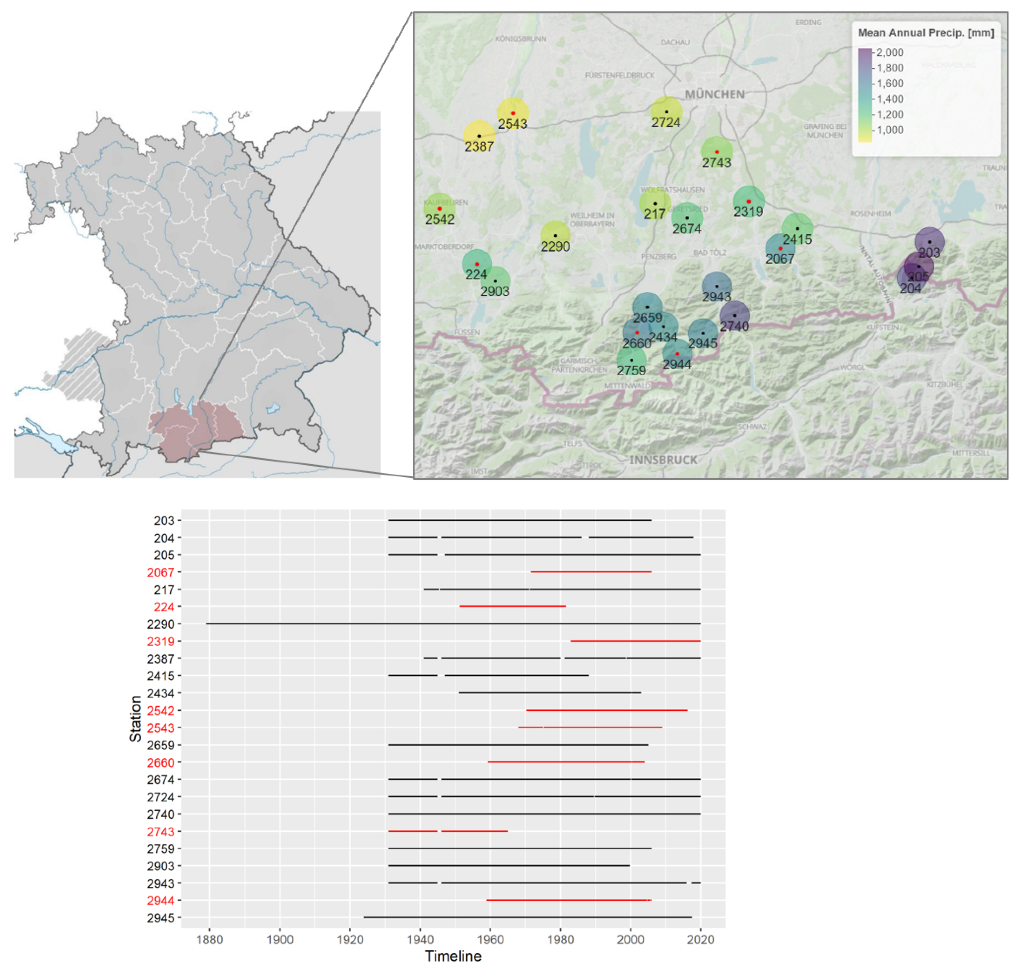
Figure 2.
Schematic illustration of the EVA approach followed in this study.
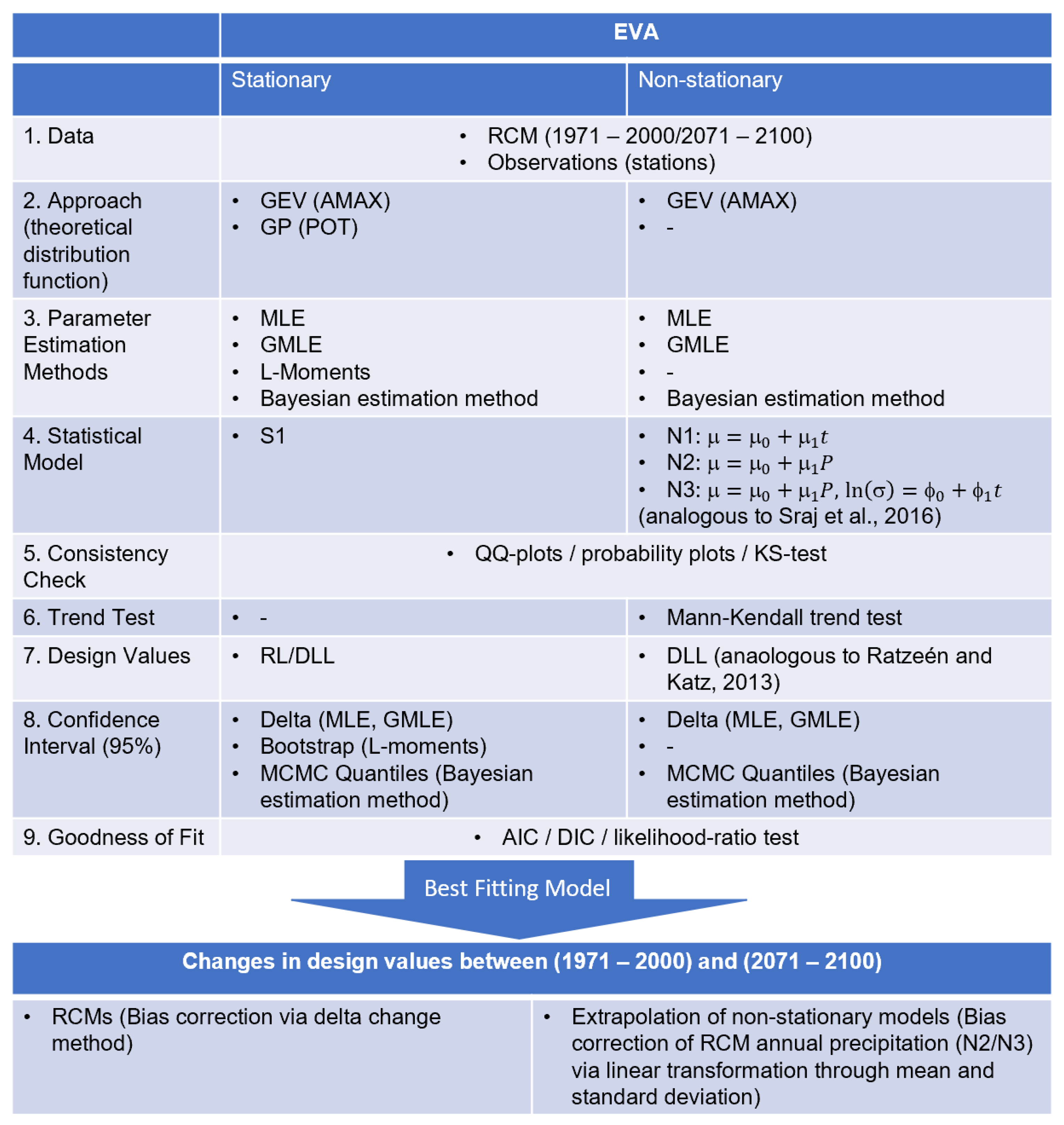
Figure 3.
100-year Return Level (RL) for all stations with all available parameter estimation methods (PEM) and for both approaches. Error bars indicate the 95% confidence intervals. Stations with time series length are indicated in red.
Figure 3.
100-year Return Level (RL) for all stations with all available parameter estimation methods (PEM) and for both approaches. Error bars indicate the 95% confidence intervals. Stations with time series length are indicated in red.
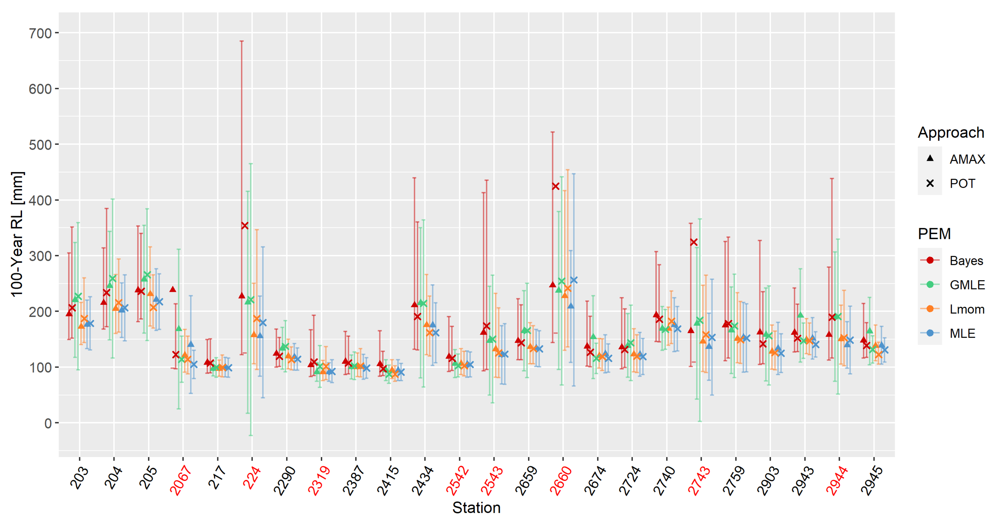
Figure 4.
10-year Return Level (RL) for all stations with all available parameter estimation methods (PEM) and for both approaches. Error bars indicate the 95% confidence intervals. Again, stations with time series length are indicated in red.
Figure 4.
10-year Return Level (RL) for all stations with all available parameter estimation methods (PEM) and for both approaches. Error bars indicate the 95% confidence intervals. Again, stations with time series length are indicated in red.
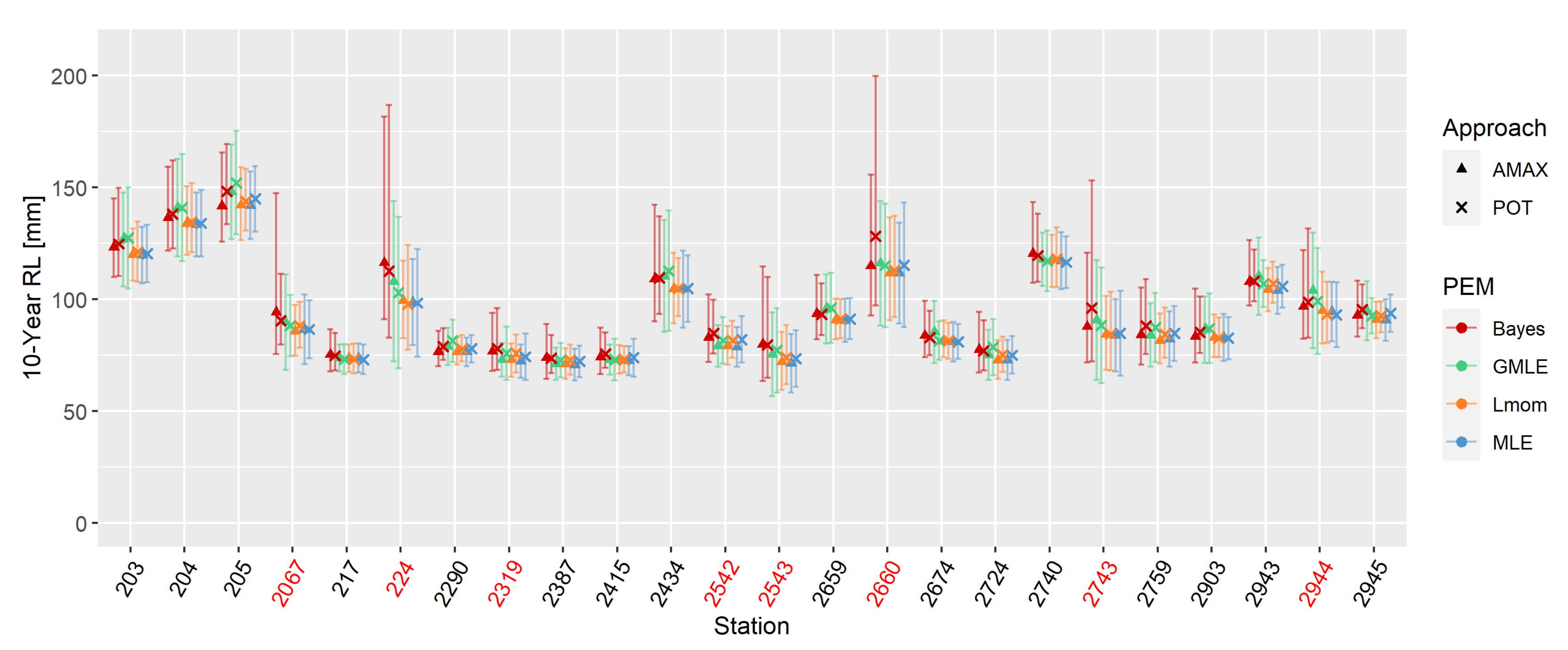
Figure 5.
Spatial representation of the 100-year RL for MLE (AMAX) (a), L-Moments (AMAX) (b), GMLE (AMAX) (c), and Bayesian estimation method (AMAX) (d). The circle size represents the uncertainty range between all PEM and the red dots indicate stations with time series lengths shorter than 50 years.

Figure 6.
Spatial representation of the 10-year RL for MLE (AMAX) (a), L-Moments (AMAX) (b), GMLE (AMAX) (c), and Bayesian estimation method (AMAX) (d): The circle size represents the uncertainty range between all PEM and the red dots indicate Stations with time series length shorter than 50 years.
Figure 6.
Spatial representation of the 10-year RL for MLE (AMAX) (a), L-Moments (AMAX) (b), GMLE (AMAX) (c), and Bayesian estimation method (AMAX) (d): The circle size represents the uncertainty range between all PEM and the red dots indicate Stations with time series length shorter than 50 years.
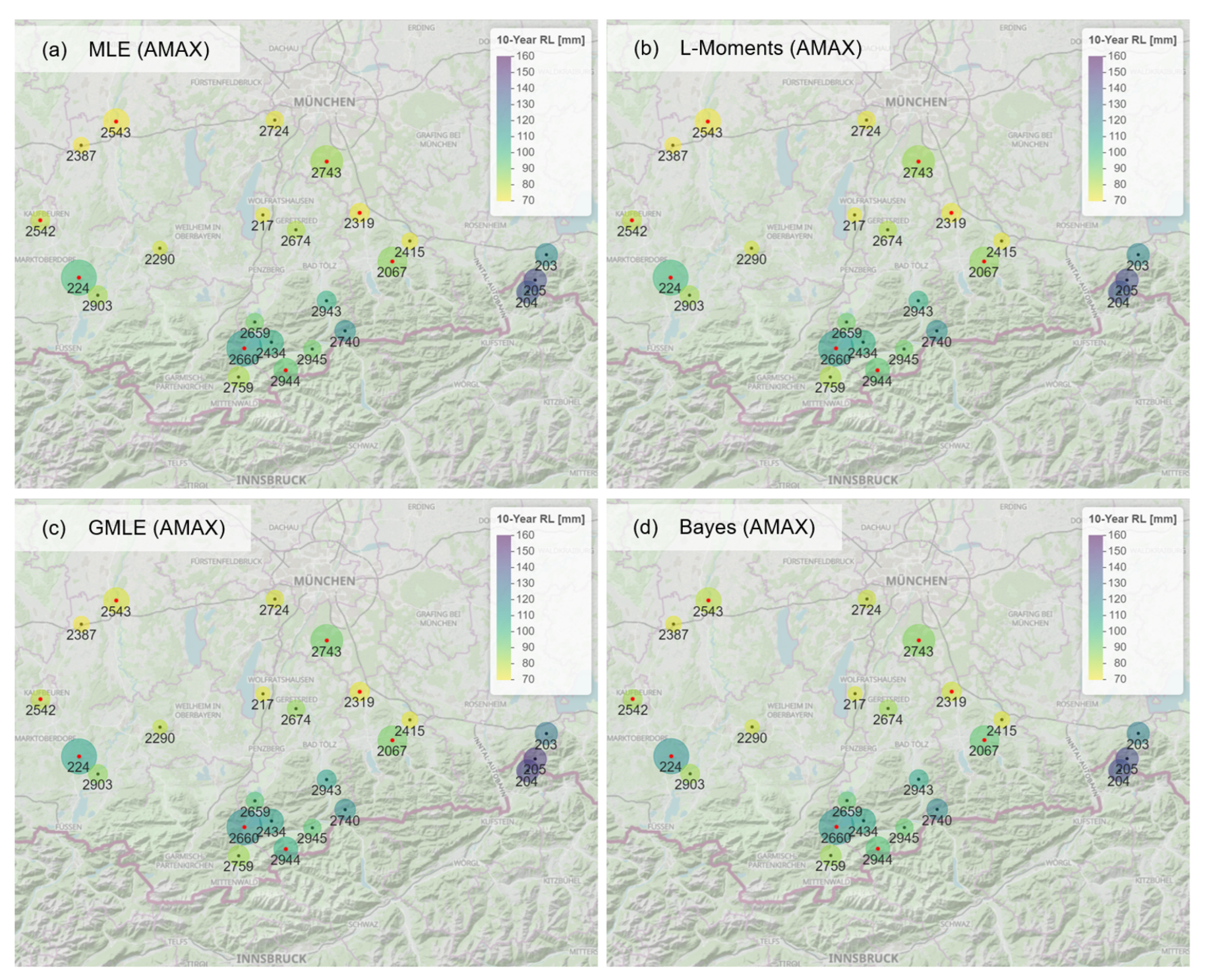
Figure 7.
Estimated slope for non-stationary location parameter and non-stationary scale parameter for the three-parameter estimation methods (MLE, GMLE, Bayes) and three non-stationary models (N1: , N2: , N3: and ).
Figure 7.
Estimated slope for non-stationary location parameter and non-stationary scale parameter for the three-parameter estimation methods (MLE, GMLE, Bayes) and three non-stationary models (N1: , N2: , N3: and ).
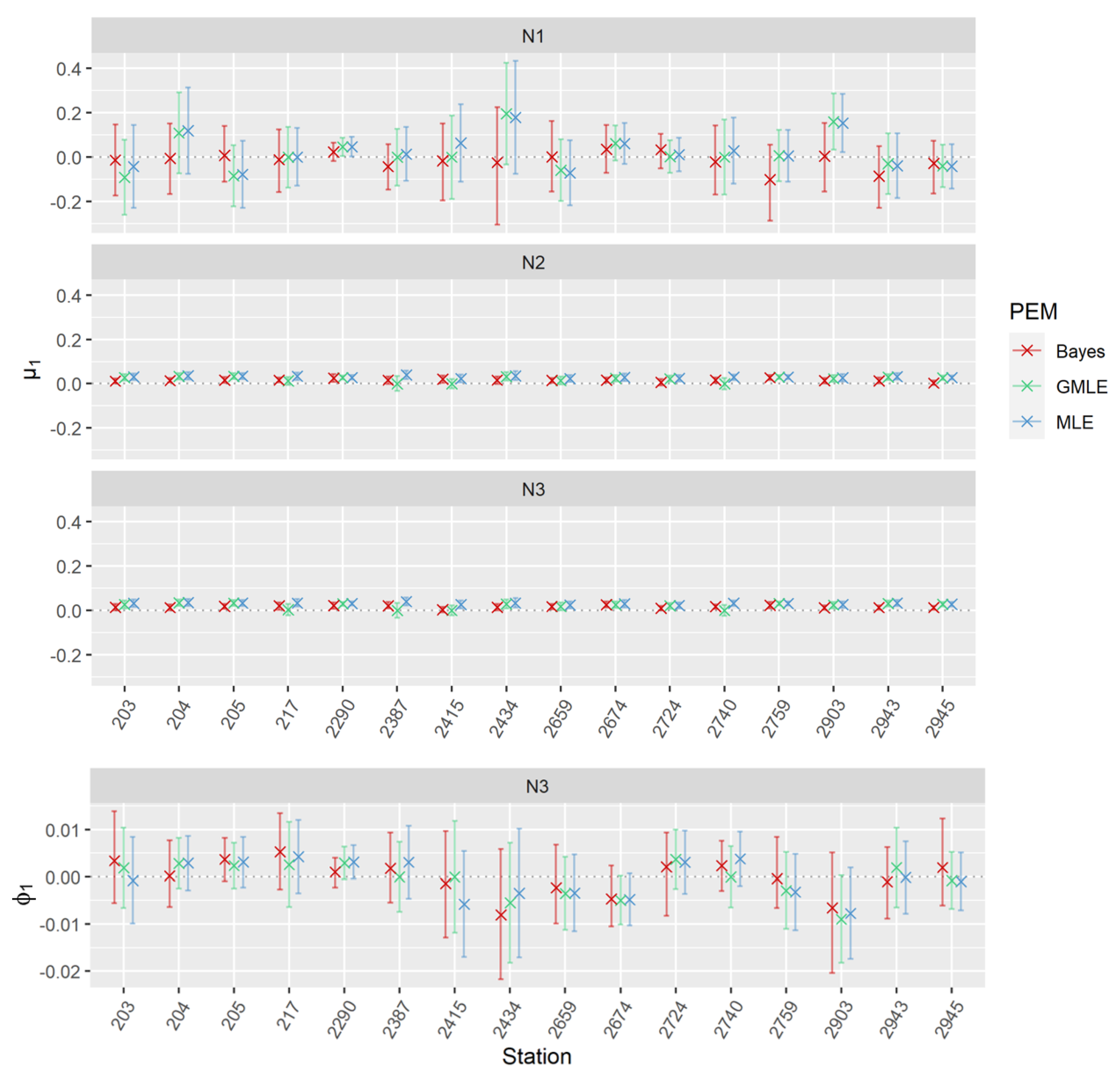
Figure 8.
100-year and 10-year obtained from extrapolated statistical models (2071-2100) with parameter estimation method MLE.
Figure 8.
100-year and 10-year obtained from extrapolated statistical models (2071-2100) with parameter estimation method MLE.
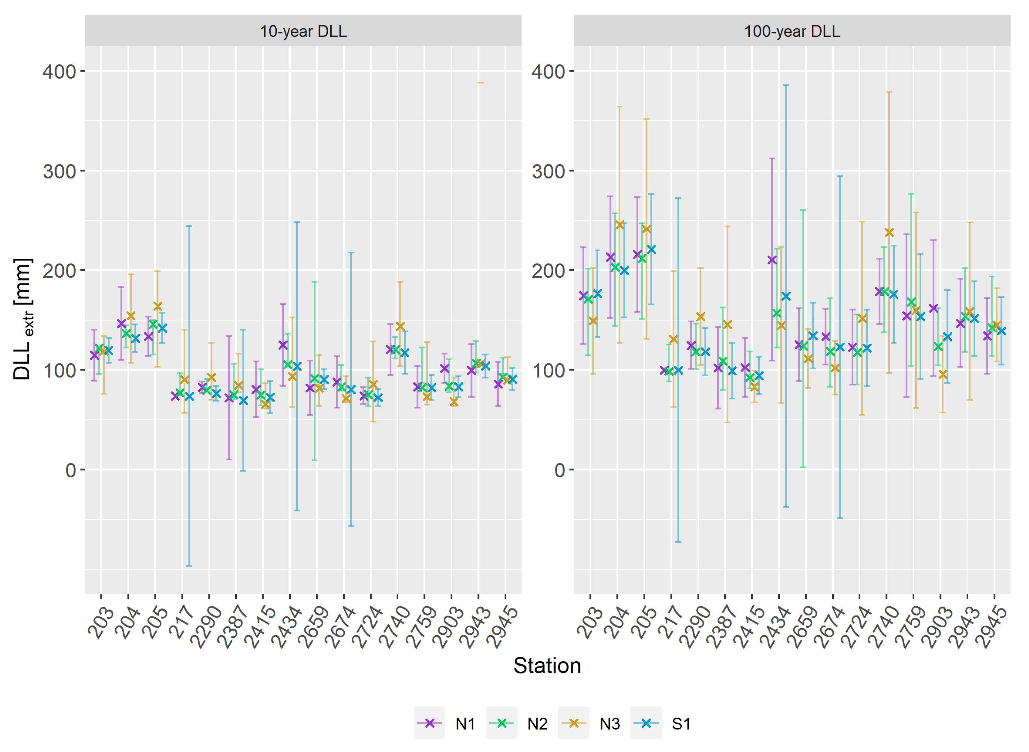
Figure 9.
Differences between 100-year design levels from historical RCM simulations and 100-year design levels from observations with indication of the range with approximately 10% deviation in green.
Figure 9.
Differences between 100-year design levels from historical RCM simulations and 100-year design levels from observations with indication of the range with approximately 10% deviation in green.
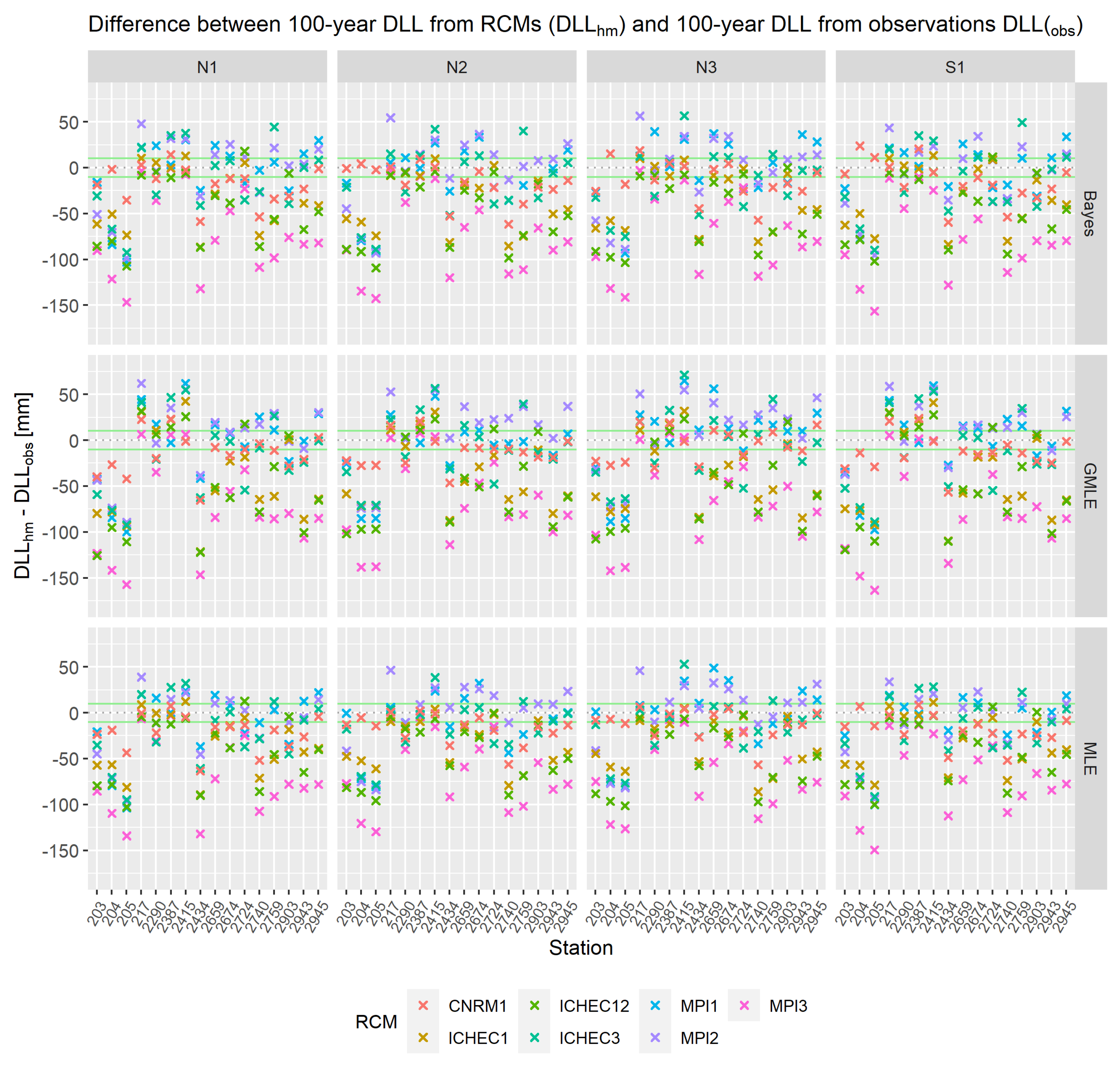
Figure 10.
Differences between 10-year design levels from historical RCM simulations and 10-year design levels from observations with indication of the range with approximately 10% deviation in green.
Figure 10.
Differences between 10-year design levels from historical RCM simulations and 10-year design levels from observations with indication of the range with approximately 10% deviation in green.
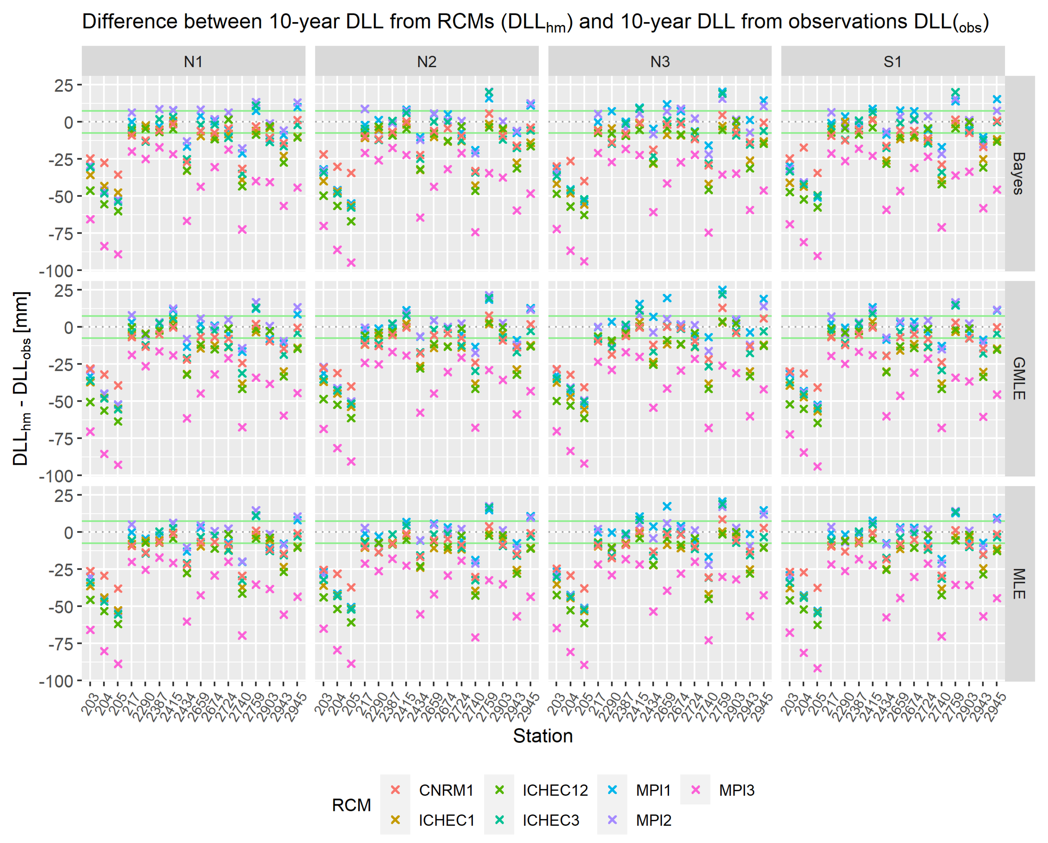
Figure 11.
Change in 100-year DLL between future (2071–2100) and historical climate (1971–2000) for delta change method and the extrapolation of statistical models S1 and N2.
Figure 11.
Change in 100-year DLL between future (2071–2100) and historical climate (1971–2000) for delta change method and the extrapolation of statistical models S1 and N2.
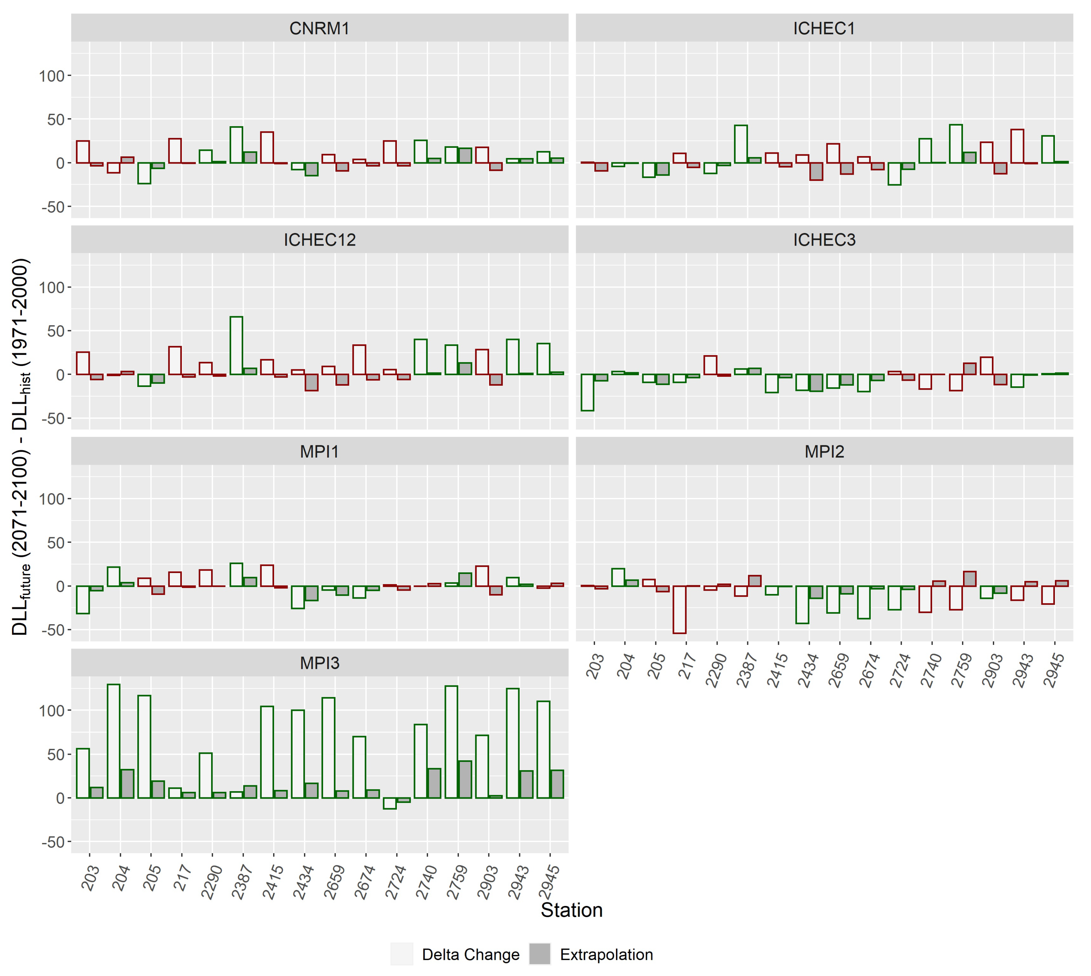
Figure 12.
Change in 10-year DLL between future (2071–2100) and historical climate (1971–2000) for delta change method and the extrapolation of statistical models S1 and N2.
Figure 12.
Change in 10-year DLL between future (2071–2100) and historical climate (1971–2000) for delta change method and the extrapolation of statistical models S1 and N2.
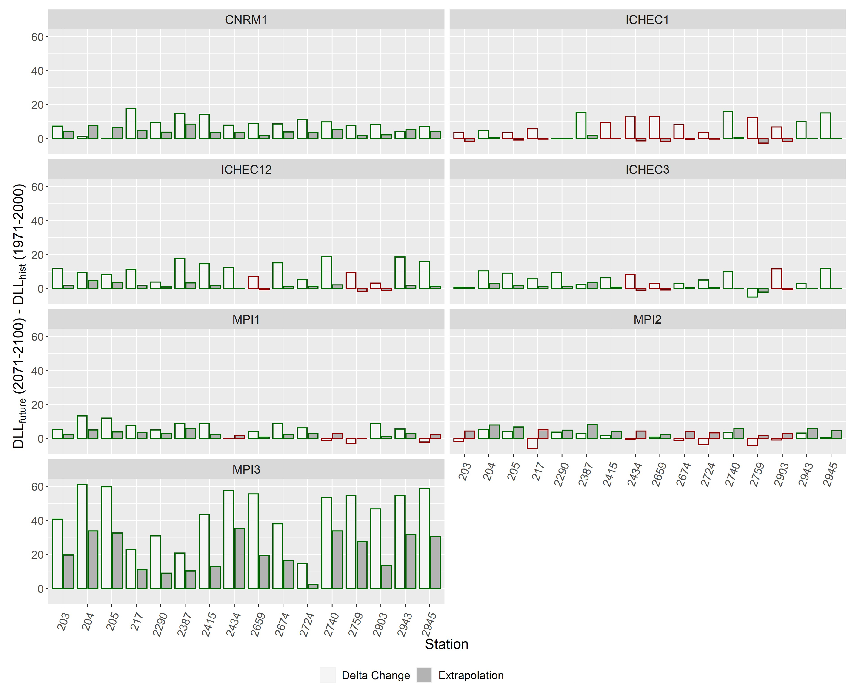

Table 1.
Overview of utilized GCM-RCM combinations from EURO-CORDEX.
| Driving Model (GCM) | RCM | Ensemble | ||
|---|---|---|---|---|
| ICHEC-EC-Earth | COSMO-crCLIM-v1-1 | r1i1p1 | 1950-2005 | 2006-2100 |
| ICHEC-EC-Earth | COSMO-crCLIM-v1-1 | r3i1p1 | 1950-2005 | 2006-2100 |
| ICHEC-EC-Earth | COSMO-crCLIM-v1-1 | r12i1p1 | 1950-2005 | 2006-2100 |
| MPI-M-MPI-ESM-LR | COSMO-crCLIM-v1-1 | r1i1p1 | 1949-2005 | 2006-2100 |
| MPI-M-MPI-ESM-LR | COSMO-crCLIM-v1-1 | r2i1p1 | 1949-2005 | 2006-2100 |
| MPI-M-MPI-ESM-LR | COSMO-crCLIM-v1-1 | r3i1p1 | 1949-2005 | 2006-2100 |
| CNRM-CERFACES-CNRM-CM5 | COSMO-crCLIM-v1-1 | r1i1p1 | 1951-2005 | 2006-2100 |
Disclaimer/Publisher’s Note: The statements, opinions and data contained in all publications are solely those of the individual author(s) and contributor(s) and not of MDPI and/or the editor(s). MDPI and/or the editor(s) disclaim responsibility for any injury to people or property resulting from any ideas, methods, instructions or products referred to in the content. |
© 2023 by the authors. Licensee MDPI, Basel, Switzerland. This article is an open access article distributed under the terms and conditions of the Creative Commons Attribution (CC BY) license (http://creativecommons.org/licenses/by/4.0/).
Copyright: This open access article is published under a Creative Commons CC BY 4.0 license, which permit the free download, distribution, and reuse, provided that the author and preprint are cited in any reuse.


