Preprint
Article

Large Eddy Simulation of Utility-Scale Wind Farm Sited over Complex Terrain

Altmetrics

Downloads

152

Views

188

Comments

0

A peer-reviewed article of this preprint also exists.

Jagdeep Singh  *,‡
,
Jahrul Alam  ‡

  ‡ These authors contributed equally to the work.

This version is not peer-reviewed

Submitted:

09 July 2023

Posted:

11 July 2023

You are already at the latest version

Alerts
Abstract
Wind energy is a rapidly expanding renewable energy technique. Wind farm developers need to understand the interaction between wind farms and the atmospheric flow over complex terrain. Large-eddy simulations provide valuable data for gaining further insight into the impact of rough topography on wind-farm performance. In this research, we investigate the influence of spatial heterogeneity on wind turbine performance. We conducted numerical simulations of a 12×5 wind-turbine array on various rough topographies. First, we evaluated our LES method through mesh convergence analysis, using mean vertical profiles, vertical friction velocity, and resolved and subgrid-scale kinetic energy. Next, we analyze the effects of surface roughness and dispersive stresses on the performance of fully developed large wind farms. Our results demonstrate that the ground roughness element’s flow resistance boosts large wind-farm power production by almost 68% in fully aerodynamic rough surface compared to flat terrain. Dispersive stress analysis revealed that the primary degree of spatial heterogeneity in the wind farm is in the streamwise direction, which is the “wake-occupied” region, and the relative contribution of dispersive shear stress is almost 45% to the overall drag. We also observed that the power performance of the wind farm in complex terrain outperforms the drag. Our study has implications for improving the design of wind turbines and wind farms in complex terrain to increase their efficiency and energy output.
Keywords: 
Subject: Physical Sciences  -   Fluids and Plasmas Physics

1. Introduction

Large wind farms are growing globally to reduce the energy-related carbon footprint [1,2,3,4]. Optimal onshore locations near coastlines in heavily populated regions are often not allowed for wind farm installation [5]. The other onshore sites are in rural areas, where the meteorological effects of forests and mountains can influence the local wind [6,7,8,9]. For large wind farms in rural onshore locations, the secondary circulation associated with the land-atmosphere interaction contributes to large-scale effects in wind farm layout optimization [1,10,11]. Computational analysis of characterizing the wind and atmospheric turbulence is relatively effective because measurements over the entire site are time-consuming. Creating a complete map of the local topography of the whole wind farm is affordable with modern high-performance computing facilities. However, as detailed in several recent articles [12,13,14,15,16], the fine grid causes a computational burden and becomes highly skewed if we resolve a steep mountain, which also deteriorates the numerical error.
This article employs a computational model of the local topography and the surface roughness to simulate the effect of complex terrain. Bhuiyan and Alam [16] demonstrates a scale-adaptive large eddy simulation (LES) method to simulate the land-atmosphere exchange of complex terrain. The LES of a wind farm in complex terrain can partially resolve the turbulence kinetic energy (TKE) and the Earth’s surface topography, and the subgrid model minimizes the effects of unresolved TKE and other meteorological phenomena [3,13,16,17]. Due to wake interactions and significant variability of ground elevations, the attached eddy hypothesis may not be accurate. Thus, it can enhance the dispersive stresses of the secondary motion close to the ground. The yawed flow is the horizontal misalignment of an incoming flow to the rotor axis. Studies have shown that in wind farms, neglecting the land-atmosphere exchange, yawed flow can reduce power production and increase the load and moments at the rotor blade [1,4,18,19].
This article considers a scale-adaptive LES method to account for the land-atmosphere exchange and focuses on the effects of airflow reduction by complex terrain and forests [20]. To gain a better insight into the effects of spatial inhomogeneity of the Earth’s surface, we follow the method proposed by Bao et al. [21] and incorporate the local stress of complex terrain into the momentum equation by adapting resolved stresses at grid points adjacent to the Earth’s surface. We call this approach the ‘near-surface model’, which differs from the classical wall models by the way it formulates velocity and stress conditions on the complex terrain [22,23,24,25]. Chow et al. [26] reviewed the existing scale-adaptive LES of atmospheric boundary layer flows (see also [27,28,29]). Among them are blending the characteristic length scales [28], hybrid RANS-LES in the near-surface region [27], and the canopy stress model [29]. In the current development, we employ Helmholtz’s second vortex theorem and the vortex stretching mechanism to capture the transition of characteristic scales from one flow regime to the other, such as convergence zone, pure shear, or inflection, to dynamically adjust the dissipation rate [16,17,30,31]. We model wind turbines as actuator disks, leading to a drag source in the atmospheric boundary layer [1,4,19]. Readers interested in the scale-adaptive LES method and the actuator disk model may consult the cited reference.

1.1. Surface roughness

Wind turbines extract energy at heights between 30 m and 150 m and contribute toward the dissipation of energy by surface roughness. The atmospheric sciences community has thoroughly examined the effect of surface roughness caused by mountains, forests, vegetation, etc. Surface roughness is generally represented through the aerodynamic roughness length ( z 0 ) and the Monin-Obukhov similarity theory [32,33]. The impact of an isolated hill on the turbine performance depends on the turbine size and its position relative to the mountain [6,8]. Some studies show wind farm performance can be enhanced over hilly terrain [6,8]. However, other studies have observed that overall surface drag may outweigh the benefit of the local speed-up effect resulting from the disturbances of the surface protrusion (e.g., [11] and the refs in [17]). Past studies of wind farms in complex terrain [5] have either empirically tuned the earth-atmosphere exchange [34,35,36] or ignored it [1].
Wind tunnel experiments verified that the laminar-turbulent transition occurs in the boundary layer due to the surface-mounted roughness elements [34,35,37,38,39]. Cao et al. [40] studied the effects of 2D hills on the turbulent boundary layer. Ye et al. [36] investigated the impact of various roughness elements on flow resistance in mountainous regions. The surface drag and turbulent momentum transport caused by surface roughness primarily constrain the near-surface mean wind speed, dissipate a fraction of the kinetic energy, and alter the atmospheric boundary layer profile [36,40,41,42]. The representation of subgrid-scale effects of mountains within a scale-adaptive LES of atmospheric boundary layer has improved in recent years [15,16,21]
An isolated hill with a smooth surface exerts a blockage effect on the downstream side, which may reduce the power output and enhances the fatigue load on relatively small turbines [6]. The power output of a wind turbine sited on top of a hill may be (about 82 % ) higher relative to that on a flat terrain. Vanderwende and Lundquist [2] observed that the power output of a wind farm over a vegetated land increases by 14% when the roughness length ( z 0 ) changed from 0.1 m to 0.25 m due to the increased crop height. Tobin et al. [43] observed that optimally placed artificial windbreaks may increase the power production by at least 10% [8,11,44]. In contrast, the overall power losses due to wake effects could be up to 20 % of the total power for wind farms over a flat terrain [45].
Each turbine also poses an additional drag and increases near-surface kinetic energy dissipation [20,46]. Therefore, sustaining the high power output of a large wind farm depends on whether another source of kinetic energy can compensate for the extra energy dissipation by a large array of turbines. For example, 3% variations of the hub height velocity caused by a complex terrain could lead to approximately 27% fluctuations in the power output [5]. The irregular topography of complex terrain, such as the Rocky Mountains and Tibetan Plateau, coastlines, or varying land use are efficient for the vertical kinetic energy transfer from aloft, and thus, can play an essential role in wind farm optimization [2,16,46,47].

1.2. Form-induced dispersive stress

Complex terrain acts as a large-scale obstruction to the flow, creating dispersive stress, of which the subgrid scale effects are essential in scale-adaptive LES of wind farms. Past studies have addressed drag reduction, empirical formulations of roughness effects in the secondary turbulent motions due to rough walls [48], forests, canopies, vegetation, coral reefs, etc. [49], and arrays of wind turbines [10,47]. The double-averaging method, introduced by Raupach and Shaw [50] for canopy turbulence [51] provides the dispersive stress of turbulent flow over wind turbines [10]. For dense canopies, the form-induced drag could significantly affect the lower canopy layer [52]. Poggi et al. [53] suggest dispersive stresses could reach up to 30% of the Reynolds stresses [49,54]. Moltchanov and Shavit [49] observed that the normal dispersive stresses are relatively more sensitive to the wake than the recirculation zone. The dispersive stress can originate from the vorticity generated by surface irregularities [55]. In the wind tunnel experiment of urban-like roughness elements, Cheng and Castro [56] observed that dispersive stresses are negligible compared to Reynolds stresses. In turbulent flow over an array of cubes, Santiago et al. [57] observed that Reynolds and dispersive stresses contribute equally [58,59]. However, recent studies suggest dispersive stresses account for 30% to 40% of the Reynolds stresses [60,61].
For wind farms in complex terrain, the secondary motion of the sparse canopy formed by wind turbines leads to enhanced dispersive stresses (e.g. [50]). However, it remains unclear whether a greater downward transport of kinetic energy may be sustained when dispersive stresses are due to the simultaneous effects of terrain complexity and wind turbines. In particular, no estimate for a sustained rate of the downward transport of kinetic energy is available, which may compensate the loss within large wind farms. This work provides the contributions of the dispersive, and Reynolds stresses to the total drag generated by wind farms in complex terrain.

1.3. Outline

This article considers a scale-adaptive LES of a wind farm consisting of 12 × 5 turbines (with a rotor diameter of 100 m) sited over a complex terrain. Instead of explicitly resolving the terrain roughness elements, we employ the geostrophic drag law within a near-surface model to simulate the effects of the terrain. We set the vertical inflow profile of the streamwise velocity with a fixed wind speed at the hub height and employ a stochastic forcing method to inject turbulence intensity into the spanwise and wall-normal components of the inflow velocity. This approach does not recirculate nonlinear eddy dynamics on embedded inflow domains.
We assess the resolution requirements for utility-scale wind farm simulations considering standard criteria. We evaluate the influence of spatial heterogeneity and drag coefficient on the performance of wind farms. Based on the utility-scale wind farm flow fields over complex terrain, we assess the relative contributions of the dispersive and Reynolds stress to the total drag in wind farms. Then, we compare the effects of spatial heterogeneity on the atmospheric turbulence around wind farms. Here, we show that the power production of a wind farm in complex terrain outweighs the associated drag of the roughness elements. Finally, we report the relative contribution of dispersive stresses to the overall drag, where dispersive stresses are due to both the roughness elements and the turbines.
The article is organized as follows, First, Section 2 provides the mathematical description of numerical methods and the theory and implementation of the near-surface model used for the present study. Section 3 presents the validation and the analysis of the result. Finally, Section 4 summarizes the main results indicating potential future research directions.

2. Numerical Methods

2.1. Large eddy simulation (LES)

This study employs an in-house LES code [16,31,62] to simulate the high Reynolds number neutral atmospheric boundary layer flow over an array of wind turbines. The LES method solves the filtered continuity equation
u ˜ i x i = 0 ,
and the momentum equations
u ˜ i t + u j ˜ u ˜ i x j = p ˜ x i τ i j x j + f i χ ( x , t ) ,
where u ˜ i ( x , t ) denotes the spatially filtered velocity characterized by a length scale of Δ les = 2 Δ x Δ y Δ z 3 . The subscripts i = 1 , 2 , 3 represent streamwise, spanwise and surface-normal directions, respectively.
In Eq 2, a subgrid model should correctly represent the second last term so that τ i j S i j ¯ accounts for the production of small-scale turbulence kinetic energy, where ( · ) ¯ represents the ensemble average, S i j = ( 1 / 2 ) ( u i / x j + u j / x i ) , and τ i j = u i u ˜ j u ˜ i u ˜ j . Borue and Orszag [63] indicate that a model of the subgrid stress τ i j would account for the energy cascade through the process of vortex stretching. Several recent investigations have clearly outlined the role of vortex stretching and strain self-amplication to formulate a cornerstone principle for the energy cascade in LES [30,64]. In this article, we have considered the scale-adaptive LES model [31] to represent the residual stress tensor τ i j . The scale-adaptive LES is based on the idea of energy cascade by vortex stretching [16,31], and its extension to wind farm simulation is detailed by Alam [17].

2.2. Near-surface model

Close to the Earth’s surface, resolving the energy-containing eddies with an isotropic grid is very costly [29], and an LES of the atmospheric boundary layer typically uses finer grid spacing in the vertical direction than in the horizontal [21,65]. Atmospheric LES codes treat horizontal and vertical dissipation separately, often using a damping function to adjust the eddy viscosity [15,66]. Such LES method also utilizes the conventional Monin-Obukhov similarity theory to model the effects of viscous layer.
For wind farms in complex terrain, Monin–Obukhov similarity-based boundary conditions are not appropriate if the lowest grid level is located well within the roughness sublayer [67]. The Monin-Obukhov similarity theory states that the vertical distribution of the wind shear is u ¯ / z u * / ( k z ) , which leads to the wind profile
u ¯ ( z ) = u * k ln z z 0 ,
where z 0 is the constant of integration and is known as the aerodynamic roughness length and u * is the characteristic velocity scale, also known as friction velocity. Thus, in the atmospheric boundary layer [15,22], a parametrization of the horizontal components of the turbulent stresses at z = 0 is
τ i 3 = c f ( u ¯ 1 2 + u ¯ 2 2 ) 1 / 2 u ¯ i , i = 1 , 2 ,
where the frictional coefficient c f is diagnosed from the velocity u ( z 1 ) given by Eq 3 at z = z 1 [15,21,32], and more specifically, one would not set z 1 < z * [67]. Here, z * is the height of the roughness layer.
The upper limit of the roughness sublayer ( z * / z 0 ) varies approximately between 10 and 150. Thus, for z * / z 0 = 100 with z 0 = 1 m (e.g. for forests), the depth of the roughness sublayer ( z * ) may be up to 100 m. The specification of ground shear stress via Eq 3 is not consistent with boundary layer scaling laws if Δ z < 100 m for wind farms in forested complex terrain.
An assumption of LES is that the subgrid-scale dissipation accounts for the subgrid-scale turbulence production [68,69]. The exact viscous dissipation 2 ν S ij S ij (note the bold face) must be equal to the sum of filtered energy flux Π = τ i j S i j and resolved viscous dissipation 2 ν S i j S i j such that [70]
Π 2 ν S i j S i j = 2 ν S ij S ij .
A classical subgrid model based on the filtered strain rate, yielding
Π ( x , t ) = c s ( x , t ) Δ les 2 ( 2 S i j S i j ) 3 / 2
violates the local isotropy hypothesis in LES of wind farms. The filtered energy flux Π will not vanish when all the scales are resolved in a wind farm [70]. Within the roughness sublayer [66], we can modify the eddy viscosity ν τ ( x , t ) to account for the roughness effects into the filtered energy equation while evaluating Eq 3 at z = z 1 to provide boundary conditions. Consider the subgrid scale stress averaged over a horizontal plane in the following form [66]
τ i 3 2 [ γ ( z ) ν τ + ν T ] u i z , i = 1 , 2 ,
where γ ( z ) is the damping factor that accounts for the shear-driven nature of the near-surface dynamics [29] and ν T is the mean-field eddy viscosity needed to force the vertical velocity gradient to match with that from the similarity theory at z = z 1 [66]. The mean-field eddy viscosity model accounts for the Gabor-Heisenberg uncertainty, where the subgrid model is local in physical space and nonlocal in wave number space.
In scale-adaptive LES, we assume that i) vortex stretching drives the energy cascade and maintains the Kolmogorov energy spectrum, and ii) that turbulence production, kinetic energy cascade, and viscous dissipation are in local equilibrium [16,17]. Thus, we can relax the horizontal averaging in the mean-field eddy viscosity model proposed by Sullivan et al. [66], and consider that
[ τ 13 2 + τ 23 2 ] 1 / 4 = C D 1 / 2 u ( x , y , z 1 ) ,
where the drag coefficient is
C D = k / ln ( z / z 0 ) ψ M ( ξ ) 2
and for neutral atmospheric boundary layer flow ψ M ( ξ ) = 0 . Combining Eq 3 with Eq 4 we estimate τ i 3 ( x , y , z 1 ) for i = 1 , 2 , and finally, we estimate the mean-field eddy viscosity ν T from
τ i 3 = 2 [ ν τ ( x , y , z 1 ) + ν T ] u i z , i = 1 , 2
In the above discussion, we follow Sullivan et al. [66] and Basu and Lacser [67] to account for the near-surface effects into the scale-adaptive LES method employed in this work. Recent studies, such as [16,71], have considered a similar formulation in LES of the atmospheric boundary layer flow over hilly terrain.

3. Results, and Discussions

The following analysis studies the interaction between a wind farm and complex terrain. We do not explicitly resolve irregular topography, such as mountains, coastlines, or urban variations in land use. Wind energy applications usually characterize complex terrain by the roughness class associated with a roughness length scale. This work focuses on wind farms’ flow structure and performance, considering each wind turbine as a Gaussian actuator disk [72]. First, we discuss the effect of grid resolution on ABL profiles, wake profiles, turbulence, and wind farm performance. Second, we investigate the effect of surface roughness on the performance of wind farms. We investigate various factors contributing to the increased power production in wind farms. Third, we examine the relative contribution of dispersive stresses and Reynolds stress for wind farms in complex terrain.

3.1. Simulation setup

This work simulates a 12 × 5 array of wind turbines in the neutrally stratified atmospheric boundary layer over a complex terrain. Each turbine has a hub height of 100 m and a rotor diameter of D = 100 m. Turbines are separated by a distance of S x = 7 D in the x-direction and S y = 5 D in the y-direction. The wind farm is schematically shown in Figure 1. The presence of the wind turbine array affects the upwind flow conditions known as blockage effect [73,74]. Strickland and Stevens [75] observed that the induction region is more apparent and may affect up to 13D on upwind flow conditions if the interspacing between the wind turbine is relatively less. Therefore, we kept the first row at a distance of 14D downstream of the inlet boundary at x = 0 . At the inlet boundary, x = 0 , the streamwise component of the velocity was assigned to U ( z ) = ( u * / k ) ln ( z / z 0 ) , where u * is chosen according to a desired Reynolds number ( R e = 6.7 × 10 7 ) based on the undisturbed velocity at hub height. We have the initial condition u ¯ i ( x , 0 ) = U ( z ) , 0 , 0 . A stochastic forcing is considered at the inlet boundary x = 0 to provide transient perturbations into the spanwise and surface-normal velocities, where U ( z ) , v ( 0 , y , z , t ) , w ( 0 , y , z , t ) is the boundary condition at x = 0 . To apply a stochastic force at x = 0 , we assume an ensemble of eddies with centers randomly distributed in space at n spot locations, while their axis of rotation is aligned in the x direction. Such eddies maintain an enhanced level of variance by extracting energy from the mean flow and passing it to the perturbation fields.
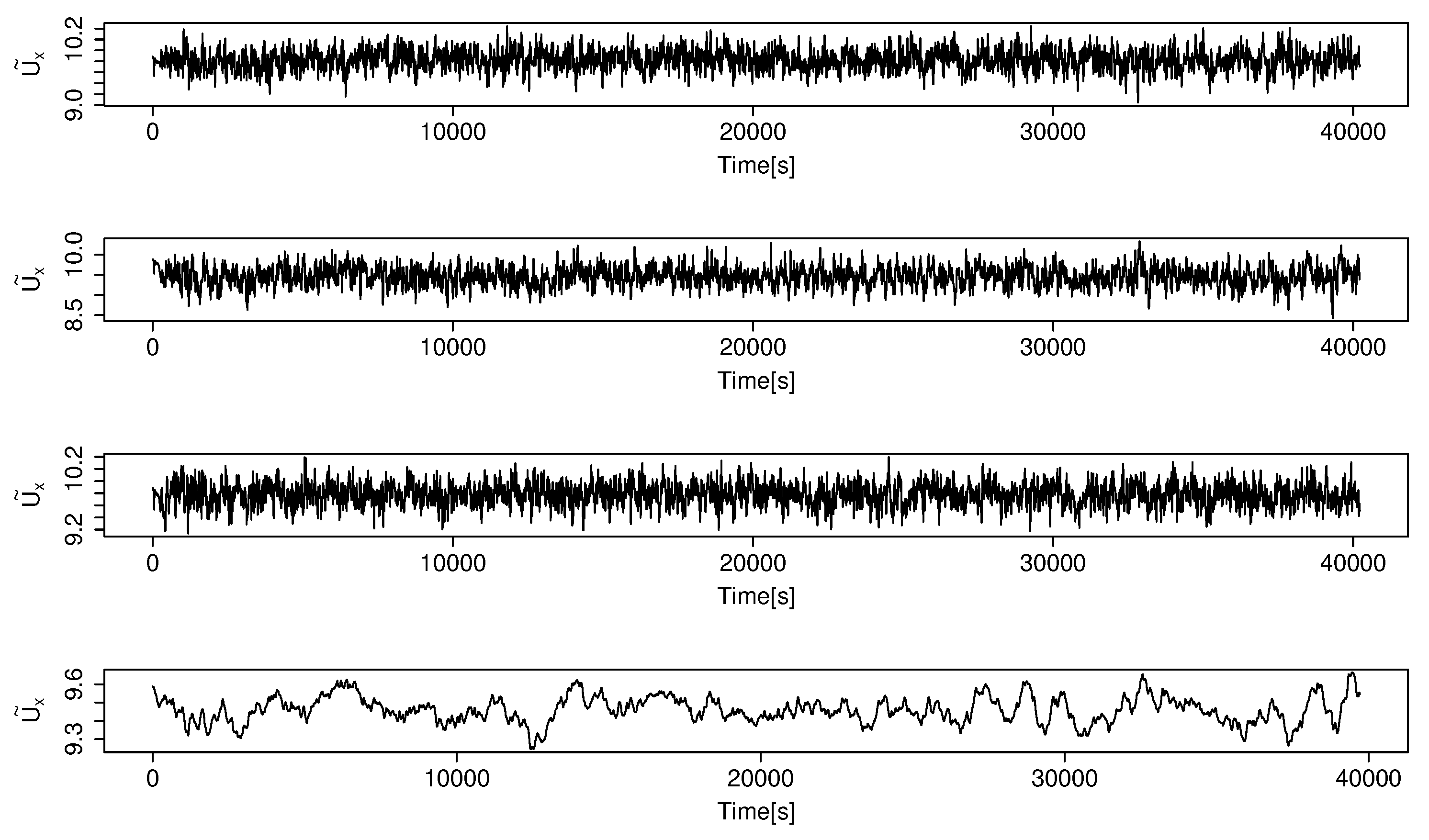
To illustrate the transitional flow development in scale-adaptive LES for z 0 = 1 m, we sampled the velocity time series at ( x , y , z ) = ( 12 D , y , 1 D ) in front of the center of three turbines denoted by T2, T3, and T4 in Figure 1. These three time series of velocity would represent the phenomena that atmospheric turbulence produces chaotic motions in the atmospheric boundary layer, which inhibit turbulence mixing. The streamwise component of each of the three velocity time series is shown in Figure 2. This result indicates that episodes of turbulent bursts persist in the streamwise velocity and pass through the first row of wind turbines. The outcome of applying the moving average with a window of 512 [s] into the streamwise velocity in front of turbine T2 is shown at the bottom plot of Figure 2.
In the following section, we like to understand the grid resolution and time step necessary to capture the wind turbine wakes.

3.2. Effect of mesh resolution

The present study considers a range of resolutions, including isotropic and non-isotropic refinements, to ensure that we had both poorly-resolved and well-resolved simulations. Following the criteria outlined by Pope [69], we discuss the effects of mesh resolution on the wake profiles, turbulence statistics, and the performance of a wind farm [65,76]. Table 1 summarizes 7 representative cases of LES for a mesh resolution study. The aerodynamic roughness length ( z 0 ) of the inlet wind profile was set to 1 m. In LES Eq 2, one assumes that u ˜ i ( x , t ) is a spatially filtered velocity. However, the numerical solution u ˜ i ( x , t ) of Eq 2 is, in principle, a resolved part of the filtered velocity [69]. Thus, to extract the statistics of the resolved velocity u ˜ i ( x , t ) , Pope [69] suggests to average the flow field within a time interval, which is 45 T * in the present study. The flow was sampled at a time step such that CFL = 1, where T * = D / u * is the large-eddy turnover time unit, and CFL stands for Courant–Friedrichs–Lewy condition.

3.2.1. Mean profiles and turbulence

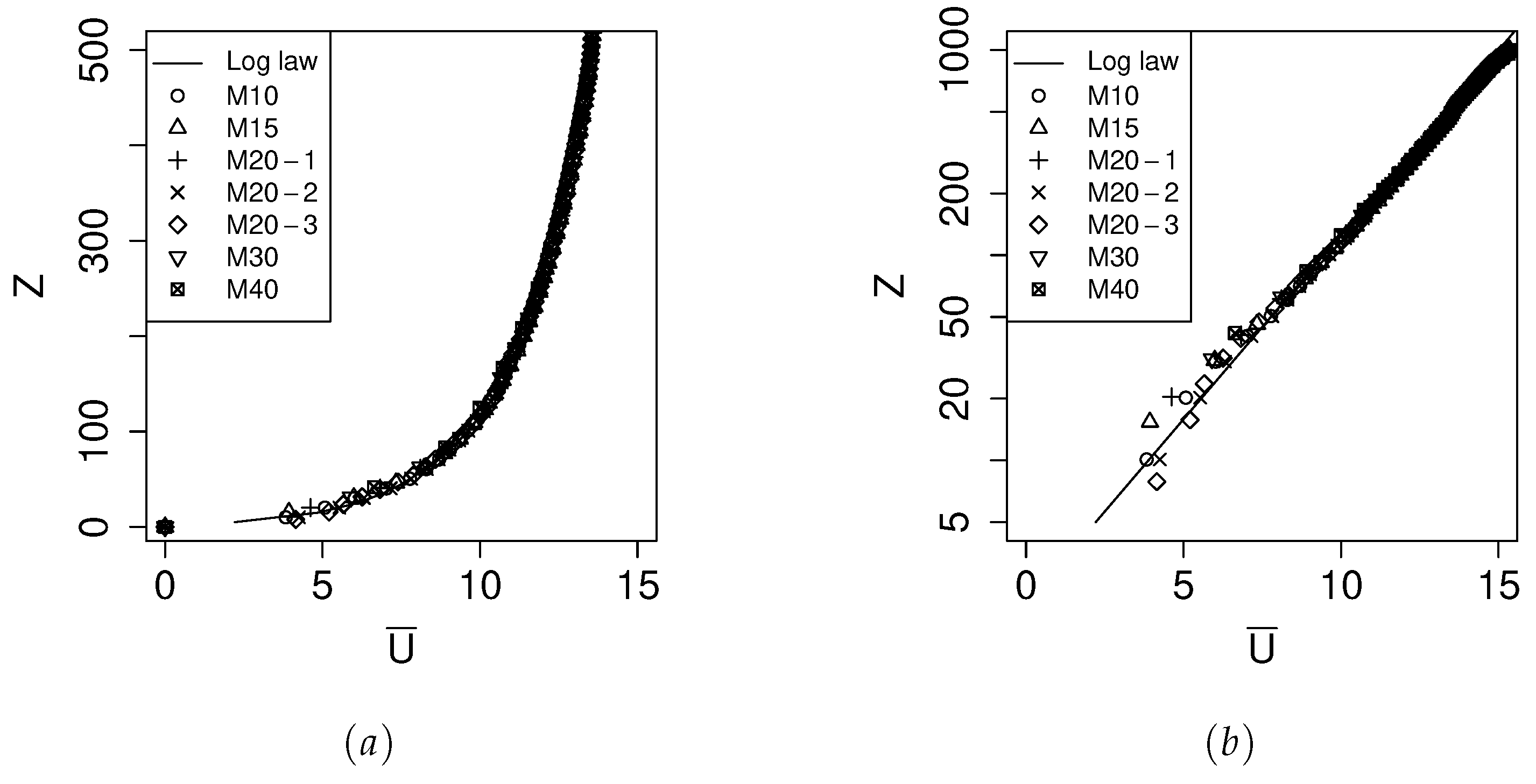
Figure 3 shows the vertical profile of the mean streamwise velocity on the vertical mid-plane at 2D upstream of the first row of the wind farm. The mean was obtained within a time interval of size 45 T * , and the result has been compared with the log-law wind profile given by Eq 3. The vertical profile of the mean streamwise velocity follows the logarithmic profile given by Eq 3 for all resolutions listed in Table 1. When the grid spacing is 40 m in all three directions, the atmospheric boundary layer flow is poorly-resolved [65]. Wurps et al. [65] suggests that a grid spacing of about 10 m is necessary for well-resolved LES so that the vertical profile of mean streamwise velocity is fully captured.
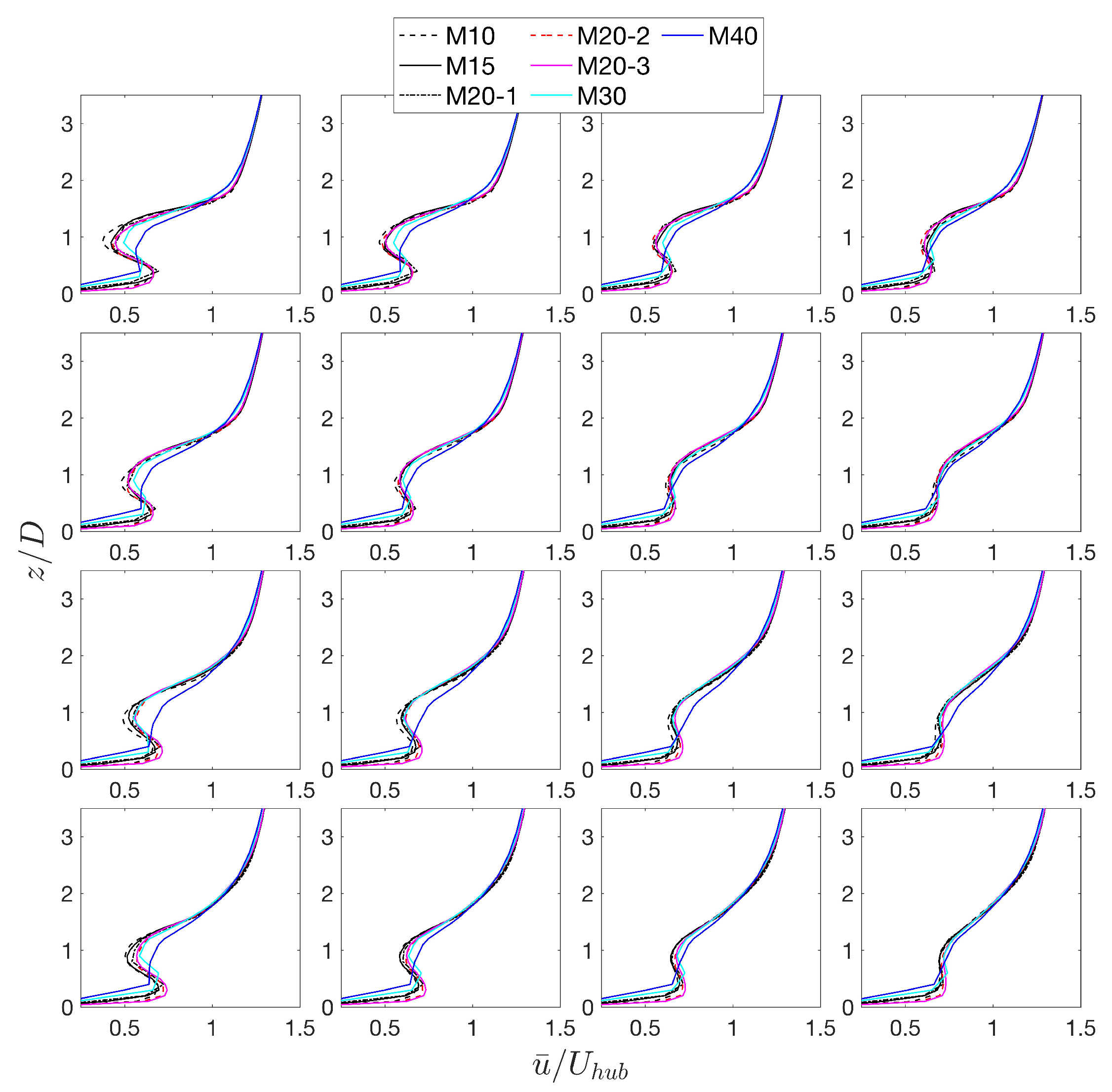
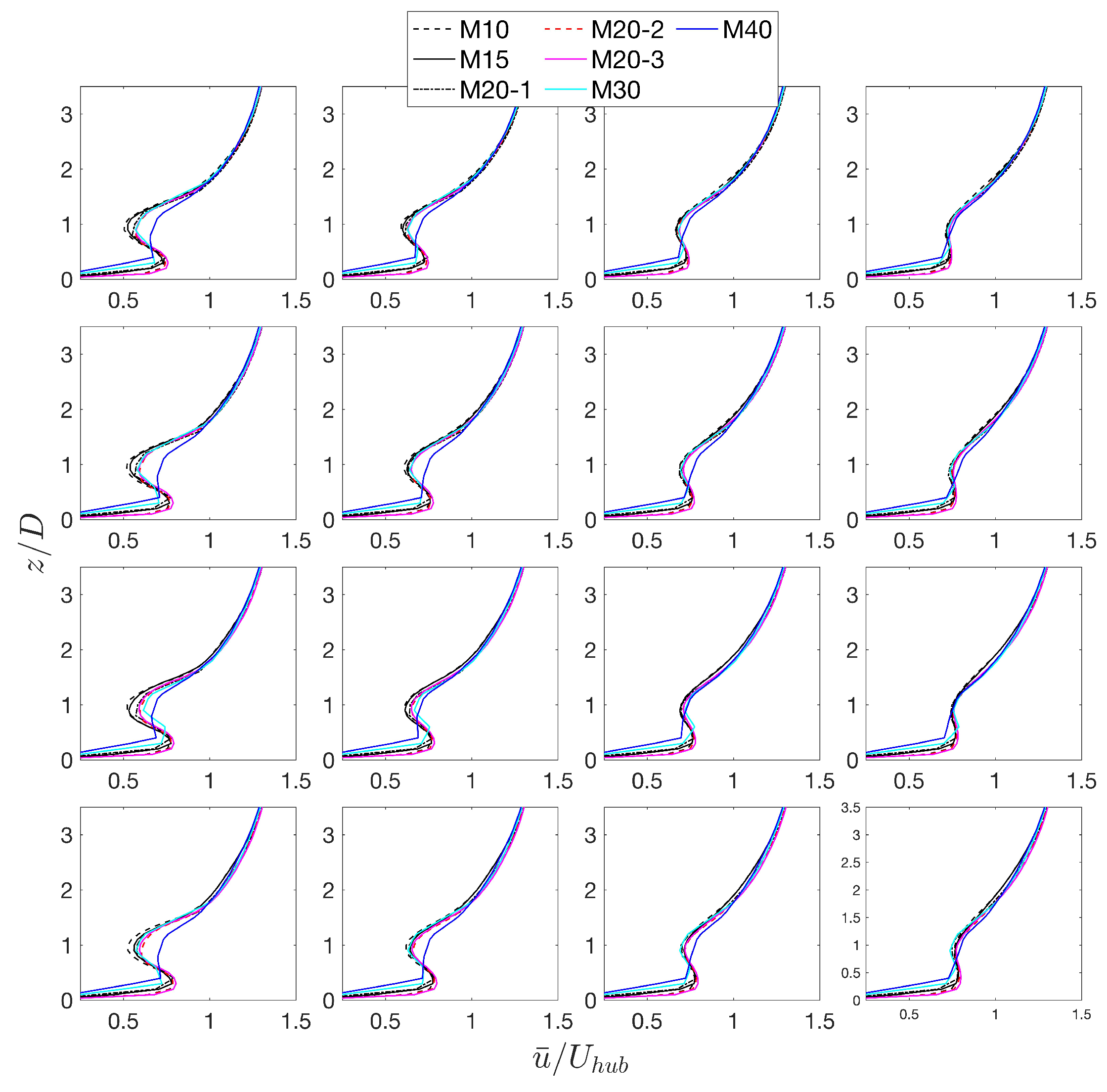
Figure 4 shows vertical profiles of the mean streamwise velocity on the vertical mid-plain at four wind turbine rows 1-4. We compare the profiles at locations 2D, 3D, 4D, and 5D behind the turbine for each row. Similarly, Figure 5 shows vertical profiles for rows 5, 7, 10, and 12. The plots in Figure 4 and Figure 5 compare the wake profiles among 7 resolutions. The results indicate that the solution converges to the wake profiles of case M10. The profiles of cases M30 and M40 show deviations from that of case M10. A grid spacing of 20 m in all directions is necessary to capture the wakes using the scale-adaptive LES.
Turbulence statistics of a wind farm provide insight into how kinetic energy is entrained from aloft. For this analysis, we consider the Reynolds decomposition
u ˜ i ( x , t ) = u ¯ i + u i ( x , t ) ,
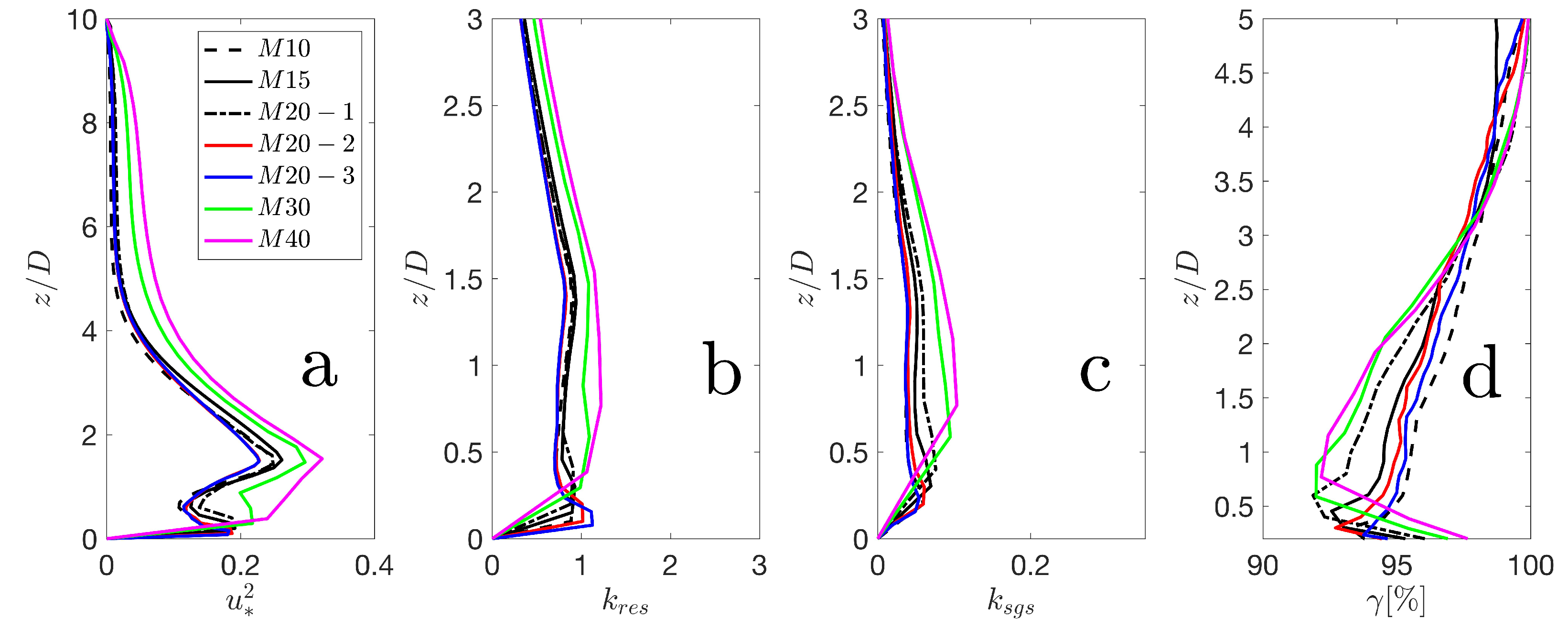
where u ˜ i ( x , t ) is the numerical solution of Eq 2 and u ¯ i is the ensemble average within a time interval of length 45 T * . The Reynolds stress resolved by the LES method is τ i j R = u i u j ¯ . The fraction of the turbulence kinetic energy modelled by the scale-adaptive LES method is k s g s = ( 1 / 2 ) τ i i , where the resolved turbulence kinetic energy is k r e s = ( 1 / 2 ) τ i i R . The ratio of resolved to the total turbulence kinetic energy is effective resolution γ = k r e s / ( k r e s + k s g s ) [68]. A value of γ = 0.8 indicates that the LES method has captured about 80% of the total turbulence energy. In this context, we have analyzed the shear stress u * 2 , resolved kinetic energy k r e s , subgrid-scale kinetic energy k s g s , and effective resolution γ .
Figure 6 shows vertical profiles of u * 2 , k r e s , k s g s , and γ , where u * 2 = u w ¯ 2 + v w ¯ 2 1 / 2 represents the shear stress. Vertical shear stress profiles exhibit negligible dependence on the grid resolution except for cases M 30 and M 40 , (see Figure 6a). Figure 6b shows that in most part of the boundary layer, the resolved TKE for coarser grid cases ( M 30 & M 40 ) were higher than that for finer grid cases. Wurps et al. [65] also noted a similar scenario in atmospheric boundary layer simulations without wind turbines. Celik et al. [77] observed that in wall-bounded flows, resolved strain S ¯ i j tends to be small, thereby resulting in relatively less resolved dissipation ϵ = 2 ν s g s S ¯ i j S ¯ i j , which leads to higher resolved TKE.
Figure 6d illustrates the ratio ( γ ) of the resolved TKE to the total TKE in the wind farm, which shows a clear dependence on the resolution. Notably, finer grids consistently exhibit larger γ values than coarser grids across the entire boundary layer. It is worth noting that as the vertical resolution increases, such as in cases M 20 -2 & M 20 -3, the value of γ approaches that of the finest resolution case M 10 . Furthermore, the value of γ is not constant within the boundary layer. As discussed by Pope [68] and Celik et al. [77], γ > 80 % may lead to a well-resolved condition for LES. Figure 6d indicates that γ exceeds 90 % even for the coarsest grid. These findings for scale-adaptive LES of wind farms are consistent with the results of Wurps et al. [65] for the atmospheric boundary layer flows without wind turbines.
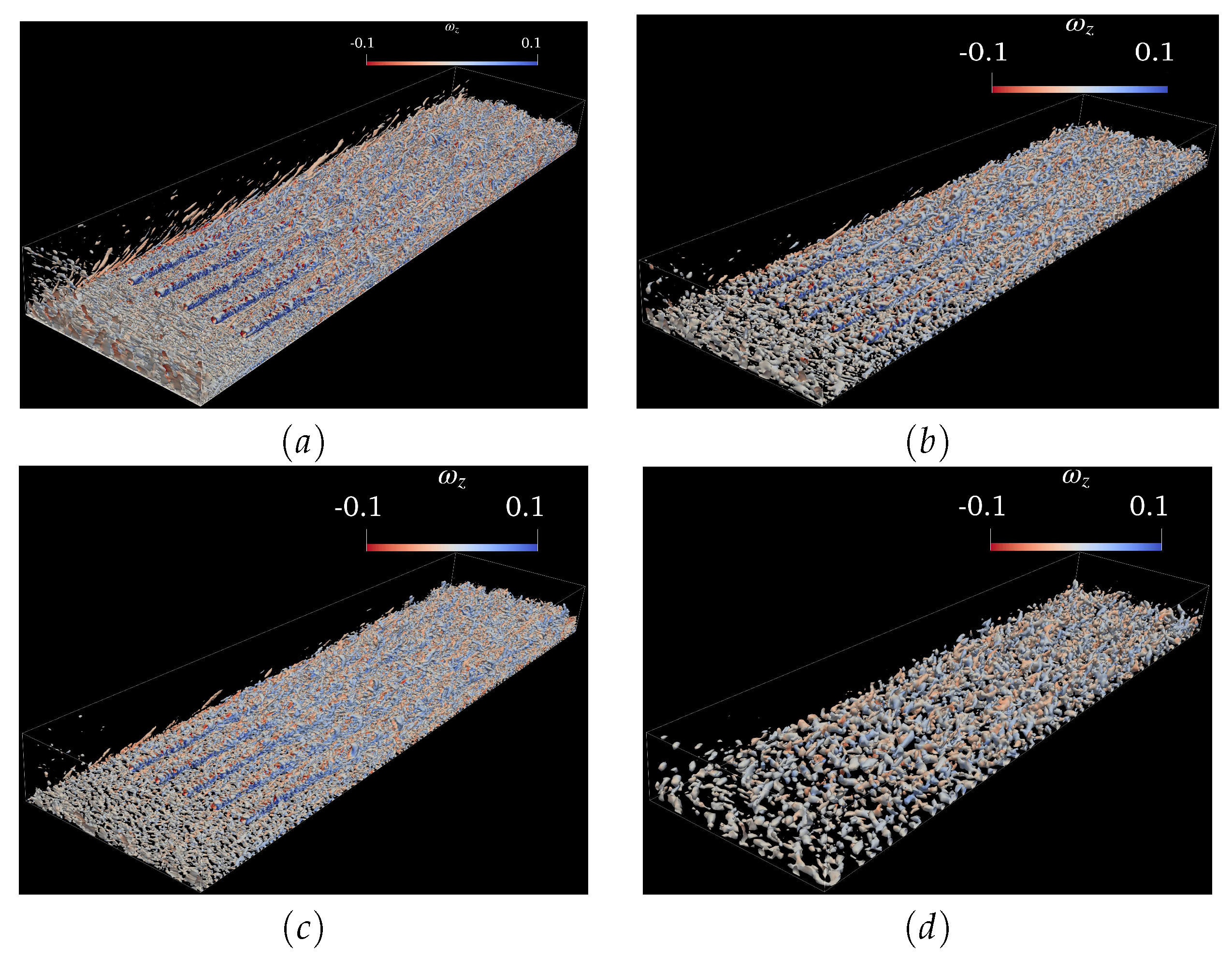
Figure 7a-d demonstrate color-filled contour plots of Q = ( 1 / 2 ) G i j G i j for Q > 0 , where the color represents the vertical vorticity ω z . The second invariant Q of the velocity gradient tensor G i j represents the relative magnitude of vorticity over strain, and thus Q > 0 identifies vortex dominated regions. Figure 7a & Figure 7c show the coherent structures and wind turbine wakes for cases M 10 and M 20 -3, respectively. Figure 7b & Figure 7d show the coherent structures in cases M 20 -1 and M 40 , respectively. For grid spacing of 20 m and 40 m, coherent structures are poorly-resolved (Figure 7b,d). When we refine the vertical grid keeping horizontal grid spacing 20 m (Figure 7c), the scale-adaptive LES method captures the coherent structures similar to case M 10 .
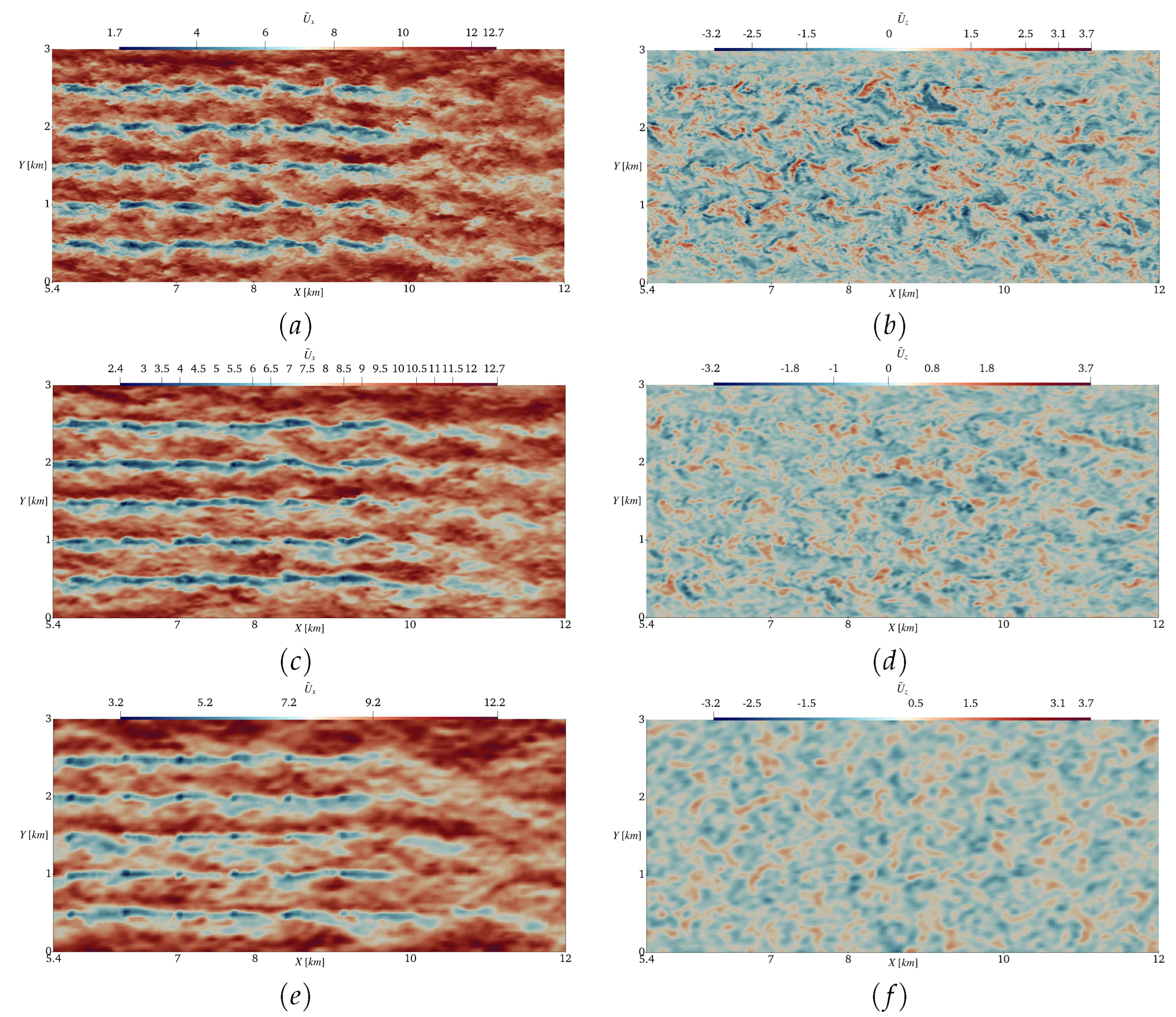
Figure 8a-f present contour plots of the streamwise and surface normal components of the resolved velocity at z = 100 m and t = 45 T * for cases M 10 , M 20 -1, and M 40 , respectively. These contour plots compare the results between one well-resolved case ( M 10 ) and two poorly-resolved cases ( M 20 -1 and M 40 ). The results indicate that the three cases equally resolve the horizontal flow structures at hub height z = 100 m.

3.2.2. Effects of resolution on the power output of the wind farm

Although Churchfield et al. [1] coupled the actuator line model with the aerodynamic structural response model, there is still a need for a computational framework capable of capturing atmosphere-turbine interactions in a realistic atmospheric environment [18,78,79]. For example, a generalized actuator disk model represents wind turbine wake effects by applying instantaneous forces to each component of the Navier-Stokes equations. Here, we employ the actuator disk theory; however, we calculate the thrust force based on the local disk-averaged velocity using a modified thrust coefficient (see [72,78]).
Thus, the power extracted by a wind turbine is
P t = 2 a / ( 1 a ) ρ A u d 3 ,
where a is the axial induction factor, ρ is the air density, A is the rotor swept area, and u d is the mean velocity at the rotor [78]. Note that local velocity u d partially accounts for the wake effect. Due to additional complexity in properly considering the effects of all the influencing parameters, it is not straightforward to evaluate wind farm performance using the equation above. If the inflow condition is fixed, wake effects are a major source of power production losses in wind farms. Vertical transport and turbulence mixing are primary mechanisms for wake recovery for turbines operating in the wake of another turbine. It is worth mentioning that the average power of large wind farms may be limited to around 1.5 Wm 2 (see [10]).
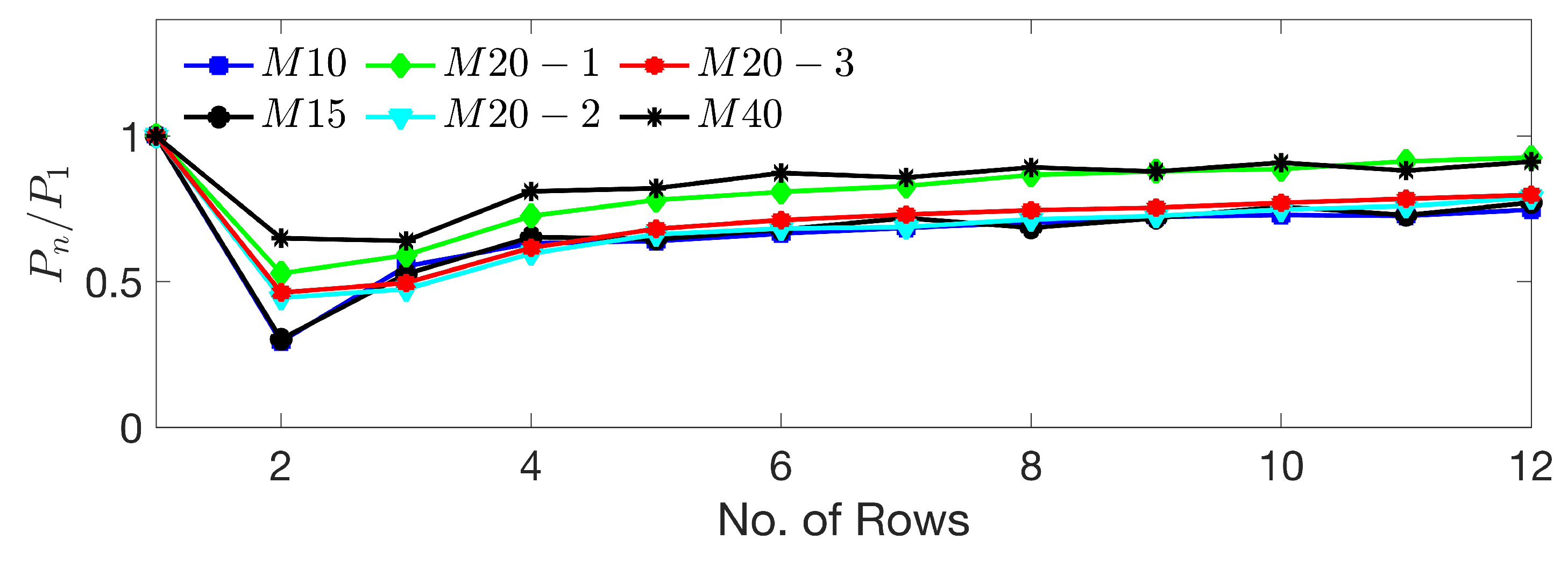
Figure 9 compares the average power of a turbine at each row with various mesh resolutions. Cases M 20 -1 and M 40 over-predict the power production, indicating the need for a finer mesh resolution; however, as we refine the vertical grid, such as in cases M 20 -2 and M 20 -3, the average power converges towards the well-resolved high-resolution case.

3.3. Effect of vertical mixing on wind farms in complex terrain

Wind speed over the hills is often higher than those in the areas over flat land [6]. However, it remains unclear whether a greater downward transport of kinetic energy may be sustained in mountainous and forested terrain [5]. The wake of a single wind turbine often exhibits reduced vertical mixing [78]. In stably stratified atmospheric conditions, temperature rise below the rotor tip suggests the downward flux may persist in large wind farms (see [17] and the refs therein). In the atmospheric boundary layer, the flux of mean kinetic energy at height z is approximately Φ ( z ) = u w ¯ u ¯ ( z ) . Using Eq (3) and assuming that u * 2 = u w ¯ , the energy flux Φ ( z ) = ( u * 3 / z 0 ) ln ( z / z 0 ) at height z increases as z 0 increases.
The geostrophic drag law relates the surface friction velocity u * (i.e. surface shear-stress τ w = u * 2 ) and the aerodynamic roughness length z 0 [32]. In meteorological applications, the geostrophic drag law assumes that the Coriolis and the pressure gradient force are in geostrophic balance, and the atmospheric background stratification is neglected. The commonly used wind profile based on geostrophic drag law for wind resource assessment is [80]
u ( z ) U g = u * k ln f z u * + C .
Here, f = 2 Ω sin ϕ represents the Coriolis force. Using Eq (7), the depth of the atmospheric boundary layer is approximated as H G 0.16 u * / f [10]. Comparing Eq (7) with the near-surface logarithmic wind profile (Eq 3), we can relate the geostrophic wind speed U g to the ground friction velocity u * as
u * = k U g ln U g f z 0 C * ,
where C * 4 [10,81]. In conditions with high wind above flexible surface protrusions, such as crops or forests, non-dimensional arguments suggest that z 0 may depend on u * as
z 0 = α c u * 2 / g ,
where α c is the Charnock’s constant and g is the gravitational constant [32]. An important observation from Eqs (8-9) is that there is a positive wind speed bias in the inertial sublayer whenever the ground roughness elements are to exert a relatively large roughness length z 0 .
Here, we simulate 10 flow fields in a wind farm considering 10 values of the neutral drag coefficient C D N = κ / ln ( z / z 0 ) 2 (as discussed in Section 2.2, Eq 5). For each of flow fields, we scatter the resolved streamwise velocity u ˜ ( x , y , z ) against the vertical coordinate z and thus, estimate u * and z 0 to get the best fit to Eq (3). Table 2 shows estimated values of z 0 and u * from these 10 velocity fields.
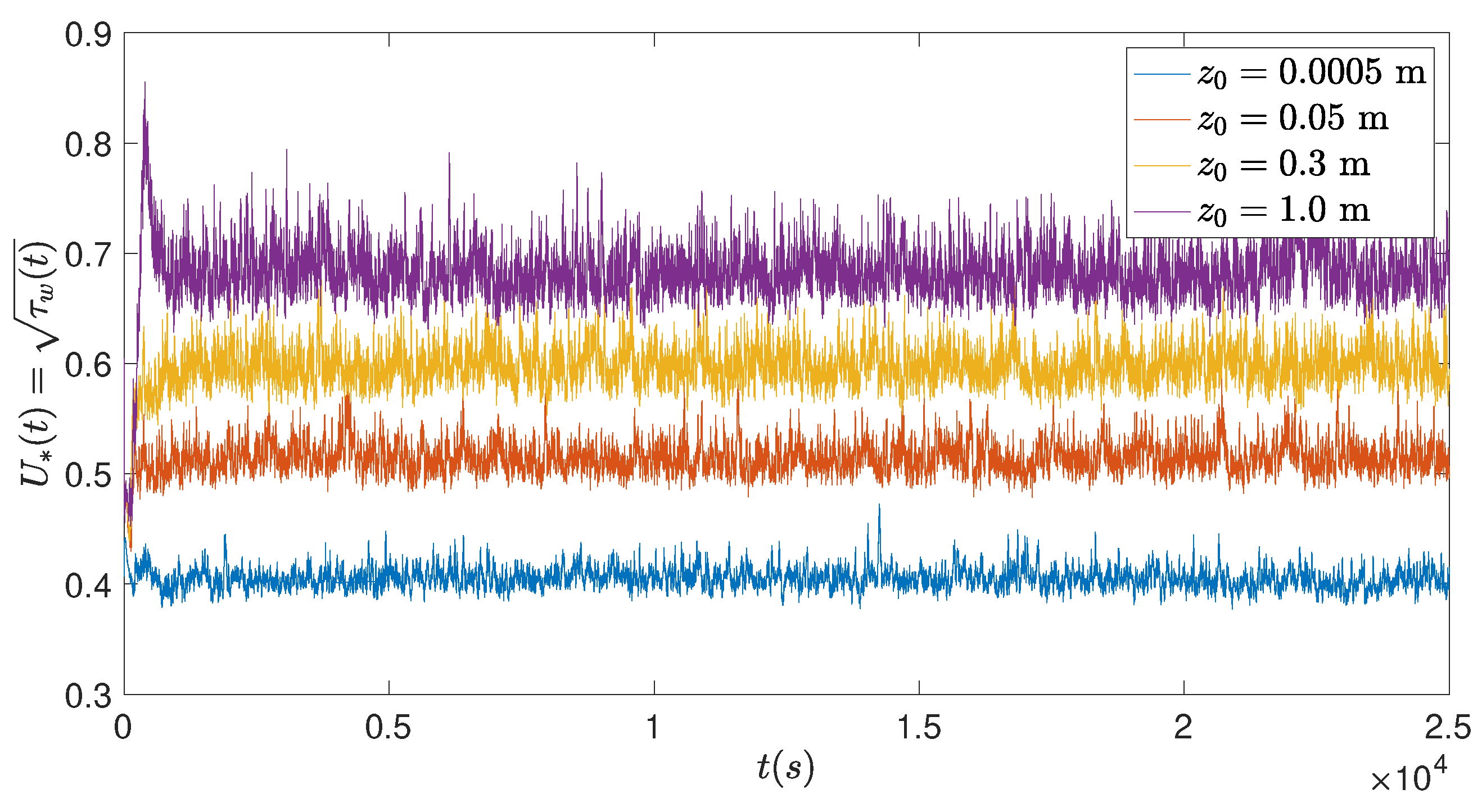
To deal with the overall effect of hills and other roughness elements, the concept of an effective roughness and effective surface force ( u * 2 , per area and normalized by density) is not new, particularly, for hills, obstacle arrays, forests, and urban canopies [17,32,50,62]. Also, several work have focused on ‘wall modelling’ [25] and ‘near surface modelling’ [29]. The present investigation’s near-surface model accounts for the complex terrain’s overall effects into the residual stress τ i j , and hence, the wall shear stress τ w ( t ) . We have analyzed 10 LES flow fields corresponding to 10 values of effective roughness length z 0 listed in Table 2 to estimate the instantaneous shear stress on the Earth’s surface, τ w ( t ) . Here, we compute the shear stress as τ w ( t ) = | | τ 13 | | 2 + | | τ 23 | | 2 , where | | τ i 3 | | = max x , y | τ i 3 ( x , y , Δ z / 2 , t ) | for i = 1 , 2 . Figure 10 shows the time evolution of the friction velocity U * ( t ) = τ w ( t ) associated with 4 values of the roughness height z 0 . Note the upper case symbol U * ( t ) for transient friction velocity. We see that a relatively smooth surface (with z 0 = 5 × 10 4 m ) produces relatively low friction velocity U * ( t ) . However, increased roughness enhances fluctuations, impacting turbulent structures and momentum flux aloft. Based on the scaling analysis of the atmospheric boundary layer [32], the influence of complex terrain on the shear stress τ w ( t ) indicates the corresponding impact on the downward flux of energy and the geophysical potential for the wind energy density.
The primary source of kinetic energy for a wind farm is the geostrophic wind in the free atmosphere, which is transferred to the wind turbine. A basic understanding of flow phenomena associated with performance loss for downstream turbines in a wind farm may lead to improvements in wind energy harvesting. For instance, consider the wake effects in the Horns Rev wind farm [79], which consists of 80 Vestas V-80 wind turbines covering an area of 20 km 2 . The layout of Horns Rev consists of an array of 10 rows and 8 columns. The rows are rotated approximately 7 degrees counterclockwise from the North-South direction. Wu and Porté-Agel [79] demonstrate wake effects in Horns Rev wind farm using LES in a domain of approximately 16 km 2 . The simulations assumed a fixed hub-height velocity ( z h = 80 m ) of 8 m / s and an aerodynamic roughness length of z 0 = 0.05 m . The LES of Horns Rev wind farm [79] provides a reference for computational studies of wind farms.
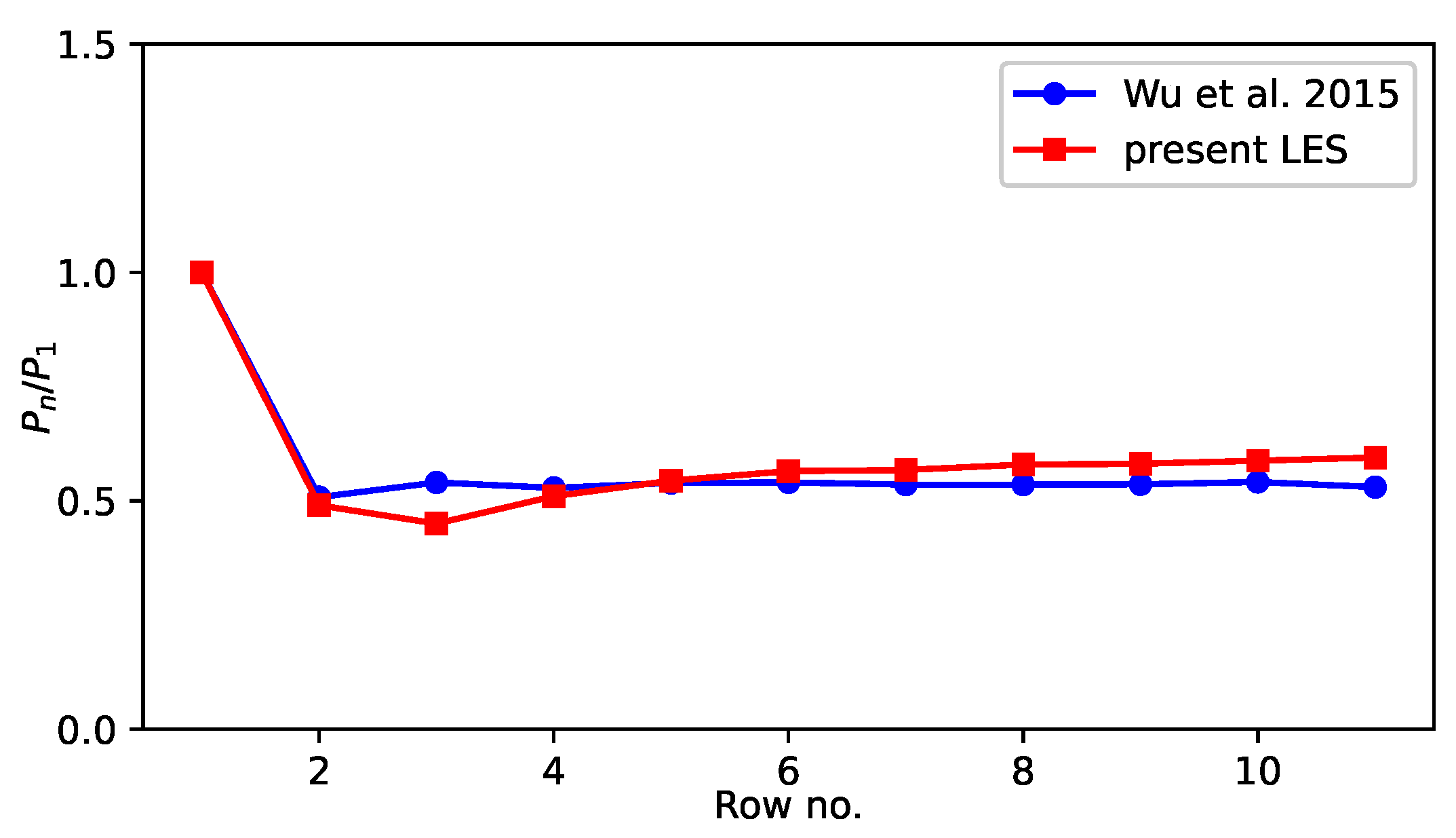
In the present study, we simulate a wind farm, where the hub height ( z h = 100 m ) wind speed is 10 m / s and the aerodynamic roughness length is z 0 = 0.05 m. The wind farm consists of an array of 12 × 5 wind turbines, covering approximately an area of 36 km 2 . Thus, the present wind farm is different than the Horns Rev wind farm (and that of Wu and Porté-Agel [79]). However, in Figure 11, we observe that the performance of the present wind farm is very similar to that of Wu and Porté-Agel [79]. Let us briefly discuss the impact of surface roughness on wind farm performance, where we varied the surface roughness between z 0 = 5 × 10 4 m and z 0 = 1.0 m. As discussed above, an increase of the overall roughness height z 0 due to hills and forests increases the downward energy flux and the wind speed in the inertial sublayer. The relative power P n / P 1 is a measure for the resulting impact on the wind farm performance, where P n is the average power extracted by a turbine at n-th row. Figure 12 compares P n / P 1 for 4 values of the roughness height z 0 . For z 0 = 5 × 10 4 m, each turbine after the third row indicates to have the same performance of approximately 40% relative to the first row. There are known reasons for such an observed performance. For instance, the partial wake recovery within the wind farm after a few rows (3 in the present study) is a geophysical potential due to the vertical flux of atmospheric turbulence. For z 0 = 1 m, the wake is recovered approximately 80% after the fifth row. Thus, the overall effect of complex terrain is likely to increase the available kinetic energy for wind turbines. Clearly, there is an enhanced momentum exchange between the land and atmosphere for a fully rough surface, resulting in more energy entrainment from aloft [1,2].
The present study does not provide a detailed analysis of the local production of turbulence kinetic energy and the associated load on wind turbines [1,6]. However, Figure 12 suggests an overall reduction of turbulence kinetic energy by complex terrain in wind farms. As we know, turbulence is highly intermittent, local production of turbulence and shear stress may be responsible for fatigue load.

3.4. Relation between power and drag coefficient

As the complexity (i.e. slope, distribution, etc) of the roughness elements increases, the drag coefficient also increases, thereby causing an increase in the roughness length z 0 [32]. Evaluating the drag coefficient from observations and identifying the variables that influence it, such as wind speed, is a costly experimental process. For a neutrally stratified atmospheric boundary layer over a fully rough surface, C D N is obtained by using Eq 5 and Eq 9:
C D N = k 2 / ln ( z g / α c u * 2 ) 2 .
Formulating a similar relationship between the power production and the drag coefficient for wind farms sited over a complex terrain would be interesting. Wind turbines may also contribute to the roughness length z 0 . In other words, the wind farm’s density and layout can affect the drag coefficient C D N , which in turn can affect the power output. The present study unveils a relationship between heterogeneous spatial surfaces and power dependence, which can be instrumental in optimizing power generation and drag in large-scale wind farms. We obtain the drag coefficient ( C D N ) from Eq 10 for each case shown in Table 2, where z 0 and u * are computed by fitting the LES data with Eq 3. We took the value of Charnock constant, α c 0.0144 [32].
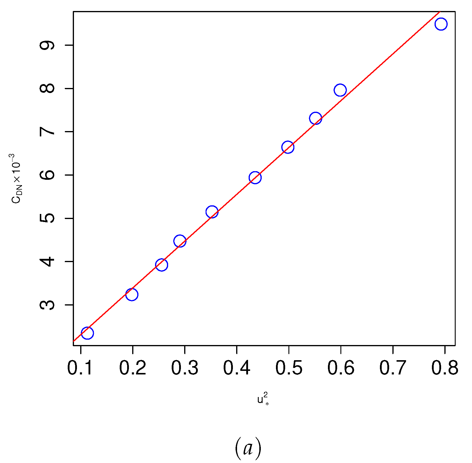
Figure 13a shows a correlation between the neutral drag coefficient C D N and the square of the friction velocity u * .
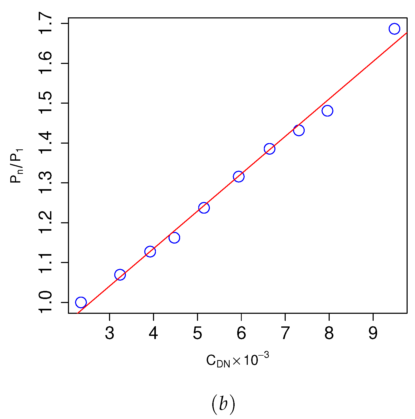
The best least square fit indicates a linear relationship between C D N and wall shear stress (i.e. squared friction velocity). This finding is consistent with Charnock’s formulation illustrating the impact of wind speed on the drag coefficient [32]. Notably, as the roughness of the terrain increases, wind speed near the ground decreases while accelerating it near the hub height or aloft and thus, leading to enhanced wind power production [6]. However, increasing the roughness of the complex terrain also increases the overall drag in the wind farm [11]. We obtain the normalized power P = P i / P 1 for each of the cases listed in Table 2, where P i is power obtained for Row 1 - 12 with i representing the row number 1 to 12. We regressed P i / P 1 against the drag coefficient C D N . Figure 13b shows the variation of the power production in a wind farm as a function of the neutral drag coefficient. The best fit linear equation for the wind power as a function of C D N is
P = ( β 1 + β 2 C D N ) × 10 3 ,
where the parameters β 1 and β 2 are approximately 0.747 and 0.114 , respectively. This relationship helps advance the analytical model for analyzing the power production of wind farms in complex terrains.

3.5. Dispersive stress analysis

Characterizing secondary turbulent motions is essential to quantify the degree of spatial heterogeneity in large wind farms. However, the turbulent transport of momentum in wind farms is a very complicated phenomena due to interaction of wind turbines and complex terrain. Here, we consider the Double-Averaged Navier-Stokes (DANS) equations to evaluate the dispersive (or form-induced) stresses, which represents the turbulent momentum transport due to spatial heterogeneity.
Let us consider the Reynolds decomposition of the solution of Eq 2:
u ˜ i ( x , t ) = u ¯ i ( x , t ) + u i ( x , t ) ,
where
u ¯ i ( x , t ) 1 N n = 1 N u ˜ i ( x , t ; n ) ,
is the time-average of N snapshots of the LES resolved velocity u ˜ i ( x , t ; n ) . In the present analysis, each snapshot is the velocity at n-th time step with CFL=1. The number of snapshot ( N ) is large enough to capture the flow for a duration of 45 eddy turn over time units at a sampling rate of 1 Hz, yet average velocity varies slowly in time. Next, we consider the spatial averaging of the time-averaged velocity field,
u ¯ i = 1 A u ¯ ( x , t ) d x d y ,
where A is the area of a horizontal plane parallel to the ground surface at z = 0 . The application of the dual operation of time and spatial averaging in Eq 12 & Eq 13 results in the triple decomposition of the LES resolved field u i ˜ ( x , t ) . Thus, we have
u ˜ i ( x , t ) u ¯ i + u i ( x , t ) u ¯ i ( x , t ) + u i ( x , t ) .
According to the above decomposition, the dispersive stress associated with the horizontal spatial averaging is
D i j ( z ) ( u ¯ i u ¯ i ) ( u ¯ j u ¯ j ) = u i u j .
Note, however, that the Reynolds stress is due to the joint variability of the randomness between the velocity fluctuations,
R i j ( x ) = ( u i ˜ u ¯ i ) ( u j ˜ u ¯ j ) ¯ = u i u j ¯ .
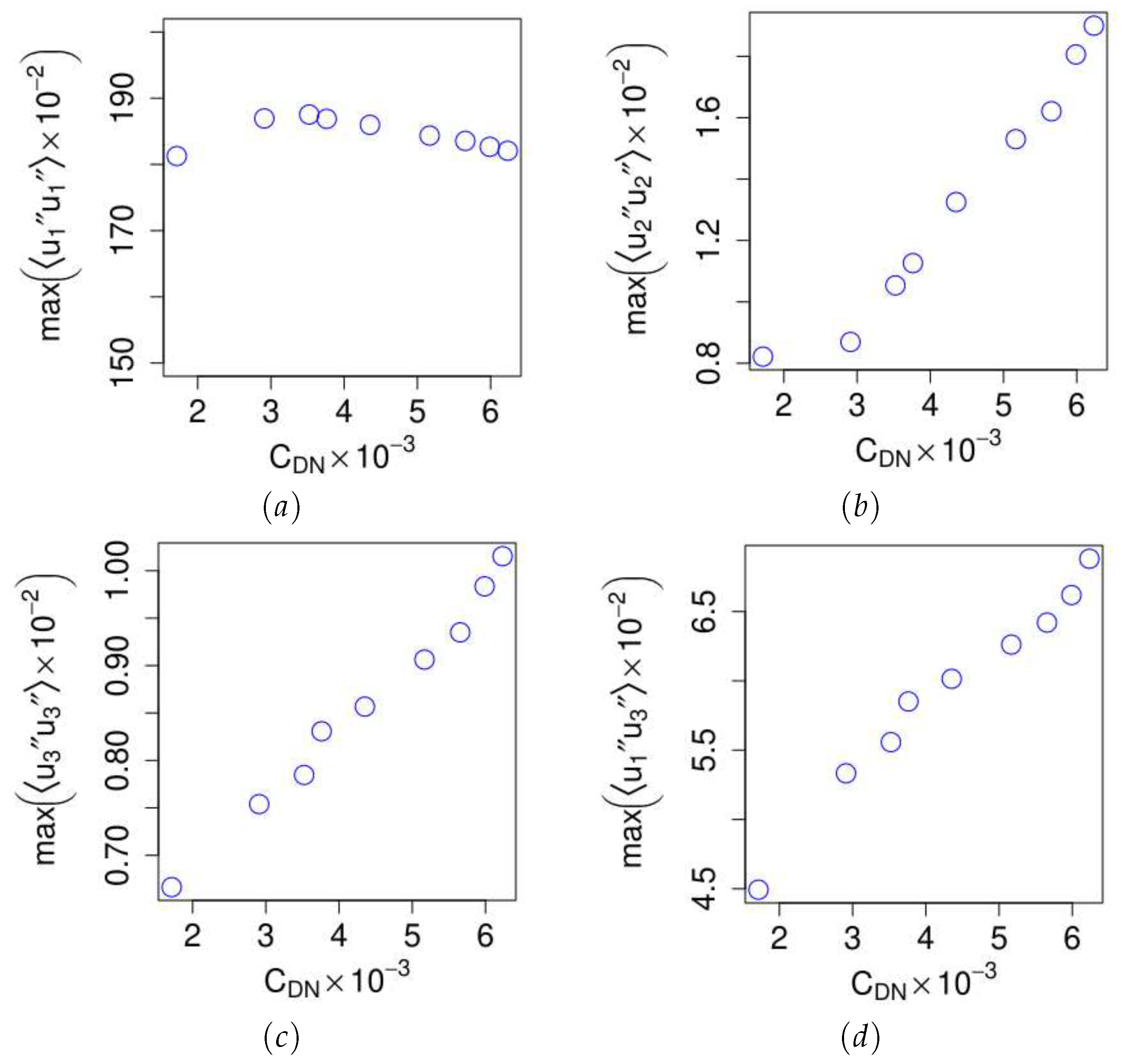
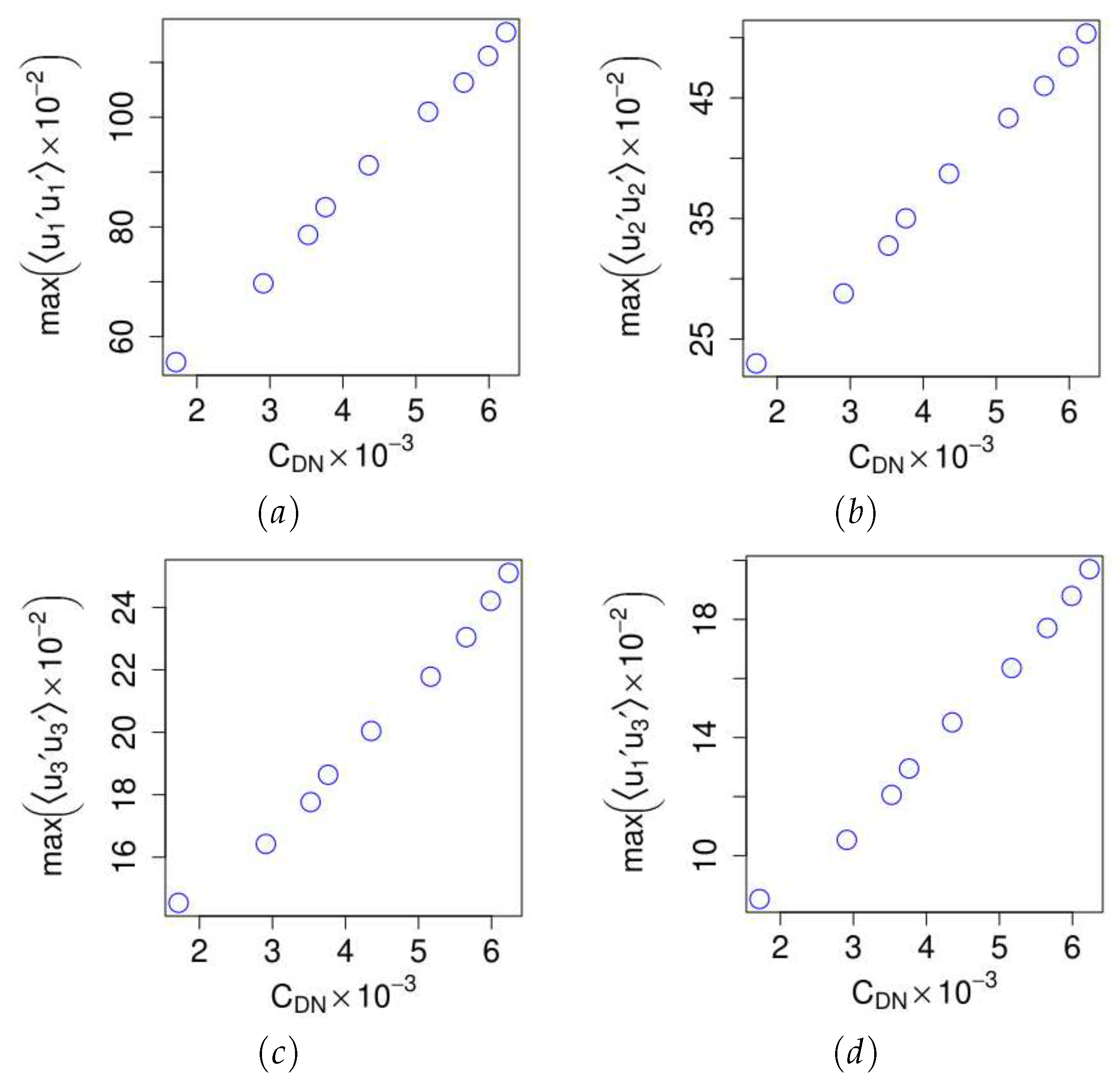
We have computed the dispersive, and the Reynolds stresses using Eq 15 and Eq 16, respectively, and compare their relative contributions to the total drag. We obtained the maximum value of the stresses as a function of the drag coefficient C D N (See Eq 10). Figure 14 shows the variations of dispersive stress components with respect to the drag coefficient. The first notable observation from Figure 14a is that the streamwise normal component u 1 u 1 of the dispersive stress is relatively insensitive to the drag coefficient. However, the spanwise u 2 u 2 and surface-normal components u 3 u 3 vary linearly with the drag coefficient (Figure 14b and Figure 14c). In contrast, the corresponding Reynolds stresses vary linearly with the drag coefficient, as shown in Figure 15. It is interesting to note that the magnitude of the streamwise component of dispersive stress u 1 u 1 is higher than its Reynolds stress u 1 u 1 ¯ counterpart. This result suggests that the dominant source of spatial heterogeneity within a wind farm is in the streamwise direction, which are the dominant "wake-occupied" regions. Additionally, the dispersive stress shows minimum variations because the present study considers an aligned arrangement of 60 wind turbines. Further research could explore this idea by quantifying the degree of spatial heterogeneity with different layouts and numbers of wind turbines and by resolving the complex terrain. Furthermore, the relative contribution of the dispersive shear stress component u 1 u 3 is almost 45 % that of the Reynolds shear stress to the drag.

4. Conclusion

This article presents a scale-adaptive LES of wind farms in complex terrain, incorporating a near-surface model. Using the LES data of an idealized wind farm, we have analyzed the impact of complex mountainous terrain on the performance of wind farms, where the simulation does not explicitly resolve the shape of the mountain or other roughness elements. We observe that the near-surface model helps improve the accuracy of capturing the atmospheric boundary layer turbulence without needing an extremely refined mesh. We investigated the effect of grid resolution on the ABL and wake profiles and observed that the ABL wind profile is not very sensitive to grid resolution, whereas the wake profile depends on grid resolutions. When the grid has about ten grid points across the rotor, at least in the vertical direction, the wake profiles converge according to the grid refinement analysis.
Our findings indicate a 68% increase in normalized power production in wind farms situated in mountainous and forested terrain compared to a flat or offshore location. This study treats the subgrid-scale effects of terrain complexity without resolving the shape of roughness elements. We observe a linear correlation between the power production and the drag coefficient and show that drag increases as the surface roughness of the terrain increases. These findings help us understand the consequences of atmospheric turbulence on the performance of wind farms.
We provide a quantitative assessment of the secondary motion due to spatial heterogeneity in onshore sites of wind farms. We analyze the dispersive and Reynolds stresses. We follow the double-averaged Navier-Stokes equations to formulate the dispersive stresses. We show that a dominant source impacting a wind farm through spatial heterogeneity is due to the incoming turbulent flow, where the wind turbines are perpendicular to the streamwise direction. Furthermore, we observed that the dispersive shear stress contributes nearly 45% of the drag of wind farms in complex terrain compared to the Reynolds shear stress.
The development of wind farms in complex terrain poses significant challenges. The site assessment requires assessing performance due to the interaction of wind turbine wakes and atmospheric boundary layer flow. Different from flat terrain, it is challenging to characterize the complex terrain’s wind patterns because measurements at one point may not represent the flow state at points only a few hundred meters away. The present study highlights the importance of accurately modelling the subgrid-scale effects of the secondary motion due to the spatial heterogeneity imposed by the complex terrain. Future research may focus on capturing the grid-scale variation of the topography while modelling the relevant subgrid-scale effects. There are two crucial questions. Can artificial windbreaks be considered to compensate for the blockage of mountains on the reduced performance of turbines? If trees can provide potential windbreaks, it would be interesting to characterize the optimal placement of trees on mountainous terrain. Mountain and internal waves are essential to assess the potential role of atmospheric turbulence on wind farms in complex terrain. Since the middle of the twentieth century, the atmospheric science community has confirmed that complex terrain substantially impacts large-scale circulation and stationary waves, subsequently affecting the regional climate. Suppose we aim for global net-zero emissions by 2050 in the context of 1.5 degrees change scenario. In that case, we must incorporate such a large-scale effect of mountains in optimizing the wind farm layout.

References

  1. Churchfield, M.J.; Lee, S.; Michalakes, J.; Moriarty, P.J. A numerical study of the effects of atmospheric and wake turbulence on wind turbine dynamics. Journal of turbulence 2012, 13, N14. [Google Scholar] [CrossRef]
  2. Vanderwende, B.; Lundquist, J.K. Could crop height affect the wind resource at agriculturally productive wind farm sites? Boundary-Layer Meteorology 2016, 158, 409–428. [Google Scholar] [CrossRef]
  3. Pan, Y.; Archer, C.L. A Hybrid Wind-Farm Parametrization for Mesoscale and Climate Models. Boundary-Layer Meteorology 2018, 168, 469–495. [Google Scholar] [CrossRef]
  4. Porté-Agel, F.; Bastankhah, M.; Shamsoddin, S. Wind-turbine and wind-farm flows: a review. Boundary-Layer Meteorology 2020, 174, 1–59. [Google Scholar] [CrossRef]
  5. Alfredsson, P.H.; Segalini, A. Introduction Wind farms in complex terrains: an introduction, 2017.
  6. Tian, W.; Ozbay, A.; Yuan, W.; Sarakar, P.; Hu, H.; Yuan, W. An experimental study on the performances of wind turbines over complex terrain. 51st Am Inst Aeronaut Astronaut Aerospace Sci. Mtg, Grapevine, Texas, USA, 2013. [Google Scholar]
  7. Yang, X.; Pakula, M.; Sotiropoulos, F. Large-eddy simulation of a utility-scale wind farm in complex terrain. Applied energy 2018, 229, 767–777. [Google Scholar] [CrossRef]
  8. Liu, L.; Stevens, R.J. Enhanced wind-farm performance using windbreaks. Physical review fluids 2021, 6, 074611. [Google Scholar] [CrossRef]
  9. Zhang, Z.; Huang, P.; Bitsuamlak, G.; Cao, S. Large-eddy simulation of wind-turbine wakes over two-dimensional hills. Physics of Fluids 2022, 34. [Google Scholar] [CrossRef]
  10. Calaf, M.; Meneveau, C.; Meyers, J. Large eddy simulation study of fully developed wind-turbine array boundary layers. Physics of fluids 2010, 22, 015110. [Google Scholar] [CrossRef]
  11. Tobin, N.; Chamorro, L.P. Windbreak effects within infinite wind farms. Energies 2017, 10, 1140. [Google Scholar] [CrossRef]
  12. Mahrer, Y. An improved numerical approximation of the horizontal gradients in a terrain-following coordinate system. Monthly weather review 1984, 112, 918–922. [Google Scholar] [CrossRef]
  13. Lundquist, K.A.; Chow, F.K.; Lundquist, J.K. An Immersed Boundary Method for the Weather Research and Forecasting Model. Monthly Weather Review 2010, 138, 796–817. [Google Scholar] [CrossRef]
  14. Lundquist, K.A.; Chow, F.K.; Lundquist, J.K. An immersed boundary method enabling large-eddy simulations of flow over complex terrain in the WRF model. Monthly Weather Review 2012, 140, 3936–3955. [Google Scholar] [CrossRef]
  15. Arthur, R.S.; Mirocha, J.D.; Lundquist, K.A.; Street, R.L. Using a canopy model framework to improve large-eddy simulations of the neutral atmospheric boundary layer in the Weather Research and Forecasting Model. Monthly Weather Review 2019, 147, 31–52. [Google Scholar] [CrossRef]
  16. Bhuiyan, M.A.S.; Alam, J.M. Scale-adaptive turbulence modeling for LES over complex terrain. Engineering with Computers 2020, 1–13. [Google Scholar] [CrossRef]
  17. Alam, J. Interaction of vortex stretching with wind power fluctuations. Physics of Fluids 2022, 34, 075132. [Google Scholar] [CrossRef]
  18. Stevens, R.; Meneveau, C. Flow structure and turbulence in wind farms. Annu. Rev. Fluid Mech 2017, 49, 311–339. [Google Scholar] [CrossRef]
  19. Xie, S.; Archer, C.L. A numerical study of wind-turbine wakes for three atmospheric stability conditions. Boundary-Layer Meteorology 2017, 165, 87–112. [Google Scholar] [CrossRef]
  20. Abedi, H. Assessment of flow characteristics over complex terrain covered by the heterogeneous forest at slightly varying mean flow directions:(A case study of a Swedish wind farm). Renewable Energy 2023, 202, 537–553. [Google Scholar] [CrossRef]
  21. Bao, J.; Chow, F.K.; Lundquist, K.A. Large-eddy simulation over complex terrain using an improved immersed boundary method in the Weather Research and Forecasting Model. Monthly Weather Review 2018, 146, 2781–2797. [Google Scholar] [CrossRef]
  22. Moeng, C.H. A large-eddy-simulation model for the study of planetary boundary-layer turbulence. Journal of the Atmospheric Sciences 1984, 41, 2052–2062. [Google Scholar] [CrossRef]
  23. Moeng, C.H.; Sullivan, P.P. A comparison of shear-and buoyancy-driven planetary boundary layer flows. Journal of Atmospheric Sciences 1994, 51, 999–1022. [Google Scholar] [CrossRef]
  24. Porté-Agel, F.; Meneveau, C.; Parlange, M.B. A scale-dependent dynamic model for large-eddy simulation: application to a neutral atmospheric boundary layer. Journal of Fluid Mechanics 2000, 415, 261–284. [Google Scholar] [CrossRef]
  25. Bose, S.T.; Park, G.I. Wall-modeled large-eddy simulation for complex turbulent flows. Annual review of fluid mechanics 2018, 50, 535–561. [Google Scholar] [CrossRef] [PubMed]
  26. Chow, F.K.; Schär, C.; Ban, N.; Lundquist, K.A.; Schlemmer, L.; Shi, X. Crossing Multiple Gray Zones in the Transition from Mesoscale to Microscale Simulation over Complex Terrain. Atmosphere 2019, 10. [Google Scholar] [CrossRef]
  27. Goodfriend, E.; Katopodes Chow, F.; Vanella, M.; Balaras, E. Large-Eddy Simulation of Flow Through an Array of Cubes with Local Grid Refinement. Boundary-Layer Meteorology 2016, 159, 285–303. [Google Scholar] [CrossRef]
  28. Mason, P.J.; Thomson, D.J. Stochastic backscatter in large-eddy simulations of boundary layers. Journal of Fluid Mechanics 1992, 242, 51–78. [Google Scholar] [CrossRef]
  29. Senocak, I.; Ackerman, A.S.; Kirkpatrick, M.P.; Stevens, D.E.; Mansour, N.N. Study of near-surface models for large-eddy simulations of a neutrally stratified atmospheric boundary layer. Boundary-layer meteorology 2007, 124, 405–424. [Google Scholar] [CrossRef]
  30. Johnson, P.L. On the role of vorticity stretching and strain self-amplification in the turbulence energy cascade. Journal of Fluid Mechanics 2021, 922, A3. [Google Scholar] [CrossRef]
  31. Hossen, M.K.; Mulayath-Variyath, A.; Alam, J. Statistical Analysis of Dynamic Subgrid Modeling Approaches in Large Eddy Simulation, 2021. [CrossRef]
  32. Garratt, J. The Atmospheric Boundary Layer; Cambridge University Press, 1994. [Google Scholar]
  33. Stull, R.B.; Ahrens, C.D.; et al. Meteorology for scientists and engineers; Brooks/Cole, 2000. [Google Scholar]
  34. Blom, J.; Wartena, L. The influence of changes in surface roughness on the development of the turbulent boundary layer in the lower layers of the atmosphere. Journal of the Atmospheric Sciences 1969, 26, 255–265. [Google Scholar] [CrossRef]
  35. Nickerson, E.C.; Smiley, V.E. Surface layer and energy budget parameterizations for mesoscale models. Journal of Applied Meteorology (1962-1982) 1975, 297–300. [Google Scholar] [CrossRef]
  36. Ye, C.; Liu, X.n.; Wang, X.k. Effects of roughness elements distribution on overland flow resistance. Journal of Mountain Science 2015, 12, 1145–1156. [Google Scholar] [CrossRef]
  37. Tani, I.; Sato, H. Boundary-layer transition by roughness element. Journal of the Physical Society of Japan 1956, 11, 1284–1291. [Google Scholar] [CrossRef]
  38. Irwin, J.S. A theoretical variation of the wind profile power-law exponent as a function of surface roughness and stability. Atmospheric Environment (1967) 1979, 13, 191–194. [Google Scholar] [CrossRef]
  39. Essa, K.S.; Embaby, M.; Etman, S.M. A notional variation of the wind profile power-law exponent as a function of surface roughness and stability. 2004.
  40. Cao, S.; Wang, T.; Ge, Y.; Tamura, Y. Numerical study on turbulent boundary layers over two-dimensional hills—effects of surface roughness and slope. Journal of wind engineering and industrial aerodynamics 2012, 104, 342–349. [Google Scholar] [CrossRef]
  41. De Paepe, W.; Pindado, S.; Bram, S.; Contino, F. Simplified elements for wind-tunnel measurements with type-III-terrain atmospheric boundary layer. Measurement 2016, 91, 590–600. [Google Scholar] [CrossRef]
  42. Finnigan, J.; Ayotte, K.; Harman, I.; Katul, G.; Oldroyd, H.; Patton, E.; Poggi, D.; Ross, A.; Taylor, P. Boundary-layer flow over complex topography. Boundary-Layer Meteorology 2020, 177, 247–313. [Google Scholar] [CrossRef]
  43. Tobin, N.; Hamed, A.M.; Chamorro, L.P. Fractional flow speed-up from porous windbreaks for enhanced wind-turbine power. Boundary-Layer Meteorology 2017, 163, 253–271. [Google Scholar] [CrossRef]
  44. Zhang, Y. GROUND SURFACE EFFECTS IN WIND FARMS: A MICRO WIND FARM MODEL STUDY. PhD thesis, Johns Hopkins University, 2018. [Google Scholar]
  45. Mattuella, J.; Loredo-Souza, A.; Oliveira, M.; Petry, A. Wind tunnel experimental analysis of a complex terrain micrositing. Renewable and Sustainable Energy Reviews 2016, 54, 110–119. [Google Scholar] [CrossRef]
  46. Cheng, S.; Elgendi, M.; Lu, F.; Chamorro, L.P. On the wind turbine wake and forest terrain interaction. Energies 2021, 14, 7204. [Google Scholar] [CrossRef]
  47. Yang, D.; Meneveau, C.; Shen, L. Large-eddy simulation of offshore wind farm. Physics of Fluids 2014, 26, 025101. [Google Scholar] [CrossRef]
  48. Modesti, D.; Pirozzoli, S.; Orlandi, P.; Grasso, F. On the role of secondary motions in turbulent square duct flow. Journal of Fluid Mechanics 2018, 847. [Google Scholar] [CrossRef]
  49. Moltchanov, S.; Shavit, U. A phenomenological closure model of the normal dispersive stresses. Water Resources Research 2013, 49, 8222–8233. [Google Scholar] [CrossRef]
  50. Raupach, M.R.; Shaw, R. Averaging procedures for flow within vegetation canopies. Boundary-layer meteorology 1982, 22, 79–90. [Google Scholar] [CrossRef]
  51. Raupach, M.; Coppin, P.; Legg, B. Experiments on scalar dispersion within a model plant canopy part I: The turbulence structure. Boundary-Layer Meteorology 1986, 35, 21–52. [Google Scholar] [CrossRef]
  52. Böhm, M.; Finnigan, J.; Raupach, M. Dispersive fluxes and canopy flows: Just how important are they? 2000.
  53. Poggi, D.; Katul, G.; Albertson, J. A note on the contribution of dispersive fluxes to momentum transfer within canopies. Boundary-layer meteorology 2004, 111, 615–621. [Google Scholar] [CrossRef]
  54. Coceal, O.; Thomas, T.; Castro, I.; Belcher, S. Mean flow and turbulence statistics over groups of urban-like cubical obstacles. Boundary-Layer Meteorology 2006, 121, 491–519. [Google Scholar] [CrossRef]
  55. Giménez-Curto, L.A.; Lera, M.A.C. Oscillating turbulent flow over very rough surfaces. Journal of Geophysical Research: Oceans 1996, 101, 20745–20758. [Google Scholar] [CrossRef]
  56. Cheng, H.; Castro, I.P. Near wall flow over urban-like roughness. Boundary-Layer Meteorology 2002, 104, 229–259. [Google Scholar] [CrossRef]
  57. Santiago, J.L.; Martilli, A.; Martín, F. CFD simulation of airflow over a regular array of cubes. Part I: Three-dimensional simulation of the flow and validation with wind-tunnel measurements. Boundary-layer meteorology 2007, 122, 609–634. [Google Scholar] [CrossRef]
  58. Pokrajac, D.; Campbell, L.J.; Nikora, V.; Manes, C.; McEwan, I. Quadrant analysis of persistent spatial velocity perturbations over square-bar roughness. Experiments in fluids 2007, 42, 413–423. [Google Scholar] [CrossRef]
  59. Manes, C.; Pokrajac, D.; Coceal, O.; McEWAN, I. On the significance of form-induced stress in rough wall turbulent boundary layers. Acta Geophysica 2008, 56, 845–861. [Google Scholar] [CrossRef]
  60. Jelly, T.O.; Busse, A. Reynolds number dependence of Reynolds and dispersive stresses in turbulent channel flow past irregular near-Gaussian roughness. International Journal of Heat and Fluid Flow 2019, 80, 108485. [Google Scholar] [CrossRef]
  61. Toussaint, D.; Chedevergne, F.; Léon, O. Analysis of the different sources of stress acting in fully rough turbulent flows over geometrical roughness elements. Physics of Fluids 2020, 32, 075107. [Google Scholar] [CrossRef]
  62. Alam, J.M.; Fitzpatrick, L.P. Large eddy simulation of flow through a periodic array of urban-like obstacles using a canopy stress method. Computers & Fluids 2018, 171, 65–78. [Google Scholar]
  63. Borue, V.; Orszag, S.A. Local energy flux and subgrid-scale statistics in three-dimensional turbulence. Journal of Fluid Mechanics 1998, 366, 1–31. [Google Scholar] [CrossRef]
  64. Johnson, P.L. Energy Transfer from Large to Small Scales in Turbulence by Multiscale Nonlinear Strain and Vorticity Interactions. Phys. Rev. Lett. 2020, 124, 104501. [Google Scholar] [CrossRef]
  65. Wurps, H.; Steinfeld, G.; Heinz, S. Grid-resolution requirements for large-eddy simulations of the atmospheric boundary layer. Boundary-Layer Meteorology 2020, 1–23. [Google Scholar] [CrossRef]
  66. Sullivan, P.P.; McWilliams, J.C.; Moeng, C.H. A subgrid-scale model for large-eddy simulation of planetary boundary-layer flows. Boundary-Layer Meteorology 1994, 71, 247–276. [Google Scholar] [CrossRef]
  67. Basu, S.; Lacser, A. A cautionary note on the use of Monin-Obukhov similarity theory in very high-resolution large-eddy simulations. Boundary-Layer Meteorology: an international journal of physical and biological processes in the atmospheric boundary layer 2017, 163, 351–355. [Google Scholar] [CrossRef]
  68. Pope, S.B. Turbulent flows; IOP Publishing, 2001. [Google Scholar]
  69. Pope, S.B. Ten questions concerning the large-eddy simulation of turbulent flows. New journal of Physics 2004, 6, 35. [Google Scholar] [CrossRef]
  70. Schumann, U. Subgrid scale model for finite difference simulations of turbulent flows in plane channels and annuli. Journal of computational physics 1975, 18, 376–404. [Google Scholar] [CrossRef]
  71. Bhuiyan, M.; Samad, A.; Alam, J.M. Large Eddy Simulation of Turbulent Flow Over a Hill Using a Canopy Stress Model. In Proceedings of the International Conference on Applied Mathematics, Modeling and Computational Science; Springer, 2017; pp. 151–160. [Google Scholar]
  72. Singh, J.; Alam, J. Dynamic modelling of near-surface turbulence in large eddy simulation of wind farms. arXiv preprint 2022, arXiv:2205.00352 2022. [Google Scholar]
  73. Medici, D.; Ivanell, S.; Dahlberg, J.Å.; Alfredsson, P.H. The upstream flow of a wind turbine: blockage effect. Wind Energy 2011, 14, 691–697. [Google Scholar] [CrossRef]
  74. Simley, E.; Angelou, N.; Mikkelsen, T.; Sjöholm, M.; Mann, J.; Pao, L.Y. Characterization of wind velocities in the upstream induction zone of a wind turbine using scanning continuous-wave lidars. Journal of Renewable and Sustainable Energy 2016, 8, 013301. [Google Scholar] [CrossRef]
  75. Strickland, J.M.; Stevens, R.J. Investigating wind farm blockage in a neutral boundary layer using large-eddy simulations. European Journal of Mechanics-B/Fluids 2022, 95, 303–314. [Google Scholar] [CrossRef]
  76. Chow, F.K.; Moin, P. A further study of numerical errors in large-eddy simulations. Journal of Computational Physics 2003, 184, 366–380. [Google Scholar] [CrossRef]
  77. Celik, I.; Cehreli, Z.; Yavuz, I. Index of resolution quality for large eddy simulations. 2005.
  78. Stevens, R.J.A.M.; Martínez-Tossas, L.A.; Meneveau, C. Comparison of wind farm large eddy simulations using actuator disk and actuator line models with wind tunnel experiments. Renewable energy 2018, 116, 470–478. [Google Scholar] [CrossRef]
  79. Wu, Y.T.; Porté-Agel, F. Modeling turbine wakes and power losses within a wind farm using LES: An application to the Horns Rev offshore wind farm. Renewable Energy 2015, 75, 945–955. [Google Scholar] [CrossRef]
  80. Frandsen, S.; Barthelmie, R.; Pryor, S.; Rathmann, O.; Larsen, S.; Højstrup, J.; Thøgersen, M. Analytical modelling of wind speed deficit in large offshore wind farms. Wind Energy: An International Journal for Progress and Applications in Wind Power Conversion Technology 2006, 9, 39–53. [Google Scholar] [CrossRef]
  81. Tennekes, H.; Lumley, J.L.; Lumley, J.L.; et al. A first course in turbulence; MIT press, 1972. [Google Scholar]
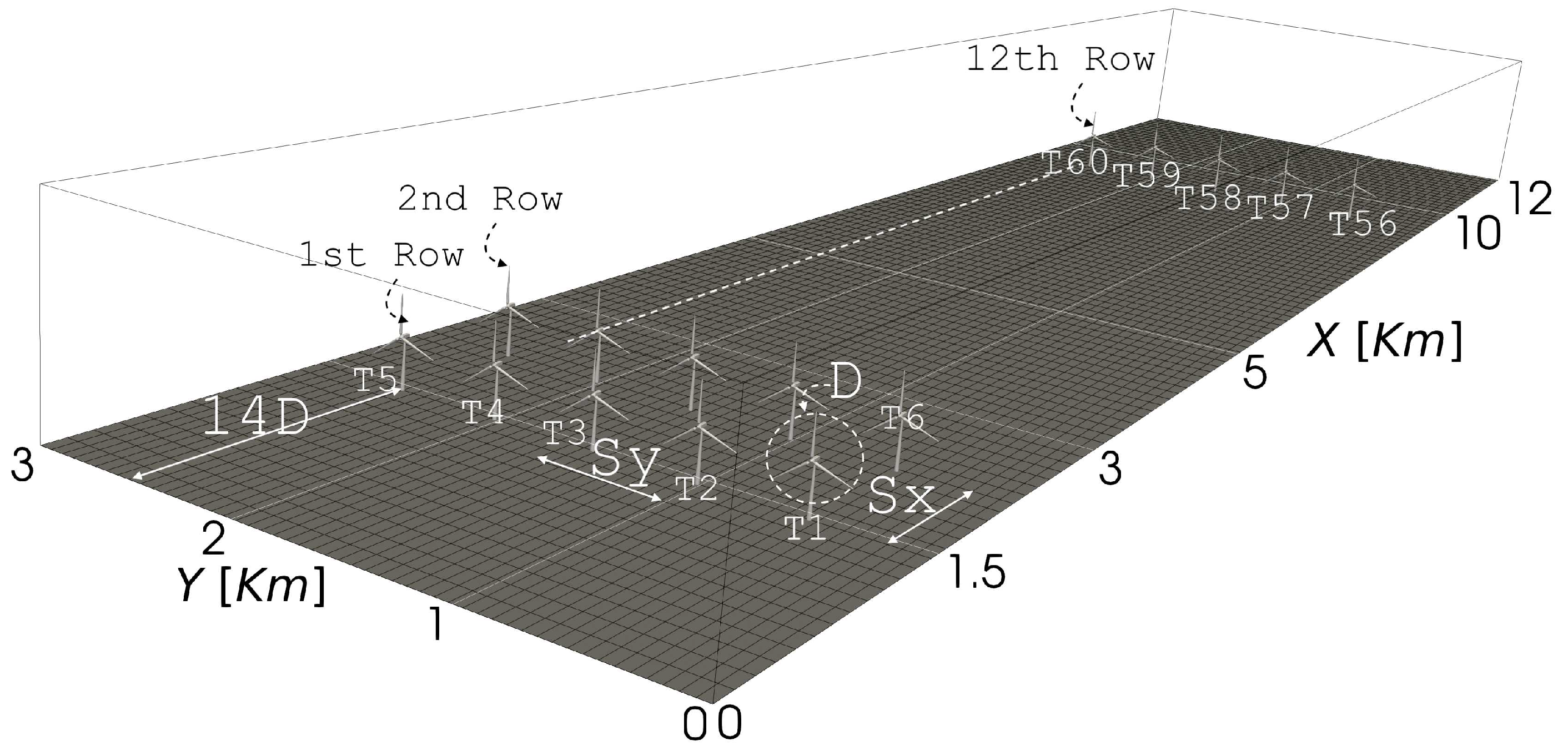
Figure 1. Schematic of the computational domain used for LES study of a 12 × 5 wind turbines for the wind farm simulations. Sketch only shows the first two and the last row for clarity. The labels T1, T2, etc., represent the center of the rotor for turbines.
Preprints 79003 g001
Figure 2. The time series of the streamwise components of the resolved velocity at three locations, ( x , y , z ) = ( 12 D , y , 1 D ) , where (from top to bottom) the spanwise coordinate of these points are same as that of the centers of three turbines at T2, T3, and T4, respectively. The bottom plot shows the time series corresponding to T2 turbine, where a moving average with a window of 512 [s] was applied.
Preprints 79003 g002
Figure 3. The figure shows the simulated wind profiles of the neutral atmospheric boundary layer for various resolutions, as indicated in Table 1. Plot (a) displays the vertical mean wind profiles, while plot (b) presents the same profiles on a logarithmic scale.
Preprints 79003 g003
Figure 4. A comparison of mesh resolution effect on wake profiles, which in the present figure is the vertical profiles of mean streamwise velocity sampled from the center column of a wind farm. The panel from left to right represents the sampling location of velocity profiles at x / D = 2 , x / D = 3 , x / D = 4 , and x / D = 5 , and top to bottom panel corresponds to a different row number ranging from 1 to 4.
Preprints 79003 g004
Figure 5. A comparison of mesh resolution effect on wake profiles. The panel from left to right represents the sampling location of velocity profiles at x / D = 2 , x / D = 3 , x / D = 4 , and x / D = 5 , and top to bottom panel corresponds to a different row number, specifically, rows 5, 7, 10, and 12.
Preprints 79003 g005
Figure 6. The figure presents the results of standard LES resolution criteria, showing (a) profiles of the squared friction velocity u * 2 , (b) the resolved portion of kinetic energy k r e s , (c) the subgrid-scale portion of kinetic energy k s g s , and (d) Effective resolution γ .
Preprints 79003 g006
Figure 7. Effect of different grid resolutions on the vortex system, computed with the Q-criterion and colored by the vertical component of vorticity ( ω z ). The top panel from left to right shows the vortex system for cases M 10 ( Δ = 10 m ) and M 20 -1 ( Δ = 20 m ), while the bottom panel shows the vortex system for cases M 20 -3 ( Δ x = Δ y = 20 m and Δ z = 8 m ) and M 40 ( Δ = 40 m ).
Preprints 79003 g007
Figure 8. Contours of streamwise and surface-normal velocity components at hub-height 100 m. The top panel ( a & b ) shows the velocity components when the grid size ( Δ ) is 10 m. Middle ( c & d ) and bottom panel ( e & f ) shows the contours when the grid size ( Δ ) is 20 m and 40 m, respectively.
Preprints 79003 g008
Figure 9. The effect of mesh resolution on wind power, which is averaged over a time interval [ 0 T sim ] , where P ¯ w t = ( 1 / T ) 0 T P ( t ) d t is the power per turbine. For each row, P ¯ w t is also averaged with respect to the number of turbines for a corresponding row which is denoted by P n , which is normalized with the power of the first row P 1 .
Preprints 79003 g009
Figure 10. Time evolution of the friction velocity ( u * ). The different profiles of friction velocity correspond to surface roughness values of z 0 = 5 × 10 4 m , z 0 = 0.05 m , z 0 = 0.3 m , and z 0 = 1.0 m .
Preprints 79003 g010
Figure 11. A comparison of normalized power distribution of simulated wind farm with present LES and LES data from Ref [79].
Preprints 79003 g011
Figure 12. The effect of complex terrain on wind power, which is averaged over a time interval [ 0 T sim ] , where P ¯ w t = ( 1 / T ) 0 T P ( t ) d t is the power per turbine. For each row, P ¯ w t is also averaged with respect to the number of turbines for a corresponding row which is denoted by P n , which is normalized with the power of the first row P 1 . The different profiles of normalized power production correspond to surface roughness values of z 0 = 5 × 10 4 m , z 0 = 0.05 m , z 0 = 0.3 m , and z 0 = 1.0 m .
Preprints 79003 g012
Figure 13. (a) The drag coefficient C D N given by Eq 10 as a function of the friction velocity u * , where the best-fit line shows the correlation between C D N and u * . (b) The normalized power production of the LES data as a function of C D N .
Preprints 79003 g013aPreprints 79003 g013b
Figure 14. The plot shows the variation of the maximum magnitude of the dispersive stress components u i u j with respect to the drag coefficient. Plot ( a ) to ( d ) shows the streamwise u 1 u 1 , spanwise u 2 u 2 , surface-normal u 3 u 3 , and shear stress u 1 u 3 components of the dispersive stress as a function of the coefficient of drag, respectively.
Preprints 79003 g014
Figure 15. The plot shows the variation of the maximum magnitude of the Reynolds stress components u i u j ¯ with respect to the drag coefficient. Plot ( a ) to ( d ) shows the streamwise u 1 u 1 ¯ , spanwise u 2 u 2 ¯ , surface-normal u 3 u 3 ¯ , and shear stress u 1 u 3 ¯ components of the Reynolds stress as a function of the coefficient of drag, respectively.
Preprints 79003 g015
Table 1. Cases selected for mesh convergence analysis. N x 2 , N x 3 are the grid points across the rotor region in the spanwise and surface-normal direction. z 1 is the first cell height from the Earth’s surface. The computational domain for the simulated cases is L x × L y × L z = [ 12 × 3 × 1 ] Km 3 .
Cases Δ x × Δ y × Δ z [ m 3 ] z 1 N x 2 N x 3
M 10 10 × 10 × 10 10 10 10
M 15 15 × 15 × 15 15 6 6
M 20 -1 20 × 20 × 20 20 5 5
M 20 -2 20 × 20 × 10 10 5 10
M 20 -3 20 × 20 × 8 8 5 12
M 30 30 × 30 × 30 30 3 3
M 40 40 × 40 × 40 40 2 2
Table 2. The table shows the cases used to study the effect of complex terrain on the performance of wind farms. The grid resolution is fixed and identified as the most suitable from the mesh convergence analysis. Δ x = Δ y = 20 m and Δ z = 10 m . Classification and corresponding aerodynamic roughness length ( z 0 ) are also listed.
Cases z 0 Classification u *
A 0.0005 sea 0.3358
B 0.01 beaches,morass 0.4451
C 0.03 grass prairie 0.5054
D 0.05 airports,heather 0.5390
E 0.1 low crops 0.5935
F 0.2 high crops 0.6597
G 0.3 scattered obstacles 0.7058
H 0.4 trees,hedgerows 0.7426
I 0.5 mixed farm fields 0.7738
J 1.0 suburban houses,regular coverage of obstacles 0.8903
Disclaimer/Publisher’s Note: The statements, opinions and data contained in all publications are solely those of the individual author(s) and contributor(s) and not of MDPI and/or the editor(s). MDPI and/or the editor(s) disclaim responsibility for any injury to people or property resulting from any ideas, methods, instructions or products referred to in the content.
Copyright: This open access article is published under a Creative Commons CC BY 4.0 license, which permit the free download, distribution, and reuse, provided that the author and preprint are cited in any reuse.
Prerpints.org logo

Preprints.org is a free preprint server supported by MDPI in Basel, Switzerland.

Subscribe

© 2024 MDPI (Basel, Switzerland) unless otherwise stated