
Submitted:
06 July 2023
Posted:
07 July 2023
You are already at the latest version
Abstract
A comprehensive review on symmetry and conditional symmetry is made from the core conception of symmetry and conditional symmetry. For a dynamical system, the structure of symmetry means its robustness against the polarity change of some of the system variables. Symmetric systems typically show symmetrical dynamics and even when the symmetry is broken, symmetric pairs of coexisting attractors are born annotating the symmetry in another way. The polarity balance can be recovered by the combinations of the polarity reverse of system variables, and furthermore, it can also be restored by the offset boosting of some of the system variables if the variables lead to the polarity reverse from their functions. In this case, conditional symmetry is constructed giving a chance for a dynamical system outputting coexisting attractors. Symmetric strange attractors typically represent the flexible polarity reverse of some of the system variables, which brings more alternatives of chaotic signal and more convenience for chaos application. Symmetric and conditionally symmetric coexisting attractors can also be found in memristive systems and circuits. Therefore, symmetric chaotic system and those of conditional symmetry provide sufficient system options for chao-based applications.
Keywords:
symmetry
; conditional symmetry
; offset boosting
; chaotic system
1. Introduction
For a dynamical system, the structure of it typically determines the solution feature. From the view of symmetry, the polarity reverse of some of the system variables may not influence the solution because of the symmetric structure. Lorenz system [1], Chen system [2] and Chua circuit [3] are all of such structure. Besides that, symmetric systems have aesthetic characteristics, symmetric system seems to be more robust according to the polarity revise from a variable. When some of the variables get the polarity reversed, the system stays to output the symmetric attractor without any influence or even give symmetric pairs of attractors [4,5,6,7,8,9,10]. But for the asymmetric systems, any polarity disturbance will destroy the solution of it. From this view, symmetric systems have stronger stability. More changes in variables in a dynamical system do not necessarily bring more instability. However, in a conditional symmetric system, the polarity reverse could be eaten up by the offset boosting in some of the dimensions. As shown in Figure 1, here polarity balance is broken and recovered among those different topologies of the system structure.
The issue of symmetry in fact widely appear in various systems, mechanical system [11,12,13], economic system [14,15], chemical system [16,17,18], neuron systems [19,20], ecosystem [21,22], and electronic system [23,24]. The polarity reverse could mean various patterns of evolution. In electronic engineering, the symmetry evolution implies the reuse of system since this special regime of chaotic system can provide multiple electronic signals. In this work, we summarized those regimes of symmetric systems hosting coexisting symmetric pairs of attractors along with those symmetric attractors in section 2. In section 3, the mechanism hidden in the offset boosting for system symmetrization is disclosed and reviewed. In section 4, offset boosting is applied for constructing chaotic systems with conditional symmetry under various structures. In section 5, symmetry and elegance in simple chaotic circuits are reviewed. Thereafter, a compact conclusion is made in the last section.
2. Symmetric strange attractors and symmetric pair of coexisting attractors
2.1. Various regimes of symmetry
The topology of a symmetric system means a unique structure, which shows the invariance of the system under some transformation of polarity reverse. And furthermore, when the symmetry is broken, normally a pair of coexisting asymmetric solutions may show up sometimes along with some symmetric solutions, and the system output coexisting asymmetric and symmetric strange attractors. The fundamental striction is polarity balance in a dynamical system. For a dynamical equation, any transformation should obey some basic laws, and the basic rule is polarity balance. Not all of the systems can resist polarity transformation, large amount of which lose polarity balance when any of the state variables gets polarity reversed. However, some of the systems named symmetric ones can recover the polarity balance when some of the dimensions get polarity reversed. Furthermore, the polarity balance of a dynamical system can be obtained by any operation such as offset boosting from any of the variables for the reason that the polarity reversal of any of the variables can also be induced by the offset boosting of any of the variables. We know that the derivative of gives a definitely negative polarity on the left-hand side in the dimension of ih, meanwhile a negative sign on the right-hand side could be obtained by many approaches including the offset boosting of a variable or from a function.
We know that some of the variables getting polarity reversed will not break the polarity balance in a symmetric dynamical system, at the same time an asymmetric one will lose its polarity balance. For example, for a dynamical system (, if take the variable substitution as: , (here , are not identical, ) satisfying (, then the system ( can be called as a symmetric system. For a three-dimensional dynamical system, (, if ) is subject to the same governing equation, the system is named as reflection symmetric, if ) does not influence the governing equation, the system is of rotational symmetry, and while if leading to the same governing equation, the system is of inversion symmetry.
2.2. Multiple modes of coexisting attractors in a symmetric system
The topology of a symmetry typically means the structure of a solution agreeing with the system structure. As an obviously typical system, Lorenz system gives such an attractor of symmetric structure. We know that, the Lorenz system is of rotational symmetry since the polarity reverse of x and y do not destroy the polarity balance [25],
And thus, system (1) gives a rotational symmetric attractor as shown in Figure 2. The structure of the attractor shows beautiful double-wing structure.
The broken symmetry will bring pairs of independent solutions for the local stability, as shown in Figure 3. In this case, different polarities represent those independent zones with separated solutions. As shown in Figure 4, when the parameters are σ = 0.256, r = 0, b = −0.3, a symmetric pair of coexisting attractors show up. Note that, here the coexisting attractors occupy the regions of x in the regions of positive and negative polarities separately, but for the dimension y, all attractors share the same bipolar space. In some specific circumstances, symmetric attractor may coexist with pairs of asymmetric attractors. As shown in Figure 5, when σ = 0.279, r = 0, b = −0.3, three chaotic attractors coexist, one of which is a symmetric attractor with bipolar x and y, and the other two are the symmetric pair of attractors with positive x and negative x.
For other regimes of symmetric system, the power of broken symmetry also leads to coexisting symmetric pairs of attractors. For a system of inversion symmetry, such as system (2), the symmetric attractor crosses the zone of positive and negative polarities, shown in Figure 6. But for the case of broken symmetry, the coexisting pair of attractors have broken polarities of x, meanwhile, the dimension of y and z share the whole polarity, as shown in Figure 7. When the system of reflection, the coexisting pair of attractors have the single possibility of broken polarities. Let’s see the example of system (3), when the symmetry is broken, the symmetric attractor turns to be two petals of coexisting attractors, as shown in Figure 8 and Figure 9.
2.3. Diversities of stability in symmetric systems
Symmetric systems bursting out symmetric pairs of attractors seems to be associated with the equilibrium points, we can see that the symmetric structure is often combined with the same type of symmetric equilibrium points. When symmetry is broken, the system typically has corresponding symmetric equilibria, as listed in Table. 1. Symmetric systems typically have an equilibrium of the origin (0, 0, 0), which can be considered to satisfy any condition of symmetry. The eigenvalues of the equilibria could be various combinations, indicating they are saddle-foci, index-1 saddle points, or nonhyperbolic equilibrium points. Note that it is interesting, the symmetry type of the coexisting equilibria agrees with the topology of the system even when the symmetry is broken.

| Equations | Parameters | Equilibria | Eigenvalues |
|---|---|---|---|
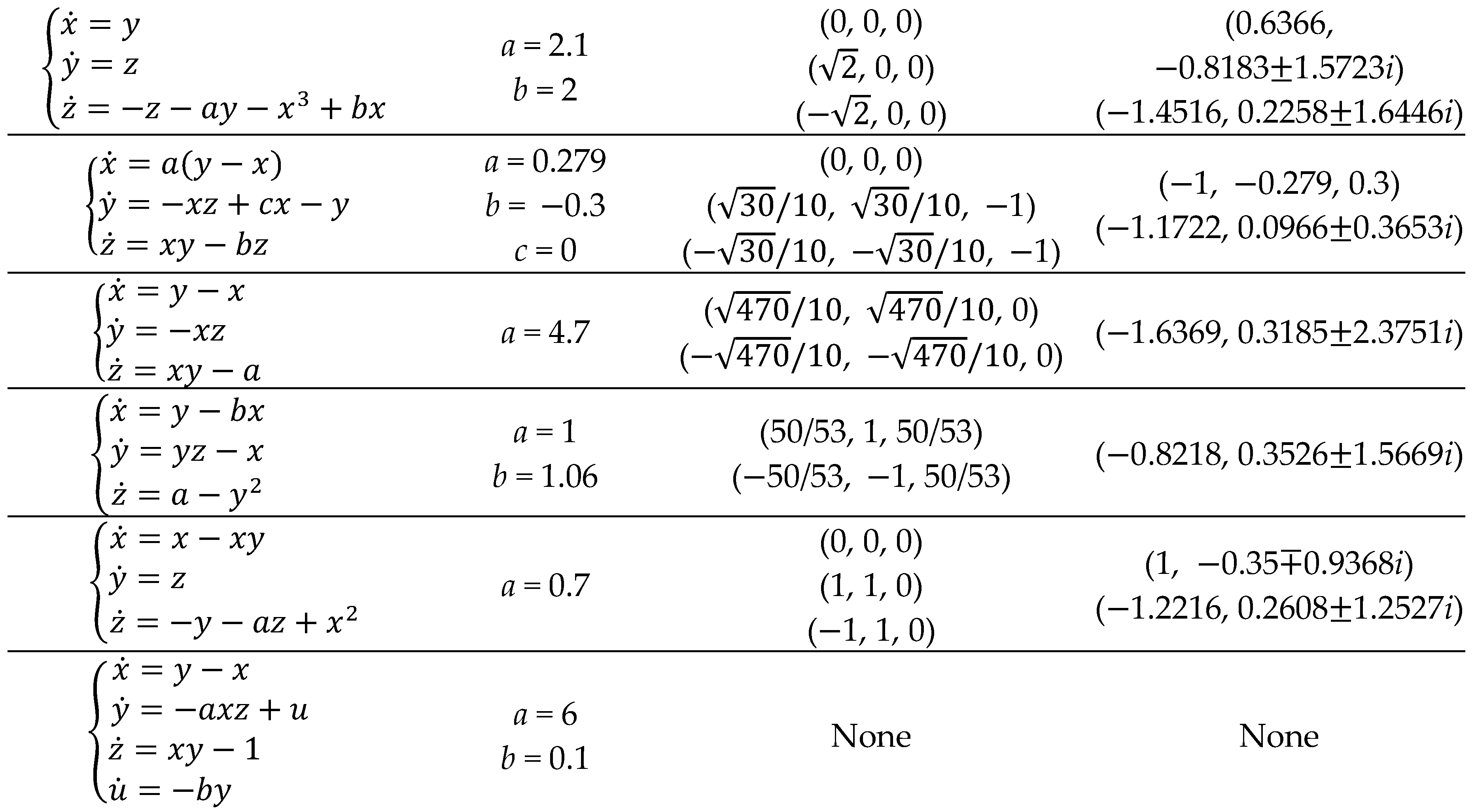 | |||
Sometime, even the chaotic system has no equilibrium point, the system still can exhibit symmetric pairs of coexisting attractors, in which case, all the attractors are named as the type of hidden attractor [26]. One example is the simple seven-term system with two quadratic nonlinearities,
which is exactly the diffusion less Lorenz system with an added variable u. The coefficients of five of the seven terms can be normalized to ±1 through a linear rescaling of the four variables and time without loss of generality, system (1) is completely described by only two independent parameters, taken here as a and b. Although the system (4) has no equilibrium point, system (4) can still give chaotic or even hyperchaotic solutions [27]. For example, when a = 6, b = 0.1, a quasi-periodic torus coexists with a symmetric pair of chaotic attractors, as shown in Figure 10.
3. Offset boosting for symmetric pairs of strange attractors
If a variable substitution: , (here ,) in a dynamical system ( leads to (, the variable in system obtains the operation of offset boosting, and for this reason its average value gets boosted by the new introduced constant . The variable can be a signal in an electrical system, correspondingly the signal gets offset-boosted by a direct current voltage of . When the operation only introduces an independent constant in one dimension in the system, then the system was named as a variable-boostable system [28]. For a variable-boostable dynamical system (, there exists one and only one () satisfying, where k is a nonzero constant.
Offset boosting is an effective technique for shifting an attractor in phase space without changing the basic dynamics of a system. In a system , , take the substitution of , , , the offset of the variable get boosted. The offset parameter can move the attractor switching from the negative zone to the positive zone divided by the dimension , . In fact, an attractor can be moved in any dimension by offset boosting. From this view, when the offset boosting is completed by an absolute-value function, corresponding attractors can get doubled by the combination of polarity compensation. The mechanism is as explained in [29,30,31].
For a dynamical system,
If the system (5) has coexisting solutions identified by attractors like, , take the offset-boosting constants as , subjecting to any state vector to satisfy , then substituting with, into system (5) like,
Then:
(I) System (6) is of symmetry according to the dimension of ;
(II) System (6) has 2m coexisting attractors;
(III) All the attractors in system (6) share the same structure with the ones in system (5) and all the equilibria in system (6) have the same stabilities with those of system (5).
Take the above method for constructing coexisting attractors in the Rössler system [32,33], which is described by,
We know, when a = b = 0.2, c = 5.7, the system is chaotic with Lyapunov exponents (LEs) of (0.0714, 0, −5.3943) and a Kaplan-Yorke dimension of DKY = 2.0132. Replace the variable z with an absolute function |z|− d,
This time, system (8) turns to be a reflection invariant system since it is of polarity balance when z turns to be –z, and the attractors get doubled according to the z-axis, as shown in Figure 11. Larger offset constant d will separate the coexisting attractors more far away in this direction, for example, let d = 12, the two attractors stand in phase space far away, as shown in Figure 12. More absolute functions can turn the original Rössler system to be of other regimes of symmetry. That is to say, take |x| – d1, |y| – d2, |z| – d3, the derived system is of inversion symmetry, and when the variables x, y, and z get polarities inversed, the derived system keep the same equation, as written in system (9),
And at this time, the original attractor gets three times of doubling, and then totally eight attractors show up, as displayed in Figure 13.
4. Coexisting strange attractors of conditional symmetry
As we know, a system variable like x can be written as x = |x|sgn(x). In fact, any variable in an equation includes two types of inherent features: the amplitude and the polarity of the variable. Therefore, there are two effective polarity adapters: one is the signum function for maintaining the polarity, and the other is the absolute value function removing the polarity. The combination of signum function and absolute-value function can producing coexisting doubled attractors. At the same time, the absolute-value function is an effective way for the producing of functional polarity reverse leading to coexisting conditional symmetric attractors. Therefore, from the conception of conditional symmetry, we could conclude that if some of the variables get the polarities reversed, the additional operation like offset boosting may return the polarity balance and result in symmetrically attractor doubling or conditional symmetry, as shown in Figure 14. The polarity adapter and slide polarity converter are widely applied in a dynamical system for giving conditional symmetry or attractor self-reproducing.
For a dynamical system (, when the variable substitution including polarity reversal and offset boosting such as , (here ,, and are not identical, ) lead to the derived system retaining its polarity balance and satisfy ( he system ( is of l-dimensionally conditional symmetry since the polarity balance needs an l-dimensional offset boosting [34,35,36,37,38,39,40,41,42]. For a three-dimensional system, (, the regime could be conditional rotational symmetry in 1-dimension and conditional reflection symmetry in 1-dimension or 2-dimension.
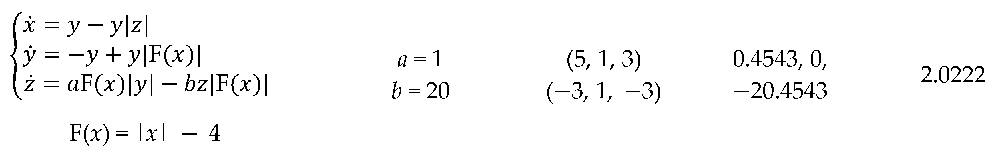
The mechanism of conditional symmetry is associated with the offset boosting for polarity balance. Suppose we want to construct a conditional reflection symmetric system, here the variable gets polarity reversed, which will revise the polarity of , and in turn requires the polarity reverse on the right-hand side of to get without influencing any of the other dimensions for polarity balance. Aim to this end, based on exhaustive researching, a chaotic system of conditional reflection symmetry was found as shown,
When z gets the polarity reversed, the polarity of the last dimension is destroyed unless the function F(x) = |x|−3 get a reversed polarity to recover this balance. The polarity reverse of F(x) is induced by the offset boosting of x, that is to say, when x → x + d, the first two dimensions do not change, but the function F(x+d) turns to be −F(x) since the absolute-value function has two reverse slopes during different position of its variable. The newly balanced polarity brings a pair of coexisting attractors across the x and z-axis in phase space, as shown in Figure 15. We see that the direction of the attractor in the dimension of x does not change but the direction in the dimension of x does be overturned. Therefore, we can call this polarity balance as ‘one-jump polarity balance’.
The ‘one-jump polarity balance’ can also happens in those rotational symmetric systems. As to system (11), here the polarity reverse in the dimension y and z breaks the polarity balance in the last dimension until the offset boosting of x returns its balance without destroy the first dimension since adding a constant term does not change the value of the derivative. As shown in Figure 16, this time the direction of coexisting attractors does not change in the x-axis, but change both in the y and z dimension.
Sometimes, more operations of offset boosting are needed for balancing the polarity reverse of some of the variables. At this time, the conditional symmetry could be of ‘two-jump polarity balance’ or ‘more-jump polarity balance’. Like the system (12), here polarity reverse of z is washed out by the offset boosting in the dimensions of x and y. This time, we can see that direction of the coexisting attractors does not change in the x and y dimension, but turn down in the z-axis, as shown in Figure 17. The ‘two-jump polarity balance’ may also happens in the same dimension and leave more variables for polarity reverse, as displayed in the system (13), here two variables get polarity reversed like x and y, but the polarity balance is returned by the offset boosting in the z-dimension. The coexisting attractors, shown in Figure 18, compared with those of system (12), system (13) has coexisting attractors with opposite directions in the dimension of x and y, but with the same direction in the z-dimension.
More operations of offset boosting from the absolute-value functions could be introduced for recovering the polarity balance, such as in system (14), which contains six absolute-value functions for balancing the polarity reverse of the variable x. As shown in Figure 19, here the direction of the coexisting attractors in x-dimension gets reversed, but does not change in the y and z dimension except the two-dimensional offset boosting. More interestingly, sometimes conditional symmetry may happen in symmetric systems. In this case, the offset boosting of some of the system variables also may return other types of conditional symmetry. As we know, the original version of system (15) is the simplified Lorenz system, but the two-dimensional offset boosting with y and z returns a conditional reflection symmetry, as shown in Figure 20. Note that, it is interesting that system (5) is an asymmetric system now, although it has symmetric attractors in a conditional symmetric way, which means an asymmetric system may hosting symmetric attractors.
Many candidates of chaotic systems with coexisting attractors have been explored based on various system structures, such as those of chaotic system with hidden attractors [40], those symmetric systems [35,36,37,38,39,40,41], as listed in Table. 2. Those system could be of symmetry, or asymmetry, or jerk system. Readers could check these systems to see if they are of polarity balance. Here the factors for polarity balance are from the system variables and also recovered by the absolute functions. The polarity broken is originated from the polarity reverse of some of the system variables, and the polarity balance is reconstructed by the internal polarity reverses of the absolute-value function. One absolute-value function introduces one time of polarity reverse by the offset boosting; multiple absolute-value functions drive multiple times of polarity jump of offset boosting. Those chaotic systems with amplitude control [43] or other coexisting attractors [44] may preserve this property since the polarity reverse induced by the offset boosting does not fundamentally change the system structure.
| Equations | Parameters | (x0, y0, z0) | LEs | DKY |
|---|---|---|---|---|
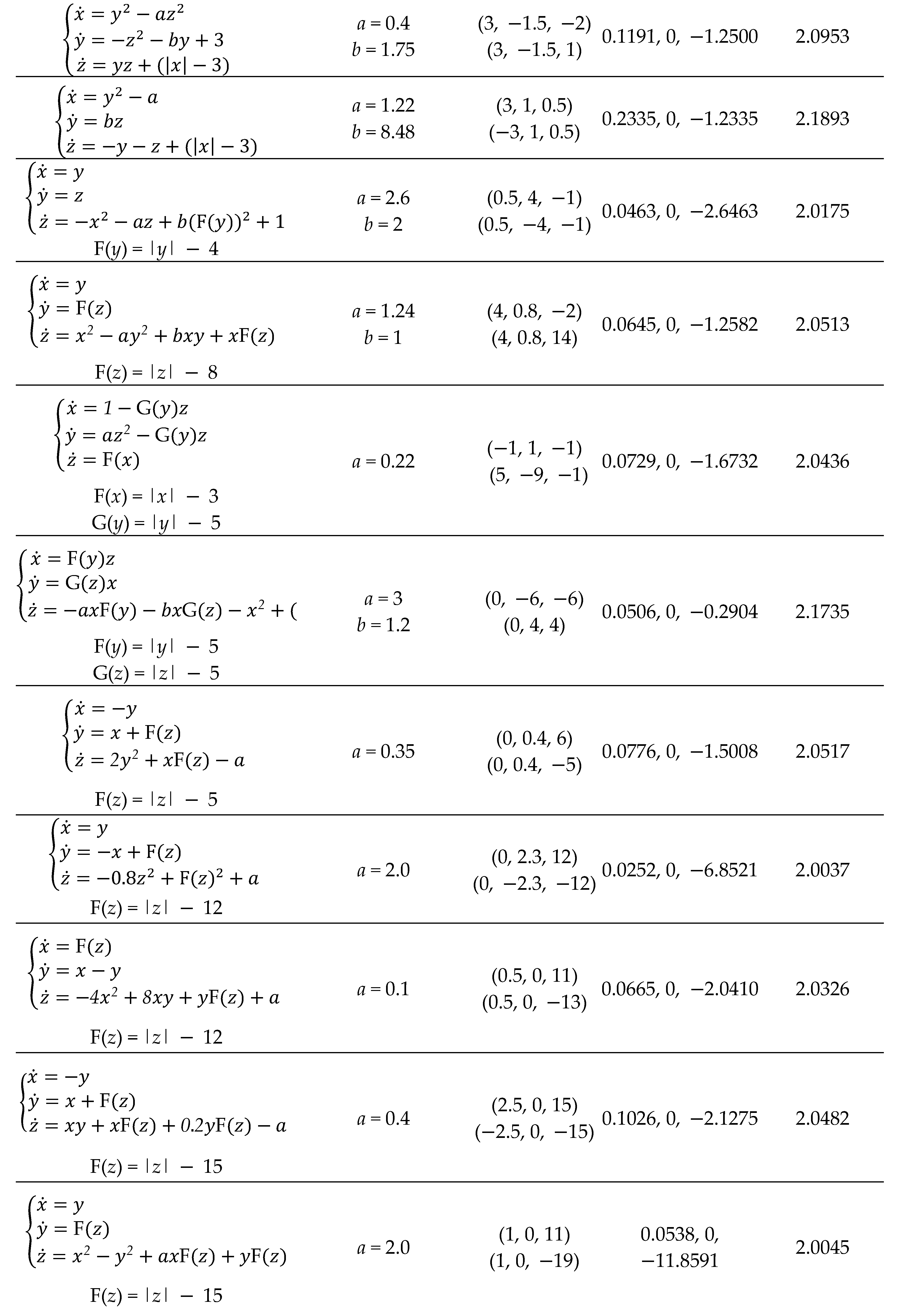 | ||||
 | ||||
 | ||||
 | ||||
From this view, the route for conditional symmetry is just drawing support from offset boosting to balance the destroyed polarity. The absolute value is just a polarity carrier for returning the polarity balance. The conditional symmetry is in fact a specific attractor rotation of offset dependence [45] without rotation matrix, where conditional reflectional symmetry could be regarded as the attractor rotation of one-dimensional 180 degrees, namely antiphase rotation (could be regarded as from the first quadrant to the second quadrant); meanwhile the conditional rotational symmetry could be regarded as the attractor rotation of two-dimensional 135 degrees, namely anti-quadrant rotation (could be regarded as from the first quadrant to the third quadrant in a two-dimensional plane). In fact, more generally, the polarity balance may be recovered from any combinations of variable and its offset boosting. We can also conclude that even a 3D chaotic system of inversion symmetry can recover its polarity balance based on offset boosting, and such an additional selection of polarity balance can also be employed for repellor construction [34]. As displayed in system TCSS6,
The offset boosting of the variables x, y, and z introduces polarity reverse for balancing the polarity destroyed from the variable of t, and thus returning coexisting repellors, as shown in Figure 21, here various operations of offset boosting of the variables return two repellors with conditional symmetry to the coexisting attractors.
The offset boosting within a trigonometric function, such as sinusoidal function or tangent function, can also balance the polarity reverse [46] and thus reproducing infinitely many coexisting attractors of conditional symmetry [39]. As appears in system (17),
Here the sinusoidal function of x also brings a new polarity reverse and return the polarity balance in the last dimension of system (17), and thus introducing more coexisting attractors based on periodic offset boosting, as shown in Figure 22. The flexible combinations of offset-boosting-oriented polarity reverse and variable polarity reverse lead to abundant candidates of chaotic systems with infinitely many coexisting attractors or repellors [47].
5. Symmetry and elegance in simple chaotic circuits
Furthermore, symmetry and conditional symmetry can be seen in the circuits. As we know, the restriction of voltage and current in a circuit is under the rule governed by the structure of circuit topology, and the individual characteristic of a circuit component. The structure of circuit topology gives the macro-restriction with the voltage and current, while the individual characteristic of a circuit component leads to a local micro-restriction. The former corresponds to the circuit law of Kirchhoff law, and the later is related the local restriction from a circuit element. All the circuit variables must obey the two types of constraints, but we still see that the constraint from the local component endows the flexibility in voltage and current values. Therefore, I call these two constraints with a Chinese Ancient philosophy vocabulary as ‘a square earth with a round sky above’, as shown in Figure 23. The concept of ‘a square earth with a round sky above’ is the philosophical idea in ancient China, which is a manifestation of the theory of ‘Yin and Yang’. The sky and circle symbolize movement, but the earth and square represent stillness. In fact, the combination shows a balance of ‘yin and yang’ with the complementary movement and stillness. The concept of ‘round sky and square earth’ has been shown in ancient Chinese architecture, currency and other aspects, such as the Temple of Heaven, square hole coins and other patterns and structures.
Moreover, in circuit, there are many cases of symmetry and duality. We can enumerate many circuit structures and corresponding circuit laws, such as capacitive and inductive components, voltage source and current source, series for voltage and parallel for current, series resonance and parallel resonance, time constant of resistor and capacitor and the time constant of conduction and inductance. Typically, many circuits of series structure could be transformed to be of parallel structure and give symmetric attractors or coexisting attractors of conditional symmetry. As shown Figure 24, the simple series circuit [48] including an inductor, a capacitor and a memristor can produce symmetric chaotic attractor, as show in Figure 25. The circuit realizes the equation of system (18) with rotational symmetry according to the variables y and z.
Conditional symmetry of coexisting attractors can also be generated in a simple parallel circuit structure [49]. The chaotic system (19),
has coexisting chaotic attractors of rotational conditional symmetry when a = 0.6, b = 1, c = 2, as displayed in Figure 26. The structure of system (19) is unique, and can be implemented based on a parallel circuit with a capacitor, a resistor, and an meminductor, as shown in Figure 27. This simple structure also oscillates outputting two coexisting attractors, as shown in Figure 28. We can declare that people can realize these systems with a dual circuit structure if they want to switch the circuit between the series and parallel.
In fact, the elegant structure or symmetric property of a system does not indicate its simple or easy structure. For example, for doubling the coexisting attractors [28,29,30], let’s see the system (20),
the coexisting attractors locate in phase space according to the axis of symmetry x = 0. Here the constant d modifies the distance between two coexisting symmetric attractors, when it increases from d = 4.11 to be d = 8, the distance between those symmetric attractors gets increased also, as shown in Figure 29 and Figure 30. Here the chaotic phase trajectories are elegant and simple, but the circuit for realizing them is not simple, typically it is realized based on three lines of operational-amplifier-based integral structure [27], [50].
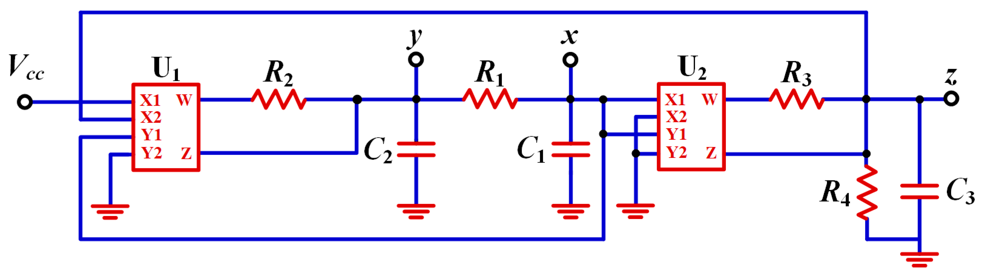
For many of those symmetric chaotic systems, the simple circuit could be constructed by utilizing the inherent characteristics of a multiplier and the differential constraint of the capacitor [51]. As we know, the multiplier AD633 can convert voltage to current by an external resistor. The external voltage transformation characteristic of AD633 obeys the relationship of . If a resistor connects the output point W and Z in series, as shown in Figure 31(a), the output current satisfies 0 and for a large input resistor of the Z port with a small input current. Thus, the output voltage satisfies the balance of current: . Consequently, the current associated with AD633 subject to . Various combinations of inputs realize those terms with different degrees according to the input variable, and therefore, a multiplier provides the linear terms and quadratic terms for circuit calculation. Furthermore, the connection of resistor and capacitor drives flexible integration calculation. When two capacitors are coupled with a resistor as shown in Figure 31(b), the current identified by equals the current through the capacitor resulting in, and similarly leads to the symmetric restraint like . When a capacitor and a resistor connect in parallel, the current equation is . From the above two class of basic circuit constraints, many symmetric chaotic systems with quadratic terms could be implemented in an easy way. Like the system, written as,
it can be realized with a compact structure, as shown in Figure 32.
6. Conclusion
In physical world, there are many symmetric systems keeping their stability against the revise of polarity from some of the dimensions. Symmetric systems provide symmetric solutions, and even when the symmetry is broken, the symmetry turns to be accompanied by the coexisting symmetric pairs of attractors. The polarity revise can resort to those direct polarity reverses from some of the system variables, or is derived by offset boosting with any of the variables. Therefore, symmetric system can be reconstructed by introducing an absolute-value function and a signum function. More widely, the offset boosting can also be employed for rebuilding the chaotic system with conditional symmetry. The structure of a system is not necessarily related with symmetric or elegant circuit structure. Simple or elegant circuit structure depends on the cute combinations of modern circuit component.
Author Contributions
Conceptualization, C.L.; data curation, C.L. and Z.L.; funding acquisition, C.L.; investigation, C.L. and Y.J.; methodology, C.L.; project administration, T.L.; resources, X.W.; software, C.L., Z.L. and Y.J.; supervision, T.L.; validation, X.W.; writing—original draft, C.L.; writing—review and editing, C.L. All authors have read and agreed to the published version of the manuscript.
Funding
This work was supported financially by the National Natural Science Foundation of China (Grant No.: 61871230), and a project on the reform of graduate education and Jiangsu graduate degree (Grant No.: JGKT23_C024).
Data Availability Statement
The data that support the findings of this study are available from the corresponding author upon reasonable request.
Conflicts of Interest
We declare that we have no known competing financial interest or personal relationship that could have appeared to influence the work reported in this paper.
References
- Lorenz, E. N. Deterministic nonperiodic flow. Journal of atmospheric sciences 1963, 20, 130–141. [Google Scholar] [CrossRef]
- Chen, G.; Ueta, T. Yet another chaotic attractor. Int. J. Bifurcat. Chaos 1999, 9, 1465–1466. [Google Scholar] [CrossRef]
- Chua, L. E. O. N. O.; Komuro, M.; Matsumoto, T. The double scroll family. IEEE transactions on circuits and systems 1986, 33, 1072–1118. [Google Scholar] [CrossRef]
- Ali, A. M.; Ramadhan, S. M.; Tahir, F. R. A Novel 2D—Grid of Scroll Chaotic Attractor Generated by CNN. Symmetry 2019, 11, 99. [Google Scholar] [CrossRef]
- Brisson, G. F.; Gartz, K. M.; McCune, B. J.; O'Brien, K. P.; Reiter, C. A. Symmetric attractors in three-dimensional space. Chaos Solit Fractals 1996, 7, 1033–1051. [Google Scholar] [CrossRef]
- Li, C.; Sun, J.; Lu, T.; Lei, T. Symmetry evolution in chaotic system. Symmetry 2020, 12, 574. [Google Scholar] [CrossRef]
- Vidal, G.; Mancini, H. Hyperchaotic synchronization under square symmetry. Int. J. Bifurcat. Chaos 2009, 19, 719–726. [Google Scholar] [CrossRef]
- Hu, W.; Liu, T.; Han, Z. Dynamical Symmetry Breaking of Infinite-Dimensional Stochastic System. Symmetry 2022, 14, 1627. [Google Scholar] [CrossRef]
- Ramamoorthy, R.; Rajagopal, K.; Leutcho, G. D.; Krejcar, O.; Namazi, H.; Hussain, I. Multistable dynamics and control of a new 4D memristive chaotic Sprott B system. Chaos Solit Fractals 2022, 156, 111834. [Google Scholar] [CrossRef]
- Kamdjeu Kengne, L.; Kamdem Tagne, H. T.; Kengnou Telem, A. N.; Mboupda Pone, J. R.; Kengne, J. A broken symmetry approach for the modeling and analysis of antiparallel diodes-based chaotic circuits: a case study. Analog Integrated Circuits and Signal Processing 2020, 104, 205–227. [Google Scholar] [CrossRef]
- Bloch, A. M.; Krishnaprasad, P. S.; Marsden, J. E.; Murray, R. M. Nonholonomic mechanical systems with symmetry. Archive for rational mechanics and analysis 1996, 136, 21–99. [Google Scholar] [CrossRef]
- Olfati-Saber, R. Normal forms for underactuated mechanical systems with symmetry. IEEE Transactions on automatic control 2002 47, 305–308. [CrossRef]
- Leonard, N. E.; Marsden, J. E. Stability and drift of underwater vehicle dynamics: mechanical systems with rigid motion symmetry. Physica D: Nonlinear Phenomena 1997, 105, 130–162. [Google Scholar] [CrossRef]
- Mory, J. F. Oil prices and economic activity: is the relationship symmetric? The Energy Journal 1993, 14, 151–161. [Google Scholar] [CrossRef]
- Bischi, G. I.; Gallegati, M.; Naimzada, A. Symmetry-breaking bifurcations and representativefirm in dynamic duopoly games. Annals of Operations Research 1999, 89, 252–271. [Google Scholar] [CrossRef]
- Kondepudi, D. K.; Nelson, G. W. Chiral-symmetry-breaking states and their sensitivity in nonequilibrium chemical systems. Physica A: Statistical Mechanics and its Applications 1984, 125, 465–496. [Google Scholar] [CrossRef]
- Piñeros, W. D.; Tlusty, T. Spontaneous chiral symmetry breaking in a random driven chemical system. Nature Communications, 2022, 13, 2244. [Google Scholar] [CrossRef] [PubMed]
- Kondepudi, D. K.; Nelson, G. W. Chiral symmetry breaking in nonequilibrium chemical systems: time scales for chiral selection. Physics Letters A 1984, 106, 203–206. [Google Scholar] [CrossRef]
- Amit, D. J.; Tsodyks, M. V. Quantitative study of attractor neural networks retrieving at low spike rates: II. Low-rate retrieval in symmetric networks. Network: Computation in Neural Systems 1991, 2, 275–294. [Google Scholar] [CrossRef]
- Cho, M. W.; Chun, M. Y. Two symmetry-breaking mechanisms for the development of orientation selectivity in a neural system. Journal of the Korean Physical Society 2015, 67, 1661–1666. [Google Scholar] [CrossRef]
- Turvey, M. T.; Shaw, R. E. Ecological foundations of cognition. I: Symmetry and specificity of animal-environment systems. Journal of Consciousness Studies 1999, 6, 95–110. [Google Scholar]
- Persson, L.; de Roos, A. M. Symmetry breaking in ecological systems through different energy efficiencies of juveniles and adults. Ecology 2013, 94, 1487–1498. [Google Scholar] [CrossRef] [PubMed]
- Dunitz, J. D.; Orgel, L. E. Electronic properties of transition-metal oxides—I: Distortions from cubic symmetry. Journal of Physics and Chemistry of Solids 1957, 3, 20–29. [Google Scholar] [CrossRef]
- Berg, R. A.; Wharton, L.; Klemperer, W.; Büchler, A.; Stauffer, J. L. Determination of electronic symmetry by electric deflection: LiO and LaO. The Journal of Chemical Physics 1965, 43, 2416–2421. [Google Scholar] [CrossRef]
- Sprott, J. C. Simplest chaotic flows with involutional symmetries. Int. J. Bifurcat. Chaos 2014, 24, 1450009. [Google Scholar] [CrossRef]
- Li, C.; Sprott, J. C. Coexisting hidden attractors in a 4-D simplified Lorenz system. Int. J. Bifurcat. Chaos 2014, 24, 1450034. [Google Scholar] [CrossRef]
- Li, C.; Sprott, J. C.; Thio, W.; Zhu, H. A new piecewise linear hyperchaotic circuit. IEEE Transactions on Circuits and Systems II: Express Briefs 2014, 61, 977–981. [Google Scholar] [CrossRef]
- Li, C.; Sprott, J. C. Variable-boostable chaotic flows. Optik 2016, 127, 10389–10398. [Google Scholar] [CrossRef]
- Li, C.; Wang, R.; Ma, X.; Jiang, Y.; Liu, Z. Embedding any desired number of coexisting attractors in memristive system. Chinese Physics B 2021, 30, 120511. [Google Scholar] [CrossRef]
- Li, C.; Lu, T.; Chen, G.; Xing, H. Doubling the coexisting attractors. Chaos 2019, 29, 051102. [Google Scholar] [CrossRef]
- Wang, R.; Li, C.; Kong, S.; Jiang, Y.; Lei, T. A 3D memristive chaotic system with conditional symmetry. Chaos Solit Fractals 2022, 158, 111992. [Google Scholar] [CrossRef]
- Rössler, O. E. An equation for continuous chaos. Physics Letters A 1976, 57, 397–398. [Google Scholar] [CrossRef]
- Li, C.; Hu, W.; Sprott, J. C.; Wang, X. Multistability in symmetric chaotic systems. Eur. Phys. J-Spec. T 2015, 224, 1493–1506. [Google Scholar] [CrossRef]
- Li, C.; Sprott, J. C.; Liu, Y. Time-reversible chaotic system with conditional symmetry. Int. J. Bifurcat. Chaos 2020, 30, 2050067. [Google Scholar] [CrossRef]
- Gu, Z.; Li, C.; Iu, H. H.; Min, F.; Zhao, Y. Constructing hyperchaotic attractors of conditional symmetry. Eur. Phys. J. B 2019, 92, 1–9. [Google Scholar] [CrossRef]
- Lu, T.; Li, C.; Wang, X.; Tao, C.; Liu, Z. A memristive chaotic system with offset-boostable conditional symmetry. Eur. Phys. J-Spec. T 2020, 229, 1059–1069. [Google Scholar] [CrossRef]
- Li, C.; Sprott, J. C.; Xing, H. Constructing chaotic systems with conditional symmetry. Nonlinear Dynamics 2017, 87, 1351–1358. [Google Scholar] [CrossRef]
- Li, C.; Sprott, J. C.; Liu, Y.; Gu, Z.; Zhang, J. Offset boosting for breeding conditional symmetry. Int. J. Bifurcat. Chaos 2018, 28, 1850163. [Google Scholar] [CrossRef]
- Li, C.; Xu, Y.; Chen, G.; Liu, Y.; Zheng, J. Conditional symmetry: Bond for attractor growing. Nonlinear Dynamics 2019, 95, 1245–1256. [Google Scholar] [CrossRef]
- Li, C.; Sun, J.; Sprott, J. C.; Lei, T. Hidden attractors with conditional symmetry. Int. J. Bifurcat. Chaos 2020, 30, 2030042. [Google Scholar] [CrossRef]
- Li, C.; Sprott, J. C.; Zhang, X.; Chai, L.; Liu, Z. Constructing conditional symmetry in symmetric chaotic systems. Chaos Solit Fractals 2022, 155, 111723. [Google Scholar] [CrossRef]
- Zang, H.; Gu, Z.; Lei, T.; Li, C.; Jafari, S. Coexisting chaotic attractors in a memristive system and their amplitude control. Pramana 2020, 94, 62. [Google Scholar] [CrossRef]
- Gu, Z.; Li, C.; Pei, X.; Tao, C.; Liu, Z. A conditional symmetric memristive system with amplitude and frequency control. Eur. Phys. J-Spec. T 2020, 229, 1007–1019. [Google Scholar] [CrossRef]
- Gu, J.; Li, C.; Chen, Y.; Iu, H. H.; Lei, T. A conditional symmetric memristive system with infinitely many chaotic attractors. IEEE Access 2020, 8, 12394–12401. [Google Scholar] [CrossRef]
- Ma, X.; Li, C.; Li, Y.; Bi, L.; Qi, Z. Rotation control of an HR neuron with a locally active memristor. Eur. Phys. J. Plus 2022, 137, 542. [Google Scholar] [CrossRef]
- Li, C.; Sun, J.; Lu, T.; Sprott, J. C.; Liu, Z. Polarity balance for attractor self-reproducing. Chaos 2020, 30, 063144. [Google Scholar] [CrossRef] [PubMed]
- Li, C.; Gu, Z.; Liu, Z.; Jafari, S.; Kapitaniak, T. Constructing chaotic repellors. Chaos Solit Fractals 2021, 142, 110544. [Google Scholar] [CrossRef]
- Itoh, M.; Chua, L. O. Memristor hamiltonian circuits. Int. J. Bifurcat. Chaos 2011, 21, 2395–2425. [Google Scholar] [CrossRef]
- Jiang, Y.; Li, C.; Zhang, C.; Lei, T.; Jafari, S. Constructing meminductive chaotic oscillator. IEEE Transactions on Circuits and Systems II: Express Briefs, 2023.
- Zhang, X.; Li, C.; Dong, E.; Zhao, Y.; Liu, Z. A conservative memristive system with amplitude control and offset boosting. Int. J. Bifurcat. Chaos 2022, 32, 2250057. [Google Scholar] [CrossRef]
- Wu, J.; Li, C.; Ma, X.; Lei, T.; Chen, G. Simplification of chaotic circuits with quadratic nonlinearity. IEEE Transactions on Circuits and Systems II: Express Briefs 2021, 69, 1837–1841. [Google Scholar] [CrossRef]
- Piñeros, W. D., & Tlusty, T. (2022). Spontaneous chiral symmetry breaking in a random driven chemical system. Nature Communications, 13(1), 2244. [CrossRef]
Figure 1.
Symmetry, asymmetry and conditional symmetry in chaotic systems.
Figure 2.
Attractor of rotational symmetry in system (1) when σ = 0.279, r = 0, b = −0.3 and IC = (−0.1, 0.1, −2): (a) x−y, (b) x−z.
Figure 2.
Attractor of rotational symmetry in system (1) when σ = 0.279, r = 0, b = −0.3 and IC = (−0.1, 0.1, −2): (a) x−y, (b) x−z.
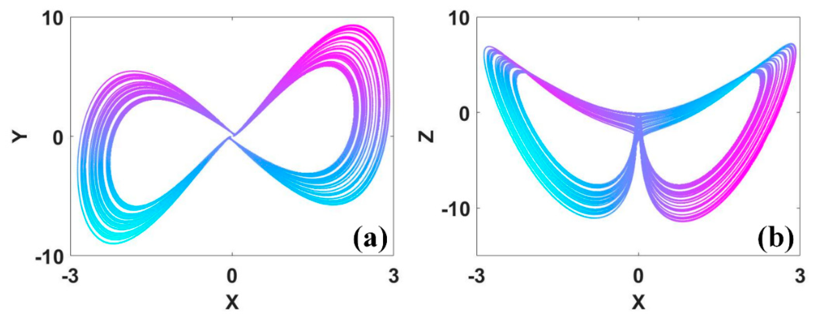
Figure 3.
Symmetric solutions under the broken symmetry.
Figure 4.
Symmetric pair of attractors with rotational symmetry in system (1) under the parameters σ = 0.256, r = 0, b = −0.3 and IC1 = (−0.1, 0.1, −2) (left), IC2 = (0.1, −0.1, −2) (right): (a) x−y, (b) x−z.
Figure 4.
Symmetric pair of attractors with rotational symmetry in system (1) under the parameters σ = 0.256, r = 0, b = −0.3 and IC1 = (−0.1, 0.1, −2) (left), IC2 = (0.1, −0.1, −2) (right): (a) x−y, (b) x−z.
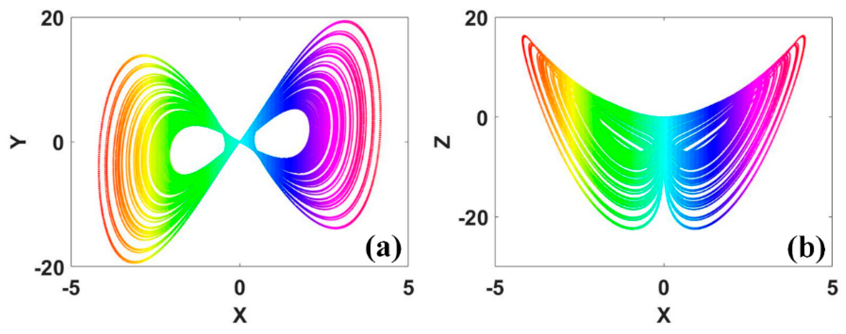
Figure 5.
Coexisting strange attractors of system (1) when σ = 0.279, r = 0, b = −0.3 and IC1 = (−0.1, 0.1, −2) (blue), IC2 = (−0.1, 0.1, −14) (cyan), IC3 = (0.1, −0.1, −14) (purple): (a) x−y, (b) x−z.
Figure 5.
Coexisting strange attractors of system (1) when σ = 0.279, r = 0, b = −0.3 and IC1 = (−0.1, 0.1, −2) (blue), IC2 = (−0.1, 0.1, −14) (cyan), IC3 = (0.1, −0.1, −14) (purple): (a) x−y, (b) x−z.
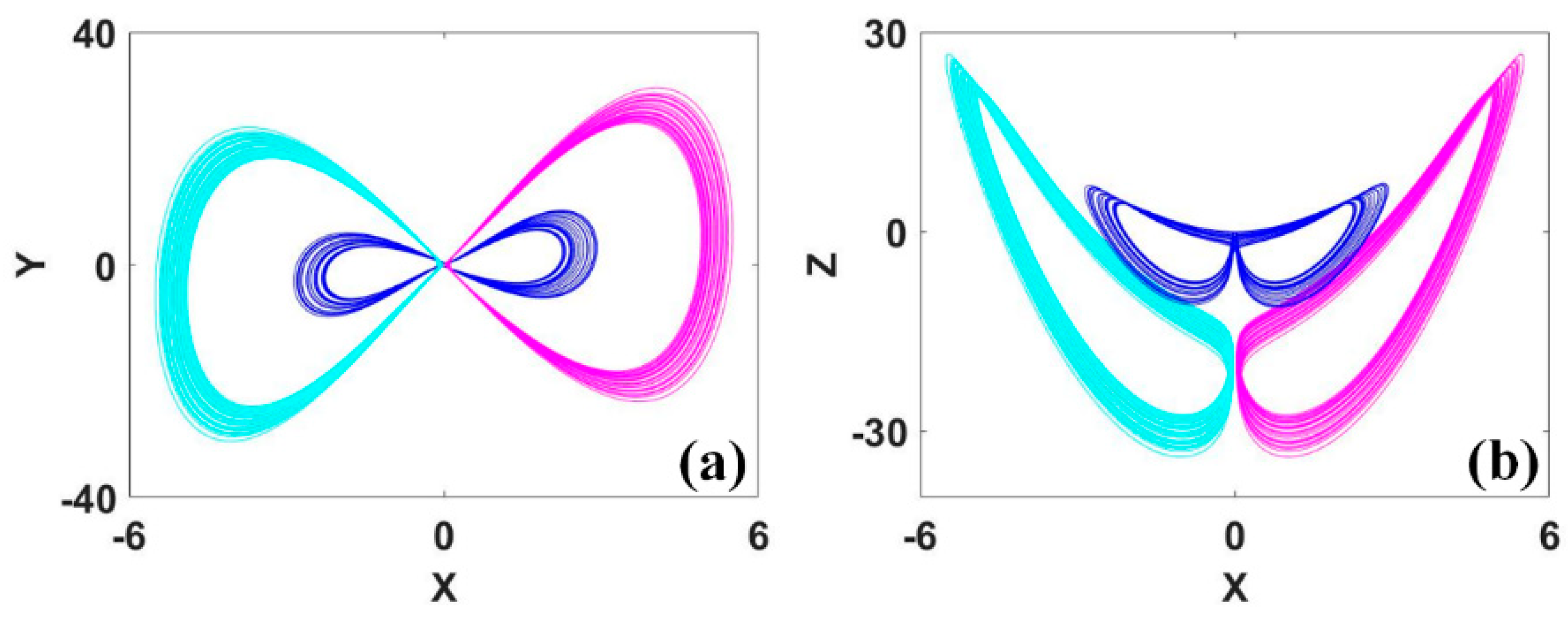
Figure 6.
Symmetric attractor of inversion symmetry in system (2) when a = 1.7, b = 2 and IC = (1, 0, 0): (a) x−y, (b) x−z.
Figure 6.
Symmetric attractor of inversion symmetry in system (2) when a = 1.7, b = 2 and IC = (1, 0, 0): (a) x−y, (b) x−z.
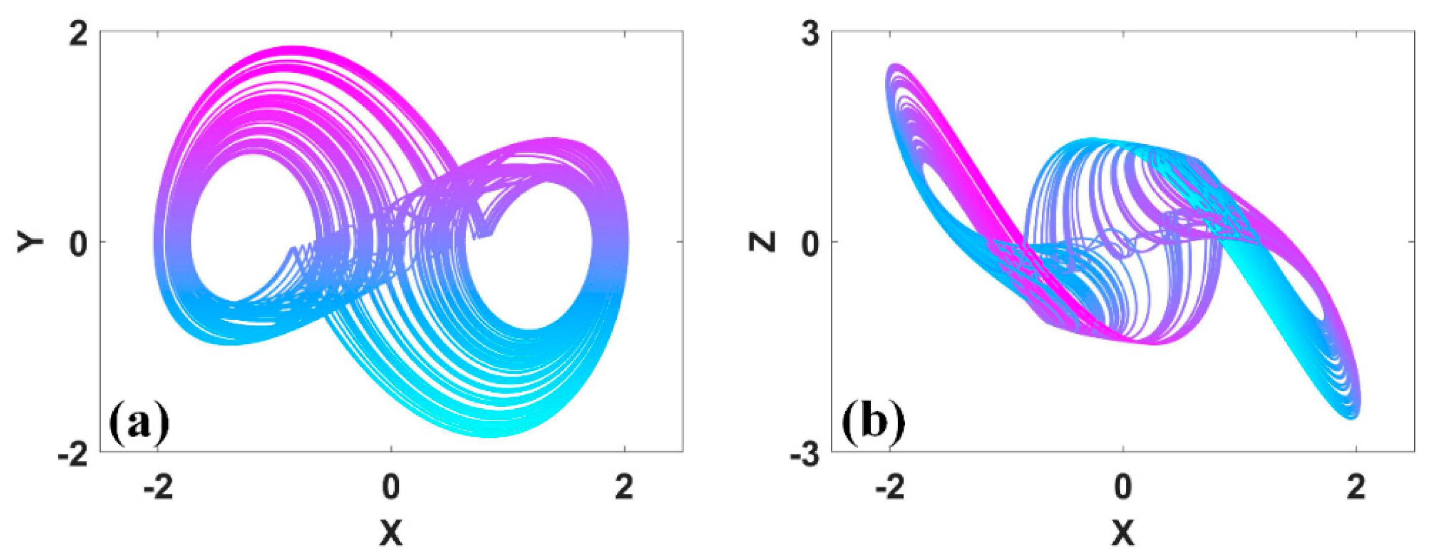
Figure 7.
A symmetric pair of coexisting attractors in system (2) when a = 2.1, b = 2 and IC1 = (−1, 0, 0) (left), IC2 = (1, 0, 0) (right): (a) x−y, (b) x−z.
Figure 7.
A symmetric pair of coexisting attractors in system (2) when a = 2.1, b = 2 and IC1 = (−1, 0, 0) (left), IC2 = (1, 0, 0) (right): (a) x−y, (b) x−z.
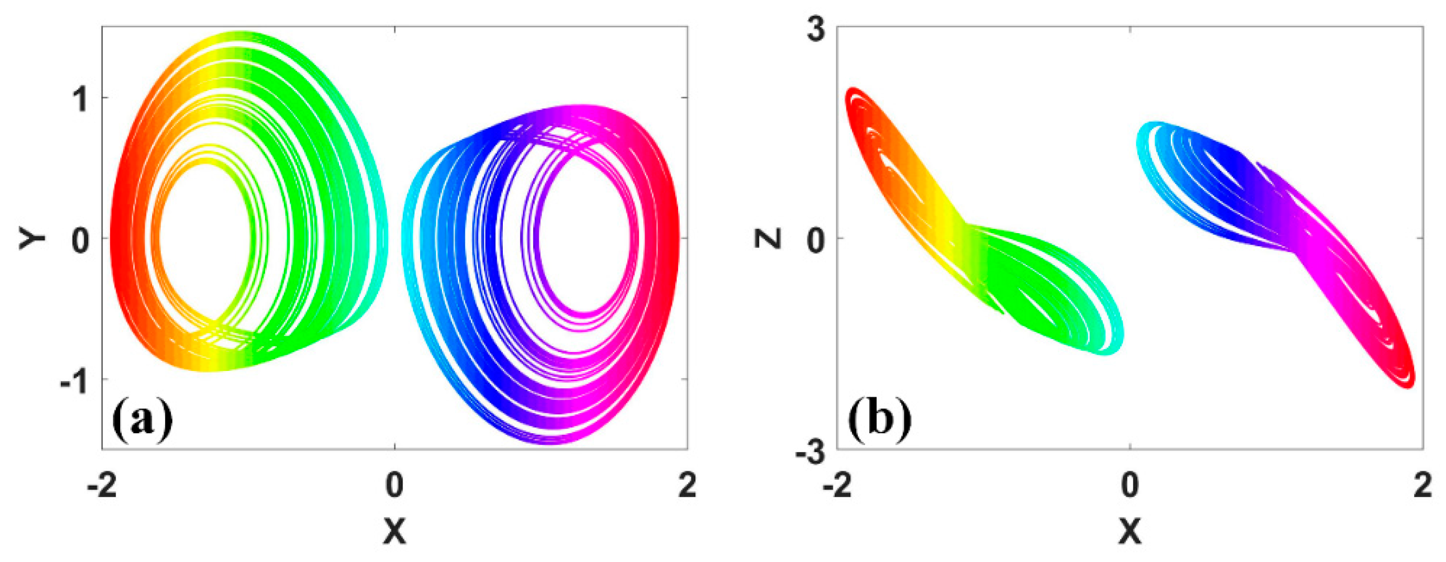
Figure 8.
Attractor of reflection invariant system (3) with a = 0.35 and IC = (−2, 2, 0): (a) x−y, (b) x−z.
Figure 8.
Attractor of reflection invariant system (3) with a = 0.35 and IC = (−2, 2, 0): (a) x−y, (b) x−z.
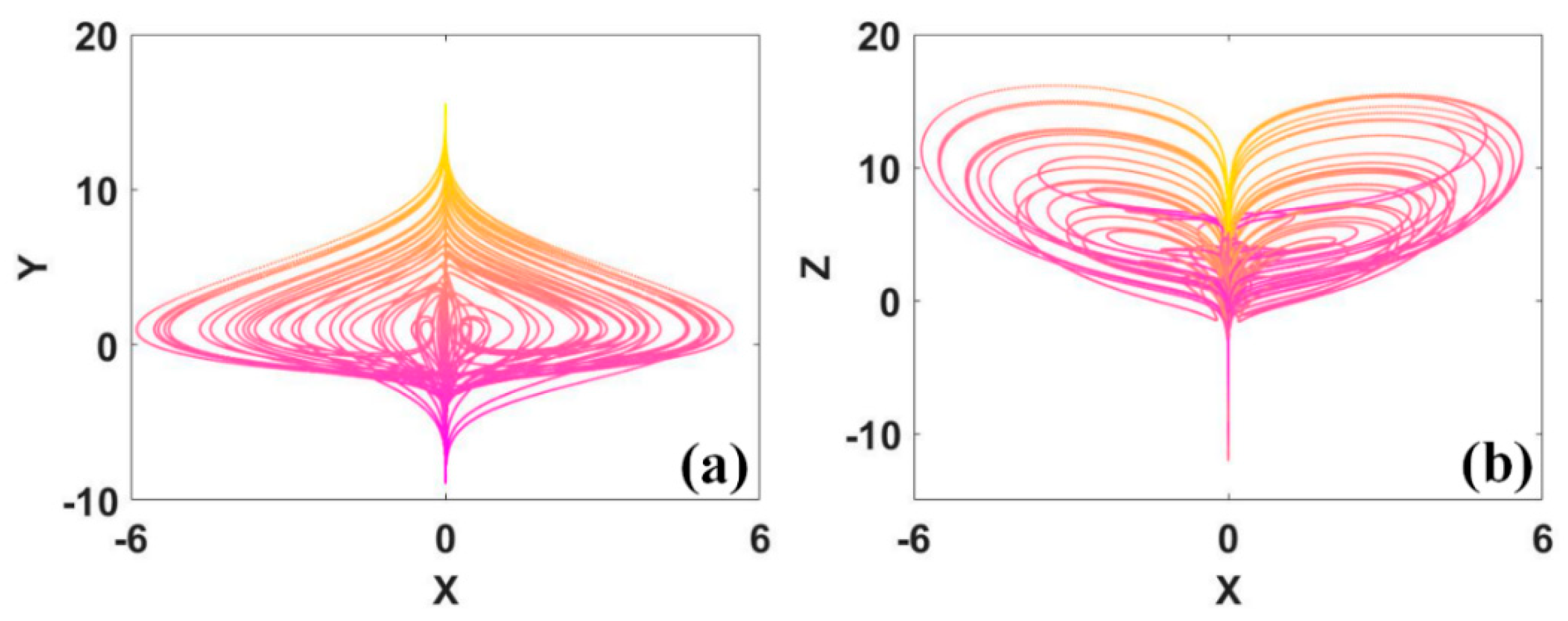
Figure 9.
A symmetric pair of attractors in reflection invariant system (3) with a = 0.7 and IC1 = (−2, 2, 0) (left), IC2 = (2, 2, 0) (right): (a) x−y, (b) x−z.
Figure 9.
A symmetric pair of attractors in reflection invariant system (3) with a = 0.7 and IC1 = (−2, 2, 0) (left), IC2 = (2, 2, 0) (right): (a) x−y, (b) x−z.
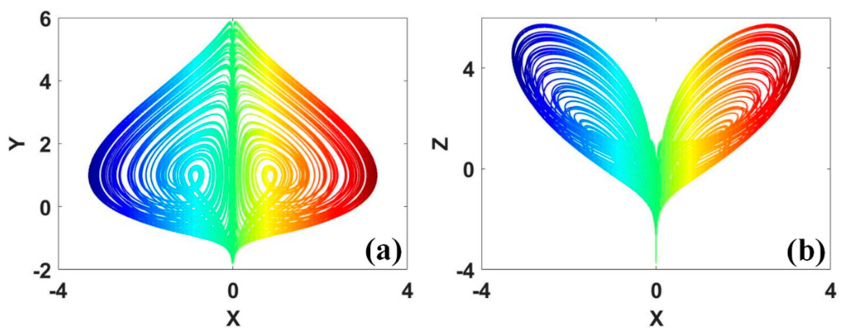
Figure 10.
Quasi-periodic torus coexisting with a symmetric pair of chaotic attractors at a = 6, b = 0.1 (red and blue attractors correspond to two symmetric initial conditions under IC = (0, ±4, 0, ∓5), cyan is for symmetric torus under IC = (1, −1, 1, −1)): (a) x-z, (b) y-z.
Figure 10.
Quasi-periodic torus coexisting with a symmetric pair of chaotic attractors at a = 6, b = 0.1 (red and blue attractors correspond to two symmetric initial conditions under IC = (0, ±4, 0, ∓5), cyan is for symmetric torus under IC = (1, −1, 1, −1)): (a) x-z, (b) y-z.
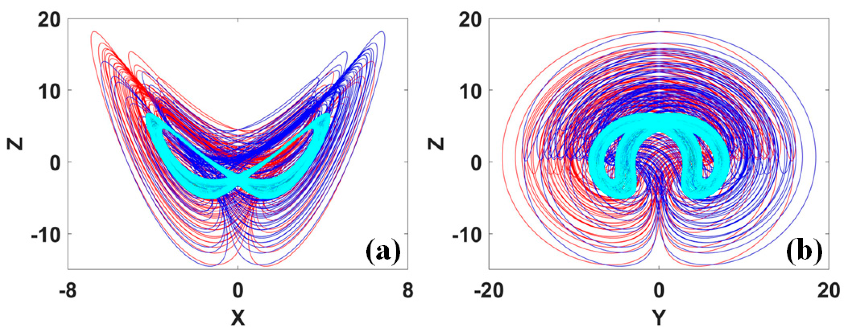
Figure 11.
Symmetric attractors of system (8) with a = b = 0.2, c = 6.5, d = 0 and IC1 = (−9, 0, 2) (up), IC2 = (−9, 0, −2) (down): (a) x−z, (b) y−z.
Figure 11.
Symmetric attractors of system (8) with a = b = 0.2, c = 6.5, d = 0 and IC1 = (−9, 0, 2) (up), IC2 = (−9, 0, −2) (down): (a) x−z, (b) y−z.
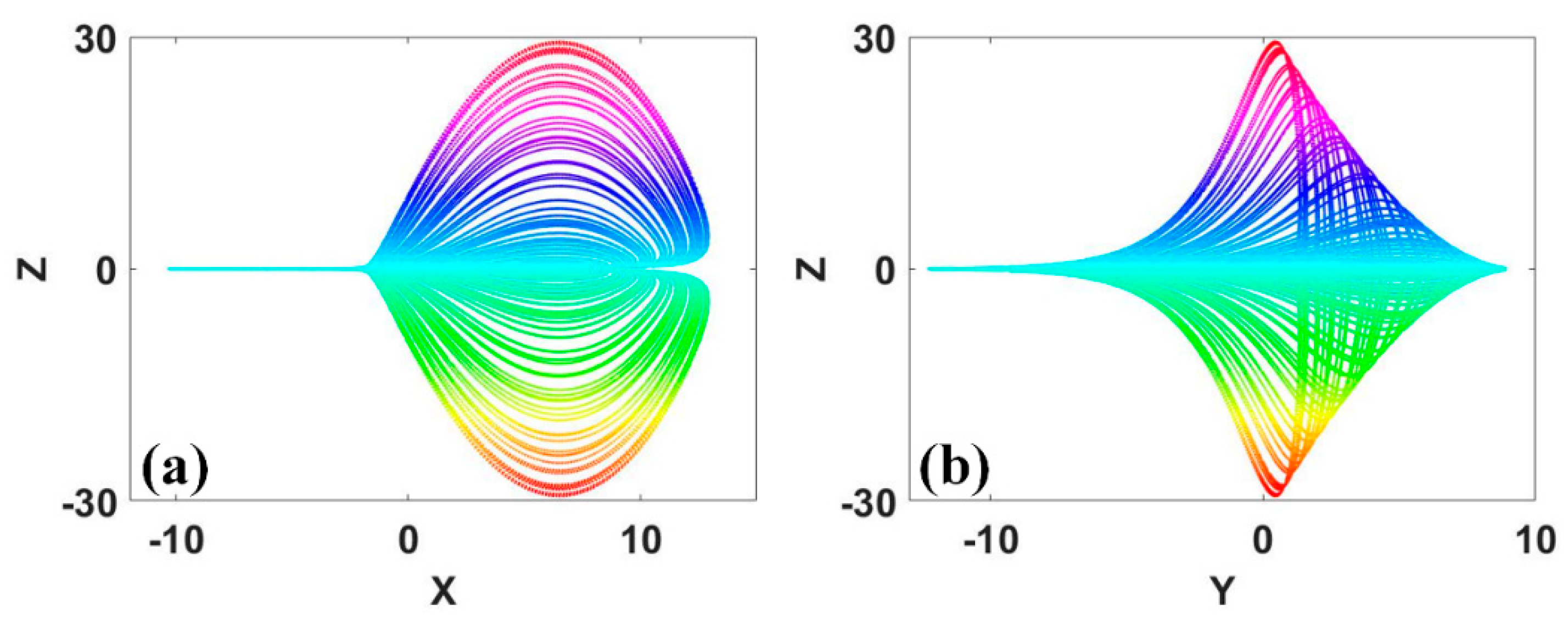
Figure 12.
Symmetric attractors of system (8) with a = b = 0.2, c = 6.5, d = 12 and IC1 = (−9, 0, 12) (up), IC2 = (−9, 0, −12) (down): (a) x−z, (b) y−z.
Figure 12.
Symmetric attractors of system (8) with a = b = 0.2, c = 6.5, d = 12 and IC1 = (−9, 0, 12) (up), IC2 = (−9, 0, −12) (down): (a) x−z, (b) y−z.
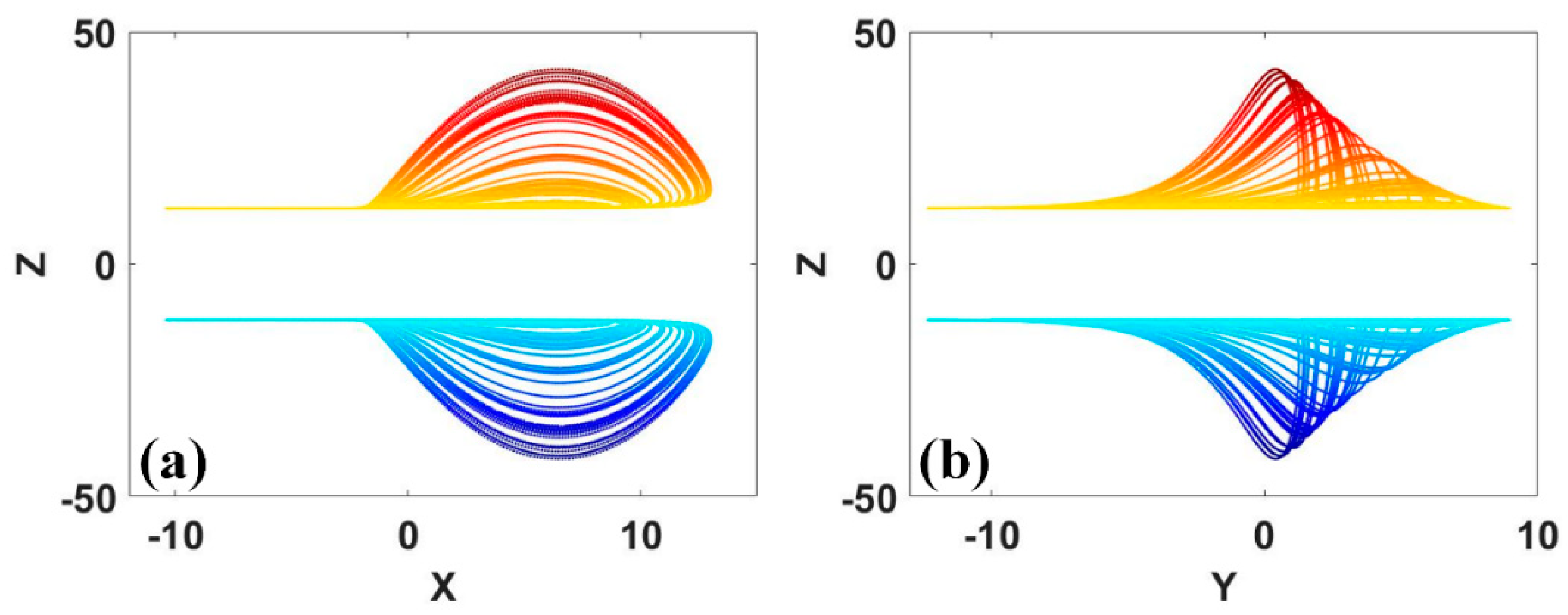
Figure 13.
Eight coexisting attractors of system (9) with a = b = 0.2, c = 6.5, d1 = 11, d2 = 13, d3 = 12.
Figure 13.
Eight coexisting attractors of system (9) with a = b = 0.2, c = 6.5, d1 = 11, d2 = 13, d3 = 12.
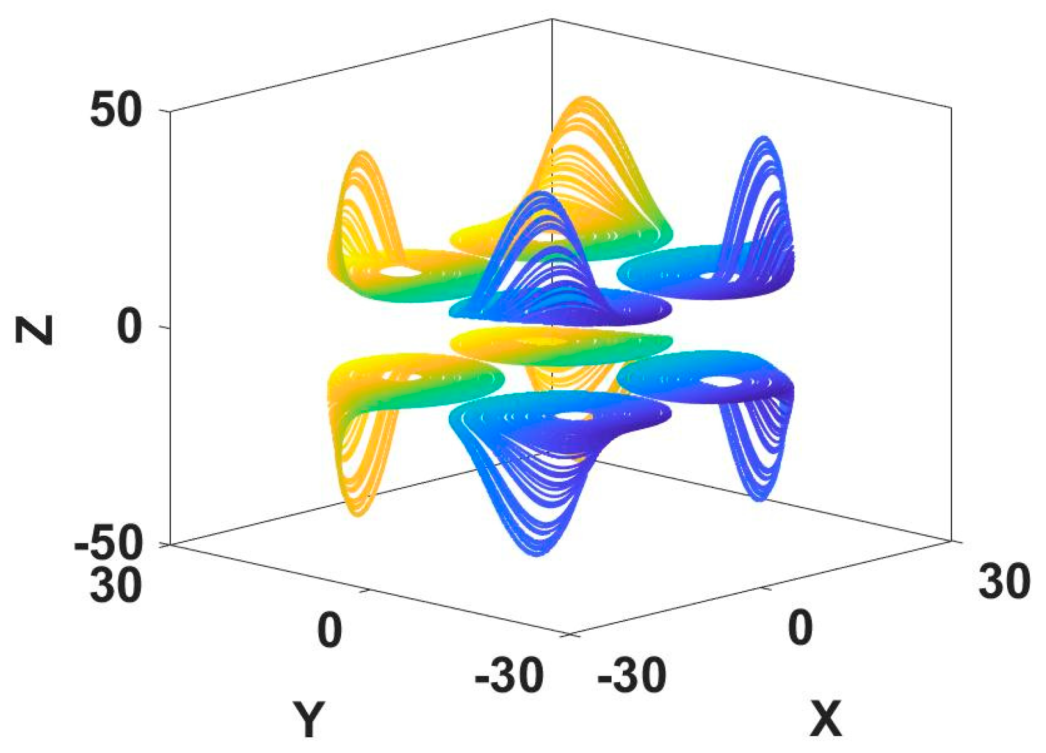
Figure 14.
Polarity balance in a dynamical system.
Figure 15.
Coexisting conditional reflection symmetric attractors of system (10) with IC1 = (3, −1.5, −2) (red), IC2 = (3, −1.5, 1) (green): (a) x−z, (b) y−z.
Figure 15.
Coexisting conditional reflection symmetric attractors of system (10) with IC1 = (3, −1.5, −2) (red), IC2 = (3, −1.5, 1) (green): (a) x−z, (b) y−z.
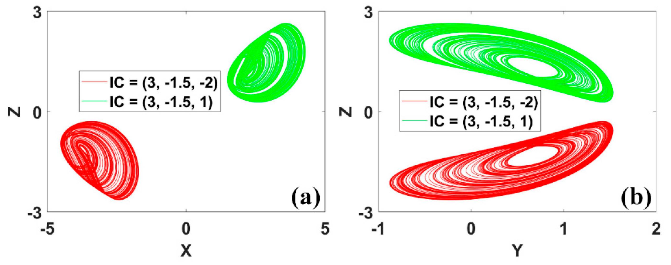
Figure 16.
Coexisting conditional rotational symmetric attractors of system (11) with IC1 = (3, 1, 0.5) (red), IC2 = (−3, 1, 0.5) (green): (a) x−y, (b) x−z.
Figure 16.
Coexisting conditional rotational symmetric attractors of system (11) with IC1 = (3, 1, 0.5) (red), IC2 = (−3, 1, 0.5) (green): (a) x−y, (b) x−z.
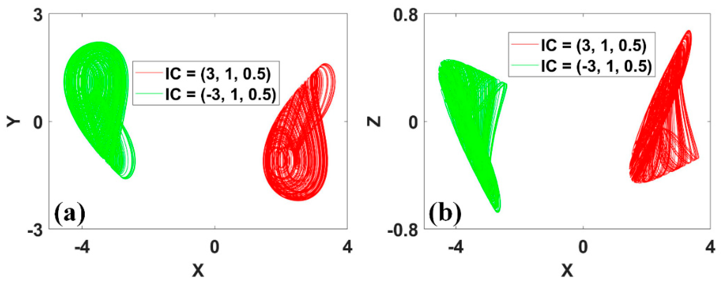
Figure 17.
Coexisting attractors in system (12) by 2D offset boosting, when a = 0.22 and IC1 = (2, 6, −1) (red), IC2 = (−1, 1, −1) (green): (a) x−z, (b) y−z.
Figure 17.
Coexisting attractors in system (12) by 2D offset boosting, when a = 0.22 and IC1 = (2, 6, −1) (red), IC2 = (−1, 1, −1) (green): (a) x−z, (b) y−z.
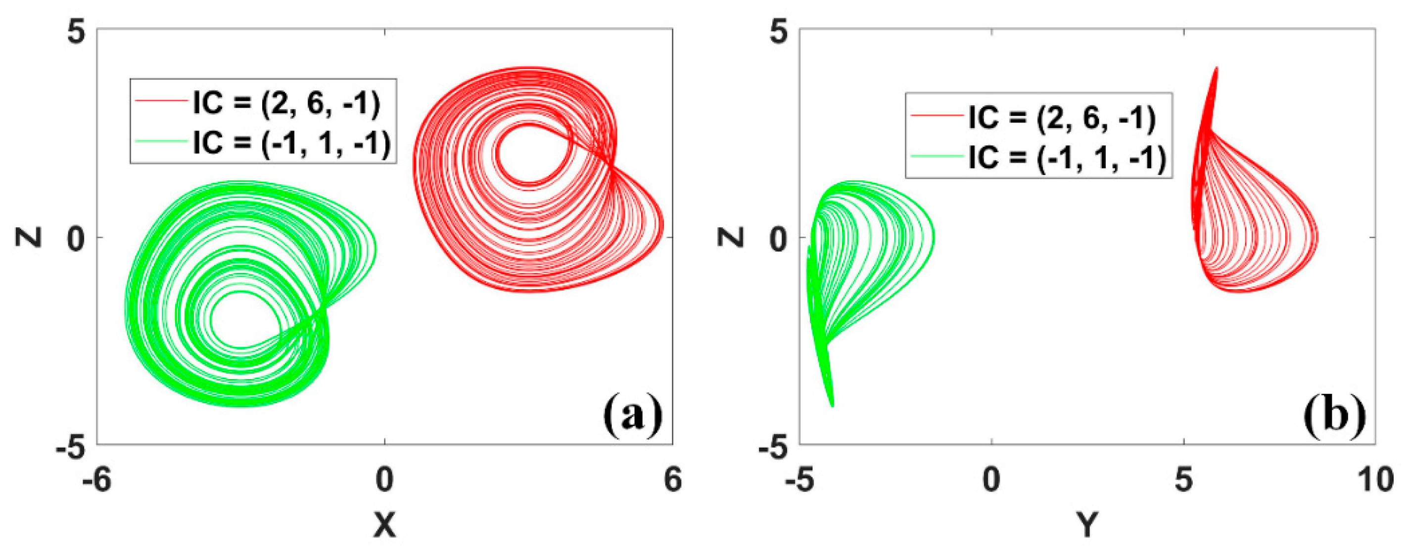
Figure 18.
Coexisting conditional rotational symmetric attractors of system (13) with a = 0.35, IC1 = (0, 0.4, 6) (red), IC2 = (0, 0.4, −5) (green): (a) x−z, (b) y−z.
Figure 18.
Coexisting conditional rotational symmetric attractors of system (13) with a = 0.35, IC1 = (0, 0.4, 6) (red), IC2 = (0, 0.4, −5) (green): (a) x−z, (b) y−z.
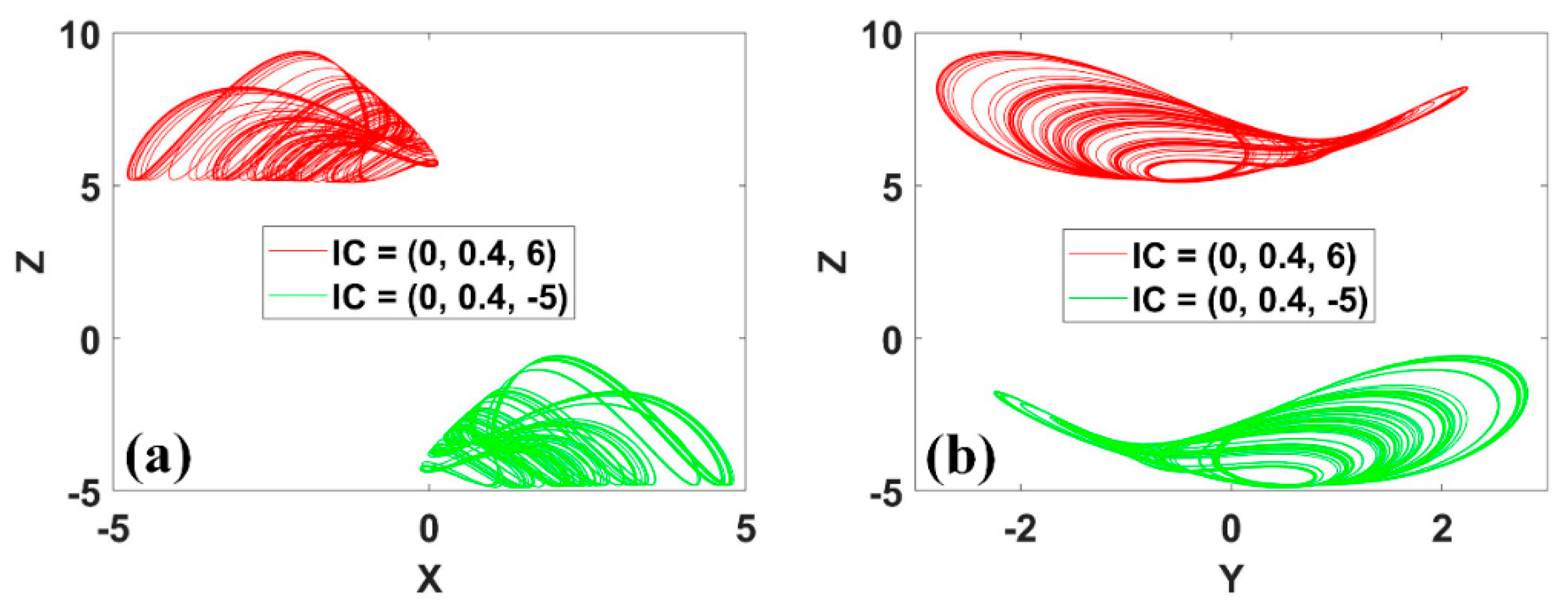
Figure 19.
Coexisting attractors in conditional symmetric system (14) with a = 0.4, b = 1, IC1 = (0, 14, 17) (red), IC2 = (0, −6, −7) (green): (a) x−y, (b) x−z.
Figure 19.
Coexisting attractors in conditional symmetric system (14) with a = 0.4, b = 1, IC1 = (0, 14, 17) (red), IC2 = (0, −6, −7) (green): (a) x−y, (b) x−z.
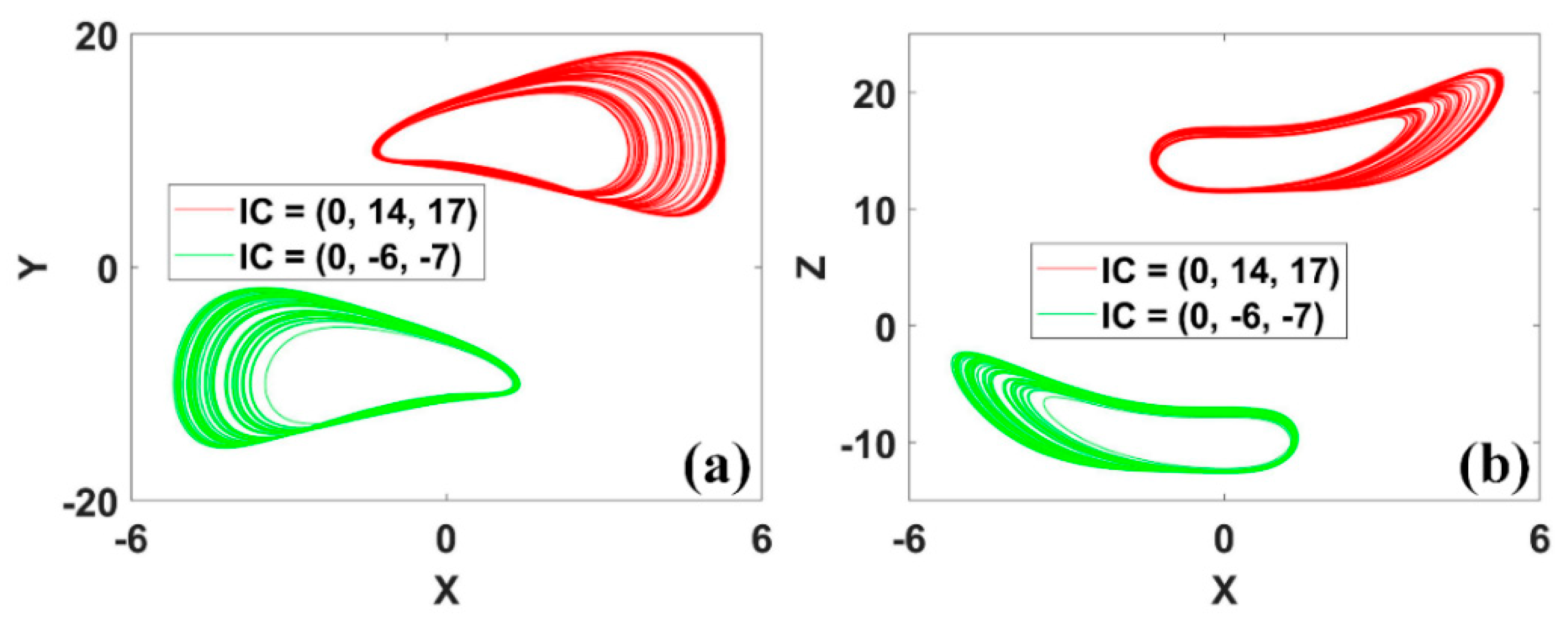
Figure 20.
Coexisting attractors in symmetric system (15) with IC1 = (1, 5, 5.5) (red), IC2 = (1, −5, −4.5) (green): (a) x−z, (b) y−z.
Figure 20.
Coexisting attractors in symmetric system (15) with IC1 = (1, 5, 5.5) (red), IC2 = (1, −5, −4.5) (green): (a) x−z, (b) y−z.
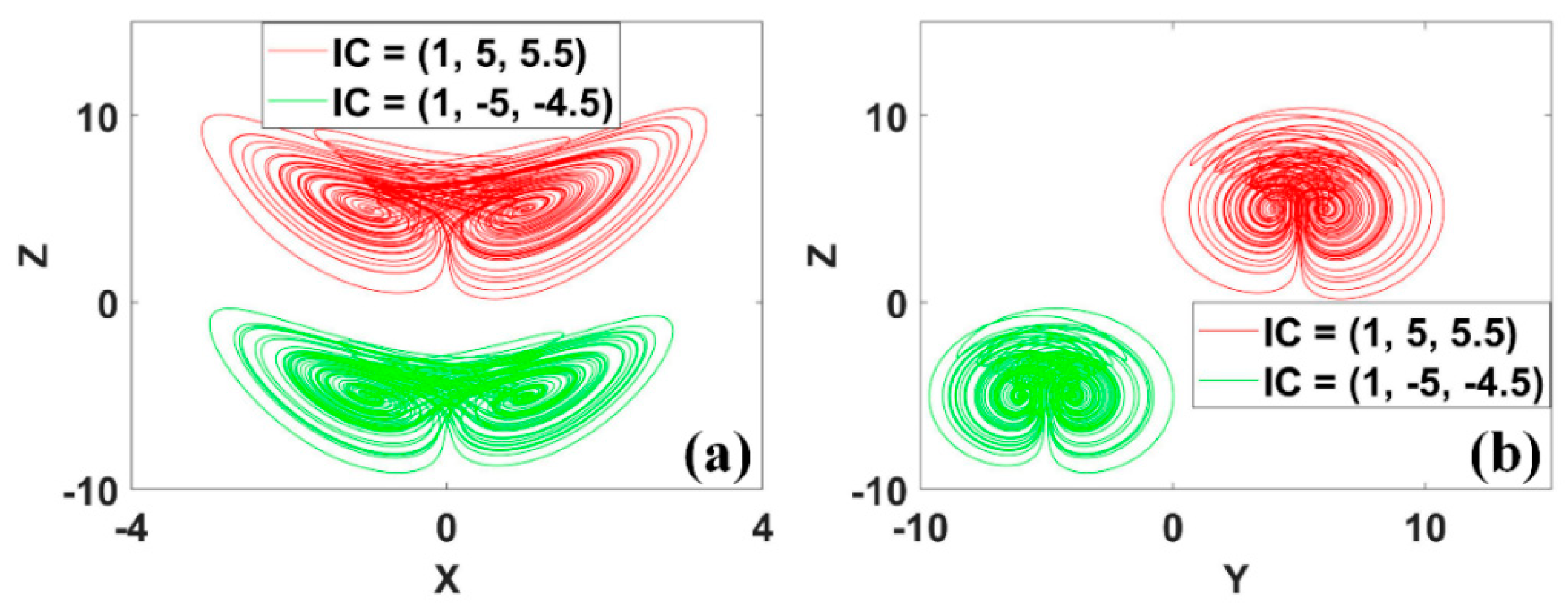
Figure 21.
Coexisting repellors with conditional symmetry in system (16): (a) y−x, (b) z−x. (IC = (0, 0.96, 0) is red, IC = (6, 2, 2) is yellow, IC = (0, −0.96, 0) is green, IC = (−6, −2, −2) is blue.)
Figure 21.
Coexisting repellors with conditional symmetry in system (16): (a) y−x, (b) z−x. (IC = (0, 0.96, 0) is red, IC = (6, 2, 2) is yellow, IC = (0, −0.96, 0) is green, IC = (−6, −2, −2) is blue.)
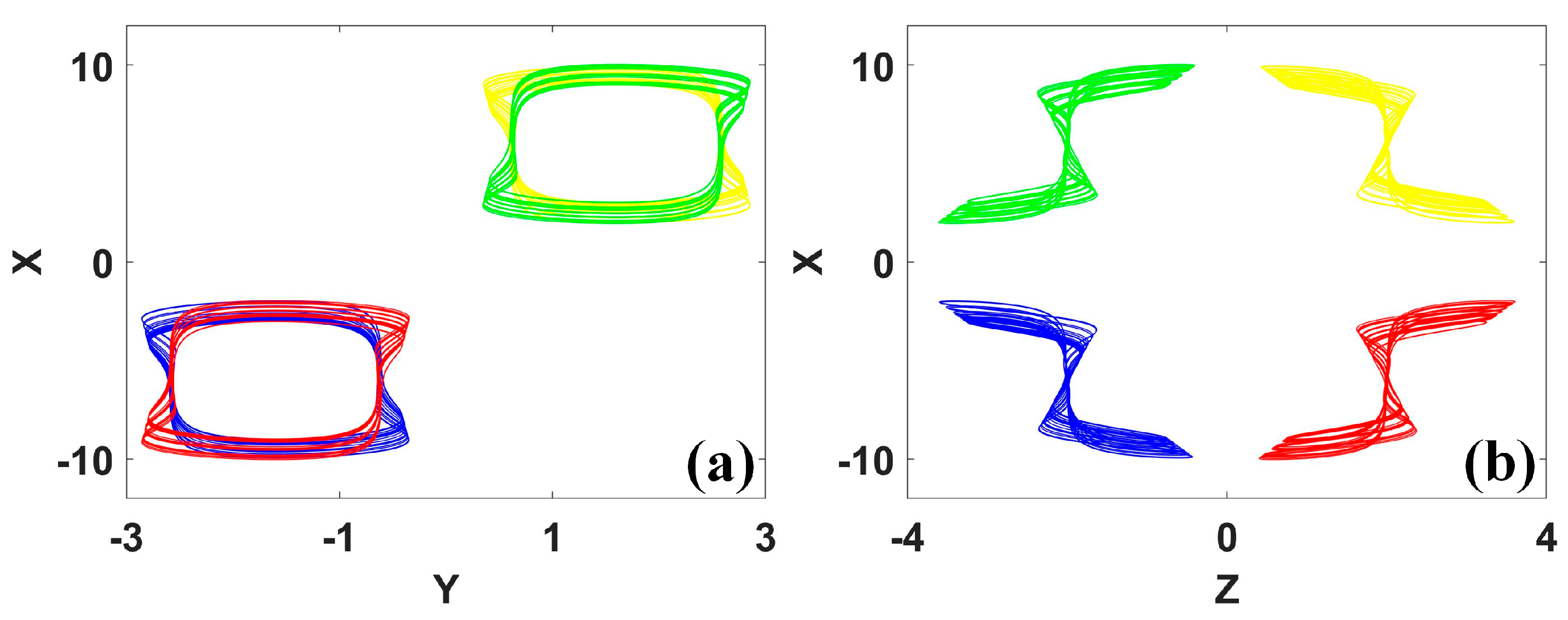
Figure 22.
Coexisting attractors in system (17): (a) x−y, (b) x−z. (IC = (1, 0, 0) is green, IC = (1+1.25π, 0, 0) is pink, IC = (1+2.5π, 0, 0) is red, IC = (1−1.25π, 0, 0) is cyan, IC = (1−2.5π, 0, 0) is blue.)
Figure 22.
Coexisting attractors in system (17): (a) x−y, (b) x−z. (IC = (1, 0, 0) is green, IC = (1+1.25π, 0, 0) is pink, IC = (1+2.5π, 0, 0) is red, IC = (1−1.25π, 0, 0) is cyan, IC = (1−2.5π, 0, 0) is blue.)
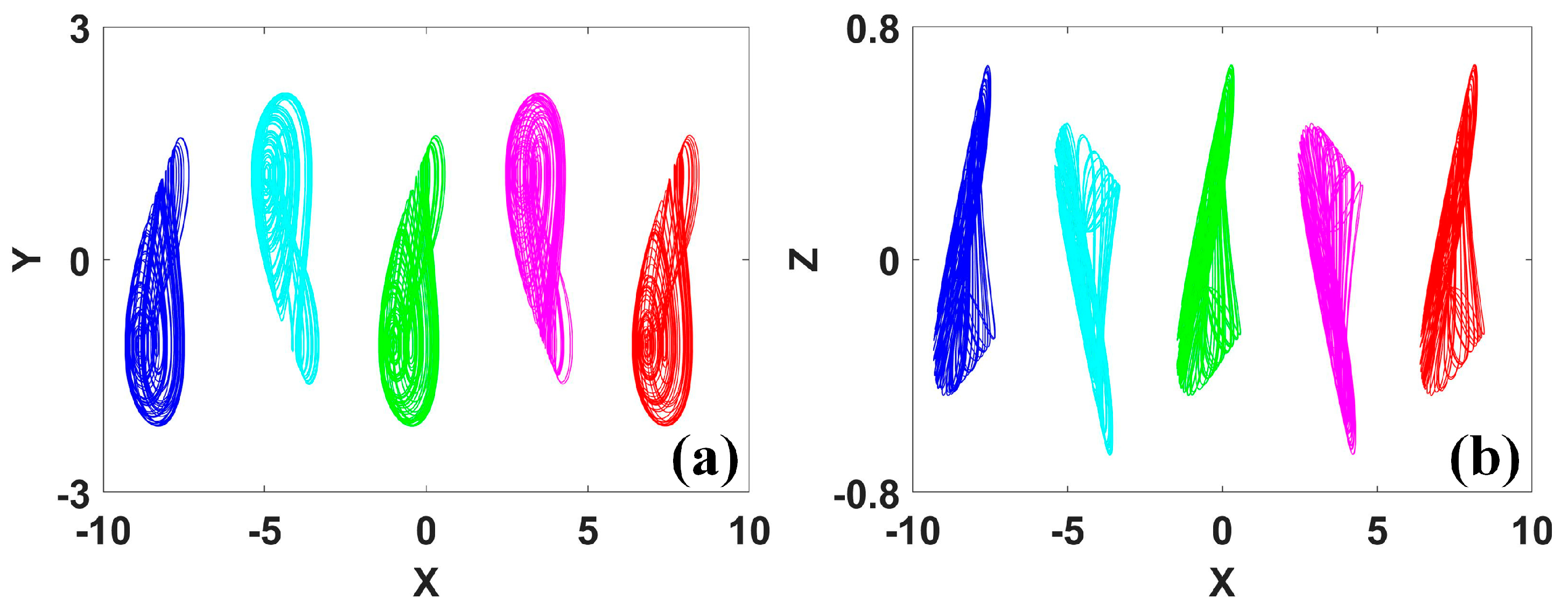
Figure 23.
‘A square earth with a round sky above’ and two types of circuit constraints.
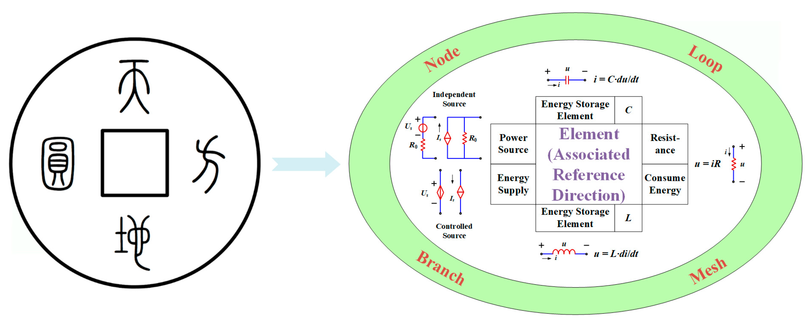
Figure 24.
A simple series chaotic circuit with a memristor, an inductor and a capacitor.
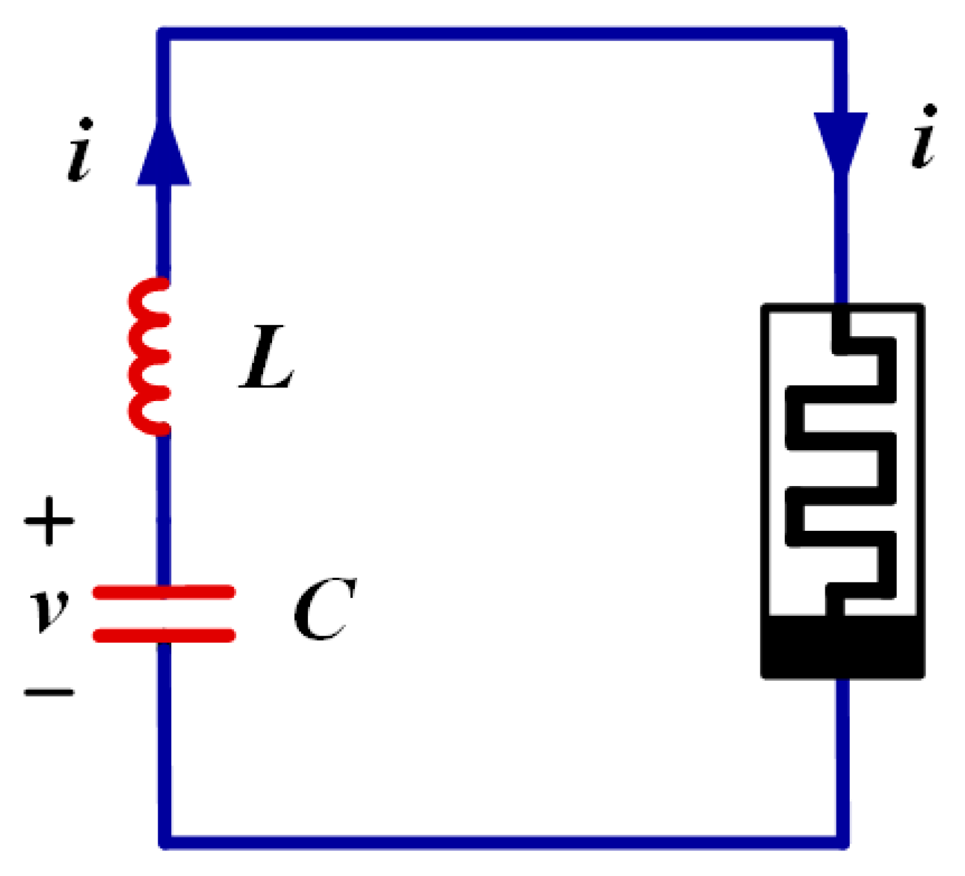
Figure 25.
Symmetric attractor in system (18) with α = 1, ω = 1 and IC = (4.1, 0.7, 5): (a) x−y, (b) y−z.
Figure 25.
Symmetric attractor in system (18) with α = 1, ω = 1 and IC = (4.1, 0.7, 5): (a) x−y, (b) y−z.
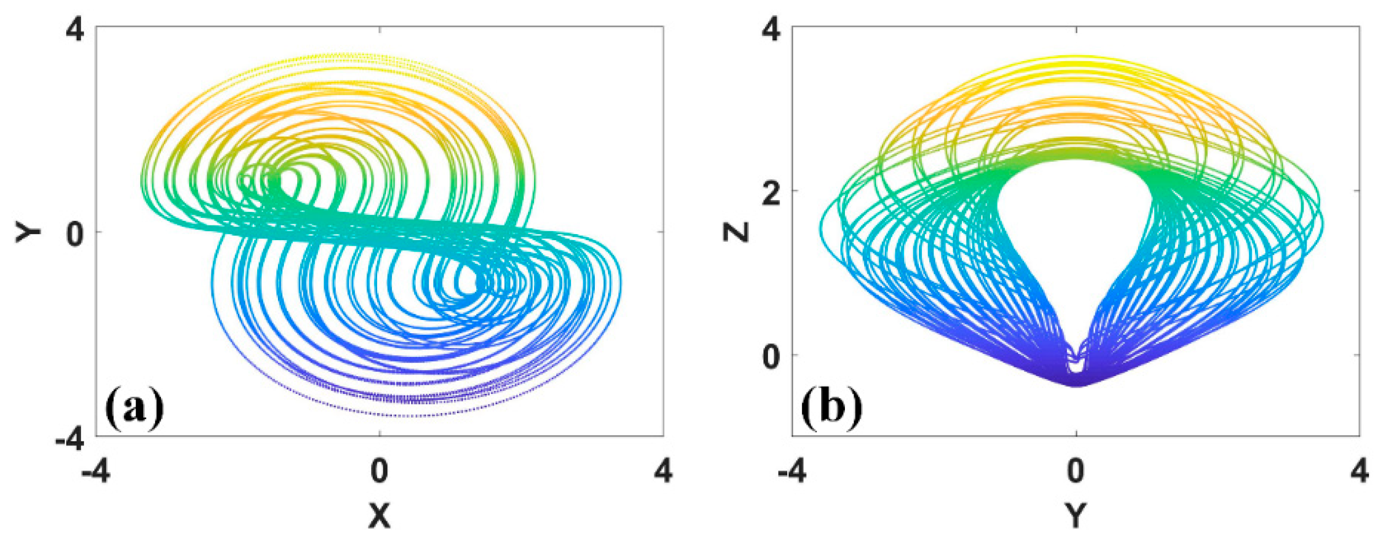
Figure 26.
Conditional symmetric chaotic attractors of system (19) with a = 0.6, b = 1, c = 2, (a) z-y, (b) z-x. (IC = (2, 0, −1) is up, IC = (−2, 0, 1) is down.)
Figure 26.
Conditional symmetric chaotic attractors of system (19) with a = 0.6, b = 1, c = 2, (a) z-y, (b) z-x. (IC = (2, 0, −1) is up, IC = (−2, 0, 1) is down.)
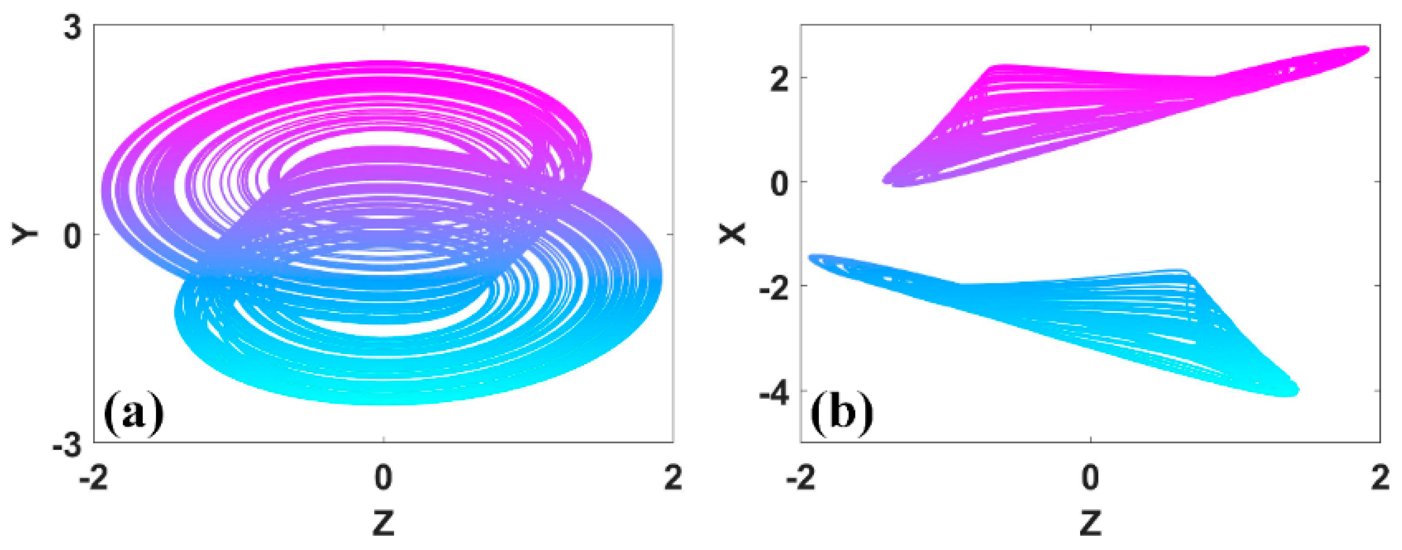
Figure 27.
Meminductive parallel chaotic circuit for realizing system (19).
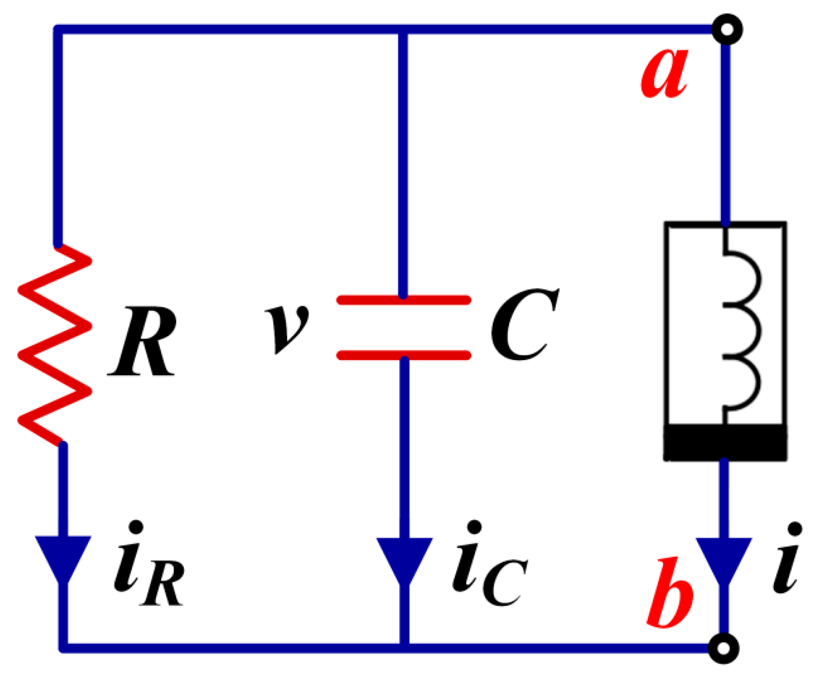
Figure 28.
Conditional symmetric chaotic attractors of system (19) with a = 0.6, b = 1, c = 2 observed in oscilloscope, (a) z-y, (b) z-x. (IC = (2, 0, −1) is green, IC = (−2, 0, 1) is brown.)
Figure 28.
Conditional symmetric chaotic attractors of system (19) with a = 0.6, b = 1, c = 2 observed in oscilloscope, (a) z-y, (b) z-x. (IC = (2, 0, −1) is green, IC = (−2, 0, 1) is brown.)
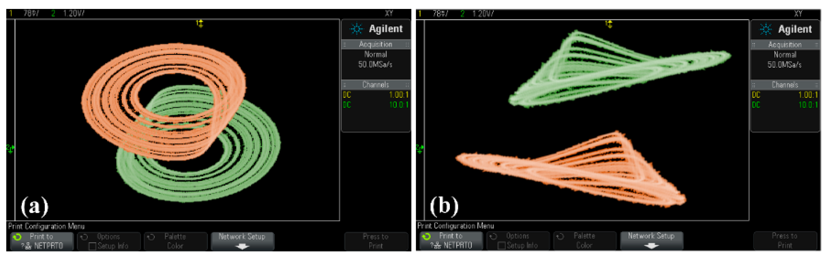
Figure 29.
Chaotic attractors in system (20) with a = 0.6, b = 1, c = 1, d = 4.11 and IC = (1, 1, −1), here two coexisting attractors close each other and bond to be a pseudo-double-scroll attractor: (a) x−y, (b) x−z.
Figure 29.
Chaotic attractors in system (20) with a = 0.6, b = 1, c = 1, d = 4.11 and IC = (1, 1, −1), here two coexisting attractors close each other and bond to be a pseudo-double-scroll attractor: (a) x−y, (b) x−z.
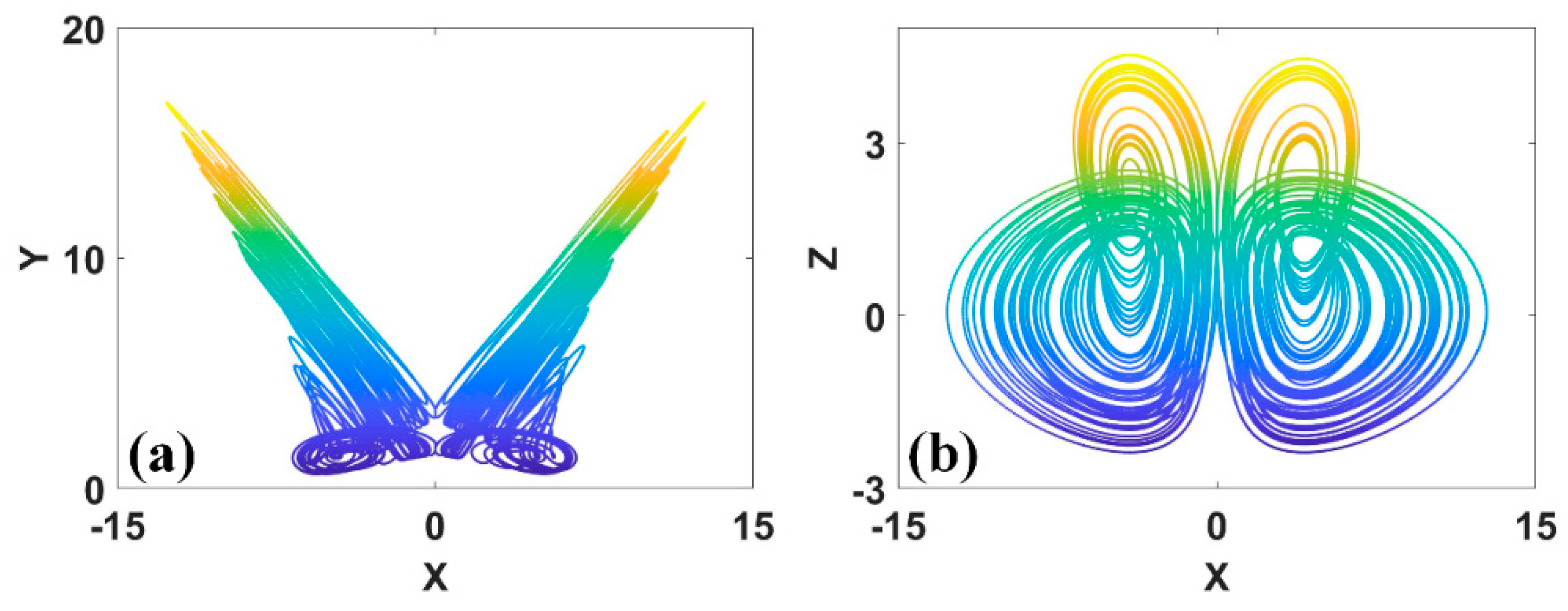
Figure 30.
Coexisting attractors of system (20) with a = 0.6, b = 1, c = 1, d = 8: (a) x−y, (b) x−z. (IC = (−1, 1, −1) is left, IC = (1, 1, −1) is right.)
Figure 30.
Coexisting attractors of system (20) with a = 0.6, b = 1, c = 1, d = 8: (a) x−y, (b) x−z. (IC = (−1, 1, −1) is left, IC = (1, 1, −1) is right.)
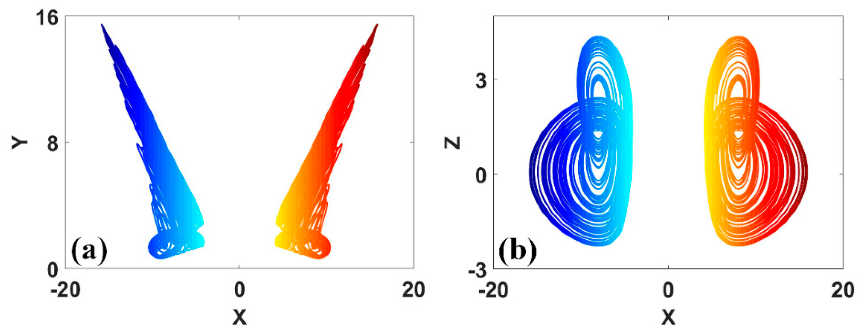
Figure 31.
Simple circuit operation unit: (a) multiplier current constraint under external resistance, (b) the resistor-capacitor coupling realizes current control.
Figure 31.
Simple circuit operation unit: (a) multiplier current constraint under external resistance, (b) the resistor-capacitor coupling realizes current control.

Figure 32.
Schematic circuit of the system (21).
Disclaimer/Publisher’s Note: The statements, opinions and data contained in all publications are solely those of the individual author(s) and contributor(s) and not of MDPI and/or the editor(s). MDPI and/or the editor(s) disclaim responsibility for any injury to people or property resulting from any ideas, methods, instructions or products referred to in the content. |
© 2023 by the authors. Licensee MDPI, Basel, Switzerland. This article is an open access article distributed under the terms and conditions of the Creative Commons Attribution (CC BY) license (http://creativecommons.org/licenses/by/4.0/).
Copyright: This open access article is published under a Creative Commons CC BY 4.0 license, which permit the free download, distribution, and reuse, provided that the author and preprint are cited in any reuse.


