

Submitted:
03 July 2023
Posted:
04 July 2023
You are already at the latest version
Preprints on COVID-19 and SARS-CoV-2
Abstract
Our aim is to provide an insight of the procedures and the dynamics that lead the spread of contagious diseases through populations. Our simulation tool can increase our understanding on the spatial parameters which affect the diffusion of a virus. SIR models are based on the hypothesis that populations are “well mixed”. Our model constitutes an attempt to focus on the effects of the specific distribution of the initially infected individuals through the population and provide insights, considering the stochasticity of the transmission process. For this purpose, we represent the population using a square lattice of nodes. Each node represents an individual that may or may not carry the virus. Nodes that carry the virus can only transfer it to susceptible neighboring nodes. This important revision of the common SIR model provides a very realistic property: the same number of initially infected individuals can lead to multiple paths, depending on their initial distribution in the lattice. This property creates better predictions and probable scenarios to construct a probability function and appropriate confidence intervals. Finally, this structure permits realistic visualizations of the results to understand the procedure of contagion and spread of a disease and the effects of any measures applied.
Keywords:
COVID-19
; SARS-CoV-2
; epidemiology
; lattice simulation
; infection diffusion
; epidemics
; control measures
1. Introduction
This research aims to provide a supplementary tool, improving our ability to understand, trace and present the epidemic and pandemic spread of viruses on populations, considering specific spatial information. Our main purpose is to provide an appropriate model to understand the diffusion mechanisms and the effects of different population characteristics and restrictive measures as accurately as possible.
As a reference, we used parameters that are estimated as applicable on COVID-19 in Greece. It is an appropriate example, since it constitutes a Corona-Virus-Disease (COVID), observed during the last days of 2019. An individual can get infected by close contact or being in indoor settings or even by touching contaminated surfaces or objects. Carriers can be symptomatic or asymptomatic. Both categories can become contagious. One year later, the first vaccine was available, while up to now, nine of them are approved [1].
The most common model to approach the spread of a virus disease is using SIR models [2]. A homogenous population of size N is divided into three groups: Susceptible (S), Infected (I) and Removed (R). Susceptible individuals can get infected by contagious Infected individuals, while Infected individuals can get Removed, either recovered (and immune) or dead. Obviously, at any given time t:
Continuous time epidemic models, as SIR, are usually applied to describe the dynamics of transmission of infectious diseases, because of their tractability [3,4,5]. Additional conditions are allowed in more recent models. In the case of another Corona-Virus syndrome, which outbroke in South Korea, the model additionally included: Exposed to the virus (E), Asymptomatic carriers (A) and Hospitalized heavy diseased individuals (H) [6].
Although, difference equations are also appropriate since they could be directly applicable to time-series data [5], we choose to work using a simulation, which might be more accurate and adapted to time-series data available if a discretized model is used [7].
The model works as follows: Susceptible individuals might become Exposed, if they contact Infected or Asymptomatic individuals. After an incubation period, Exposed individuals become infectious-contagious. Some of them are symptomatic (Infected), while others are Asymptomatic. Some of the symptomatic individuals get Hospitalized, and all Asymptomatic, Infected and Hospitalized move to Removed (recover or die).
Recent research on COVID-19, additionally separated recovered from symptomatic (R), who are observable and recovered from asymptomatic (AR), who cannot be identified easily. They also added a spatial parameter: density of population [8]. This consideration of heterogeneous populations and its effect on the spread of the virus was an inspiration to our research.
Another interesting way to deal with heterogeneity is by separating the population into categories and using contact matrices [9]. One of the potentials of our research is to allow us to divide the population into geographical areas (such as islands or geomorphologically separated regions) and use contact matrices to examine the effects of landscape and restrictions on the transmission of the virus.
On the other hand, there are researchers that use a simulation procedure considering that the density of infected by COVID-19 individuals in a population could be fitted well by a Self-Organizing Diffusion Model (SODM), designed to describe the diffusion of a charge through a lattice. Considering a square lattice of nodes that can be active or inactive (representing carriers or non-carriers), they assign a “charge” instead of the virus on some nodes that become active (carriers). Charge can be transferred to inactive nodes neighboring to an active node [10].
2. Materials and Methods
2.1. Context
We based our model on the initial concept of [10]. Thus, we present an example of its structure using a simple 3x3 square lattice of nodes in Figure 1. It has one active node (A) in the center and 8 inactive nodes (N). The active node could transfer “charge” through any of the red arrows, activating non-active nodes. They also claim [10] that measures of “isolation” reduce the number of the red arrows that transfer “charge”.
Applying this charge diffusion model on epidemics, we represent individuals of the population as nodes. Active nodes could be considered as Infected (I) and inactive nodes as Susceptible (S). We reduce the importance of “charge”, using it only to flag the individual as Infected (represented by 1) and Susceptible (represented by 0). This constitutes a fundamental change of the model, since it becomes able to reproduce the states of Susceptible and Infected individuals and the properties of contagion and immunity in a way that corresponds to the respective terms used in SIR models.
Additionally, we allowed more states than “active”-“infected” and “inactive”-“susceptible”, based on the states that are used in extended SIR models (SEAIR) - we will discuss those states in Section 2.2. On a square lattice of LxL nodes, we “seed” a few infected individuals in random nodes. In every step (sweep), infected nodes might infect some of their susceptible neighboring nodes. Infected nodes (symptomatic or asymptomatic) get temporary immunity after a specific time.
This approach has two interesting and important advantages, compared to common SIR models:
- it considers the initial distribution of the infections, through the lattice-population.
- we can visualize this spread through time and space, making the whole concept easier to understand.
The most important fact is that this model considers three kinds of realistic stochasticity:
- In most of the cases, accurate initial distribution of the infected individuals in the lattice cannot be observed through the existing data, so any considerations are based on random distribution (uniform). To make clear the importance of this property, we return to the simple 3x3 square lattice, dividing population to Infected (I-nodes) and Susceptible (S-nodes) as presented in Figure 2. In the following example, both lattices (Figure 2a and Figure 2b) represent a population of nine nodes-individuals. Two of them are Infected (I0 = 2) and seven are Susceptible (S0 = 7). Let us note that their distribution is not the same. Both diagrams are equally probable to appear but may lead to different paths of the virus spread, because of their initial distribution. SIR models cannot conceive such information. It is obvious that the initial distribution of infected individuals through the lattice determines the number of possible contagions. This way, it affects the reproduction number of the virus. For example, we can verify that the central node of Figure 2a can transmit the virus to up to four neighboring nodes, while the bottom right node of Figure 2b can only affect one node maximum. Additionally, if contagions represented by arrows happen with a probability less than 1, then susceptible individuals have different probabilities of getting infected. For example, the susceptible nodes of the second column of Figure 2a would have different probabilities of getting infected in such a case. The first-row node is exposed to two separate contagious individuals, while the third-row node is exposed to one contagious individual.
- A second realistic stochasticity is related to susceptible individuals who can contact infected ones after every sweep (period). Some contacts may meet while others won’t (considering restrictions on mobility, self-protection measures, isolation etc.). We only allow, for a percentage of those possible contacts, to transform susceptible individuals to exposed, while the rest get away with no contagion. We use a random process, so that contact is enabled only for two neighboring nodes of each infectious node. In the example presented in Figure 3, only up and right neighboring nodes can get infected. Although, in the first (Figure 3a) case both interactions lead to infections, while in the second (Figure 3b) case, one of them is already infected so only the other interaction leads to a new infection.
- The third realistic stochasticity presented in our model, allows some exposed individuals to evolve to be asymptomatic, while the rest evolve to be infected (symptomatic). Both situations lead to immunity, after some days (sweeps).
Finally, having tested a lot of scenarios and models, we ended up with a better structured model, which works as follows. Let us divide contagious individuals to: Infected (I) and Asymptomatic (A). Susceptible (S) individuals might become Exposed (E) when they contact Infected or Asymptomatic individuals. After an incubation period, Exposed individuals become infectious-contagious. Some of them are symptomatic (Infected), while others are Asymptomatic. Infected and Asymptomatic individuals move to Removed (R) and Asymptomatic Removed (AR) respectively, obtaining immunity. In this version of the model, we excluded deaths for simplicity.
All the above stochastic elements allow different paths to rise by the same initial conditions. This is one of the most important facts that makes this model a useful tool and offers an additive value to the existing literature.
2.2. Experimentation
We started exploring the potential of our model, using MATLAB [11]. We initially based our research on the model of [10], so we used a lattice of nodes, representing a population of individuals, respectively. We transformed it in a way that it could:
- become able to estimate the number of infected and susceptible individuals and represent those states clearly, by replacing charge with flag values. We used 1 for Infected and 0 for Susceptible. Diffusion of charge is replaced by contagion of virus to neighboring nodes-individuals,
- apply to an extended SIR model (we experimented using SEAIR). Except for values 1 and 0, for Infected (I) and Susceptible (S) respectively, we used 0.5 for Exposed (E), 0.75 for Asymptomatic (A) and -0.25 and -0.5 for Asymptomatic who Recovered (AR) and Infected who Recovered (R) respectively,
- visualize results. Our model’s results can be depicted in short videos, presenting the lattice from day one (initial condition) to the final day. An observer can identify the exact coordinates of each infection and recovery and understand patterns of contagion and immunity building in the population.
Our initial approach was focused on small lattices. An interesting size that is small but representative of the properties of our model is the 6x6 lattice. We present here two different cases, both starting with 3 infected individuals, in different places on the lattice. We observe its evolution for 120 days. Even if the lattice is small, the difference of the paths is obvious. Then we apply our model on a 100x100 lattice starting with 117 infected individuals for 200 days and we extensively analyze the results and insights that can be extracted.
Even though we’ve just been experimenting, we used parameters based (approximately) on the results of COVID-19 in Greece during the first months of its outbreak, in 2020 [8]. It became clear that those parameters should be corrected for our model, since we have to consider that new infections of each period are neighboring to old ones, leading to an important reduction of the effective reproductive number implied. At this point, we ignored hospitalization and death, considering that disease ended by recovery and immunization. The parameters we used are presented in Table 1.
At last, we tried to approximate the Greek population (10,768,477 individuals), by a square lattice of 3282x3282 dimensions. In this case we used the initial condition of 117 Infected individuals (March 12th, 2020, according to [8]) and tracked its evolution for 1000 days (up to December 7th, 2022). The data are – reasonably - not fitting reality, since we have not applied any measures like quarantine, mobility restrictions and vaccination.
3. Results
We used our model to estimate and visualize three different populations, using a 6x6 lattice, a 100x100 lattice and a 3282x3282 lattice. We focused on the second one to extract and present the insights that can be obtained by applying this model. We suggest that our model is especially appropriate to identify a confidence interval for the evolution of the spread of a virus in a population. It can also reveal extraordinary but possible scenarios, based on any given initial conditions and parameters.
3.1. 6x6 Lattice
We use this relatively small and simple infrastructure to briefly explain the mechanisms and properties used in the model we created. In this presentation we have created two videos that use the same parameters and initial conditions, although the stochastic nature of our simulations allows for differences in the contagion and immunization process.
We observe that both Figure 4 (Video S1) and Figure 5 (Video S2) start having , and . Parameters are the same for both videos. In Figure 4 (Video S1), Infected individuals increase fast. It reaches up to 9 individuals simultaneously. After day 20, the virus disappeared. In Figure 5 (Video S2) we observe a maximum number of infected individuals equal to 4. It takes more than 35 days to reach zero cases. These important observed differences are strong arguments that support the use of our model to analyze the evolution of epidemics in populations.
A different scenario, using the same parameters and initial conditions is presented in Figure 5 (Video S2).
3.2. 100x100 Lattice
In larger lattices of more nodes, such as 100x100, differences become more clear and wider. The following two videos, Figure 6 (Video S3) and Figure 7 (Video S4), depict the paths of two populations with an initial “seeding” of 117 Infected cases in different initial positions. We observed those populations for 200 days. Again, there is an important difference in the days passed before the virus stops spreading and a difference in the height of the peaks of infected individuals.
In Figure 7 (Video S4), we depict the differences that can appear when the initially infected individuals are in different places in the lattice.
In Figure 6 (Video S3), Infected individuals increase fast. It reaches a maximum of more than 400 individuals simultaneously, in less than 20 days. Before day 100, the virus disappeared. In Figure 7 (Video S4) we observed a maximum number of infected individuals below 400 individuals. 200 days after the initial time, there are still a few infected individuals. Again, we claim that those different paths are not possible to be observed or even identified without a simulation model that accounts for realistic stochastic processes that affect the evolution of the system.
After running 100 different scenarios of the initial distribution of the 117 Infected individuals, we can observe that the paths clearly follow a specific pattern, but differences are not insignificant to be ignored. Having the same number of initially infected individuals, placed on the same lattice, we observed that the maximum number of simultaneously infected varies between 340 and 450 cases, standing for more than 25% fluctuation, only after running 100 simulations. The time series of estimated infected individuals for 100 scenarios are presented in Figure 8.
Figure 8 makes clear that stochasticity plays a significant role in this procedure, and it should be considered while planning best response policies. An important difference that appeared is that the same initial conditions led most trajectories to one wave of the epidemic, while others included a second, less intense wave. Especially in Video S4 we can observe an endemic behavior of the virus spread.
To better present the utilities of our model, we found it useful to depict in Figure 9 the histogram of maximum infected individuals (at the same time) in all 100 scenarios.
This information allows policy makers to identify the probability of scenarios that get ahead specific tolerance thresholds. For example, we can claim that the estimated probability of having a peak above 438 infected individuals is less than 4%.
3.3. 3282x3282 Lattice
Moving to a larger and more representative lattice of a country’s population, we used a 3282x3282 lattice. The number of its nodes is almost equal to Greek population. Using 117 Infected people (March 12th, 2020) as initial condition in various places, we observed different results. We observed those populations for 1000 days. In Figure 10 (Video S5), we depict a representative case.
The capacity of this population allows for an extremely different path, comparing to the case of the 100x100 lattice, although I0 = 117 was still the initial condition. Observing the image of the lattice on the first day in this case, the 117 Infected individuals are almost impossible to be identified. Soon, contagion creates clusters of Infected and Recovered individuals, unveiling the location of the initial cases. After 1000 days, without intervention (restrictions, measures, vaccination) the number of active Infected individuals is increasing rapidly, reaching 120,000.
4. Discussion
Our multiple observations suggest that this way of modeling and visualizing the spread of COVID-19 can become helpful in understanding the range of different paths, rising by the same initial conditions. We do not claim that this approach must replace traditional SIR models, but we suggest that it contributes to a better understanding of stochasticity, while it allows researchers to define proper probabilities on different paths, emerging from the same initial conditions, using a sufficiently large number of simulations (according to Monte Carlo method).
Since the data on the accurate location and interconnections of Infected individuals are rarely available, SIR based models remain useful, but multiple simulations using our model allow the researchers to obtain a wider and more inclusive perspective of the situation.
We also suggest that the visualization of the forecasted paths can allow non familiar with virus spread audiences to better understand the situation and the reasons leading to any measures applied.
Our future steps include the application of this model on COVID-19 spread and vaccination in Greece, with an emphasis on the small islands of Greece, where location and (almost natural) isolation of small populations makes such simulations very useful to understand the dynamics of the epidemics.
5. Conclusions
We observed that the size of the population -lattice- and the specific location of the initially Infected individuals in the population lattice is critical to the evolution and the spread of the infections. The duration, the intensity of the pandemic and the number of waves seem to extensively depend on those initial conditions, a property that is fundamentally ignored by the SIR and extended SIR models. We suggest a method that allows interested parties to understand and better explain the probabilities of different scenarios and, thus, improve the ways to predict and prevent the expansion of spreading diseases and viruses. Visualization of the results might become a useful tool to explain and communicate the diffusion of the infections through a population to not so familiar audiences, convincing them to act in accordance to any given situation and prevent unhealthy behaviors or overreacting.
Author Contributions
Conceptualization, Loukas Zachilas; Investigation, Christos Benos; Methodology, Christos Benos; Project administration, Loukas Zachilas; Software, Christos Benos; Supervision, Loukas Zachilas; Validation, Christos Benos; Writing – original draft, Christos Benos
Funding
This research was funded by H.F.R.I. (Hellenic Foundation for Research and Innovation) (Proposal ID: 05138) under the Action: “HFRI Science & Society: Interventions to address the economic and social consequences of the COVID-19 pandemic”.
Acknowledgments
The authors would like to thank Prof. St. Stavrinides for providing the code (originally written in FORTRAN) and successfully translated to Matlab by the second author.
Conflicts of Interest
The authors declare no conflict of interest.
References
- World Health Organization, Coronavirus disease (COVID-19). Available online: https://www.who.int/emergencies/diseases/novel-coronavirus-2019 (accessed on 30 June 2023).
- Kermack, W.O.; McKendrick, A.G. A contribution to the mathematical theory of epidemics. In Proceedings of the Royal Society of London, Series A 1927, 115, 700–721. [Google Scholar] [CrossRef]
- Lajmanovich, A.; Yorke, J. A. A deterministic model for gonorrhea in a nonhomogeneous population. Math. Biosci. 1976, 28, 221–236. [Google Scholar] [CrossRef]
- Nallaswamy, R.; Shukla, J.B. Effects of dispersal on the stability of a gonorrhea endemic model. Math. Biosci. 1982, 61(1), 63–72. [Google Scholar] [CrossRef]
- Allen, L.J.; Kirupaharan, N.; Wilson, S.M. SIS epidemic models with multiple pathogen strains. J. of Diff. Eq. and App. 2004, 10(1), 53–75. [Google Scholar] [CrossRef]
- Xia, Z.Q.; Zhang, J.; Xue, Y.K.; Sun, G.Q.; Jin, Z. Modeling the transmission of Middle East respirator syndrome corona virus in the Republic of Korea. PloS one 2015, 10(12), e0144778. [Google Scholar] [CrossRef]
- Ramani, A.; Carstea, A.S.; Willox, R.; Grammaticos, B. Physica A 2004, 333, 278–292. [CrossRef]
- Kevrekidis, P.G.; Cuevas-Maraver, J.; Drossinos, Y.; Rapti, Z.; Kevrekidis, G.A. Reaction-diffusion spatial modeling of COVID-19: Greece and Andalusia as case examples. Physical Rev. E 2021, 104(2), 024412. [Google Scholar] [CrossRef] [PubMed]
- Kadelka, C. Projecting social contact matrices to populations stratified by binary attributes with known homophily, arXiv preprint 2022. arXiv:2207.12328. [CrossRef]
- Contoyiannis, Y.; Stavrinides, S.G.P.; Hanias, M.; Kampitakis, M.; Papadopoulos, P.; Picos, R.; Potirakis, M.S. A Universal Physics-Based Model Describing COVID-19 Dynamics in Europe. Int. J. of Env. Res. and Pub. Health 2020, 17(18), 6525. [Google Scholar] [CrossRef] [PubMed]
- MATLAB. Ver. 9.9.0 (R2020b). Natick, Massachusetts, The MathWorks Inc.
Figure 1.
A 3x3 lattice of 9 nodes. The central node is initially active (A) (infected) and may transmit the virus to the four nodes (N) (non-infected) pointed by the red arrows.
Figure 1.
A 3x3 lattice of 9 nodes. The central node is initially active (A) (infected) and may transmit the virus to the four nodes (N) (non-infected) pointed by the red arrows.

Figure 2.
Two 3x3 lattices of nodes (a) and (b) representing populations. Red arrows represent the possible contagions. In both nodes, there are two initial infected people (I0 = 2), while seven are Susceptible (S0 = 7). In (a) there are four Infected nodes, while in (b) there are three.
Figure 2.
Two 3x3 lattices of nodes (a) and (b) representing populations. Red arrows represent the possible contagions. In both nodes, there are two initial infected people (I0 = 2), while seven are Susceptible (S0 = 7). In (a) there are four Infected nodes, while in (b) there are three.
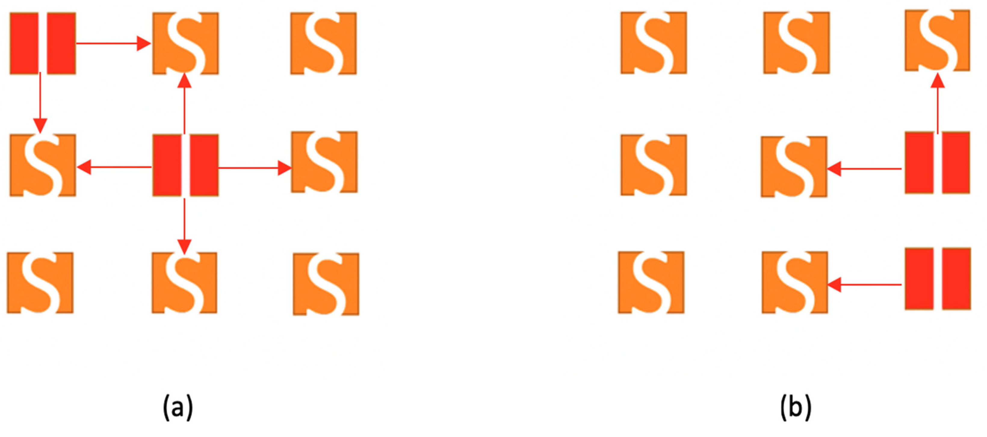
Figure 3.
Two 3x3 lattices of nodes (a) and (b) representing populations. Arrows represent the possible contagions. Green arrows represent contacts that will lead to contagion. Red arrows represent contacts that will not lead to contagion. (a) both interactions lead to infections. (b) one of them is already infected so only the other interaction leads to a new infection.
Figure 3.
Two 3x3 lattices of nodes (a) and (b) representing populations. Arrows represent the possible contagions. Green arrows represent contacts that will lead to contagion. Red arrows represent contacts that will not lead to contagion. (a) both interactions lead to infections. (b) one of them is already infected so only the other interaction leads to a new infection.
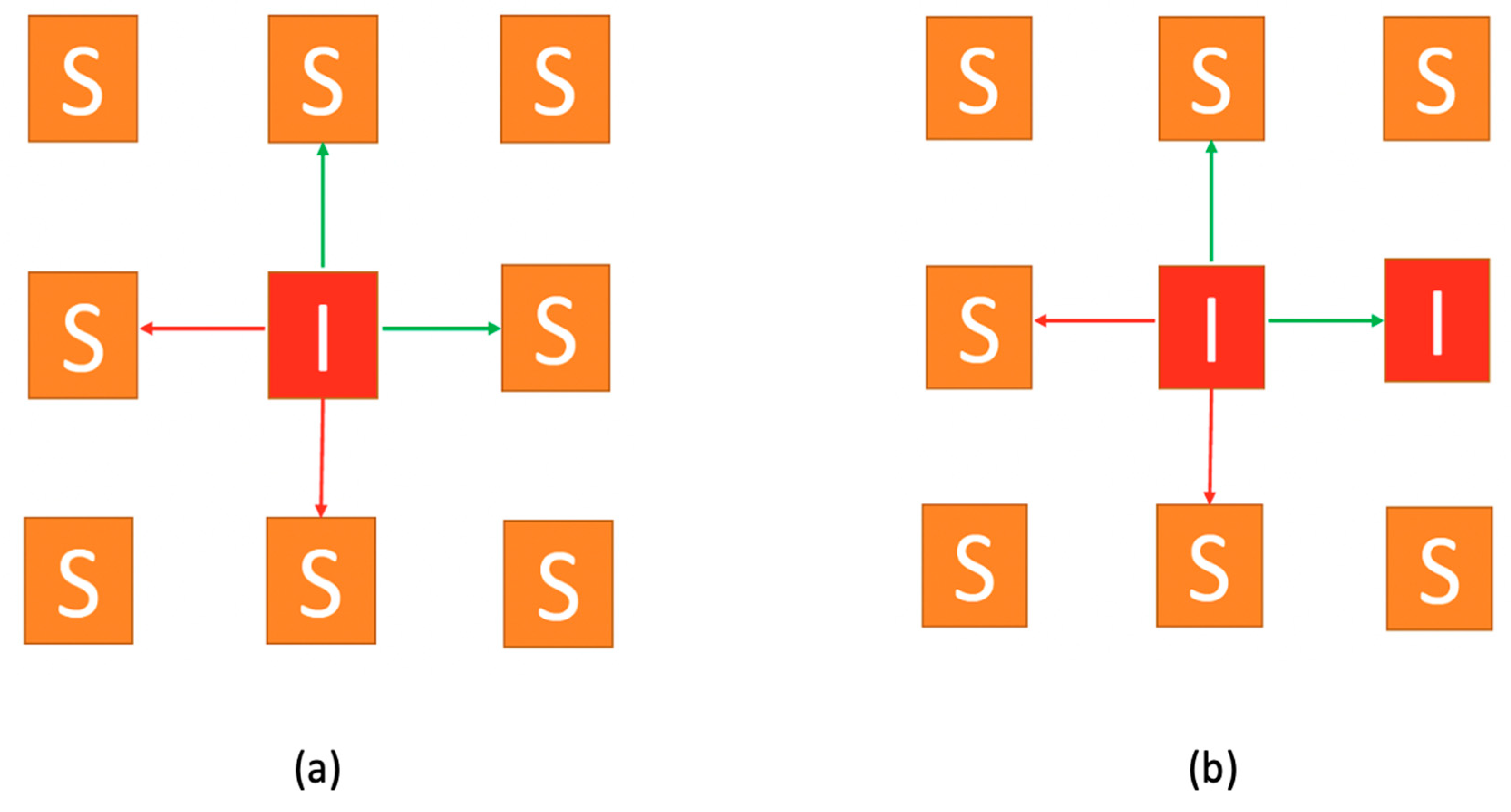
Figure 4.
(Video S1). 6x6 Lattice. and 120 days. On the left, we observe the number of infected individuals through time. On the right, the lattice.
Figure 4.
(Video S1). 6x6 Lattice. and 120 days. On the left, we observe the number of infected individuals through time. On the right, the lattice.
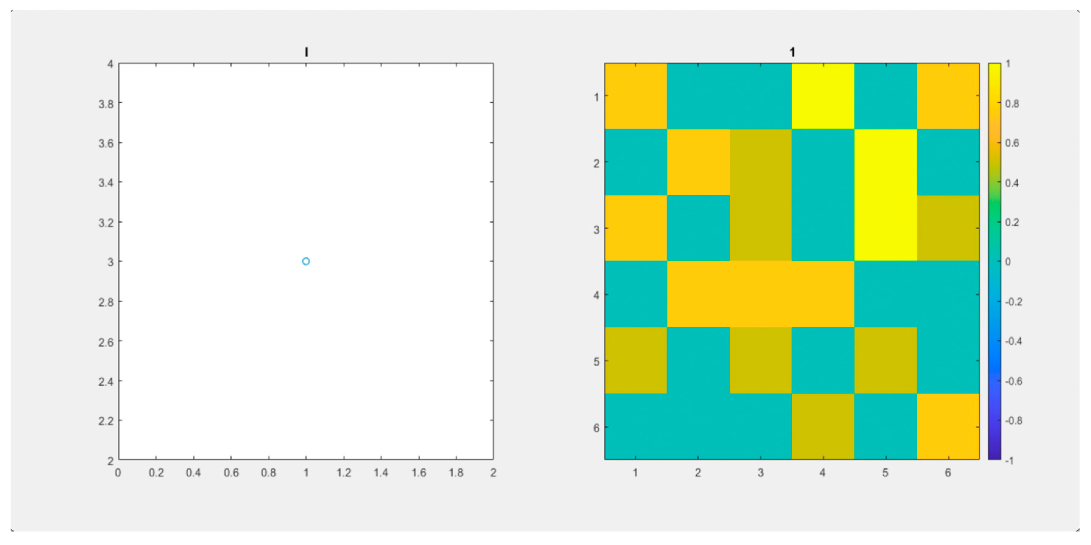
Figure 5.
(Video S2). 6x6 Lattice. and 120 days. Another initial distribution through the lattice. On the left, we observe the number of infected individuals through time. On the right, the lattice.
Figure 5.
(Video S2). 6x6 Lattice. and 120 days. Another initial distribution through the lattice. On the left, we observe the number of infected individuals through time. On the right, the lattice.
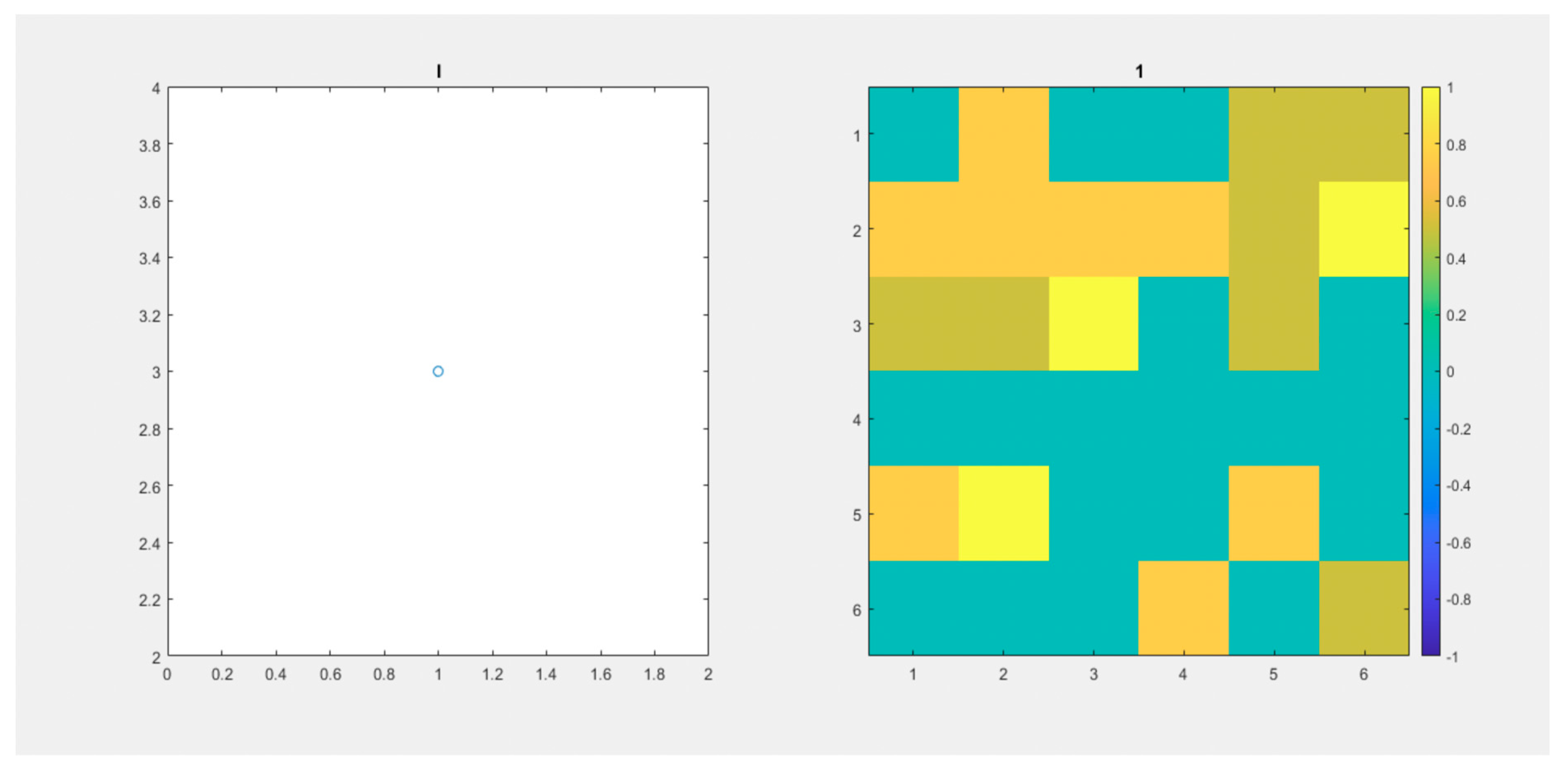
Figure 6.
(Video S3). 100x100 Lattice. and 200 days. On the left, we observe the number of infected individuals through time. On the right, the lattice.
Figure 6.
(Video S3). 100x100 Lattice. and 200 days. On the left, we observe the number of infected individuals through time. On the right, the lattice.
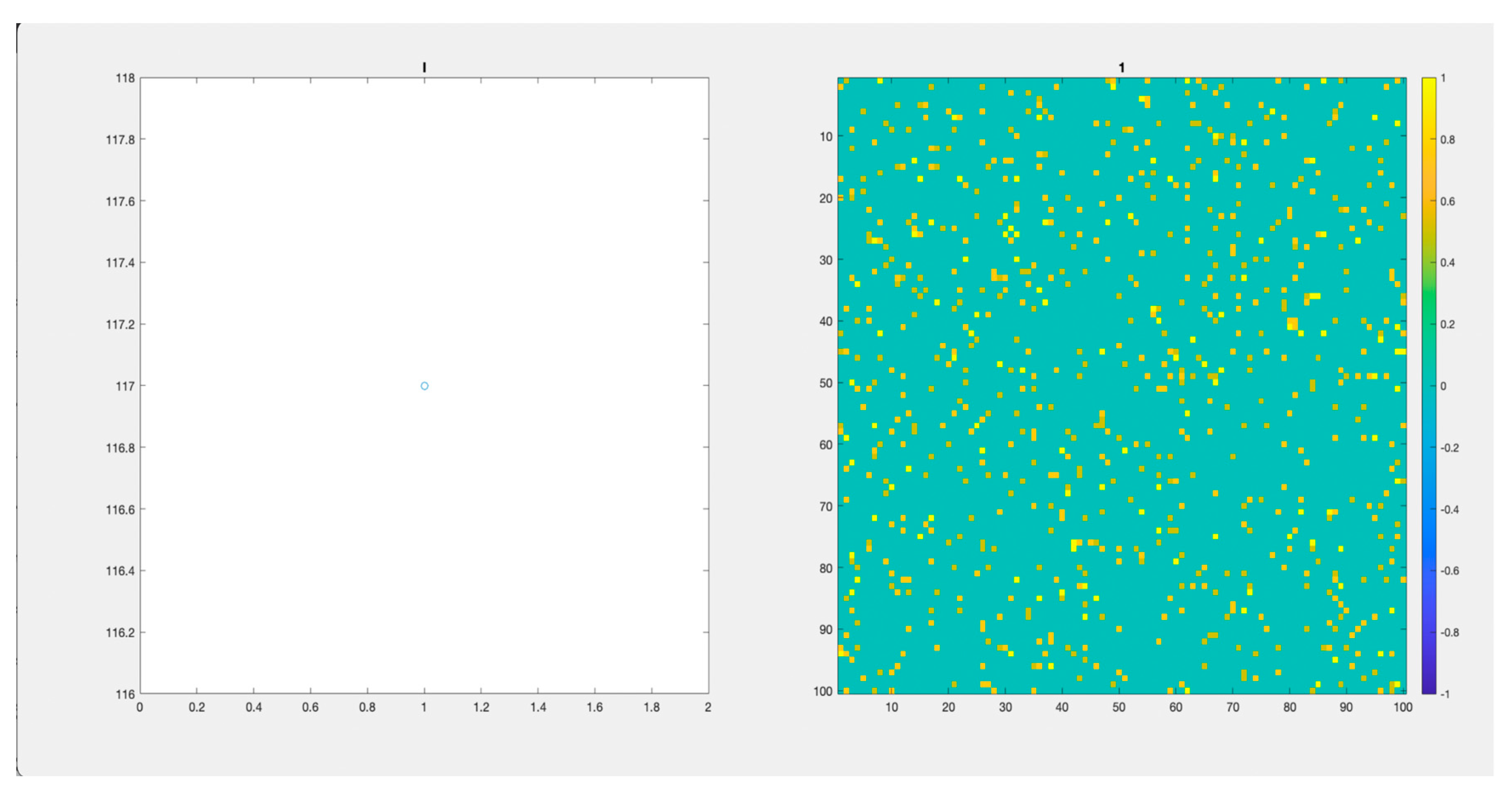
Figure 7.
(Video S4). 100x100 Lattice. and 200 days. Another initial distribution through the lattice. On the left, we observe the number of infected individuals through time. On the right the lattice.
Figure 7.
(Video S4). 100x100 Lattice. and 200 days. Another initial distribution through the lattice. On the left, we observe the number of infected individuals through time. On the right the lattice.
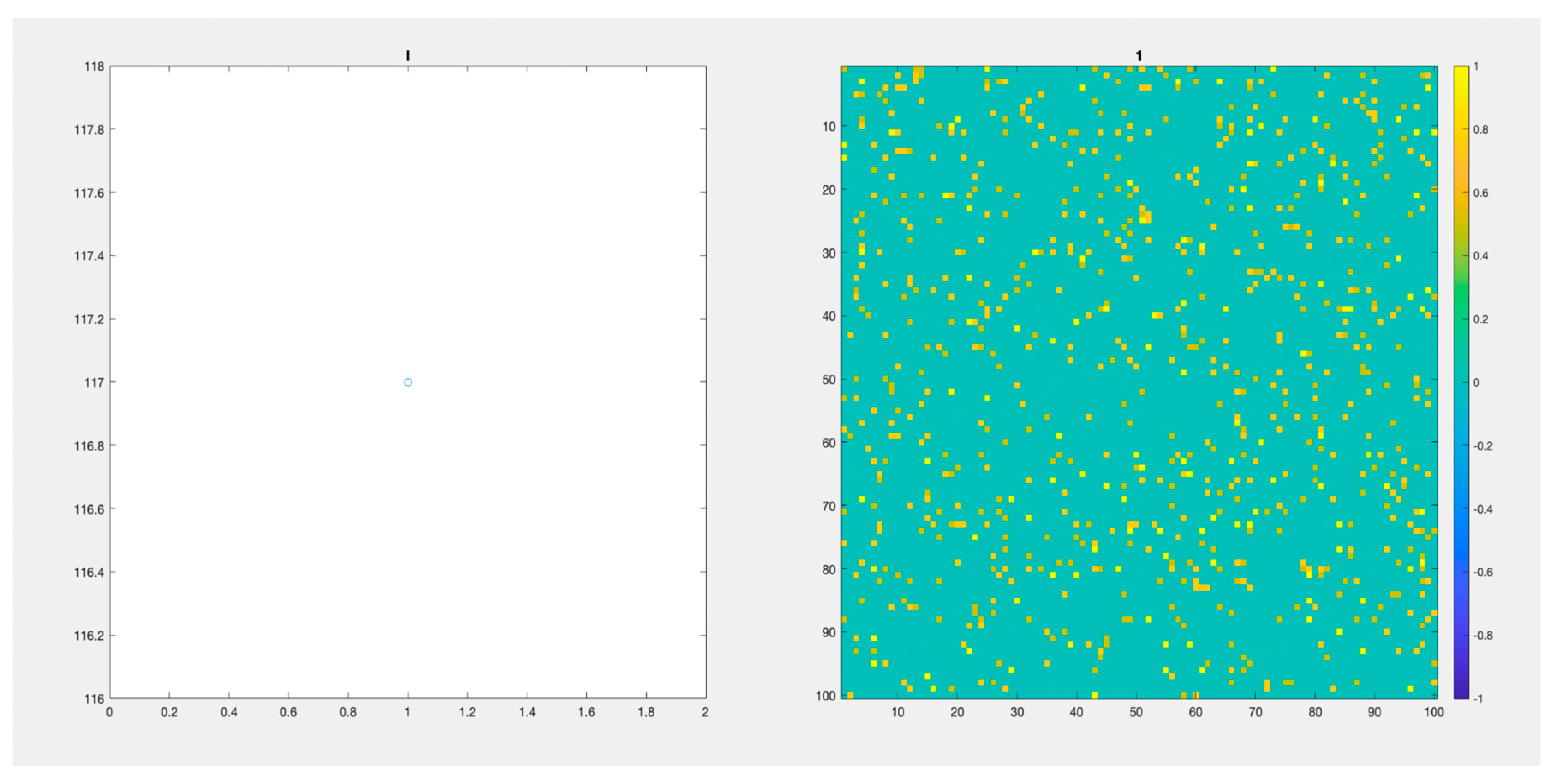
Figure 8.
100 different scenarios of 117 Infected individuals “seeded” into a population of 10,000 individuals. The period is (for all scenarios) 200 days.
Figure 8.
100 different scenarios of 117 Infected individuals “seeded” into a population of 10,000 individuals. The period is (for all scenarios) 200 days.
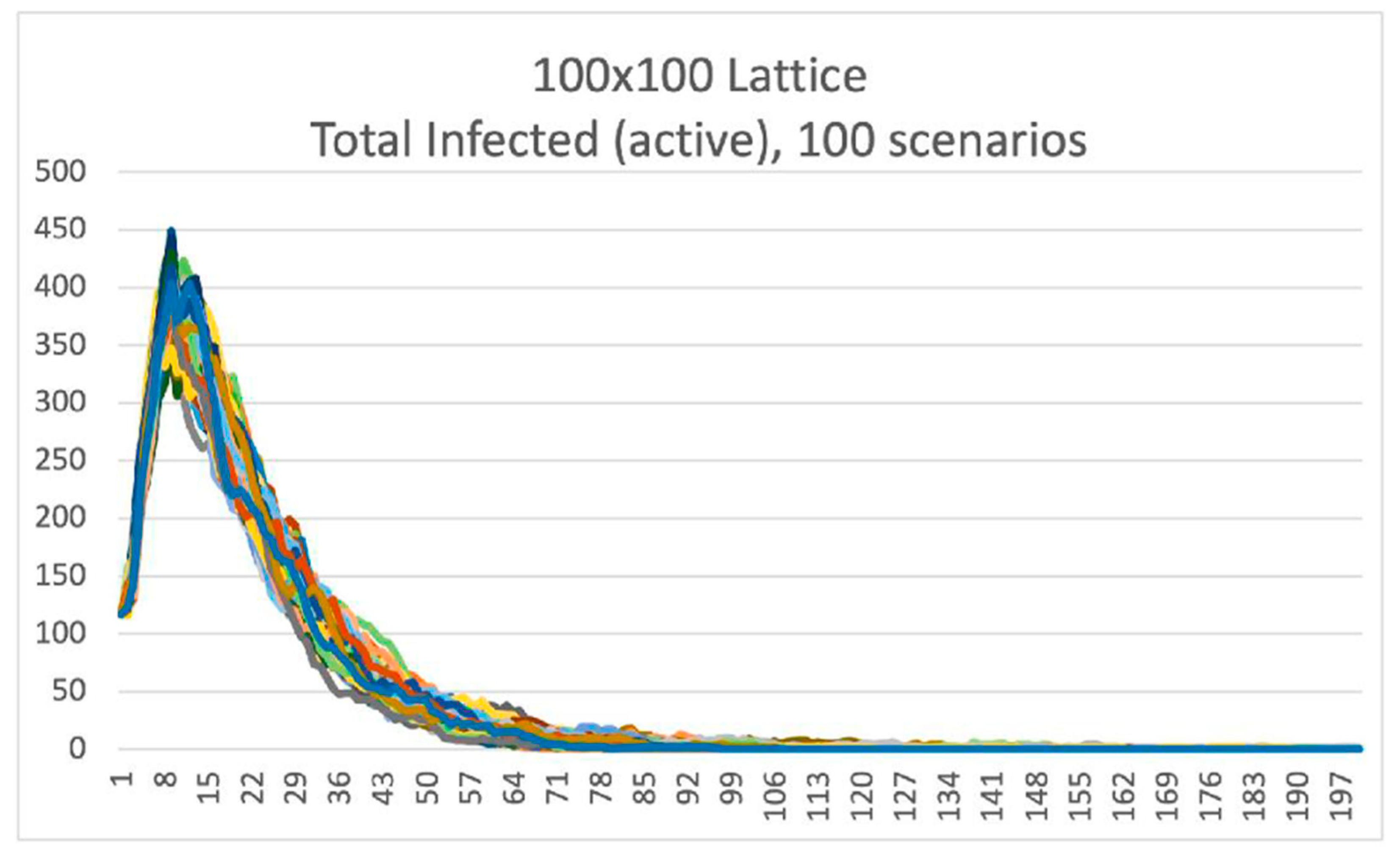
Figure 9.
The distribution of the maximum number of Infected individuals. It varies between 341 and 449 but concentrates in around 400 Infected individuals at the same time.
Figure 9.
The distribution of the maximum number of Infected individuals. It varies between 341 and 449 but concentrates in around 400 Infected individuals at the same time.
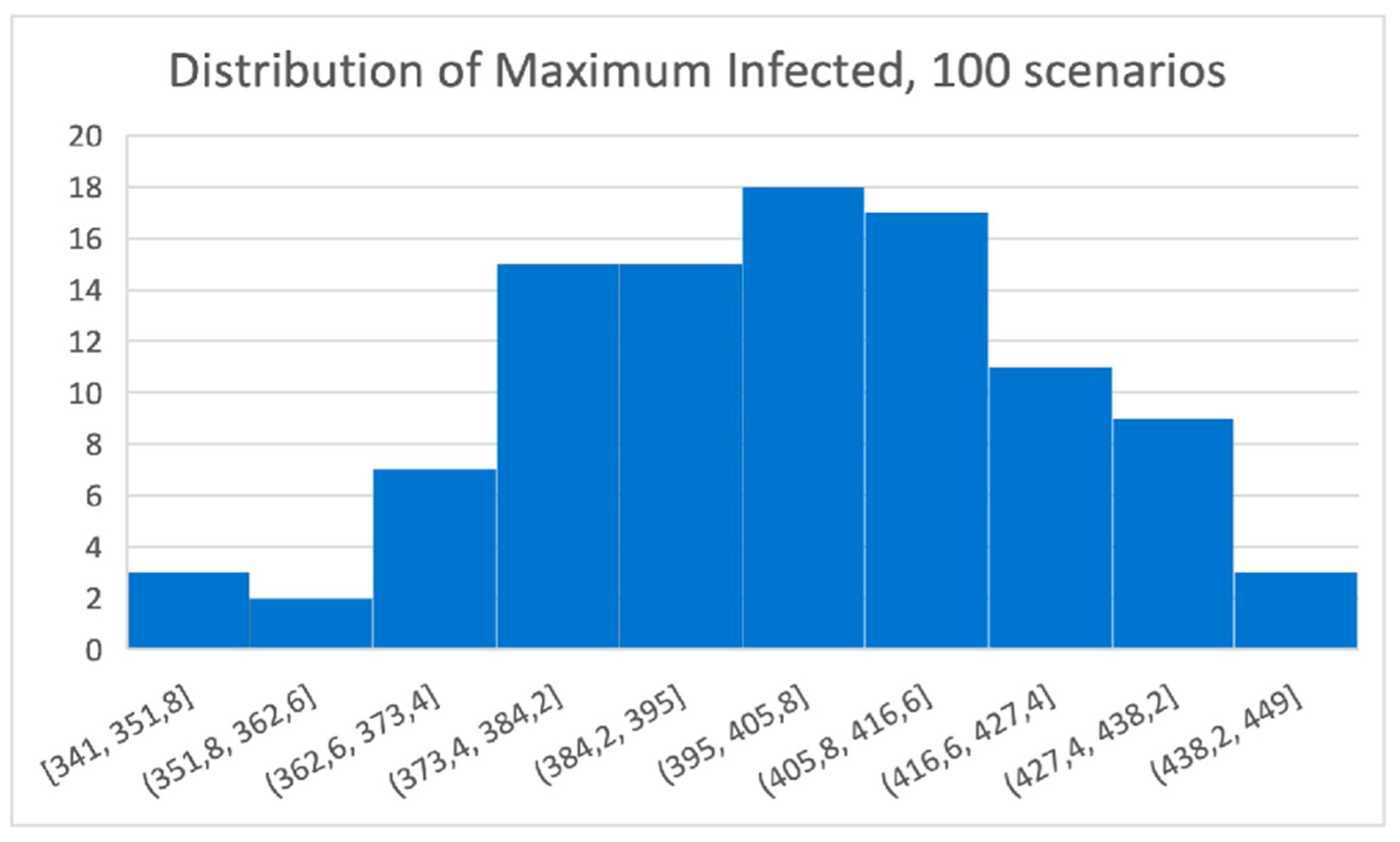
Figure 10.
(Video S5). 3282x3282 Lattice. and 1.000 days. On the left, we observe the number of Infected individuals through time. On the right, the lattice represents a population similar to Greece.
Figure 10.
(Video S5). 3282x3282 Lattice. and 1.000 days. On the left, we observe the number of Infected individuals through time. On the right, the lattice represents a population similar to Greece.
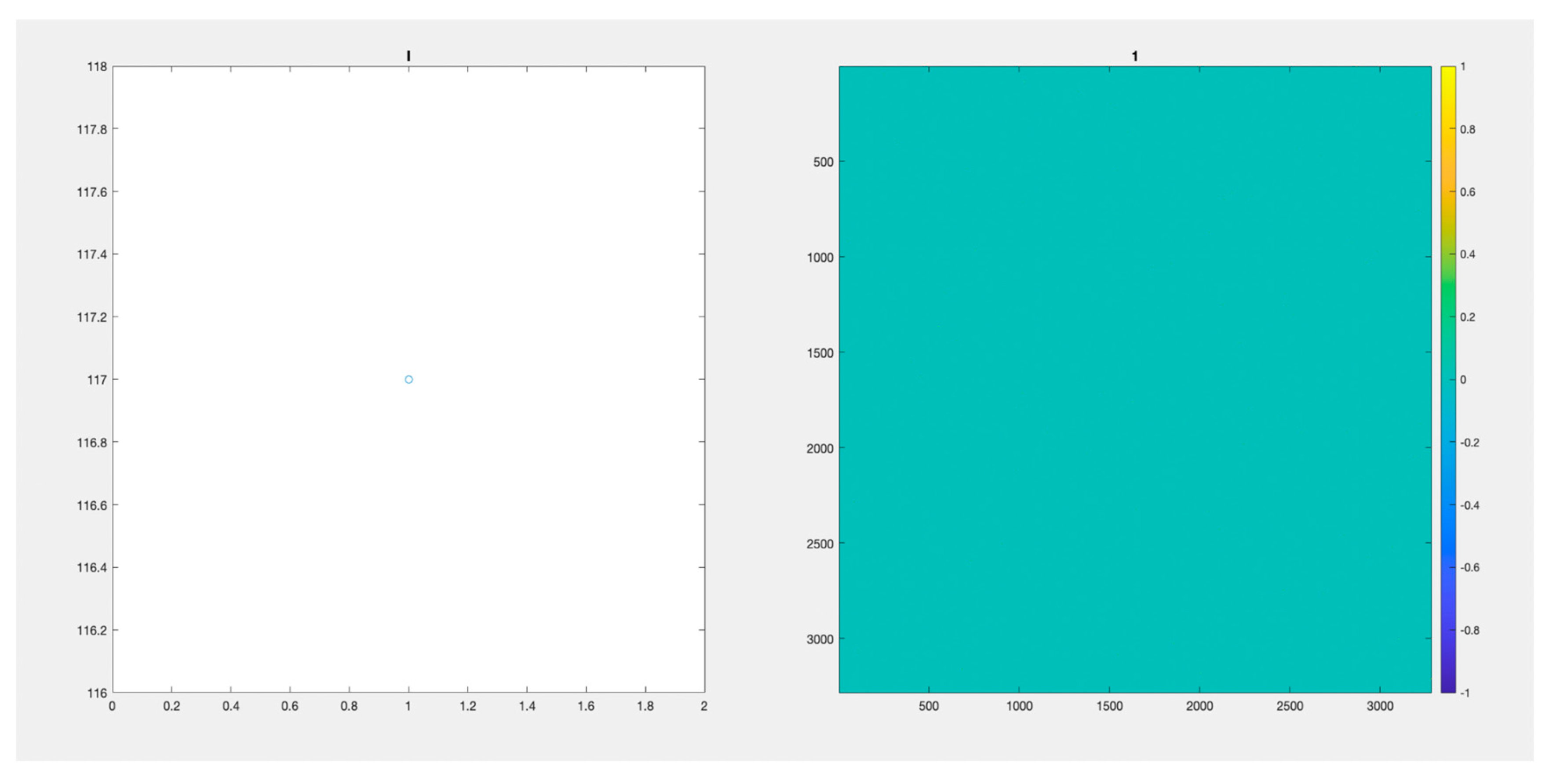

Table 1.
Parameters and Initial Conditions (for Exposed, E0, for Asymptomatic, A0 and Infected, I0) used in our experimentation.
Table 1.
Parameters and Initial Conditions (for Exposed, E0, for Asymptomatic, A0 and Infected, I0) used in our experimentation.
| Parameter | Value used |
|---|---|
| Recovery time (in days) | 6 |
| Immunity duration (in days) | 90 |
| Transmission rate (per infected) | 0.31 |
| Transmission rate (per asymptomatic) | 0.21 |
| Latent period (E → A) (in days) | 3 |
| Incubation period (E →I) (in days) | 5 |
| 2.65 | |
| 2.84 |
Disclaimer/Publisher’s Note: The statements, opinions and data contained in all publications are solely those of the individual author(s) and contributor(s) and not of MDPI and/or the editor(s). MDPI and/or the editor(s) disclaim responsibility for any injury to people or property resulting from any ideas, methods, instructions, or products referred to in the content. |
© 2023 by the authors. Licensee MDPI, Basel, Switzerland. This article is an open access article distributed under the terms and conditions of the Creative Commons Attribution (CC BY) license (http://creativecommons.org/licenses/by/4.0/).
Copyright: This open access article is published under a Creative Commons CC BY 4.0 license, which permit the free download, distribution, and reuse, provided that the author and preprint are cited in any reuse.